Magnetic trapping of ultracold Rydberg atoms in low angular momentum states

Abstract

We theoretically investigate the quantum properties of $nS$, $nP$, and $nD$ Rydberg atoms in a magnetic Ioffe-Pritchard trap. In particular, it is demonstrated that the two-body character of Rydberg atoms significantly alters the trapping properties opposed to point-like particles with identical magnetic moment. Approximate analytical expressions describing the resulting Rydberg trapping potentials are derived and their validity is confirmed for experimentally relevant field strengths by comparisons to numerical solutions of the underlying Schrödinger equation. In addition to the electronic properties, the center of mass dynamics of trapped Rydberg atoms is studied. In particular, we analyze the influence of a short-time Rydberg excitation, as required by certain quantum-information protocols, on the center of mass dynamics of trapped ground state atoms. A corresponding heating rate is derived and the implications for the purity of the density matrix of an encoded qubit are investigated.

I Introduction

During the past decade, powerful cooling techniques enabled remarkable experiments with ultracold atomic gases revealing a plethora of intriguing phenomena. Among the many fascinating systems are Rydberg atoms possessing extraordinary properties Gallagher (1994). Because of the large displacement of the valence electron and the ionic core, they are highly polarizable and, therefore, experience a strong dipole-dipole interaction amongst each other. In ultracold gases, the latter has been shown theoretically Jaksch et al. (2000); Lukin et al. (2001) and experimentally Tong et al. (2004); Singer et al. (2004); Cubel Liebisch et al. (2005); Vogt et al. (2007); van Ditzhuijzen et al. (2008) to entail a blockade mechanism thereby effectuating a collective excitation process of Rydberg atoms Heidemann et al. (2007); Reetz-Lamour et al. (2008); Johnson et al. (2008). Moreover, two recent experiments demonstrated the blockade between two single atoms a few $\mu$m apart Urban et al. (2009); Gaëtan et al. (2009). The dipole-dipole interaction renders Rydberg atoms also promising candidates for the implementation of protocols realizing two-qubit quantum gates Jaksch et al. (2000); Lukin et al. (2001). A prerequisite for the latter is, however, the availability of suitable environments enabling the controlled manipulation of single Rydberg atoms and preventing the dephasing of ground and Rydberg state.

Several works have focused on the issue of trapping Rydberg atoms based on electric Hyafil et al. (2004); Hogan and Merkt (2008), optical Dutta et al. (2000), or strong magnetic fields Choi et al. (2005a, b). Being omnipresent in experiments dealing with ultracold atoms, inhomogeneous magnetic fields seem predestined for trapping Rydberg atoms (even a two-dimensional permanent magnetic lattice of Ioffe-Pritchard microtraps for ultracold atoms has been realized experimentally Gerritsma et al. (2007); Whitlock et al. (2009)). Similar to ground state atoms, the magnetic trapping of Rydberg atoms originates from the interaction of its magnetic moment with the magnetic field. In particular, this allows utilizing trap geometries which are well-known from ground state atoms. In this spirit, theoretical studies recently demonstrated that Rydberg atoms can be tightly confined in a magnetic Ioffe-Pritchard (IP) trap Hezel et al. (2006, 2007) and that one-dimensional Rydberg gases can be created and stabilized by means of an additional electric field Mayle et al. (2007). However, the trapping mechanism relies in these studies on high angular momentum electronic states that have not been realized yet in experiments with ultracold atoms. In a very recent work, the authors expanded the former studies to low angular momentum $nS_{1/2}$ states and showed that the composite nature of Rydberg atoms, i.e., the fact that they consist of an outer electron far away from a compact ionic core, significantly alters their trapping properties opposed to point-like particles with the same magnetic moment Mayle et al. (2009). Furthermore, it has been demonstrated how the specific features of the Rydberg trapping potential can be probed by means of ground state atoms that are off-resonantly coupled to the Rydberg state via a two photon laser transition. In the present work, we provide a detailed derivation and discussion of the Rydberg energy surfaces presented in Ref. Mayle et al. (2009). Moreover, the trapping potentials arising for the $nS$, $nP$, and $nD$ states of ⁸⁷Rb are explored. As we are going to show, they possess a reduced azimuthal symmetry and a finite trap depth, which can be a few vibrational quanta only or less. Choosing the magnetic field parameters appropriately, on the other hand, trapping can be achieved with trap depths in the micro-Kelvin regime. Implications for quantum information protocols involving magnetically trapped Rydberg atoms are discussed.

In detail we proceed as follows. Section II contains a derivation of our working Hamiltonian for low angular momentum Rydberg atoms in a Ioffe-Pritchard trap which is solved by means of a hybrid computational approach employing basis-set and discretization techniques. Section III then introduces reasonable approximations which allow us to gain analytical solutions for the stationary Schrödinger equation and hence for the trapping potentials. In Sec. IV we analyze the resulting energy surfaces which serve as a potential for the center of mass motion of the Rydberg atom. The range of validity of our analytical approach is discussed. Section V is dedicated to the c.m. dynamics within the adiabatic potential surfaces. The question of how the c.m. state of a ground state atom is altered due to its short-time excitation to a Rydberg state is illuminated in Sec. VI. A heating rate associated with this process is derived. In Sec. VII, the effect of the same process on the purity of the density matrix of a qubit which is encoded in the hyperfine states of a ground state atom is discussed.

II Hamiltonian

Along the lines of Ref. Hezel et al. (2007) we model the mutual interaction of the highly excited valence electron and the remaining closed-shell ionic core of an alkali Rydberg atom by an effective potential which is assumed to depend only on the distance of the two particles. In our previous works Lesanovsky and Schmelcher (2005); Hezel et al. (2007, 2006); Mayle et al. (2007), this potential could be considered to be purely Coulombic since solely circular states with maximum electronic angular momentum were investigated. The low angular momentum states of alkali atoms, on the other hand, significantly differ from the hydrogenic ones because of the finite size and the electronic structure of the ionic core. However, the resulting core penetration, scattering, and polarization effects can be accounted for by employing a model potential of the form

$$V(r)\equiv V_{l}(r)=-\frac{Z_{l}(r)}{r}-\frac{\alpha_{c}}{2r^{4}}\big{[}1-e^{-(r/r_{c})^{6}}\big{]},$$ (1)

where $\alpha_{c}$ is the static dipole polarizability of the positive-ion core while the radial charge $Z_{l}(r)$ is given by

$$Z_{l}(r)=1+(z-1)e^{-a_{1}r}-r(a_{3}+a_{4}r)e^{-a_{2}r},$$ (2)

where $z$ is the nuclear charge of the neutral atom and $r_{c}$ is the cutoff radius introduced to truncate the unphysical short-range behavior of the polarization potential near the origin Marinescu et al. (1994). Note that $V_{l}(r)$ depends on the orbital angular momentum $l$ via its parameters, i.e., $a_{i}\equiv a_{i}(l)$ and $r_{c}\equiv r_{c}(l)$. The resulting binding energies are related to the effective quantum number $n^{*}$ and the quantum defect $\delta$ by $W=-\frac{1}{2{n^{*}}^{2}}=-\frac{1}{2(n-\delta)^{2}}$ Gallagher (1994); unless stated otherwise, all quantities are given in atomic units.

The coupling of the charged particles to the external magnetic field is introduced via the minimal coupling, $\mathbf{p}_{i}\rightarrow\mathbf{p}_{i}-q_{i}\mathbf{A}(\mathbf{r}_{i})$, with $i\in\{e,c\}$ denoting the valence electron and the remaining ionic core of a Rydberg atom, respectively; $q_{i}$ is the charge of the $i$-th particle and $\mathbf{A(x)}$ is the vector potential belonging to the magnetic field $\mathbf{B(x)}$. Including the coupling of the magnetic moments to the external field ($\bm{\mu}_{e}$ and $\bm{\mu}_{c}$ originate from the electronic and nuclear spins, respectively), our initial Hamiltonian in the laboratory frame reads (employing $q_{e}=-1$, $q_{c}=1$)

$$H={} \frac{1}{2}[\mathbf{p}_{e}+\mathbf{A}(\mathbf{r}_{e})]^{2}+\frac{1}{2M}[\mathbf{p}_{c}-\mathbf{A}(\mathbf{r}_{c})]^{2}$$

$$-\bm{\mu}_{e}\cdot\mathbf{B}(\mathbf{r}_{e})-\bm{\mu}_{c}\cdot\mathbf{B}(\mathbf{r}_{c})+V_{l}(r)+V_{so}(\mathbf{L}_{r},\mathbf{S})$$ (3)

with $r=|\mathbf{r}_{e}-\mathbf{r}_{c}|$ and $M$ being the mass of the ionic core. In contrast to our previous studies Lesanovsky and Schmelcher (2005); Hezel et al. (2006, 2007); Mayle et al. (2007), one has to take into account the fine structure of the atomic energy levels: For the magnetic field strengths investigated in this work, the spin-orbit interaction will lead to splittings larger than any Zeeman splitting encountered; it is given by

$$V_{so}(\mathbf{L}_{r},\mathbf{S})=\frac{\alpha^{2}}{2}\big{[}1-\frac{\alpha^{2}}{2}V_{l}(r)\big{]}^{-2}\frac{1}{r}\frac{\mathrm{d}V_{l}(r)}{\mathrm{d}r}\mathbf{L}_{r}\cdot\mathbf{S}$$ (4)

where $\mathbf{L}_{r}$ and $\mathbf{S}$ denote the angular momentum and spin of the valence electron, respectively. The term $[1-\alpha^{2}V_{l}(r)/2]^{-2}$ has been introduced to regularize the nonphysical divergence near the origin Condon and Shortley (1935). As usual, the field-free electronic eigenstates are labeled by the total electronic angular momentum $\mathbf{J=L}_{r}+\mathbf{S}$. We remark that the model potential $V_{l}(r)$ has been developed ignoring the fine structure; let us therefore briefly comment on the accuracy of Eq. (4) in reproducing the fine structure intervals. For the $40P$ state of rubidium, our approach yields a good quantitative agreement with the experimentally determined fine structure splitting, showing a deviation of less than one percent. This accuracy decreases for higher angular momenta; for the $40D$ state nevertheless a qualitative agreement is found.

The magnetic field configuration of the Ioffe-Pritchard trap is given by a two-dimensional quadrupole field in the $x_{1},x_{2}$-plane together with a perpendicular offset (Ioffe-) field in the $x_{3}$-direction. It can be created by several means. The “traditional” macroscopic realization uses four parallel current carrying Ioffe bars which generate the two-dimensional quadrupole field. Encompassing Helmholtz coils create the additional constant field Pritchard (1983). More recent implementations are for example the quic Esslinger et al. (1998) and the clover-leaf configuration Mewes et al. (1996). On a microscopic scale, the Ioffe-Pritchard trap has been implemented on atom chips by a Z-shaped wire Fortagh and Zimmermann (2007). The IP configuration can be parametrized as $\mathbf{B}(\mathbf{x})=\mathbf{B}_{c}+\mathbf{B}_{l}(\mathbf{x})$ with $\mathbf{B}_{c}=B\mathbf{e}_{3}$ and $\mathbf{B}_{l}(\mathbf{x})=G\left[x_{1}\mathbf{e}_{1}-x_{2}\mathbf{e}_{2}\right]$. The corresponding vector potential reads $\mathbf{A}(\mathbf{x})=\mathbf{A}_{c}(\mathbf{x})+\mathbf{A}_{l}(\mathbf{x})$ with $\mathbf{A}_{c}(\mathbf{x})=\frac{B}{2}\left[x_{1}\mathbf{e}_{2}-x_{2}\mathbf{e}_{1}\right]$ and $\mathbf{A}_{l}(\mathbf{x})=Gx_{1}x_{2}\mathbf{e}_{3}$, where $B$ and $G$ are the Ioffe field strength and the gradient, respectively. The quadratic term $\mathbf{B}_{q}\propto(x_{3}^{2}-\rho^{2}/2)\mathbf{e}_{3}$ that usually arises for a IP configuration can be exactly zeroed by geometry, which we are considering in the following. In actual experimental setups, $\mathbf{B}_{q}$ provides a weak confinement also in the $x_{3}$-direction. Omitting $\mathbf{B}_{q}$, the magnitude of the magnetic field at a certain position $\mathbf{x}$ in space is given by $|\mathbf{B}(\mathbf{x})|=\sqrt{B^{2}+G^{2}\rho^{2}}$, which yields a linear asymptote $|\mathbf{B}(\mathbf{x})|\rightarrow G\rho$ for large coordinates ($\rho=\sqrt{x_{1}^{2}+x_{2}^{2}}\gg B/G$) and a harmonic behavior $|\mathbf{B}(\mathbf{x})|\approx B+\frac{1}{2}G^{2}\rho^{2}$ close to the origin ($\rho\ll B/G$).

After introducing relative and c.m. coordinates ($\mathbf{r}$ and $\mathbf{R}$) and employing the unitary transformation $U=\exp\left[-\frac{i}{2}(\mathbf{B}_{c}\times\mathbf{r})\cdot\mathbf{R}\right]$, the Hamiltonian describing the Rydberg atom becomes

$$UHU^{\dagger}={} H_{A}+\frac{\mathbf{P}^{2}}{2M}+\tfrac{1}{2}[\mathbf{L}_{r}+2\mathbf{S}]\cdot\mathbf{B}_{c}-\bm{\mu}_{e}\cdot\mathbf{B}_{l}(\mathbf{R+r})$$

$$-\bm{\mu}_{c}\cdot\mathbf{B}(\mathbf{R})+\mathbf{A}_{l}(\mathbf{R+r})\cdot\mathbf{p}+\tfrac{1}{2}\mathbf{A}_{c}(\mathbf{r})^{2}+H_{\mathrm{corr}}\,.$$ (5)

Here, $H_{A}=\mathbf{p}^{2}/2+V_{l}(r)+V_{so}(\mathbf{L}_{r},\mathbf{S})$ is the Hamiltonian of an alkali atom possessing the energies $E_{nlj}^{el}=-\frac{1}{2}(n-\delta_{nlj})^{-2}$. $H_{\mathrm{corr}}=\frac{1}{2}\mathbf{A}_{l}(\mathbf{R+r})^{2}+\frac{1}{M}\mathbf{B}_{c}\cdot(\mathbf{r\times P})+U[V_{l}(r)+V_{so}(\mathbf{L}_{r},\mathbf{S})]U^{\dagger}-[V_{l}(r)+V_{so}(\mathbf{L}_{r},\mathbf{S})]$ are small corrections which can be neglected because of the following reasons: In the parameter regime we are focusing on, the diamagnetic contribution of the gradient field, $\mathbf{A}_{l}(\mathbf{R+r})^{2}$, is small compared to the one of the constant Ioffe field, $\mathbf{A}_{c}(\mathbf{r})^{2}$. The second contribution of $H_{\text{corr}}$ is negligible within our adiabatic approach since $\langle\mathbf{P}/M\rangle$ becomes negligible for ultracold temperatures compared to the relative motion $\langle\mathbf{p}/m\rangle$. Finally, the remaining terms couple to remote electronic states only and are therefore irrelevant.

The magnetic moments of the particles are connected to the electronic spin $\mathbf{S}$ and the nuclear spin $\mathbf{\Sigma}$ according to $\mbox{\boldmath$\mu$}_{e}=-\mathbf{S}$ and $\mbox{\boldmath$\mu$}_{c}=-\frac{g_{N}}{2M_{c}}\mathbf{\Sigma}$, with $g_{N}$ being the nuclear $g$-factor; because of the large nuclear mass, the term involving $\mbox{\boldmath$\mu$}_{c}$ is neglected in the following. We remark that the $Z$-component of the c.m. momentum commutes with the Hamiltonian (II); hence the longitudinal motion can be integrated out by employing plane waves $|K_{Z}\rangle=\exp(-iK_{Z}Z)$. In order to solve the remaining coupled Schrödinger equation, we employ a Born-Oppenheimer separation of the c.m. motion and the electronic degrees of freedom by projecting Eq. (II) on the electronic eigenfunctions $\psi_{\kappa}(\mathbf{r};\mathbf{R})$ that parametrically depend on the c.m. coordinates. We are thereby led to a set of decoupled differential equations governing the adiabatic c.m. motion within the individual two-dimensional energy surfaces $E_{\kappa}(\mathbf{R})$, i.e., the surfaces $E_{\kappa}(\mathbf{R})$ serve as potentials for the c.m. motion of the atom. The non-adiabatic (off-diagonal) coupling terms $\Delta T$ that arise within this procedure in the kinetic energy term can be neglected in our parameter regime since they are suppressed by the splitting between adjacent energy surfaces Hezel et al. (2006). As will be shown in Sec. III, the latter is proportional to the Ioffe field strength $B$, i.e., the non-adiabatic couplings are proportional to powers of $1/B$.

The electronic eigenfunctions and energies are found by a standard basis set method utilizing the field-free eigenfunctions $|\kappa\rangle=|njm_{j}ls\rangle$ of $H_{A}$ whose spin and angular parts $|jm_{j}ls\rangle$ are given by the spin-orbit coupled generalized spherical harmonics $\mathcal{Y}_{j,m_{j},l}$ Friedrich (1998). For the radial degree of freedom, a discrete variable representation (DVR) based on generalized Laguerre polynomials is employed McCurdy et al. (2003). The latter provides a non-uniform grid for the radial coordinate which is more dense close to the origin and hence especially suited for representing radial Rydberg wave functions. Since in the DVR scheme the potential matrix element evaluation is equivalent to a Gaussian quadrature rule, representing the Hamiltonian (II) – especially $V_{l}(r)$ and the derivative terms arising from the momentum operator $\mathbf{p}$ – becomes particularly efficient. The numerical diagonalization of the resulting Hamiltonian matrix (in the limit $\mathbf{P}\rightarrow 0$) then yields the electronic eigenfunctions $\psi_{\kappa}(\mathbf{r};\mathbf{R})$ and energies $E_{\kappa}(\mathbf{R})$ which both parametrically depend on the c.m. coordinates $\mathbf{R}$. Convergence is ensured by appropriately choosing the size of the field-free basis as well as the underlying DVR grid size.

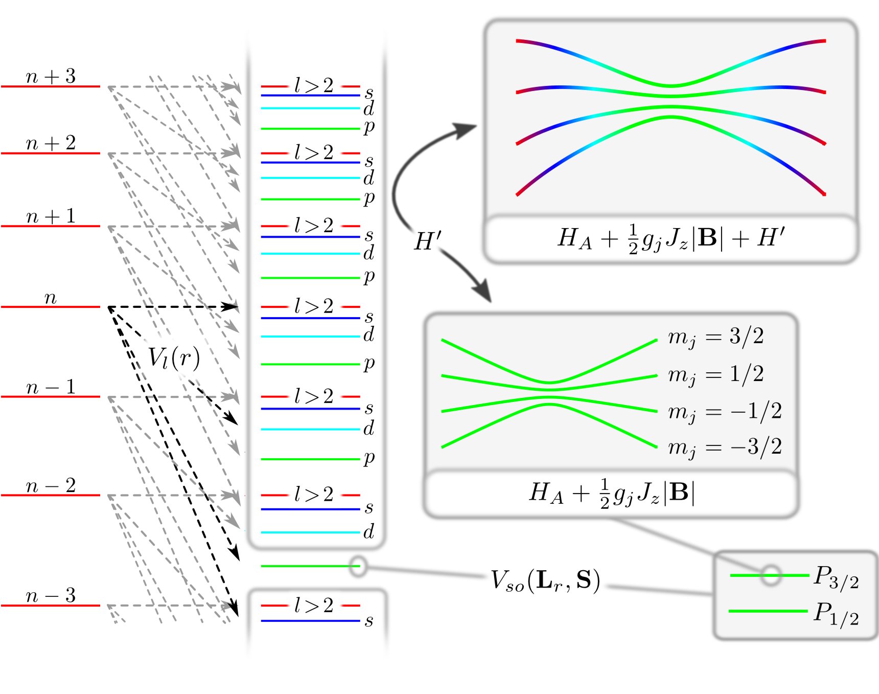
Figure 1: (Color online) Schematic overview of the energy scales and coupling terms involved. Starting from the degenerate hydrogen energy spectrum on the left, it is shown how the quantum defect – modeled by the potential $V_{l}(r)$ – separates the low angular momentum states. The spin-orbit coupling $V_{so}(\mathbf{L}_{r},\mathbf{S})$ then yields the fine structure splitting for fixed $l$. Within a given $j$-manifold, the Hamiltonian $H_{A}+\frac{1}{2}g_{j}m_{j}|\mathbf{B}|$ resembles the coupling of a point-like particle to the magnetic field $\mathbf{B}(\mathbf{R})$. The two-body character of the Rydberg atom, which is represented by $H^{\prime}$, only contributes if energetically remote levels are considered as well: it admixes states of different $n$, $l$, $j$, and $m_{j}$ thereby qualitatively changing the shape of the surfaces.

III Analytical Approach

While the above described numerical treatment of the electronic Hamiltonian offers accurate results, we derive in this section analytical but approximative expressions for the adiabatic energy surfaces, which provides us with a profound understanding of the underlying physics. We start by considering only a single fine structure manifold, i.e., fixed total angular momentum $j$ for given $l$. Such an assumption is motivated by the fact that the fine structure dominates over the Zeeman splitting for the field strengths we are interested in, cf. Fig. 1. Within this regime, the contribution $\mathbf{A}_{l}(\mathbf{R+r})\cdot\mathbf{p}=G(XY+Xy+xY+xy)p_{z}$ of Hamiltonian (II) can be simplified as follows. We rewrite

$$yp_{z}=\frac{1}{2}(yp_{z}-zp_{y})-\frac{i}{2}[yz,H_{A}]+\frac{i}{2}[yz,V_{l}(r)+V_{so}(\mathbf{L}_{r},\mathbf{S})]$$ (6)

bearing in mind that only the action of any involved operator within a single $j$-manifold is considered. The first commutator in the above equation then vanishes due to the degeneracy of the eigenenergies of $H_{A}$ and since no coupling to different $n$-, $l$-, or $j$-states is considered. Likewise, the second commutator in Eq. (6) vanishes since neither $V_{l}(r)$ nor $V_{so}(\mathbf{L}_{r},\mathbf{S})$ depend on the magnetic quantum number $m_{j}$. Hence, within a given $j$-manifold, the electronic part of Hamiltonian (II) can be approximated by

$$H_{e}=H_{A}+\frac{1}{2}\left[\mathbf{L}_{r}+2\mathbf{S}\right]\cdot\mathbf{B}(\mathbf{R})+GXYp_{z}+H_{r}\,,$$ (7)

where we substituted $yp_{z}\rightarrow\frac{1}{2}L_{x}$ and similarly $xp_{z}\rightarrow-\frac{1}{2}L_{y}$. The contribution $H_{r}=\mathbf{A}_{l}(\mathbf{r})\cdot\mathbf{p}+\mathbf{B}_{l}(\mathbf{r})\cdot\mathbf{S}+\tfrac{1}{2}\mathbf{A}_{c}(\mathbf{r})^{2}$ only depends on the relative coordinate and – as we will show later – for a wide range of field strengths can approximately be regarded as a mere energy offset to the electronic energy surfaces; we will restrict ourselves to this regime and hence omit $H_{r}$ in the following.

Table 1: Coefficients of the linear fit of $C_{i}(n)=C_{i}^{(0)}+C_{i}^{(1)}n$ in the range $35\leq n\leq 45$ for the $nS$, $nP$, and $nD$ states of the ⁸⁷Rb atom. Note that negative magnetic quantum numbers $m_{j}$ yield the same results as their positive counterparts and are consequently omitted. The fitted $C_{i}$ are calculated using Eq. (21) with $n^{\prime}\in[n-10,n+10]$.

State	$C_{x}^{(0)}$	$C_{x}^{(1)}$	$C_{z}^{(0)}$	$C_{z}^{(1)}$
$S_{1/2},m_{j}=1/2$	-0.4813	-0.00027	-0.4813	-0.00027
$P_{1/2},m_{j}=1/2$	-0.4484	-0.00148	-0.4484	-0.00148
$P_{3/2},m_{j}=1/2$	-0.4541	-0.00152	-0.4316	-0.00164
$P_{3/2},m_{j}=3/2$	-0.4391	-0.00160	-0.4616	-0.00149
$D_{3/2},m_{j}=1/2$	-0.4570	-0.00069	-0.4326	-0.00011
$D_{3/2},m_{j}=3/2$	-0.4407	-0.00030	-0.4652	-0.00088
$D_{5/2},m_{j}=1/2$	-0.4570	-0.00073	-0.4287	-0.00006
$D_{5/2},m_{j}=3/2$	-0.4500	-0.00057	-0.4429	-0.00040
$D_{5/2},m_{j}=5/2$	-0.4358	-0.00023	-0.4712	-0.00107

The first two terms of Hamiltonian (7) can be diagonalized analytically by applying the spatially dependent transformation

$$U_{r}=e^{-i\gamma(L_{x}+S_{x})}e^{-i\beta(L_{y}+S_{y})}$$ (8)

that rotates the $z$-axis into the local magnetic field direction; $\gamma$ and $\beta$ denote the rotation angles:

$$\sin\gamma =\frac{-GY}{\sqrt{B^{2}+G^{2}(X^{2}+Y^{2})}}\,,$$ (9)

$$\sin\beta =\frac{-GX}{\sqrt{B^{2}+G^{2}X^{2}}}\,,$$ (10)

$$\cos\gamma =\frac{\sqrt{B^{2}+G^{2}X^{2}}}{\sqrt{B^{2}+G^{2}(X^{2}+Y^{2})}}\,,$$ (11)

$$\cos\beta =\frac{B}{\sqrt{B^{2}+G^{2}X^{2}}}\,.$$ (12)

The transformed Hamiltonian becomes

$$U_{r}H_{e}U_{r}^{\dagger}=H_{A}+\tfrac{1}{2}g_{j}J_{z}\sqrt{B^{2}+G^{2}(X^{2}+Y^{2})}\,,+H^{\prime}$$ (13)

with $g_{j}=\frac{3}{2}+\frac{s(s+1)-l(l+1)}{2j(j+1)}$, $U_{r}H_{A}U_{r}^{\dagger}=H_{A}$, and $H^{\prime}=GXYU_{r}p_{z}U_{r}^{\dagger}$. Like for ground state atoms, the second term of Eq. (13) represents the coupling of a point-like particle to the magnetic field via its magnetic moment $\bm{\mu}=\frac{1}{2}\mathbf{L}_{r}+\mathbf{S}$.

As depicted in Fig. 1, $H^{\prime}$ couples to different $n$, $l$, $j$, and $m_{j}$ and hence vanishes within one $j$-manifold. The first two terms of Eq. (13), on the other hand, are diagonal, giving rise to the electronic potential energy surface

$$E_{\kappa}^{(0)}(\mathbf{R})=E_{\kappa}^{el}+\tfrac{1}{2}g_{j}m_{j}\sqrt{B^{2}+G^{2}(X^{2}+Y^{2})}$$ (14)

for a given electronic state $|\kappa\rangle=|njm_{j}ls\rangle$. Note that such a state refers to the rotated frame of reference. Only there, $m_{j}$ constitutes a good quantum number; in the laboratory frame of reference $m_{j}$ is not conserved. The surfaces Eq. (14) are rotationally symmetric around the $Z$-axis and confining for $m_{j}>0$. For small radii ($\rho=\sqrt{X^{2}+Y^{2}}\ll B/G$) an expansion up to second order yields a harmonic potential

$$E_{\kappa}^{(0)}(\rho)\approx E_{\kappa}^{el}+\tfrac{1}{2}g_{j}m_{j}B+\frac{1}{2}M\omega^{2}\rho^{2}$$ (15)

with the trap frequency defined by $\omega=G\sqrt{\frac{g_{j}m_{j}}{2MB}}$ while we find a linear behavior $E_{\kappa}^{(0)}(\rho)\approx E_{\kappa}^{el}+\tfrac{1}{2}g_{j}m_{j}G\rho$ when the center of mass is far from the $Z$-axis ($\rho\gg B/G$). In the harmonic part of the potential, the c.m. energies are thus given by

$$E_{\kappa,\nu}^{cm}=E_{\kappa}^{(0)}(0)+(\nu+1)\omega\>,\;\nu=\nu_{x}+\nu_{y}\in\mathbb{N}$$ (16)

with a splitting of $\omega$ between adjacent c.m. states; see Sec. V for a more detailed discussion. The separation between adjacent electronic energy surfaces at the origin, on the other hand, is given by $\Delta E_{\kappa}=\tfrac{1}{2}g_{j}B$. The size of the c.m. ground state ($\nu=0$) in such a harmonic potential evaluates to $\langle\rho\rangle=\sqrt{\pi}/2\sqrt{M\omega}$ Hezel et al. (2007).

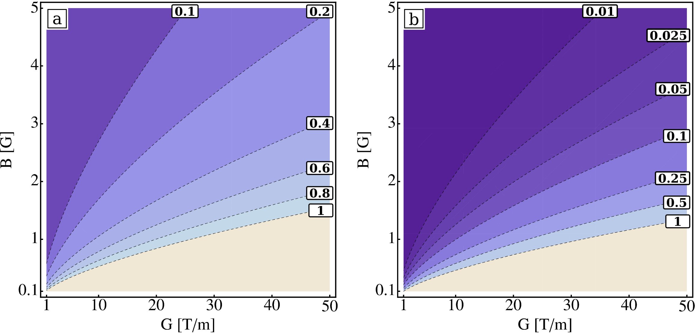
Figure 2: (Color online) Range of validity for deriving Eq. (24). (a) $2G^{2}X^{2}/B^{2}\ll 1$ resulting in $X\ll B/\sqrt{2}G$. In the figure, the value $X_{+}/(B/\sqrt{2}G)$ is shown which should be $\ll 1$. Figure (b) shows $G^{2}X_{0}^{2}/B^{2}$ which should be $\ll 1$ as well. In both cases $l=2,j=m_{j}=5/2$ is used.

The remaining term $H^{\prime}$ of Hamiltonian (13) can be treated perturbatively. While it vanishes in first order, second-order perturbation theory yields

$$E_{\kappa}^{(2)}(\mathbf{R}) =G^{2}X^{2}Y^{2}\sum_{\kappa^{\prime}\neq\kappa}\frac{\big{|}\langle\kappa|U_{r}p_{z}U_{r}^{\dagger}|\kappa^{\prime}\rangle\big{|}^{2}}{E_{\kappa}^{el}-E_{\kappa^{\prime}}^{el}}$$ (17)

$$\approx G^{2}X^{2}Y^{2}\sum_{\kappa^{\prime}\neq\kappa}(E_{\kappa}^{el}-E_{\kappa^{\prime}}^{el})\times\big{|}\langle\kappa|U_{r}zU_{r}^{\dagger}|\kappa^{\prime}\rangle\big{|}^{2}$$ (18)

where $\kappa=|njm_{j}ls\rangle$ are the eigenstates of the transformed Hamiltonian $U_{r}H_{e}U_{r}^{\dagger}-H^{\prime}$, cf. Eq. (13). Since $E_{\kappa}^{(0)}(\mathbf{R})$ resembles the confinement of a ground state atom, we attribute $E_{\kappa}^{(2)}(\mathbf{R})$ to the composite nature of the Rydberg atom, i.e., the fact that it consists of a Rydberg electron far apart from its ionic core. Like the magnetic field itself, $E_{\kappa}^{(2)}(\mathbf{R})$ shows no continuous azimuthal symmetry but rather a discrete one.

Equation (18) is derived by employing $U_{r}p_{z}U_{r}^{\dagger}=p_{x}\sin\beta-p_{y}\sin\gamma\cos\beta+p_{z}\cos\gamma\cos\beta$ and $\mathbf{p}=i[H_{A},\mathbf{r}]-i[V_{l}(r)+V_{so},\mathbf{r}]\approx i[H_{A},\mathbf{r}]$ . Expanding the modulus square in Eq. (18), one obtains mixed terms of the form $\langle\kappa|x|\kappa^{\prime}\rangle^{*}\langle\kappa|y|\kappa^{\prime}\rangle+\langle\kappa|x|\kappa^{\prime}\rangle\langle\kappa|y|\kappa^{\prime}\rangle^{*}$. Employing the standard basis of spherical harmonics and consequently using $\langle\kappa|x|\kappa^{\prime}\rangle\in\mathbb{R}$ as well as $\langle\kappa|y|\kappa^{\prime}\rangle=-\langle\kappa|y|\kappa^{\prime}\rangle^{*}$, this sum vanishes. The matrix element of $z$ obeys a different selection rule, namely, $\Delta m_{l}=0$ opposed to $\Delta m_{l}=\pm 1$ of $x$ and $y$; hence, mixed terms involving $\langle\kappa|z|\kappa^{\prime}\rangle$ vanish as well. Consequently, only the matrix elements $|\langle\kappa|x|\kappa^{\prime}\rangle|^{2}$, $|\langle\kappa|y|\kappa^{\prime}\rangle|^{2}$, and $|\langle\kappa|z|\kappa^{\prime}\rangle|^{2}$ remain and the second order energy contribution can be parametrized as

$$E_{\kappa}^{(2)}(\mathbf{R})={} G^{2}X^{2}Y^{2}\big{(}C_{x}\sin^{2}\!\beta$$

$$+C_{y}\sin^{2}\!\gamma\cos^{2}\!\beta+C_{z}\cos^{2}\!\gamma\cos^{2}\!\beta\big{)}$$ (19)

$$={} C_{z}G^{2}X^{2}Y^{2}$$

$$\times\Big{[}1+\frac{C_{x}-C_{z}}{C_{z}}\left(\sin^{2}\!\beta+\sin^{2}\!\gamma\cos^{2}\!\beta\right)\Big{]}.$$ (20)

with

$$C_{i}=\sum_{\kappa^{\prime}\neq\kappa}(E_{\kappa}^{el}-E_{\kappa^{\prime}}^{el})|\langle\kappa|x_{i}|\kappa^{\prime}\rangle|^{2}$$ (21)

where $C_{x}=C_{y}=C_{z}\equiv C$ for $l=0$ and $C_{x}=C_{y}$ otherwise (since $|\langle\kappa|x|\kappa^{\prime}\rangle|=|\langle\kappa|y|\kappa^{\prime}\rangle|$). Note that the parameters $C_{i}$ depend on the state $\kappa$ under investigation. Since $E_{\kappa}^{el}-E_{\kappa^{\prime}}^{el}\propto n^{-3}$ and $|\langle\kappa|x_{i}|\kappa^{\prime}\rangle|^{2}\propto n^{4}$, a linear scaling of $E_{\kappa}^{(2)}(\mathbf{R})$ with the quantum number $n$ is anticipated, i.e., $C_{i}(n)=C_{i}^{(0)}+C_{i}^{(1)}n$. Resulting from a fit of calculated $C_{i}$ values within the range $35\leq n\leq 45$, in Tab. 1 the coefficients $C_{i}^{(j)}$ are tabulated for the $nS$, $nP$, and $nD$ states of the ⁸⁷Rb atom. All considered states show a similar behavior: The magnitude of $C_{i}$ is close to $-1/2$ and shows a rather weak $n$-dependence. In particular, $C_{x}\approx C_{z}$ and therefore $E_{\kappa}^{(2)}(\mathbf{R})\approx C_{z}\cdot G^{2}X^{2}Y^{2}$, cf. Eq. (20). We remark that for smaller $n$, $C_{i}(n)$ deviates from the linear behavior in favor of a more rapid decrease.

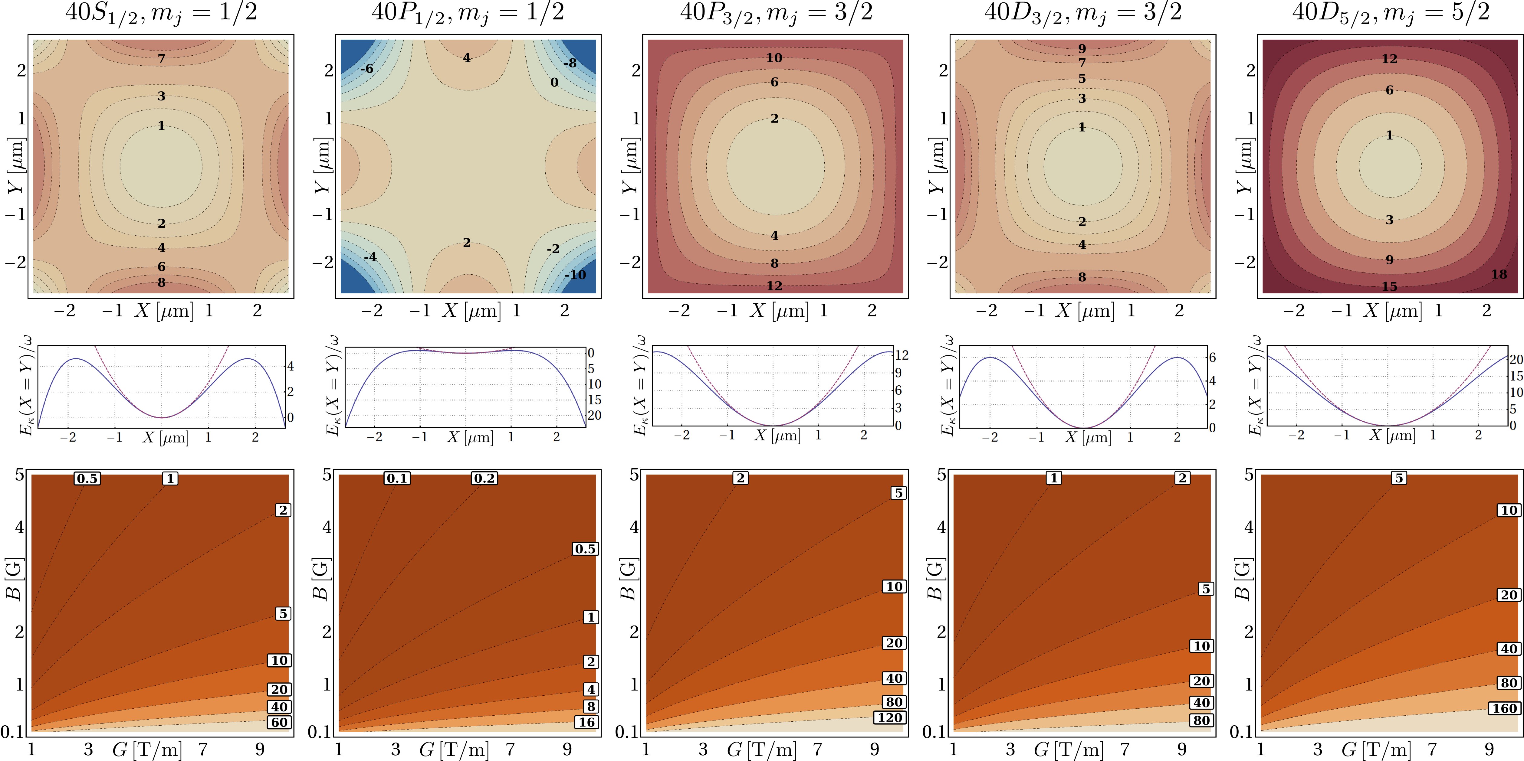
Figure 3: (Color online) First Row: Contour plots of the electronic potential energy surfaces $E_{\kappa}(\mathbf{R})$ of the $40S_{1/2}$ (first column), $40P_{1/2}$ (second column), $40P_{3/2}$ (third column), $40D_{3/2}$ (fourth column), and $40D_{5/2}$ (fifth column) states with $m_{j}=j$ for the magnetic field configuration $B=1$ G, $G=2.5$ T/m. Second Row: Section along $X=Y$ of the same energy surfaces; the contribution of $E_{\kappa}^{(0)}(\mathbf{R})$ (dashed lines) is shown in addition. Third Row: Depth of the potentials as given by Eq. (25) as a function of the magnetic field configuration. For all subfigures, the energy scale is given in terms of the trap frequency $\omega=G\sqrt{g_{j}m_{j}/2MB}$.

In the last part of this section, let us reconsider the adiabatic energy surfaces for the c.m. motion, including now the contribution of $H^{\prime}$. That is, we investigate the approximate, but analytical solutions

$$E_{\kappa}(\mathbf{R})\equiv E_{\kappa}^{(0)}(\mathbf{R})+E_{\kappa}^{(2)}(\mathbf{R})-E_{\kappa}^{el},$$ (22)

of Hamiltonian (7). In particular, we concentrate on the diagonal of the surfaces ($X=Y$) where $E_{\kappa}^{(2)}(\mathbf{R})$ is maximal. The approximation $C_{x}=C_{z}$ (which is exact for $nS_{1/2}$ states) then yields

$$E_{\kappa}(X=Y)=\frac{1}{2}g_{j}m_{j}\sqrt{B^{2}+2G^{2}X^{2}}+C_{z}G^{2}X^{4}\,,$$ (23)

which shows only a local minimum at the origin since the surface drops off for large c.m. coordinates when $E_{\kappa}^{(2)}(\mathbf{R})$ dominates (note that $C_{z}<0$), see also Fig. 3. The positions of the maxima which enclose the minimum are approximately given by

$$X_{\pm}\approx\pm\left(\frac{G^{2}}{B^{2}}-\frac{4BC_{z}}{g_{j}m_{j}}\right)^{-1/2}\approx\pm X_{0}\left(1-\frac{G^{2}}{2B^{2}}X_{0}^{2}\right)$$ (24)

with the length scale $X_{0}=\sqrt{\frac{g_{j}m_{j}}{4B|C_{z}|}}$ only depending on the Ioffe field strength. The depth of the potential well associated with the minimum correspondingly evaluates to

$$\Delta E_{\kappa}={} E_{\kappa}(X=Y=X_{+})-E_{\kappa}(0)$$ (25)

$$\approx{} \frac{1}{2}g_{j}m_{j}\frac{G^{2}X_{0}^{2}}{B}\left(1-\frac{G^{2}X_{0}^{2}}{B^{2}}\right)$$

$$+ C_{z}G^{2}X_{0}^{4}\left(1-2\frac{G^{2}X_{0}^{2}}{B^{2}}\right).$$ (26)

Note that the first approximation in Eq. (24) holds for $2G^{2}X^{2}/B^{2}\ll 1$ and the second one for $G^{2}X_{0}^{2}/B^{2}\ll 1$. The corresponding range of validity is illustrated in Fig. 2: For a Ioffe field strength of $B=1$ G, the above approximations hold for gradients up to $10$ T/m; at higher $B$ even larger gradients are eligible.

IV Trapping potentials

In the following section we are going to discuss the calculated electronic potential energy surfaces for the $nS$, $nP$, and $nD$ states of the ⁸⁷Rb atom in detail. In particular, the range of validity of the above derived analytic expression [Eq. (22)] is demonstrated. As a general example, we address the magnetic field configuration $B=1$ G, $G=2.5\,$Tm^-1, which yields a trap frequency of $\omega=2\pi\times 319$ Hz. A similar field configuration is also found in current experiments Loew et al. .

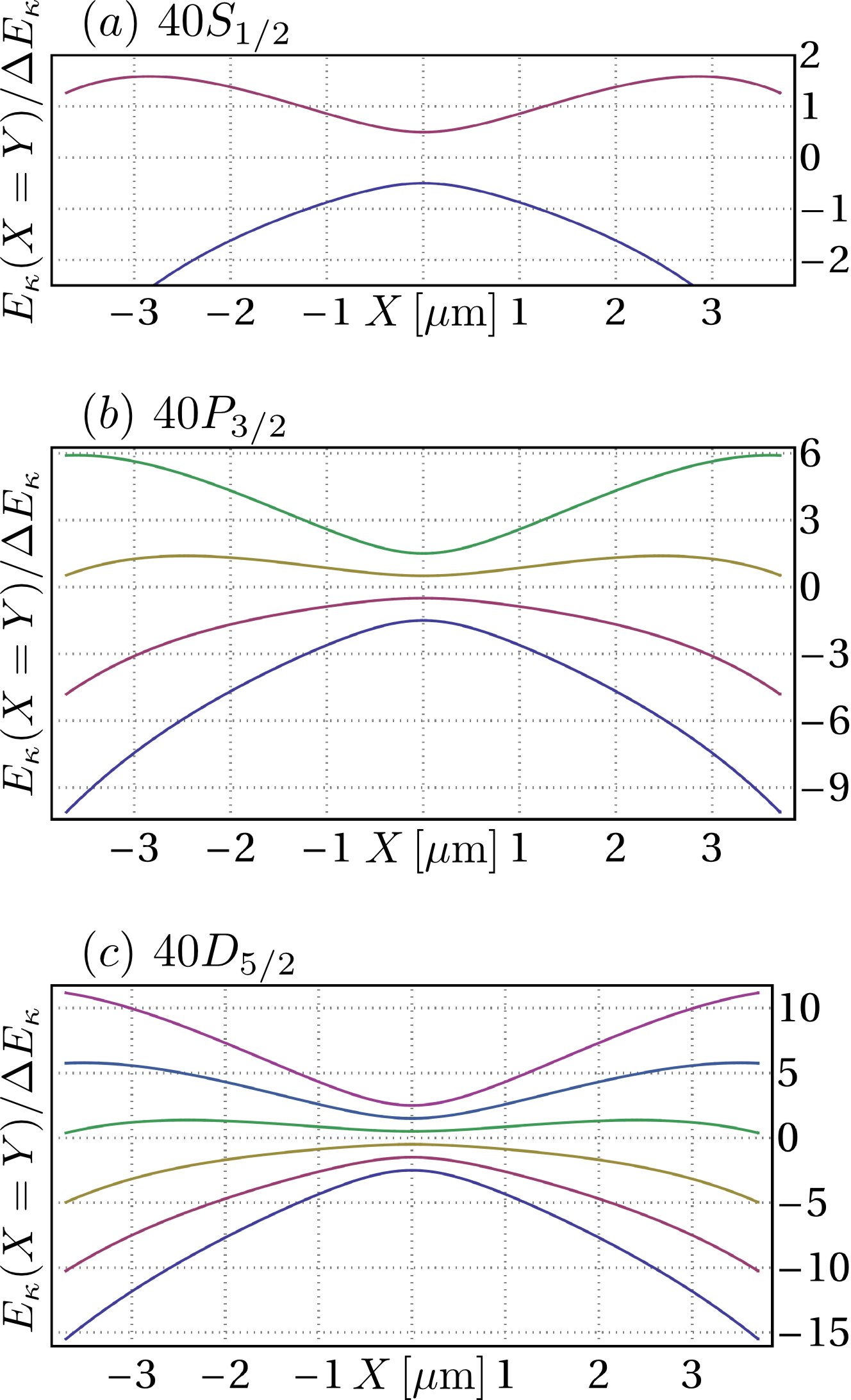
Figure 4: (Color online) Sections along $X=Y$ of the energy surfaces of the (a) $40S_{1/2}$, (b) $40P_{3/2}$, and (c) $40D_{5/2}$ states for the field configuration $B=0.1$ G, $G=10$ T/m, which yields a trap frequency of $\omega/\sqrt{g_{j}m_{j}}=2\pi\times 4$ kHz.

In Figure 3 the electronic potential energy surfaces $E_{\kappa}(\mathbf{R})$ of the $40S_{1/2}$, $40P_{1/2}$, $40P_{3/2}$, $40D_{3/2}$, and $40D_{5/2}$ states with $m_{j}=j$ are illustrated. In addition, also sections along $X=Y$ of these surfaces are provided. On a first glance, the energy surfaces originating from different electronic states seem to differ quite substantially. However, qualitatively they are very similar, as we are going to argue in the following. For all surfaces presented in Fig. 3, the contribution of the composite character of the Rydberg atom, i.e., $E_{\kappa}^{(2)}(\mathbf{R})$ changes the azimuthal symmetry of $E_{\kappa}^{(0)}(\mathbf{R})$ into a four-fold one. Moreover, the interplay between the harmonic confinement $E_{\kappa}^{(0)}(\mathbf{R})$ and the unbounded contribution $E_{\kappa}^{(2)}(\mathbf{R})$ gives rise to a finite trap depth along the diagonal $X=Y$; see second row of Fig. 3. Since the coefficient $C_{z}$ of $E_{\kappa}^{(2)}(\mathbf{R})$ is approximately of the same magnitude for all states considered, cf. Tab. 1, the trap depth depends on the magnitude of the magnetic moment $\bm{\mu}\propto g_{j}\mathbf{J}$. Consequently, the $j=m_{j}=l+1/2$ electronic states show a deeper confinement than their $j=m_{j}=l-1/2$ counterparts and the depth increases further with increasing orbital angular momentum $l$. For the examples given in Fig. 3 this means that the quadratic approximation to the trapping potential for the $40S_{1/2}$ state is already violated at about two oscillator energies, while for the $40D_{5/2}$ it is fine up to $10\,\omega$. This trend is confirmed in the third row of Fig. 3 where the depth of the potential as a function of the field configuration is displayed: For the $40D_{5/2}$ state, the trap depth easily exceeds $100\,\omega$ within the given parameter range, while in the case of the $40S_{1/2}$ state there is a substantial regime of field strengths where not a single center of mass state can be confined, i.e., the trap depth being $<1\,\omega$. Nevertheless, also for the $40S_{1/2}$ Rydberg state the field parameters $B$ and $G$ can be adjusted such that trapping is possible, i.e., the trap depth being much larger than the trap frequency. Similarly, the trapping potential of the $40D_{5/2}$ Rydberg state can be chosen very shallow by going to sufficiently strong Ioffe fields. We remark that the results presented in Fig. 3 are given in units of the trap frequency $\omega=G\sqrt{g_{j}m_{j}/2MB}$; the latter holds, of course, only near the origin. For larger radii, the contribution $E_{\kappa}^{(2)}(\mathbf{R})$ flattens the potential resulting in smaller trap frequencies and hence in a higher number of center of mass states that can be confined. Moreover, for very high gradients the harmonic expansion of the magnetic field strength becomes progressively worse.

As can be deduced from the third row of Fig. 3, increasing the relative strength of the field gradient, i.e., either increasing $G$ directly or decreasing the offset field $B$ for fixed $G$, leads to a larger number of bound center of mass states – independently of the state under consideration. However, since the anti-trapping contribution $E_{\kappa}^{(2)}(\mathbf{R})$ quadratically increases with the field gradient $G$, we expect this trend to reverse for sufficiently high gradients. Indeed, for a Ioffe field of $B=1\,$G the trap depth starts to decrease for field gradients $G\gtrsim 200\,\text{Tm}^{-1}$; for $B=0.1\,$G this trend already starts at $G\gtrsim 5\,\text{Tm}^{-1}$. Similarly, for a fixed field gradient together with a decreasing offset field $B$ we find a decrease of the trap depth if $B\lesssim 0.15\,$G or $B\lesssim 0.03\,$G for $G=10\,\text{Tm}^{-1}$ and $G=1\,\text{Tm}^{-1}$, respectively.

In the following, let us investigate the question if electronic energy surfaces belonging to different states intersect each other. In Refs. Hezel et al. (2007, 2006), where high angular momentum states are considered, this issue is essential: there, the high level of degeneracy of the system leads to non-adiabatic crossings of the surfaces. As a consequence, only the circular electronic state ($m_{l}=l=n-1$) provides stable trapping. For the low angular momentum states of ⁸⁷Rb we are considering here, however, the fine structure splitting for different $j$ and the varying quantum defect for different $l$ separate the energy surfaces by lifting the degeneracy, therefore preventing their crossing. As a result, it is sufficient in our case to investigate the energy surface spectrum for fixed $j$, i.e., only as a function of the magnetic quantum number. In Figure 4, sections along the diagonal of the energy surfaces of the multiplets of the $40S_{1/2}$, $40P_{3/2}$, and $40D_{5/2}$ states are presented. In order to show a strong spatial dependence, we choose an extreme case concerning the ratio of the Ioffe field compared to the gradient field, namely, $B=0.1$ G, $G=10$ T/m. Even for such a high gradient (of course much higher gradients can be achieved on atom chips), the energy surfaces remain well separated with a minimum distance of $\frac{1}{2}g_{j}B$ at the trap center. Hence, each surface can be considered separately for trapping and our adiabatic approach is not limited by non-adiabatic interactions. Note that the anti-trapping of $m_{j}<0$ states is even enhanced by the contribution $E_{\kappa}^{(2)}(\mathbf{R})$.

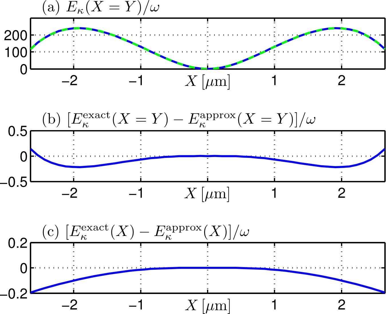
Figure 5: (Color online) (a) Section along $X=Y$ of the energy surface of the $40D_{5/2},m_{j}=5/2$ state for the field configuration $B=1$ G, $G=100$ T/m which yields a trap frequency of $\omega=2\pi\times 22.1$ kHz near the origin. The solid line is yield by the numerical diagonalization of Hamiltonian (II), the dashed one by Eq. (22). The surfaces have been offset to zero at the origin. (b) Difference (in terms of the trap frequency $\omega$) between the analytic expression Eq. (22) and the result of the numerical diagonalization of Hamiltonian (II). (c) Same as (b) but for $Y=0$ rather than $X=Y$.

The above investigations employ the analytical expression Eq. (22) rather than the exact numerical solutions of Hamiltonian (II). Hence an estimation of the range of validity of our results is necessary. To this end, we provide in Fig. 5(a) a comparison between the analytical expression according to Eq. (22) and the numerical diagonalization of Hamiltonian (II) for the ‘extreme’ field configuration of $B=1$ G, $G=100$ T/m (the quantitative agreement improves for smaller gradients / larger Ioffe fields). As one can observe, even for such a strong gradient Eq. (22) yields satisfactory results: The deviation within the spatial range considered is less than $0.2\,\omega$, cf. Fig. 5(b), $\omega$ being the splitting of the c.m. states and representing the smallest energy scale of the system. We remark that Fig. 5(b) shows results along the diagonals $X=Y$ of the surfaces where the deviation is at maximum. However, even along the axes, where $E_{\kappa}^{(2)}(\mathbf{R})$ vanishes, a perfect agreement cannot be found, cf. Fig. 5(c). This residual deviation is due to the purely electronic terms $H_{r}$ of Hamiltonian (II) which have been neglected in deriving Eq. (22). Although $H_{r}$ does not explicitly depend on the c.m. coordinate $\mathbf{R}$, it introduces an implicit c.m. dependency by changing the electronic state. This can be easily understood in the rotated frame of reference, i.e., after applying the unitary transformation $U_{r}$: There one has to consider $U_{r}H_{r}U_{r}^{\dagger}$ which introduces a c.m. dependency explicitly. We stress that for gradients weaker and/or Ioffe fields stronger than in Fig. 5, $U_{r}$ is closer to unity and therefore the contribution of $H_{r}$ becomes even less important in these cases and hence can be neglected.

V c.m. wave functions

In this section we discuss the eigenfunctions $\chi(\mathbf{R})$ of the c.m. Hamiltonian

$$H_{cm}=\frac{\mathbf{P}^{2}}{2M}+E_{\kappa}(\mathbf{R})$$ (27)

where $E_{\kappa}(\mathbf{R})$ are the previously calculated potentials. In particular, we are going to elucidate the differences to the harmonic oscillator eigenstates, that are yielded by considering solely the ‘unperturbed’ potential $E_{\kappa}^{(0)}(\mathbf{R})$ (throughout this section, the harmonic approximation Eq. (15) for the potential $E_{\kappa}^{(0)}(\mathbf{R})$ is assumed). The energies and eigenstates are then computed using second order perturbation theory. We remark that the validity of the harmonic approximation together with the use of perturbation theory has been ensured by comparing with the results obtained by the numerical diagonalization of Hamiltonian (27).

Before presenting our results, let us comment on the issue of the finite radiative lifetime of Rydberg atoms which might spoil the experimental observation of the c.m. motion. The lifetime can be parametrized as $\tau=\tau^{\prime}(n-\delta_{\kappa})^{\gamma}$ where one finds $\tau^{\prime}=1.43$ ns and $\gamma=2.94$ for $l=0$, $\tau^{\prime}=2.76$ ns and $\gamma=3.02$ for $l=1$, and $\tau^{\prime}=2.09$ ns and $\gamma=2.85$ for $l=2$ de Oliveira et al. (2002). For the $40S_{1/2}$ Rydberg state, this yields a radiative lifetime of $\tau=58\,\mu$s. If we compare this to the typical time scale $\tau_{\omega}=2\pi/\omega$ of the c.m. motion, one finds that for the envisaged field configuration ($B=1$ G, $G=2.5$ T/m) $\tau_{\omega}=3$ ms is orders of magnitudes larger than the radiative lifetime, which renders the resolution of the c.m. motion experimentally impossible. This drawback can be alleviated by several means. First of all, one can consider higher principal quantum numbers $n$ which increases the lifetime substantially. For example, the $60S_{1/2}$ state already possesses a radiative lifetime of $\tau=206\,\mu$s. The changes in the trapping potential, on the other hand, are marginal as can be seen from the weak $n$-dependence of the $C_{z}$ coefficient, cf. Tab. 1; note that $E_{\kappa}^{(0)}(\mathbf{R})$ is $n$-independent. Additionally to increasing $n$, one can augment the trap frequency by increasing the gradient field and/or decreasing the Ioffe field (which might necessitate atom chip traps Folman et al. (2002); Fortagh and Zimmermann (2007)). As an example, the field configuration $B=0.1$ G and $G=50$ T/m yields $\tau_{\omega}=50\,\mu$s. Furthermore, one might also employ the $nP_{3/2}$ Rydberg states which possess a longer lifetime ($\tau=155\,\mu$s and $\tau=0.5$ ms for $n=40$ and $n=60$, respectively) and at the same time cause a higher trap frequency ($\tau_{\omega}=2$ ms and $\tau_{\omega}=35\,\mu$s for $B=1$ G, $G=2.5$ T/m and $B=0.1$ G, $G=50$ T/m, respectively).

As an illustrative example, let us investigate again the $40S_{1/2}$ Rydberg state combined with the magnetic field parameters $B=1$ G and $G=2.5$ T/m in the following, despite the above mentioned restrictions. In this case, the resulting trapping potential $E_{\kappa}(\mathbf{R})$ confines only a very limited number of c.m. states, namely, twelve. Consequently, already low c.m. excitations show an appreciable deviation from the harmonic behavior which makes the influence of the perturbative effects of $E_{\kappa}^{(2)}(\mathbf{R})$ particularly visible. For the case of $E_{\kappa}^{(0)}(\mathbf{R})$ and small c.m. radii one yields a harmonic potential. In this case, the Hamiltonian (27) decouples in $X$ and $Y$, i.e., the total c.m. wave function can be written as a product of two independent harmonic oscillator states in $X$ and $Y$: $\chi(\mathbf{R})\equiv\chi_{\nu_{x}\nu_{y}}(\mathbf{R})=\chi_{\nu_{x}}(X)\cdot\chi_{\nu_{y}}(Y)$. As a consequence, the corresponding energies only depend on the sum of the individual c.m. excitations $\nu=\nu_{x}+\nu_{y}$ and show a $(\nu+1)$-fold degeneracy.

In anticipation of considering $E_{\kappa}^{(2)}(\mathbf{R})$ as well, it is advisable to employ adapted eigenstates which account for the ${\bm{C}}_{4v}$ symmetry of Hamiltonian (27) including $E_{\kappa}^{(2)}(\mathbf{R})$. The decomposition of such symmetry adapted eigenstates in terms of the product states $\chi_{\nu_{x}\nu_{y}}(\mathbf{R})$ can be found in the fourth column of Tab. 2 together with their corresponding symmetry label given in the second column. Note that these states are still degenerate in case of the potential $E_{\kappa}^{(0)}(\mathbf{R})$, cf. third column of Tab. 2. The inclusion of $E_{\kappa}^{(2)}(\mathbf{R})$ lifts this degeneracy by mixing states of equal symmetry according to the vanishing integral rule Bunker and Jensen (1998): since $E_{\kappa}^{(2)}(\mathbf{R})$ is of $A_{1}$ symmetry, i.e., being totally symmetric the c.m. matrix element $\langle\chi^{\prime}|E_{\kappa}^{(2)}|\chi\rangle$ is only non-vanishing if $|\chi\rangle$ and $|\chi^{\prime}\rangle$ possess the same symmetry. Moreover, the perturbation of the form $\sim X^{2}Y^{2}$ yields the selection rules $\Delta\nu_{x}\in\{0,\pm 2\}$ and $\Delta\nu_{y}\in\{0,\pm 2\}$. Inspecting the wave functions as obtained by diagonalizing Hamiltonian (27) within a formerly degenerate $\nu$-manifold, both the symmetry constraints as well as the selection rules become apparent; see sixth column of Tab. 2.

Table 2: Third Column: Energies of the c.m. Hamiltonian (27) for the harmonic potential $E_{\kappa}^{(0)}(\mathbf{R})$. Fourth Column: Corresponding symmetry adapted eigenstates. Fifth Column: Second order perturbation theory energies including the contribution $E_{\kappa}^{(2)}(\mathbf{R})$. Sixth Column: Corresponding zero order perturbation theory wave functions. The symmetries of the states encountered are listed in the second column. Seventh column: Tunneling probability $P_{t}$ for the energies given in the fifth column.

state no.	symmetry	h.o.	symmetry adapted	perturbed	zero order	tunneling
		energies	eigenstates	energies	eigenstates	probability
ground	$A_{1}$	$\omega$	$\chi_{00}$	0.9859 $\omega$	$\chi_{00}$	$3.19\times 10^{-6}$
1	$\Big{\{}E\Big{\}}$	2 $\omega$	$\chi_{01}$	1.9566 $\omega$	$\chi_{01}$	$1.35\times 10^{-4}$
2		2 $\omega$	$\chi_{10}$	1.9566 $\omega$	$\chi_{10}$	$1.35\times 10^{-4}$
3	$B_{2}$	3 $\omega$	$\chi_{11}$	2.8665 $\omega$	$\chi_{11}$	$3.38\times 10^{-3}$
4	$A_{1}$	3 $\omega$	$(\chi_{02}+\chi_{20})/\sqrt{2}$	2.8942 $\omega$	$(\chi_{02}+\chi_{20})/\sqrt{2}$	$3.71\times 10^{-3}$
5	$B_{1}$	3 $\omega$	$(\chi_{02}-\chi_{20})/\sqrt{2}$	2.9572 $\omega$	$(\chi_{02}-\chi_{20})/\sqrt{2}$	$4.60\times 10^{-3}$
6	$\Big{\{}E\Big{\}}$	4 $\omega$	$\chi_{12}$	3.7490 $\omega$	$0.937\chi_{12}+0.349\chi_{30}$	$6.44\times 10^{-2}$
7		4 $\omega$	$\chi_{21}$	3.7490 $\omega$	$0.937\chi_{21}+0.349\chi_{03}$	$6.44\times 10^{-2}$
8	$\Big{\{}E\Big{\}}$	4 $\omega$	$\chi_{03}$	3.9156 $\omega$	$0.937\chi_{30}-0.349\chi_{12}$	$0.11$
9		4 $\omega$	$\chi_{30}$	3.9156 $\omega$	$0.937\chi_{03}-0.349\chi_{21}$	$0.11$
10	$A_{1}$	5 $\omega$	$\chi_{22}$	4.5616 $\omega$	$0.937\chi_{22}+0.257(\chi_{40}+\chi_{04})$	$0.87$
11	$B_{2}$	5 $\omega$	$(\chi_{13}+\chi_{31})/\sqrt{2}$	4.5684 $\omega$	$(\chi_{13}+\chi_{31})/\sqrt{2}$	$0.89$
12	$A_{2}$	5 $\omega$	$(\chi_{13}-\chi_{31})/\sqrt{2}$	$>\Delta E_{\kappa}$	$(\chi_{13}-\chi_{31})/\sqrt{2}$	–
12	$B_{1}$	5 $\omega$	$(\chi_{04}-\chi_{40})/\sqrt{2}$	$>\Delta E_{\kappa}$	$(\chi_{04}-\chi_{40})/\sqrt{2}$	–
12	$A_{1}$	5 $\omega$	$(\chi_{04}+\chi_{40})/\sqrt{2}$	$>\Delta E_{\kappa}$	$0.663(\chi_{04}+\chi_{40})-0.349\chi_{22}$	–

The energies $E_{\kappa,i}^{cm}$ of the first 12 eigenstates are tabulated in Tab. 2 for both potentials $E_{\kappa}^{(0)}(\mathbf{R})$ (“h.o.”, third column) and $E_{\kappa}^{(0)}(\mathbf{R})+E_{\kappa}^{(2)}(\mathbf{R})$ (“perturbed”, fifth column). While $E_{\kappa}^{(0)}(\mathbf{R})$ yields energies $E_{\nu}=(\nu+1)\omega$ with $\nu=0,1,2,\dots$ (we assumed a perfectly harmonic potential), the eigenenergies belonging to $E_{\kappa}^{(0)}(\mathbf{R})+E_{\kappa}^{(2)}(\mathbf{R})$ deviate from this rule: as the harmonic potential is flattened by the contribution $E_{\kappa}^{(2)}(\mathbf{R})$, the energies are below the harmonic ones. The remaining degeneracies which appear for odd $\nu$ (e.g., states 6–9) can be explained by the symmetry properties of the involved states: in this case, only $E$ symmetry is encountered. The latter has a two-dimensional irreducible representation hence the appearance of $\frac{\nu+1}{2}$ degenerate pairs.

Finally, let us briefly comment on the issue of tunneling. States that are confined within the potentials shown in Sec. IV may escape the trap by tunneling through the potential barrier along the diagonals. While this process most certainly plays no role for configurations where the time scale of the trap frequency is large compared to the radiative lifetime, a priori it is not clear if tunneling becomes crucial for tighter traps. For this reason, we estimated the lifetime associated with the tunneling process by investigating the transmission probability for the $i$th excited c.m. state in one dimension, $P_{t}=\exp(-2\int_{a}^{b}\sqrt{2M[E_{\kappa}(X=Y)-E_{\kappa,i}^{cm}]}\,\mathrm{d}X\,)$, where the integration limits $a$ and $b$ are determined by the condition $E_{\kappa}(X=Y)=E_{\kappa,i}^{cm}$. Since the Rydberg atom ‘hits’ the potential barriers twice per trapping period, the loss rate can be roughly estimated by $2\omega P_{t}$. Actual values of $P_{t}$ for the c.m. states discussed in this section are given in the last column of Tab. 2. For tighter magnetic traps, where more c.m. states can be confined, $P_{t}$ substantially decreases further. Hence, tunneling only has to be considered for highly excited c.m. excitations close to the top of the barrier.

VI Parametric Heating

Utilizing state-dependent (Rydberg-Rydberg) interactions for quantum information protocols necessitates the excitation of trapped ground state atoms to a Rydberg state by a $\pi$-pulse Jaksch et al. (2000); Lukin et al. (2001). When the excitation process is much shorter than the timescale of the external motion, such an excitation effectively causes a sudden change of the trapping potential. This couples and thus redistributes the initial c.m. quantum state to neighboring levels which, in general, increases the c.m. energy (hence we will denote this process as “parametric heating” in the following). In this section, we investigate this effect and calculate the corresponding heating rates.

Suppose we have a ⁸⁷Rb atom in its $5S_{1/2},F=m_{F}=2$ electronic ground state which is at $t=0$ instantaneously excited to the Rydberg state $40S_{1/2},m_{j}=1/2$ and after a short period of time $t^{\prime}$ again de-excited to its electronic ground state. Furthermore, we assume the atom to reside in a well defined c.m. state at $t=0$, i.e., $\chi(\mathbf{R},t=0)=\chi_{\nu_{x}\nu_{y}}(\mathbf{R})$; note that $\chi_{\nu_{x}\nu_{y}}(\mathbf{R})$ denote the c.m. eigenfunctions of the ground state atom rather than the Rydberg atom. Except for the contribution $E_{\kappa}^{(2)}(\mathbf{R})$, both electronic states give rise to the same trapping potential $E_{\kappa}^{(0)}(\mathbf{R})$ , i.e., in the simplest approximation [which is neglecting $E_{\kappa}^{(2)}(\mathbf{R})$] the c.m. state is not affected by the excitation to the Rydberg level. If we account for the extra term $E_{\kappa}^{(2)}(\mathbf{R})$, on the other hand, the situation changes substantially. We consider the sequence ground state $\rightarrow$ Rydberg state $\rightarrow$ ground state, where all transitions are carried out by fast $\pi$-pulses. $E_{\kappa}^{(2)}(\mathbf{R})$ can then be considered as a perturbation of the ground state trapping potential which acts for the time interval during which the atom resides in the Rydberg level, i.e., $0<t<t^{\prime}$. As shown in Sec. V, $E_{\kappa}^{(2)}(\mathbf{R})$ mixes c.m. states according to the selection rules $\Delta\nu_{x/y}=0$ and $\Delta\nu_{x/y}=\pm 2$; hence the Rydberg excitation leads for the ground state atom to the admixture of lower- and higher-lying c.m. levels with $\nu^{\prime}=\nu$, $\nu^{\prime}=\nu\pm 2$, and $\nu^{\prime}=\nu\pm 4$, where $\nu=\nu_{x}+\nu_{y}$. Note that we adopt here again the approximation of a purely harmonic potential $E_{\kappa}^{(0)}(\mathbf{R})\propto\frac{1}{2}M\omega^{2}(X^{2}+Y^{2})$.

Within time-dependent perturbation theory, the probability of a transition $|\nu_{x}\nu_{y}\rangle\rightarrow|\nu_{x}^{\prime}\nu_{y}^{\prime}\rangle$ of the c.m. state of a ground state atom due to its short-time Rydberg excitation is consequently given by

$$W_{\nu_{x}\nu_{y}\rightarrow\nu_{x}^{\prime}\nu_{y}^{\prime}}=\left|\langle\nu_{x}^{\prime}\nu_{y}^{\prime}|E_{\kappa}^{(2)}(\mathbf{R})|\nu_{x}\nu_{y}\rangle\right|^{2}f(t^{\prime},\tilde{\omega})$$ (28)

with $f(t^{\prime},\tilde{\omega})=\frac{\sin^{2}(\tilde{\omega}t^{\prime}/2)}{(\tilde{\omega}/2)^{2}}$ and $\tilde{\omega}=(\nu^{\prime}-\nu)\,\omega=\Delta\nu\cdot\omega$ Friedrich (1998). The average rate to make a transition to state $|\nu_{x}^{\prime}\nu_{y}^{\prime}\rangle$ within the time interval $t^{\prime}$ consequently reads

$$R_{\nu_{x}\nu_{y}\rightarrow\nu_{x}^{\prime}\nu_{y}^{\prime}}=\frac{1}{t^{\prime}}W_{\nu_{x}\nu_{y}\rightarrow\nu_{x}^{\prime}\nu_{y}^{\prime}}\,.$$ (29)

This allows us to define a heating rate as

$$\dot{E}_{\nu_{x}\nu_{y}}={} \sum_{\nu_{x}^{\prime}\nu_{y}^{\prime}}\tilde{\omega}R_{\nu_{x}\nu_{y}\rightarrow\nu_{x}^{\prime}\nu_{y}^{\prime}}$$ (30)

$$={} \Big{\{}2\frac{\sin^{2}(\omega t^{\prime})}{\omega^{2}}(\nu_{x}+\nu_{y}+1)(\nu_{x}+\frac{1}{2})(\nu_{y}+\frac{1}{2})+$$

$$\frac{\sin^{2}(2\omega t^{\prime})}{4\omega^{2}}(\nu_{x}+\nu_{y}+1)\Big{[}(\nu_{x}+\frac{1}{2})(\nu_{y}+\frac{1}{2})+\frac{3}{4}\Big{]}\Big{\}}$$

$$\times\frac{C_{z}^{2}G^{4}}{M^{4}\omega^{4}}\frac{\omega}{t^{\prime}}$$ (31)

where we used the recurrence relation $\langle\nu_{x}^{\prime}|X^{2}|\nu_{x}\rangle=\frac{1}{2M\omega}\big{[}\sqrt{\nu_{x}(\nu_{x}-1)}\delta_{\nu_{x}^{\prime}\nu_{x}-2}+(2\nu_{x}+1)\delta_{\nu_{x}^{\prime}\nu_{x}}+\sqrt{(\nu_{x}+1)(\nu_{x}+2)}\delta_{\nu_{x}^{\prime}\nu_{x}+2}\big{]}$ of the harmonic oscillator eigenfunctions and assumed $E_{\kappa}^{(2)}(\mathbf{R})=C_{z}G^{2}X^{2}Y^{2}$. Note that $\dot{E}_{\nu_{x}\nu_{y}}>0$ independent of the initial state, i.e., cooling is not possible. For short times $t^{\prime}\ll 1/\omega$, one can approximate $\frac{\sin^{2}(\omega t^{\prime})}{\omega^{2}}\approx t^{\prime 2}$ which gives an overall linear increase of the heating rate in time.

In Figure 6, the parametric heating $\dot{E}_{\nu_{x}\nu_{y}}t^{\prime}$ in terms of the trap frequency $\omega$ and as a function of the Rydberg excitation period $t^{\prime}$ is illustrated for several c.m. initial states and magnetic field configurations for the Rydberg state $40S_{1/2}$. As one can observe, the heating mainly depends on the Ioffe field strength $B$ rather than on the magnetic field gradient $G$. An increase of the latter barely changes $\dot{E}_{\nu_{x}\nu_{y}}t^{\prime}/\omega$ while a stronger Ioffe field results in a substantial increase. As expected from Eq. (31), $\dot{E}_{\nu_{x}\nu_{y}}t^{\prime}/\omega$ also significantly increases if the ground state atom is initially in an excited c.m. state. However, for the given examples the overall heating within the radiative lifetime of the Rydberg atom turns out to be very moderate with $\dot{E}_{\nu_{x}\nu_{y}}t^{\prime}<1\,\omega$ (for $B=1$ G and $G=2.5$ T/m, $\dot{E}_{\nu_{x}\nu_{y}}t^{\prime}=1\,\omega$ corresponds to 15 nK). Hence, only for high c.m. levels $\nu=\nu_{x}+\nu_{y}$ and long times $t^{\prime}$ the above described excitation of the c.m. motion of an ultracold sample of Rb atoms due to the Rydberg excitation is expected to become an issue.

Finally, let us briefly comment on what is expected for a thermal atom where the c.m. state is not a pure state but rather a mixture according to the Boltzmann distribution $f_{\nu}(T)=g_{\nu}e^{-(\nu+1)\omega/k_{b}T}/Z(T)$, $Z(T)=\sum_{\nu=0}^{\infty}g_{\nu}e^{-(\nu+1)\omega/k_{b}T}$ being the partition function and $g_{\nu}=\nu+1$ the degeneracy of the $\nu$th excited c.m. state. In this case, the heating rate reads

$$\dot{E}(T) =\sum_{\nu=0}^{\infty}f_{\nu}\dot{E}_{\nu_{x}\nu_{y}}$$ (32)

$$\approx\frac{3}{2}\frac{C_{z}^{2}G^{4}}{M^{4}\omega^{3}}t^{\prime}\coth^{3}\!\left(\frac{1}{2}\frac{\omega}{k_{b}T}\right)$$ (33)

$$\approx\frac{12C_{z}^{2}G^{4}}{M^{4}\omega^{3}}t^{\prime}\Big{(}\frac{k_{b}T}{\omega}\Big{)}^{3}\,.$$ (34)

Equation (33) is obtained by approximating $\frac{\sin^{2}(\omega t^{\prime})}{\omega^{2}}\approx t^{\prime 2}$ for short times $t^{\prime}\ll 1/\omega$ and further simplified to Eq. (34) by assuming $k_{b}T\gg\omega$. As expected from Eq. (31), $\dot{E}(T)$ rapidly increases with the temperature $T$ since higher c.m. excitations are populated.

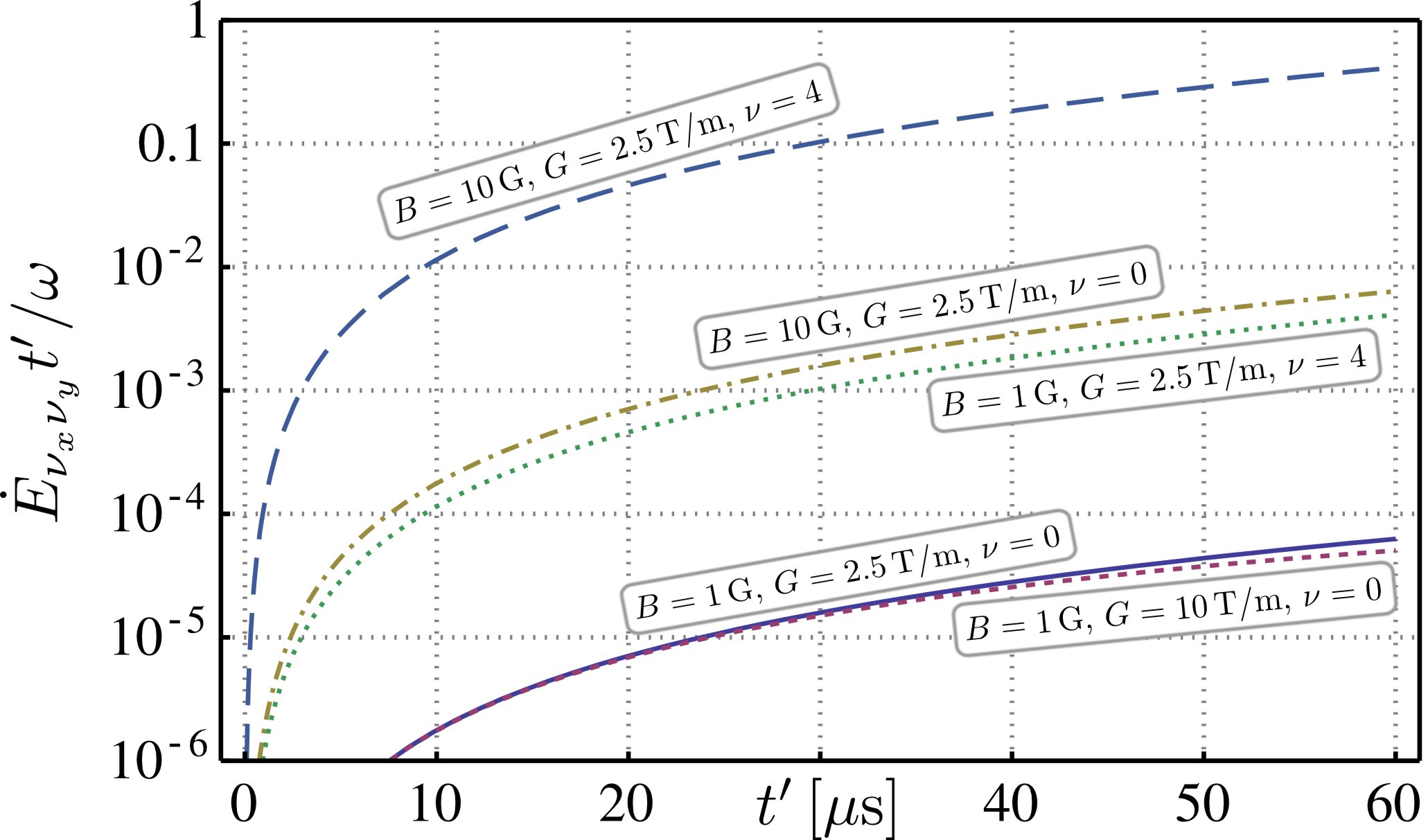
Figure 6: (Color online) Parametric heating $\dot{E}_{\nu_{x}\nu_{y}}t^{\prime}/\omega$ of a trapped ground state atom as a function of the time being excited to the Rydberg level $40S_{1/2}$. Several initial c.m. states and magnetic field configurations are considered: $B=1\,$G, $G=2.5\,$T/m (solid), $B=1\,$G, $G=10\,$T/m (short-dashed), and $B=10\,$G, $G=2.5\,$T/m (dashed-dotted) for $\nu_{x}=\nu_{y}=0$ as well as $B=1\,$G, $G=2.5\,$T/m (dotted) and $B=10\,$G, $G=2.5\,$T/m (long-dashed) for $\nu_{x}=\nu_{y}=2$.

VII Dephasing

Besides the parametric heating due to the short-time Rydberg excitation of a ground state atom – as discussed in the previous section – the dephasing of the c.m. motion of the Rydberg and the ground state might become an issue for experimental schemes realizing quantum information protocols. Let us consider the situation as described in Ref. Jaksch et al. (2000), i.e., we have two ground states denoted by $|0\rangle$ and $|1\rangle$ where only the latter is coupled to a Rydberg state $|r\rangle$ by a laser transition. The density operator of the internal degree of freedom, i.e., only considering the electronic state, of such a two state system can generally be written as $\rho_{\mathrm{int}}=a|0\rangle\langle 0|+(1-a)|1\rangle\langle 1|+b|1\rangle\langle 0|+b^{*}|0\rangle\langle 1|$ giving rise to the density matrix

$$\rho_{\mathrm{int}}=\begin{pmatrix}a&b^{*}\\ b&1-a\end{pmatrix}\,.$$ (35)

If we assume furthermore that both ground states are identically prepared with respect to their external, i.e., c.m. motion, the total density matrix factorizes into an internal and external contribution, $\rho_{\mathrm{tot}}=\rho_{\mathrm{int}}\otimes\rho_{\mathrm{ext}}$, where $\rho_{\mathrm{ext}}=\sum_{\nu_{y}\nu_{y}}p_{\nu_{x}\nu_{y}}|\nu_{x}\nu_{y}\rangle\langle\nu_{x}\nu_{y}|$.

For various implementations of quantum information protocols now the Rydberg state $|r\rangle$ comes into play. Suppose that state $|1\rangle$ is excited to $|r\rangle$ for a given time $t^{\prime}$. As pointed out in Sec. VI, this will influence its c.m. motion by causing transitions $|\nu_{x}\nu_{y}\rangle\rightarrow|\tilde{\chi}\rangle$, where $|\tilde{\chi}\rangle\equiv\sum_{\nu_{x}^{\prime}\nu_{y}^{\prime}}C_{\nu_{x}\nu_{y}}^{\nu_{x}^{\prime}\nu_{y}^{\prime}}(t^{\prime})|\nu_{x}^{\prime}\nu_{y}^{\prime}\rangle$; $C_{\nu_{x}\nu_{y}}^{\nu_{x}^{\prime}\nu_{y}^{\prime}}(t^{\prime})$ denotes the amplitude for being at time $t^{\prime}$ in state $|\nu_{x}^{\prime}\nu_{y}^{\prime}\rangle$ if initially residing in state $|\nu_{x}\nu_{y}\rangle$. Hence, after the short-time Rydberg excitation of solely state $|1\rangle$, the density matrix does not decouple anymore and consequently reads

$$\rho_{\mathrm{tot}}={} \sum_{\nu_{x}\nu_{y}}p_{\nu_{x}\nu_{y}}\big{[}a|0\rangle\langle 0|\otimes|\nu_{x}\nu_{y}\rangle\langle\nu_{x}\nu_{y}|$$

$$\qquad+(1-a)|1\rangle\langle 1|\otimes|\tilde{\chi}\rangle\langle\tilde{\chi}|$$

$$\qquad+b|1\rangle\langle 0|\otimes|\tilde{\chi}\rangle\langle\nu_{x}\nu_{y}|$$

$$\qquad+b^{*}|0\rangle\langle 1|\otimes|\nu_{x}\nu_{y}\rangle\langle\tilde{\chi}|\big{]}.$$ (36)

Any qubit-related measurement, however, only acts on the internal degrees of freedom, i.e., the electronic states. As a consequence, the relevant object in this case is the reduced density matrix where the c.m. degree of freedom is traced out. Defining $\beta=\sum_{\nu_{x}\nu_{y}}p_{\nu_{x}\nu_{y}}\langle\nu_{x}\nu_{y}|\tilde{\chi}\rangle$, one eventually yields

$$\mathrm{Tr}_{\mathrm{ext}}\rho_{\mathrm{tot}}=\begin{pmatrix}a&b^{*}\beta^{*}\\ b\beta&1-a\end{pmatrix}\,.$$ (37)

Comparing this result to the case where the internal and external degree of freedom factorize, $\mathrm{Tr}_{\mathrm{ext}}(\rho_{\mathrm{int}}\otimes\rho_{\mathrm{ext}})=\rho_{\mathrm{int}}$, it is clear that the short-time Rydberg excitation will inevitably influence the properties of our system. In order to quantify this effect, we consider the purity $\mathcal{P}(\rho)=\mathrm{Tr}\rho^{2}$ of the reduced density matrix. In particular, if the system is initially prepared in a pure internal state (as for example $(|0\rangle\pm|1\rangle)/\sqrt{2}$, which is envisaged for the realization of a two qubit cnot gate Urban et al. (2009)) the above described process is expected to decrease its purity. Indeed, one yields

$$\mathcal{P}(\mathrm{Tr}_{\mathrm{ext}}\rho_{\mathrm{tot}}) =a^{2}+(1-a)^{2}+2|b|^{2}|\beta|^{2}$$ (38)

$$=\mathcal{P}_{\mathrm{int}}-2|b|^{2}(1-|\beta|^{2})$$ (39)

where $\mathcal{P}_{\mathrm{int}}=a^{2}+(1-a)^{2}+2|b|^{2}$ denotes the purity of the system only considering the internal degree of freedom. Note that for any pure state $\mathcal{P}_{\mathrm{int}}=1$ is found. Hence, the reduction of the purity is determined by the magnitude of $|\beta|^{2}$ and therefore by the overlap integrals $\langle\nu_{x}\nu_{y}|\tilde{\chi}\rangle$ of the c.m. wavefunction after the Rydberg excitation.

A particularly illustrative situation arises, if the atom is initially prepared in its c.m. ground state, i.e., $p_{\nu_{x}\nu_{y}}=\delta_{0\nu_{x}}\delta_{0\nu_{y}}$ and $|\beta|^{2}=|\langle 00|\tilde{\chi}\rangle|^{2}$ correspondingly. In this case, $|\beta|^{2}$ is given by the probability of finding the atom still in the c.m. ground state after being excited to the Rydberg state for the time $t^{\prime}$. According to Sec. VI, we find

$$|\beta|^{2} =1-\sum_{\nu_{x}\nu_{y}\neq 00}W_{00\rightarrow\nu_{x}\nu_{y}}$$ (40)

$$=1-\frac{C_{z}^{2}G^{4}}{4M^{4}\omega^{4}}\left(\frac{\sin^{2}(\omega t^{\prime})}{\omega^{2}}+\frac{\sin^{2}(2\omega t^{\prime})}{4\omega^{2}}\right)$$ (41)

$$\approx 1-\frac{C_{z}^{2}G^{4}}{2M^{4}\omega^{4}}{t^{\prime}}^{2}$$ (42)

and therefore

$$\mathcal{P}(\mathrm{Tr}_{\mathrm{ext}}\rho_{\mathrm{tot}})\approx\mathcal{P}_{\mathrm{int}}-2|b|^{2}\frac{C_{z}^{2}G^{4}}{2M^{4}\omega^{4}}{t^{\prime}}^{2}\,.$$ (43)

As expected, the decrease of the purity depends explicitly (for short times $t^{\prime}$ even quadratically) on the time $t^{\prime}$ of being excited to the Rydberg level.

VIII Conclusion

We theoretically investigated the quantum properties of Rydberg atoms in a magnetic Ioffe-Pritchard trap. In particular, the electronic properties and the center of mass dynamics of the low angular momentum $nS$, $nP$, and $nD$ states of ⁸⁷Rb have been studied. It turns out that the composite nature of Rydberg atoms, i.e., the fact that it consists of an outer electron far away from a compact ionic core, significantly alters the coupling of the electronic motion to the inhomogeneous magnetic field of the Ioffe-Pritchard trap. We demonstrated that this leads to qualitative changes in the trapping potentials, namely, the appearance of an de-confining contribution which reduces the azimuthal symmetry to ${\bm{C}}_{4v}$. As a consequence, the resulting energy surfaces – which characterize the trapping potentials – possess a finite depth. Analytical expressions describing the surfaces were derived and the applicability of the applied perturbative treatment has been verified for experimentally relevant field strengths by comparison with numerical solutions of the underlying Schrödinger equation. Exemplary energy surfaces of the fully polarized $n=40$, $l=0,1,2$, $m_{j}=j$ states for the magnetic field configuration $B=1$ G, $G=2.5$ T/m were provided. A clear deviation from the harmonic confinement of a point-like particle with a trap depth of only a few vibrational quanta could be observed. Choosing different magnetic field parameters, on the other hand, trapping can be achieved with trap depths in the micro-Kelvin regime. The non-harmonicity of the Rydberg trapping potential becomes also apparent in the resulting center of mass dynamics: The additional contribution due to the two-body character of the Rydberg atom mixes the “unperturbed” harmonic eigenstates and thereby partially lifts their degeneracy. For an atom in its electronic ground state that is excited to a Rydberg state only for a short period of time, this provides a mechanism for parametric heating by populating excited center of mass states. The corresponding heating rate as a function of the initial center of mass state of the ground state atom has been derived. In the framework of quantum information protocols involving the short-time population of Rydberg atoms, it has been demonstrated that the same mechanism can lead to a decrease of the purity of the involved qubit states.

A rather natural extension of the present work would be the investigation of magnetic field configurations other than the Ioffe-Pritchard trap. For example, it is expected also in the case of a three-dimensional quadrupole field that similar terms associated with the composite nature of the Rydberg atom arise, significantly altering the trapping potential compared to the point-like particle description.