Spherical Distribution of 5 Points with Maximal Distance Sum

Abstract

In this paper, we mainly consider the problem of spherical distribution of 5 points, that is, how to configure 5 points on a sphere such that the mutual distance sum attains the maximum. It is conjectured that the sum of distances is maximal if 5 points form a bipyramid configuration in which case two points are positioned at two poles of the sphere and the other three are positioned uniformly on the equator. We study this problem using interval methods and related technics, and give a proof for the conjecture through computers in finite time.

1 Introduction

Studies on the problem of optimally arranging points on a sphere can date back to over one hundred years ago, when Thomson attempted to explain the periodic table in terms of the “plum pudding” model of the atom. Since then, several varied problems were proposed, and some of such problems are still unsolved now [1]. In general, these problems involve finding configurations of points on the surface of a sphere that maximize or minimize some given quantities, some of them are directly relevant to physics or chemistry where stable configurations tend to minimize some form of energy expression.

The problem has the following general form. Let $x_{1},x_{2},\ldots,x_{n}$ be points on the unit sphere $S^{m-1}$ of the Euclidean space $\mathbb{R}^{m}$, denote

$$V(X_{n},m,\lambda)=\sum\limits_{1\leq i<j\leq n}\left|x_{i}-x_{j}\right|^{\lambda},$$ (1.1)

where $X_{n}=(x_{1},x_{2},\ldots,x_{n})$, and $\left|x_{i}-x_{j}\right|$ denotes the Euclidean distance between $x_{i}$ and $x_{j}$.

For $\lambda\leq 0$, denote

$$V_{1}(n,m,\lambda)=\min\limits_{X_{n}\subset S^{m-1}}V(X,n,m,\lambda)$$ (1.2)

where

$$V_{1}(n,m,0)=\min\limits_{X_{n}\subset S^{m-1}}\sum\limits_{1\leq i<j\leq n}\log\frac{1}{\left|x_{i}-x_{j}\right|}$$ (1.3)

When $m=3$, this is the 7th Problem listed by Steve Smale in Mathematical Problems for the Next Century [2, 3].

For $\lambda>0$, denote

$$V_{2}(n,m,\lambda)=\max\limits_{X_{n}\subset S^{m-1}}V(X,n,m,\lambda)$$ (1.4)

So far as we know, G. Pólya and G. Szegö [4] first studied problems of such types in 1930s, since then, a number of results about $V_{2}(n,m,\lambda)$ have been derived. For example, L. Fejes Tóth proved results for cases when $m=2,\lambda=1$ and when $n=m+1,\lambda=1$ [6]. E. Hille considered the asymptotic properties of $V_{2}(n,m,\lambda)/N$ when $n\to\infty$ for definite $m$ and $\lambda$, and gave some results [7]. K. B. Stolarsky proved bounds of $V_{2}(n,m,\lambda)$ for definite $m$ and $\lambda$ in [8, 9], and gave some properties of point distributions corresponding $V_{2}(n,m,\lambda)$ when $m=2$ and $m=3$ in [10, 11, 12]. R. Alexander also proved bounds of $V_{2}(n,3,1)$ in [13], and discussed some generalized sums of distances in [14, 15]. G. D. Chakerian and M. S. Klamkin proved bounds of $V_{2}(n,m,1)$ in [16]. J. Berman and K. Hanes proved a property of the point distribution corresponding $V_{2}(n,3,1)$, and deduced some numerical results in [17]. G. Harman, J. Beck, T. Amdeberhan proved bounds of $V_{2}(n,m,\lambda)$ in [18, 19, 24]. Similar problems were also discussed in [20, 21, 22, 23].

For $V_{2}(5,3,1)$, numerical computations show evidences for the conjecture that, it is obtained when 5 points form a bipyramid configuration in which case two points are on the two poles of $S^{2}$, while three other points are uniformly distributed on the equator. In this paper, we study this problem via interval arithmetic, and prove the conjecture through computer in comparatively short time. For related problems, this guides a different method.

The main ideal of our proof is as follows. Firstly we express $V(X_{5},3,1)$ as a function under certain coordinate system, secondly we exclude a domain where the bipyramid configuration is proved to correspond an only maximum of $V(X_{5},3,1)$, lastly we subdivide the remaining domain, and prove that function values in these subdomains are less then the previous maximum obtained. So we complete the proof of the conjecture.

2 Mathematical descriptions of the problem

2.1 Spherical coordinate system

We choose the spherical coordinate system as showed in Fig. 1. A point $P$ on $S^{2}$ is identified by $(1,\phi,\theta)$, where $\phi\in\left[-\frac{\pi}{2},\frac{\pi}{2}\right]$ is the angle from vector $\overrightarrow{OH}$, i.e., the projection of vector $\overrightarrow{OP}$ in $xoy$-plane, to vector $\overrightarrow{OP}$, positive if the $z$-coordinate of $P$ is positive, and $\theta\in[-\pi,\pi)$ is the angle from $x$-axis to vector $\overrightarrow{OH}$, positive if the $y$-coordinate of $P$ is positive.

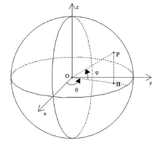
Fig. 1: The spherical coordinate system

According to such definitions, we have following formulas transforming from spherical coordinate $(1,\phi,\theta)$ to Cartesian coordinate $(x,y,z)$,

$$\left\{\begin{array}[]{rcl}x&=&\cos(\phi)\cos(\theta),\\ y&=&\cos(\phi)\sin(\theta),\\ z&=&\sin(\phi).\end{array}\right.$$ (2.1)

Considering the spherical symmetry, we can choose the spherical coordinates for 5 points as follows:

$$A(1,0,0),B(1,\phi_{1},\pi),C(1,\phi_{2},\theta_{2}),D(1,\phi_{3},\theta_{3}),E(1,\phi_{4},\theta_{4}).$$ (2.2)

Thus the sum of mutual distances of these points is

$$\begin{split}&f(\phi_{1},\phi_{2},\theta_{2},\phi_{3},\theta_{3},\phi_{4},\theta_{4})\\ =&\sqrt{2+2\,\cos\left(\phi_{{1}}\right)}+\sqrt{2-2\,\cos\left(\phi_{{2}}\right)\cos\left(\theta_{{2}}\right)}\\ &+\sqrt{2-2\,\cos\left(\phi_{{3}}\right)\cos\left(\theta_{{3}}\right)}+\sqrt{2-2\,\cos\left(\phi_{{4}}\right)\cos\left(\theta_{{4}}\right)}\\ &+\sqrt{2\,\cos\left(\phi_{{1}}\right)\cos\left(\phi_{{2}}\right)\cos\left(\theta_{{2}}\right)+2-2\,\sin\left(\phi_{{1}}\right)\sin\left(\phi_{{2}}\right)}\\ &+\sqrt{2\,\cos\left(\phi_{{1}}\right)\cos\left(\phi_{{3}}\right)\cos\left(\theta_{{3}}\right)+2-2\,\sin\left(\phi_{{1}}\right)\sin\left(\phi_{{3}}\right)}\\ &+\sqrt{2\,\cos\left(\phi_{{1}}\right)\cos\left(\phi_{{4}}\right)\cos\left(\theta_{{4}}\right)+2-2\,\sin\left(\phi_{{1}}\right)\sin\left(\phi_{{4}}\right)}\\ &+\sqrt{-2\,\cos\left(\phi_{{3}}\right)\cos\left(\phi_{{2}}\right)\cos\left(\theta_{{2}}-\theta_{{3}}\right)+2-2\,\sin\left(\phi_{{2}}\right)\sin\left(\phi_{{3}}\right)}\\ &+\sqrt{-2\,\cos\left(\phi_{{2}}\right)\cos\left(\phi_{{4}}\right)\cos\left(\theta_{{2}}-\theta_{{4}}\right)+2-2\,\sin\left(\phi_{{2}}\right)\sin\left(\phi_{{4}}\right)}\\ &+\sqrt{-2\,\cos\left(\phi_{{3}}\right)\cos\left(\phi_{{4}}\right)\cos\left(\theta_{{3}}-\theta_{{4}}\right)+2-2\,\sin\left(\phi_{{3}}\right)\sin\left(\phi_{{4}}\right)}.\end{split}$$ (2.3)

2.2 Bipyramid distribution

Spherical coordinates of 5 points corresponding a bipyramid distribution are not unique, but the following 5 points indeed form a bipyramid configuration,

$$A(1,0,0),B(1,-\dfrac{\pi}{3},\pi),C(1,\dfrac{\pi}{3},\pi),D(1,0,-\dfrac{\pi}{2}),E(1,0,\dfrac{\pi}{2}),$$ (2.4)

as showed in Fig. 2.

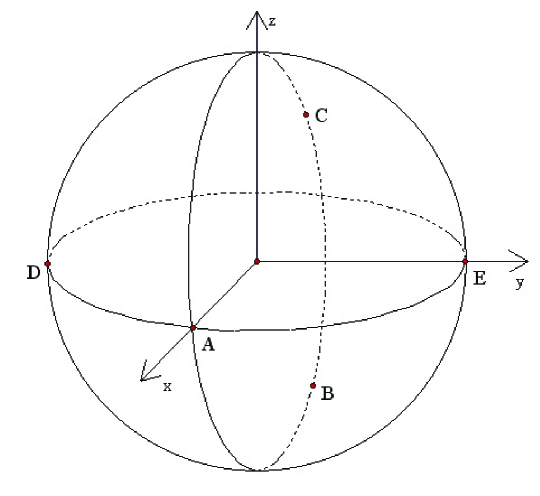
Fig. 2: The bipyramid distribution

Denote the corresponding values of $(\phi_{1},\phi_{2},\theta_{2},\phi_{3},\theta_{3},\phi_{4},\theta_{4})$ by

$$\Theta_{bp}=(-\dfrac{\pi}{3},\dfrac{\pi}{3},\pi,0,-\dfrac{\pi}{2},0,\dfrac{\pi}{2}),$$

then the corresponding value of function $f$ is

$$\begin{split}fmax&=f(\Theta_{bp})\\ &=3\,\sqrt{3}+6\,\sqrt{2}+2\\ &\approx 15.68143380,\end{split}$$ (2.5)

and the Hessian matrix of $f$ is

$$\left(\begin{array}[]{ccccccc}{\dfrac{-\sqrt{3}}{2}}&{\dfrac{\sqrt{3}}{4}}&0&{\dfrac{-\sqrt{2}}{4}}&{\dfrac{\sqrt{6}}{4}}&{\dfrac{-\sqrt{2}}{4}}&{\dfrac{-\sqrt{6}}{4}}\\ \vskip 6.0pt plus 2.0pt minus 2.0pt\cr{\dfrac{\sqrt{3}}{4}}&{\dfrac{-\sqrt{3}}{2}}&0&{\dfrac{-\sqrt{2}}{4}}&{\dfrac{-\sqrt{6}}{4}}&{\dfrac{-\sqrt{2}}{4}}&{\dfrac{\sqrt{6}}{4}}\\ \vskip 6.0pt plus 2.0pt minus 2.0pt\cr 0&0&{\dfrac{-2\,\sqrt{3}-3\,\sqrt{2}}{24}}&{\dfrac{-\sqrt{6}}{16}}&{\dfrac{\sqrt{2}}{16}}&{\dfrac{\sqrt{6}}{16}}&{\dfrac{\sqrt{2}}{16}}\\ \vskip 6.0pt plus 2.0pt minus 2.0pt\cr{\dfrac{-\sqrt{2}}{4}}&{\dfrac{-\sqrt{2}}{4}}&{\dfrac{-\sqrt{6}}{16}}&{\dfrac{-3\,\sqrt{2}-4}{8}}&0&{\dfrac{-1}{2}}&0\\ \vskip 6.0pt plus 2.0pt minus 2.0pt\cr{\dfrac{\sqrt{6}}{4}}&{\dfrac{-\sqrt{6}}{4}}&{\dfrac{\sqrt{2}}{16}}&0&{\dfrac{-3\,\sqrt{2}-4}{8}}&0&{\dfrac{1}{2}}\\ \vskip 6.0pt plus 2.0pt minus 2.0pt\cr{\dfrac{-\sqrt{2}}{4}}&{\dfrac{-\sqrt{2}}{4}}&{\dfrac{\sqrt{6}}{16}}&{\dfrac{-1}{2}}&0&{\dfrac{-3\,\sqrt{2}-4}{8}}&0\\ \vskip 6.0pt plus 2.0pt minus 2.0pt\cr{\dfrac{-\sqrt{6}}{4}}&{\dfrac{\sqrt{6}}{4}}&{\dfrac{\sqrt{2}}{16}}&0&{\dfrac{1}{2}}&0&{\dfrac{-3\,\sqrt{2}-4}{8}}\end{array}\right).$$ (2.6)

This matrix is negative definite, so the bipyramid distribution corresponds a maximum of function $f$.

2.3 Inequality form

As a matter of fact, what we are to prove is the following inequality,

$$f(\phi_{1},\phi_{2},\theta_{2},\phi_{3},\theta_{3},\phi_{4},\theta_{4})\leq fmax,\quad(\phi_{1},\phi_{2},\theta_{2},\phi_{3},\theta_{3},\phi_{4},\theta_{4})\in\mathcal{D}.$$ (2.7)

where

$$\mathcal{D}=\left([-\frac{\pi}{2},\frac{\pi}{2}],[-\frac{\pi}{2},\frac{\pi}{2}],[-\pi,\pi),[-\frac{\pi}{2},\frac{\pi}{2}],[-\pi,\pi),[-\frac{\pi}{2},\frac{\pi}{2}],[-\pi,\pi)\right),$$

and the equality holds if and only if $(\phi_{1},\phi_{2},\theta_{2},\phi_{3},\theta_{3},\phi_{4},\theta_{4})=\Theta_{bp}$.

In the remaining part of this paper, we will according to following steps to prove this inequality.

1. Giving some restricted conditions and results to demonstrate that we only need to prove the inequality over a subdomain of $\mathcal{D}$, i.e., $\mathcal{D}^{(1)}\cup\mathcal{D}^{(2)}$ (see Eq. (4.6)).

2. Analyzing interval Hessian matrices (Theorem 4.3, 4.4 and 4.6) to prove that the equality holds only at $\Theta_{bp}$ over a subdomain of $\mathcal{D}^{(1)}\cup\mathcal{D}^{(2)}$, i.e., $\mathcal{D}_{bp}$ (see Proposition 4.1).

3. Analyzing interval Hessian matrices (Theorem 4.5 and 4.7) to prove the corresponding strict inequality holds over a subdomain of $\mathcal{D}^{(1)}\cup\mathcal{D}^{(2)}$, i.e., $\mathcal{D}_{p}$ (see Proposition 5.1).

4. Making use of the interval arithmetic(§ 4.1.1) to prove the corresponding strict inequality holds over the remaining domains, i.e., $(\mathcal{D}^{(1)}\cup\mathcal{D}^{(2)})\backslash(\mathcal{D}_{bp}\cup\mathcal{D}_{p})$ (see Eq. (6.1)).

3 Restricted conditions and verification domain

3.1 Some results

What we are to prove is in fact that, there exists no distribution of 5 points exclude the bipyramid distribution corresponding larger distance sum then $fmax$. We need following results so as to simplify this problem.

Proposition 3.1.

If some configuration of 5 points corresponds larger function value of $f$ then the bipyramid configuration, and $AB$ is the second largest distance in ${5\choose 2}=10$ distances, $\phi_{1}$ should satisfy

$$\phi_{1}\geq-2\,\arccos(\sqrt{3}/6+\sqrt{2}/3)$$ (3.1)

Proof.

From Equation (2.5), we know that in order to attain larger distance sum than that the bipyramid configuration corresponds, the second largest distance must be not smaller then

$$((3\,\sqrt{3}+6\,\sqrt{2}+2)-2)/9=\sqrt{3}/3+2\,\sqrt{2}/3.$$

With the condition that $AB$ is the second largest distance, the result required can be deduced immediately. ∎

Proposition 3.2.

If 5 points are on the same half sphere, $f$ can not attains its maximum.

Proof.

Without loss of generality, suppose $z$-coordinates of 5 points are all nonpositive, if the $z$-coordinate of some point is negative, we move it to the symmetric position with respect to the $xoy$-plane, then we will get a larger distance sum.

If 5 points are all distributed on the $xoy$-plane, the maximal distance sum is [6] (5 points form a regular pentagon) $5\,\cot\frac{\pi}{10}$, which is obviously smaller then the mutual distance sum corresponding the bipyramid configuration (see § 2.2). ∎

Proposition 3.3.

If a partial derivative of function $f$ does not vary signs in a domain, then there exists no stationary point of $f$ in this domain.

Theorem 3.1.

[17] Let $p_{1},\ldots,p_{n}$ be points on the unit sphere $S^{2}$ in $\mathbb{R}^{3}$. Let $f:\,S^{2}\to\mathbb{R}$ be defined by $f(x)=\sum\limits_{i=1}^{n}\left|x-p_{i}\right|$. if $f$ has a maximum at $p$, then $p=q/|q|$, where $q=\sum\limits_{i=1}^{n}(p-p_{i})/\left|p-p_{i}\right|$.

Theorem 3.2.

[8] Suppose the 5 points are placed so that function $f$ is maximal, then any distance between two points cannot be less then $\frac{2}{15}$.

3.2 Some restricted conditions

We can consider the problem under following restricted conditions due to above results.

Condition 3.1.

$AB$ is the second largest distance in ${5\choose 2}=10$ distances.

Condition 3.2.

$D$ is on the left half sphere, $C,E$ are on the right half sphere, $C$ is above $E$.

Condition 3.3 (by Proposition 3.1).

$\phi_{1}\geq-2\,\arccos(\sqrt{3}/6+\sqrt{2}/3)$

Condition 3.4 (by Proposition 3.2).

Five points are not on any half sphere.

Condition 3.5 (by Theorem 3.2).

Distances between any two points are larger then $\frac{2}{15}$.

3.3 Domain subdivision

Under these conditions, the bipyramid configuration (corresponding the maximal distance sum conjectured) and the pyramid configuration (corresponding another stationary point of the function $f$) each corresponds only one coordinate representation. Further more, we can divide the domain in which we need to verify no distribution of points corresponds a larger distance sum into the following two subdomains:

1. $D$ is on the upper half sphere (denote this domain by $\mathcal{D}^{(1)}$):

   $\begin{array}[]{l}\phi_{{1}}\in[-2\,\arccos\left(\sqrt{3}/6+\sqrt{2}/3\right),0],\\ \phi_{{2}}\in[-\pi/2,0],\\ \theta_{{2}}\in[0,\pi],\\ \phi_{{3}}\in[0,\pi/2],\\ \theta_{{3}}\in[-\pi,0],\\ \phi_{{4}}\in[-\pi/2,0],\\ \theta_{{4}}\in[0,\pi].\end{array}$

2. $D$ is on the lower half sphere, $C$ is on the upper half sphere (denote this domain by $\mathcal{D}^{(2)}$):

   $\begin{array}[]{l}\phi_{{1}}\in[-2\,\arccos\left(\sqrt{3}/6+\sqrt{2}/3\right),0],\\ \phi_{{2}}\in[0,\pi/2],\\ \theta_{{2}}\in[0,\pi],\\ \phi_{{3}}\in[-\pi/2,\pi/2],\\ \theta_{{3}}\in[-\pi,0],\\ \phi_{{4}}\in[-\pi/2,\pi/2],\\ \theta_{{4}}\in[0,\pi].\end{array}$

Now, we are to prove that, under Condition 3.1 - 3.5, function $f$ attains its maximum in $\mathcal{D}^{(1)}$ and $\mathcal{D}^{(2)}$ at the only point corresponding the bipyramid distribution of $A,B,C,D,E$, i.e.,

$$f(\phi_{1},\phi_{2},\theta_{2},\phi_{3},\theta_{3},\phi_{4},\theta_{4})\leq fmax,\quad(\phi_{1},\phi_{2},\theta_{2},\phi_{3},\theta_{3},\phi_{4},\theta_{4})\in\mathcal{D}^{(1)}\cup\mathcal{D}^{(2)}.$$ (3.2)

where the equality holds if and only if $(\phi_{1},\phi_{2},\theta_{2},\phi_{3},\theta_{3},\phi_{4},\theta_{4})=\Theta_{bp}$.

In the following parts of this paper, we will illustrate the domain verification methods, and detailed steps as well as results.

4 Domain near coordinates corresponding the bipyramid distribution

4.1 Interval methods

We first briefly introduce the interval methods we used in our proof.

4.1.1 Interval arithmetic

We define an interval as a set [25]:

$$X=[a,b]=\{x:a\leq x\leq b\},$$ (4.1)

where $a,b\in\mathbb{R}$. $\underline{X},\overline{X}$ respectively denote the left and right vertexes of the interval $X$.

For intervals $X$ and $Y$, if $x>y$ for each $x\in X$ and each $y\in Y$, we say that $X>Y$. Other interval relations are understood the same way. An $n$-dimensional “interval vector” is an $n$-tuple of intervals $\mathbf{X}=(X_{1},\ldots,X_{n})$, which is used to denote some rectangular domain in $\mathbb{R}^{n}$. Let $\mathbb{IR}$ be the set of intervals over $\mathbb{R}$, and $\mathbb{IR}^{n}$ be the set of $n$-dimensional “interval vectors”.

We can define an imbedding from $\mathbb{R}$ to $\mathbb{IR}$ as follows

$$\mu(x)=[x,x],$$

thus for numbers in $\mathbb{R}$, we can also consider them as intervals.

We define interval arithmetic over $\mathbb{IR}$ as

$$X\circ Y=\{x\circ y:x\in X,y\in Y\},$$

where $\circ$ is $``+",``-",``*"$ or $``/"$. Further more, for an elementary function $f$, we define a corresponding elementary mapping as

$$f(X)=\{f(x):x\in X\}.$$

When operands of interval arithmetic or arguments of elementary functions are intervals, we consider underlying computations are interval computations defined above, and the interval computation is of the same precedence as the corresponding arithmetic computation.

Under above definitions, an arbitrary elementary function $f:\mathbb{R}^{n}\to\mathbb{R}$ can be expanded to a mapping over $\mathbb{IR}^{n}\to\mathbb{IR}$:

$$\tilde{f}(\mathbf{X})=f(\mathbf{X}).$$ (4.2)

Through such $\tilde{f}$, We can get an interval which contains the function range of $f$ over rectangular domain $\mathbf{X}$, this is the critical point we solve the problem.

As a matter of fact, there are related programs used to process interval arithmetic, such as the procedure evalr can be used to implement interval arithmetic without errors. But in practice, it may be not necessary to implement errorless interval arithmetic, because what we get from interval arithmetic are just intervals contains the ranges of function values. Another problem is that acting such errorless interval arithmetic is always time-consuming, thus it cannot meet our needs.

Considering the efficiency and the accuracy, we wrote an interval arithmetic package IntervalArithmetic based on the Maple system. The package uses rational numbers as interval vertexes, and acts computations with controllable errors. In fact the result it computes for $f(\mathbf{X})$ is an larger interval containing $\tilde{f}(\mathbf{X})$, and the difference can reduce to zero as intervals of $\mathbf{X}$ shrink to points. For the detailed code, see Appendix A.1.

4.1.2 Interval matrices

Relations of real matrices of the same order are understood componentwise. An interval matrix is defined as the following set of matrices:

$$([\underline{a}_{ij},\overline{a}_{ij}])=[\underline{A},\overline{A}]=\{A\in\mathbb{R}^{n\,\times\,n}:\underline{A}\leq A\leq\overline{A}\},$$

where

$$\underline{A}=(\underline{a}_{ij}),\overline{A}=(\overline{a}_{ij}).$$

When $\underline{A}$ and $\overline{A}$ are symmetric, we call the set of symmetric matrices in $[\underline{A},\overline{A}]$ a symmetric interval matrix which is also denoted by $[\underline{A},\overline{A}]$.

For a interval matrix $[\underline{A},\overline{A}]$, denote its midpoint matrix by $A_{c}=\dfrac{\underline{A}+\overline{A}}{2}$, radius matrix by $A_{\delta}=\dfrac{\overline{A}-\underline{A}}{2}$. For a real symmetric matrix $A$, it is well know that all its eigenvalues are real, we denote them in decreasing order by $\lambda_{1}(A)\geq\lambda_{2}(A)\geq\cdots\geq\lambda_{n}(A)$, and denote the spectrum of $A$ (i.e. the maximum eigenvalue modulus) by $\varrho(A)$. For bounds of eigenvalues of matrices in an interval matrix, it can be directly deduced from the Wielandt-Hoffman theorem [28] that

Theorem 4.1.

For a symmetric interval matrix $[\underline{A},\overline{A}]$, the set

$$\{\lambda_{i}(A):A\in[\underline{A},\overline{A}]\}$$

is a compact interval, denote this compact interval by

$$[\underline{\lambda}_{i}([\underline{A},\overline{A}]),\overline{\lambda}_{i}([\underline{A},\overline{A}])],\,1\leq i\leq n,$$

then

$$[\underline{\lambda}_{i}([\underline{A},\overline{A}]),\overline{\lambda}_{i}([\underline{A},\overline{A}])]\subseteq[\lambda_{i}(A_{c})-\varrho(A_{\delta}),\lambda_{i}(A_{c})+\varrho(A_{\delta})],\,i=1,\ldots,n.$$

In fact, $\overline{\lambda}_{1}([\underline{A},\overline{A}])$ and $\underline{\lambda}_{n}([\underline{A},\overline{A}])$ can be solved explicitly [26], that is,

Theorem 4.2.

A real symmetric interval matrix

$$([\underline{a}_{ij},\overline{a}_{ij}])=\{A\in\mathbb{R}^{n\,\times\,n}:\underline{A}\leq A\leq\overline{A},\underline{A}=(\underline{a}_{ij}),\overline{A}=(\overline{a}_{ij})\}$$

corresponds following $2^{n-1}$ vertex matrices:

$$A_{k}=(a_{kij}),0\leq k\leq 2^{n-1}-1,$$

where we denote the binary representation for $k$ by $k=(k_{1}k_{2}\cdots k_{n})_{2}$, and

$$a_{kij}=\frac{1}{2}(\underline{a}_{ij}+\overline{a}_{ij}+(-1)^{k_{i}+k_{j}}(\underline{a}_{ij}-\overline{a}_{ij})).$$

For matrices in this symmetric interval matrix, minimal (or maximal) eigenvalues of them attain the minimum (respectively, maximum) at some vertex matrix $A_{k}$.

For a real symmetric interval matrix $[\underline{A},\overline{A}]$, we say it is positive (semi)definite if $A$ is positive (semi)definite for each $A\in[\underline{A},\overline{A}]$, and it is nonpositive (semi)definite if $A$ is not positive (semi)definite for each $A\in[\underline{A},\overline{A}]$. Definitions such as negative (semi)definiteness, nonnegative (semi)definiteness of $[\underline{A},\overline{A}]$ are understood the similar way.

Now we introduce the results for verifying positive definiteness and nonpositive semidefiniteness of symmetric interval matrices, which can directly deduce criterions for negative definiteness, nonnegative definiteness, etc.

Rohn has given the following theorem [26], which is an improvement on results in [27], we state it in a varied way that adapts to be understood as an algorithm.

Theorem 4.3.

The real symmetric interval matrix

$$([\underline{a}_{ij},\overline{a}_{ij}])=\{A\in\mathbb{R}^{n\,\times\,n}:\underline{A}\leq A\leq\overline{A},\underline{A}=(\underline{a}_{ij}),\overline{A}=(\overline{a}_{ij})\}$$

is positive definite if and only if the following $2^{n-1}$ vertex matrices are all positive definite:

$$A_{k}=(a_{kij}),0\leq k\leq 2^{n-1}-1,$$

where we denote the binary representation for $k$ by $k=(k_{1}k_{2}\cdots k_{n})_{2}$, and

$$a_{kij}=\frac{1}{2}(\underline{a}_{ij}+\overline{a}_{ij}+(-1)^{k_{i}+k_{j}}(\underline{a}_{ij}-\overline{a}_{ij})).$$

Theorem 4.2 in fact implies Theorem 4.3, because the positive definiteness of a symmetric interval matrix is equal that the minimum of minimal eigenvalues of matrices in it is positive. So we can get from Theorem 4.1 a sufficient condition for determining the positive definiteness of a symmetric interval matrix.

Theorem 4.4.

The symmetric interval matrix $[\underline{A},\overline{A}]$ is positive definite if

$$\lambda_{n}(A_{c})-\varrho(A_{\delta})>0,$$

where $A_{c}$ and $A_{\delta}$ are the midpoint matrix and the radius matrix respectively.

Similarly, the nonpositive semidefiniteness of a symmetric interval matrix is equal that the maximum of minimal eigenvalues of matrices in it is negative, i.e.,

Theorem 4.5.

The symmetric interval matrix $[\underline{A},\overline{A}]$ is nonpositive semidefinite if

$$\lambda_{n}(A_{c})+\varrho(A_{\delta})<0,$$

where $A_{c}$ and $A_{\delta}$ are the midpoint matrix and the radius matrix respectively.

The procedure isdef in the package IntervalArithmetic can implement algorithms above to verify the properties of symmetric interval matrices, such as positive definiteness, negative definiteness and so on.

With the help of above theorems, we can use the following trivial results to determine the extreme point of a function in a domain.

Theorem 4.6.

If $g\in C^{2}(D)$, $X_{0}\in D$ is a stationary point of $g$, and the Hessian matrix of $g$ over $D$ varies in a positive definite real symmetric interval matrix, then $X_{0}$ is the minimum point of $g$ in $D$.

Theorem 4.7.

If $g\in C^{2}(D)$, and the Hessian matrix of $g$ over $D$ varies in a nonpositive semidefinite real symmetric interval matrix, then no inner point of $D$ is the minimum point of $g$.

4.2 Domain excluded near coordinates corresponding the bipyramid distribution

Now we introduce a disturbance $\left[-\frac{\pi}{377},\frac{\pi}{377}\right]$ on coordinates corresponding the bipyramid distribution, and obtain a rectangular domain, i.e.,

$$\left(\begin{array}[]{c}\phi_{{1}}\\ \vskip 6.0pt plus 2.0pt minus 2.0pt\cr\phi_{{2}}\\ \vskip 6.0pt plus 2.0pt minus 2.0pt\cr\theta_{{2}}\\ \vskip 6.0pt plus 2.0pt minus 2.0pt\cr\phi_{{3}}\\ \vskip 6.0pt plus 2.0pt minus 2.0pt\cr\theta_{{3}}\\ \vskip 6.0pt plus 2.0pt minus 2.0pt\cr\phi_{{4}}\\ \vskip 6.0pt plus 2.0pt minus 2.0pt\cr\theta_{{4}}\end{array}\right)\in\left(\begin{array}[]{c}\left[-{\frac{380}{1131}}\,\pi,-{\frac{374}{1131}}\,\pi\right]\\ \vskip 6.0pt plus 2.0pt minus 2.0pt\cr\left[{\frac{374}{1131}}\,\pi,{\frac{380}{1131}}\,\pi\right]\\ \vskip 6.0pt plus 2.0pt minus 2.0pt\cr\left[{\frac{376}{377}}\,\pi,{\frac{378}{377}}\,\pi\right]\\ \vskip 6.0pt plus 2.0pt minus 2.0pt\cr\left[-{\frac{1}{377}}\,\pi,{\frac{1}{377}}\,\pi\right]\\ \vskip 6.0pt plus 2.0pt minus 2.0pt\cr\left[-{\frac{379}{754}}\,\pi,-{\frac{375}{754}}\,\pi\right]\\ \vskip 6.0pt plus 2.0pt minus 2.0pt\cr\left[-{\frac{1}{377}}\,\pi,{\frac{1}{377}}\,\pi\right]\\ \vskip 6.0pt plus 2.0pt minus 2.0pt\cr\left[{\frac{375}{754}}\,\pi,{\frac{379}{754}}\,\pi\right]\end{array}\right).$$ (4.3)

In this domain, $\theta_{2}$ varies in $\left[{\frac{376}{377}}\,\pi,{\frac{378}{377}}\,\pi\right]$, which exceeds the bound we prescribed for $\theta_{2}$. But since the periodicity of function $f$, it is of no error. In fact, interval vertexes are represented by rational numbers in the Maple package IntervalArithmetic, so these intervals whose vertexes contain $\pi$ are enlarged to their rational representations, that is, the rectangular domain we actually obtain is

$$\mathcal{D}_{bp}=\left(\begin{array}[]{c}\left[-{\frac{1055530689}{1000000000}},-{\frac{1038864413}{1000000000}}\right]\\ \vskip 6.0pt plus 2.0pt minus 2.0pt\cr\left[{\frac{1038864413}{1000000000}},{\frac{1055530689}{1000000000}}\right]\\ \vskip 6.0pt plus 2.0pt minus 2.0pt\cr\left[{\frac{783314879}{250000000}},{\frac{98435181}{31250000}}\right]\\ \vskip 6.0pt plus 2.0pt minus 2.0pt\cr\left[-{\frac{10416421265218147343}{1250000000000000000000}},{\frac{10416421265218147343}{1250000000000000000000}}\right]\\ \vskip 6.0pt plus 2.0pt minus 2.0pt\cr\left[-{\frac{315825893}{200000000}},-{\frac{1562463189}{1000000000}}\right]\\ \vskip 6.0pt plus 2.0pt minus 2.0pt\cr\left[-{\frac{10416421265218147343}{1250000000000000000000}},{\frac{10416421265218147343}{1250000000000000000000}}\right]\\ \vskip 6.0pt plus 2.0pt minus 2.0pt\cr\left[{\frac{1562463189}{1000000000}},{\frac{315825893}{200000000}}\right]\end{array}\right).$$ (4.4)

The interval Hessian matrix of $f$ over $\mathcal{D}_{bp}$ can be calculated by interval arithmetic:

$$\mathcal{V}=\left(V_{1},V_{2},V_{3},V_{4},V_{5},V_{6},V_{7}\right),$$ (4.5)

where $V_{i}(i=1,\ldots,7)$ are vectors as follows:

$V_{{1}}=\left(\begin{array}[]{c}\left[-{\dfrac{9073071021}{10000000000}},-{\dfrac{257887557}{312500000}}\right]\\ \vskip 6.0pt plus 2.0pt minus 2.0pt\cr\left[{\dfrac{4158136493}{10000000000}},{\dfrac{1126402921}{2500000000}}\right]\\ \vskip 6.0pt plus 2.0pt minus 2.0pt\cr\left[-{\dfrac{2503191333}{1000000000000}},{\dfrac{2503191333}{1000000000000}}\right]\\ \vskip 6.0pt plus 2.0pt minus 2.0pt\cr\left[-{\dfrac{910889963}{2500000000}},-{\dfrac{428510269}{1250000000}}\right]\\ \vskip 6.0pt plus 2.0pt minus 2.0pt\cr\left[{\dfrac{6038013477}{10000000000}},{\dfrac{1552383121}{2500000000}}\right]\\ \vskip 6.0pt plus 2.0pt minus 2.0pt\cr\left[-{\dfrac{72871197}{200000000}},-{\dfrac{685616431}{2000000000}}\right]\\ \vskip 6.0pt plus 2.0pt minus 2.0pt\cr\left[-{\dfrac{3104766243}{5000000000}},-{\dfrac{6038013477}{10000000000}}\right]\end{array}\right),V_{{2}}=\left(\begin{array}[]{c}\left[{\dfrac{4158136493}{10000000000}},{\dfrac{1126402921}{2500000000}}\right]\\ \vskip 6.0pt plus 2.0pt minus 2.0pt\cr\left[-{\dfrac{2283824451}{2500000000}},-{\dfrac{8191611957}{10000000000}}\right]\\ \vskip 6.0pt plus 2.0pt minus 2.0pt\cr\left[-{\dfrac{23364423}{781250000}},{\dfrac{747661531}{25000000000}}\right]\\ \vskip 6.0pt plus 2.0pt minus 2.0pt\cr\left[-{\dfrac{114837637}{312500000}},-{\dfrac{3397366803}{10000000000}}\right]\\ \vskip 6.0pt plus 2.0pt minus 2.0pt\cr\left[-{\dfrac{1559063347}{2500000000}},-{\dfrac{240452637}{400000000}}\right]\\ \vskip 6.0pt plus 2.0pt minus 2.0pt\cr\left[-{\dfrac{183740219}{500000000}},-{\dfrac{424670851}{1250000000}}\right]\\ \vskip 6.0pt plus 2.0pt minus 2.0pt\cr\left[{\dfrac{6011315931}{10000000000}},{\dfrac{779531673}{1250000000}}\right]\end{array}\right)$
$V_{{3}}=\left(\begin{array}[]{c}\left[-{\dfrac{2503191333}{1000000000000}},{\dfrac{2503191333}{1000000000000}}\right]\\ \vskip 6.0pt plus 2.0pt minus 2.0pt\cr\left[-{\dfrac{23364423}{781250000}},{\dfrac{747661531}{25000000000}}\right]\\ \vskip 6.0pt plus 2.0pt minus 2.0pt\cr\left[-{\dfrac{3523502821}{10000000000}},-{\dfrac{2901860369}{10000000000}}\right]\\ \vskip 6.0pt plus 2.0pt minus 2.0pt\cr\left[-{\dfrac{1628135751}{10000000000}},-{\dfrac{359058763}{2500000000}}\right]\\ \vskip 6.0pt plus 2.0pt minus 2.0pt\cr\left[{\dfrac{1556247929}{20000000000}},{\dfrac{9916175537}{100000000000}}\right]\\ \vskip 6.0pt plus 2.0pt minus 2.0pt\cr\left[{\dfrac{718117527}{5000000000}},{\dfrac{1628135749}{10000000000}}\right]\\ \vskip 6.0pt plus 2.0pt minus 2.0pt\cr\left[{\dfrac{7781239691}{100000000000}},{\dfrac{2479043873}{25000000000}}\right]\end{array}\right),V_{{4}}=\left(\begin{array}[]{c}\left[-{\dfrac{910889963}{2500000000}},-{\dfrac{428510269}{1250000000}}\right]\\ \vskip 6.0pt plus 2.0pt minus 2.0pt\cr\left[-{\dfrac{114837637}{312500000}},-{\dfrac{3397366803}{10000000000}}\right]\\ \vskip 6.0pt plus 2.0pt minus 2.0pt\cr\left[-{\dfrac{1628135751}{10000000000}},-{\dfrac{359058763}{2500000000}}\right]\\ \vskip 6.0pt plus 2.0pt minus 2.0pt\cr\left[-{\dfrac{214384921}{200000000}},-{\dfrac{9891691177}{10000000000}}\right]\\ \vskip 6.0pt plus 2.0pt minus 2.0pt\cr\left[-{\dfrac{483991657}{20000000000}},{\dfrac{97153283}{4000000000}}\right]\\ \vskip 6.0pt plus 2.0pt minus 2.0pt\cr\left[-{\dfrac{10001389}{20000000}},-{\dfrac{4999305593}{10000000000}}\right]\\ \vskip 6.0pt plus 2.0pt minus 2.0pt\cr\left[-{\dfrac{1041678267}{10000000000000}},{\dfrac{1041678267}{10000000000000}}\right]\end{array}\right)$
$V_{{5}}=\left(\begin{array}[]{c}\left[{\dfrac{6038013477}{10000000000}},{\dfrac{1552383121}{2500000000}}\right]\\ \vskip 6.0pt plus 2.0pt minus 2.0pt\cr\left[-{\dfrac{1559063347}{2500000000}},-{\dfrac{240452637}{400000000}}\right]\\ \vskip 6.0pt plus 2.0pt minus 2.0pt\cr\left[{\dfrac{1556247929}{20000000000}},{\dfrac{9916175537}{100000000000}}\right]\\ \vskip 6.0pt plus 2.0pt minus 2.0pt\cr\left[-{\dfrac{483991657}{20000000000}},{\dfrac{97153283}{4000000000}}\right]\\ \vskip 6.0pt plus 2.0pt minus 2.0pt\cr\left[-{\dfrac{1058713931}{1000000000}},-{\dfrac{1002296947}{1000000000}}\right]\\ \vskip 6.0pt plus 2.0pt minus 2.0pt\cr\left[-{\dfrac{1041678267}{10000000000000}},{\dfrac{1041678267}{10000000000000}}\right]\\ \vskip 6.0pt plus 2.0pt minus 2.0pt\cr\left[{\dfrac{312434903}{625000000}},{\dfrac{1250173619}{2500000000}}\right]\end{array}\right),V_{{6}}=\left(\begin{array}[]{c}\left[-{\dfrac{72871197}{200000000}},-{\dfrac{685616431}{2000000000}}\right]\\ \vskip 6.0pt plus 2.0pt minus 2.0pt\cr\left[-{\dfrac{183740219}{500000000}},-{\dfrac{424670851}{1250000000}}\right]\\ \vskip 6.0pt plus 2.0pt minus 2.0pt\cr\left[{\dfrac{718117527}{5000000000}},{\dfrac{1628135749}{10000000000}}\right]\\ \vskip 6.0pt plus 2.0pt minus 2.0pt\cr\left[-{\dfrac{10001389}{20000000}},-{\dfrac{4999305593}{10000000000}}\right]\\ \vskip 6.0pt plus 2.0pt minus 2.0pt\cr\left[-{\dfrac{1041678267}{10000000000000}},{\dfrac{1041678267}{10000000000000}}\right]\\ \vskip 6.0pt plus 2.0pt minus 2.0pt\cr\left[-{\dfrac{1071924603}{1000000000}},-{\dfrac{2472922799}{2500000000}}\right]\\ \vskip 6.0pt plus 2.0pt minus 2.0pt\cr\left[-{\dfrac{607208011}{25000000000}},{\dfrac{302494783}{12500000000}}\right]\end{array}\right)$
$V_{{7}}=\left(\begin{array}[]{c}\left[-{\dfrac{3104766243}{5000000000}},-{\dfrac{6038013477}{10000000000}}\right]\\ \vskip 6.0pt plus 2.0pt minus 2.0pt\cr\left[{\dfrac{6011315931}{10000000000}},{\dfrac{779531673}{1250000000}}\right]\\ \vskip 6.0pt plus 2.0pt minus 2.0pt\cr\left[{\dfrac{7781239691}{100000000000}},{\dfrac{2479043873}{25000000000}}\right]\\ \vskip 6.0pt plus 2.0pt minus 2.0pt\cr\left[-{\dfrac{1041678267}{10000000000000}},{\dfrac{1041678267}{10000000000000}}\right]\\ \vskip 6.0pt plus 2.0pt minus 2.0pt\cr\left[{\dfrac{312434903}{625000000}},{\dfrac{1250173619}{2500000000}}\right]\\ \vskip 6.0pt plus 2.0pt minus 2.0pt\cr\left[-{\dfrac{607208011}{25000000000}},{\dfrac{302494783}{12500000000}}\right]\\ \vskip 6.0pt plus 2.0pt minus 2.0pt\cr\left[-{\dfrac{1058713929}{1000000000}},-{\dfrac{20045939}{20000000}}\right]\end{array}\right)$

Through Theorem 4.3, we can judge that the symmetric interval matrix $\mathcal{V}$ is negative definite, and by Theorem 4.6, the conjectured configuration indeed corresponds the maximum of $f$ in $\mathcal{D}_{bp}$. That is

Proposition 4.1.

The bipyramid distribution of 5 points represented by Eq. (2.4) is the only maximal distance sum distribution in domain $\mathcal{D}_{bp}$, i.e.,

$$f(\phi_{1},\phi_{2},\theta_{2},\phi_{3},\theta_{3},\phi_{4},\theta_{4})\leq fmax,\quad(\phi_{1},\phi_{2},\theta_{2},\phi_{3},\theta_{3},\phi_{4},\theta_{4})\in\mathcal{D}_{bp},$$ (4.6)

where the equality holds if and only if $(\phi_{1},\phi_{2},\theta_{2},\phi_{3},\theta_{3},\phi_{4},\theta_{4})=\Theta_{bp}$.

5 Domain near coordinates corresponding the pyramid distribution

Under conditions in § 3.2, coordinates representing the pyramid distribution are unique, while they corresponds a stationary point of function $f$, and the function value on this point is too close to $fmax$, therefore, we discuss it separately.

5.1 Pyramid distribution

The spherical coordinate corresponding the pyramid distribution is

$$\begin{array}[]{l}A(1,0,0),\\[5.0pt] B\left(1,-2\,\omega_{1},\pi\right),\\[5.0pt] C\left(1,\dfrac{\pi}{2}-\omega_{1},\pi\right),\\[5.0pt] D\left(1,\omega_{2},-\omega_{3}\right),\\[5.0pt] E\left(1,\omega_{2},\omega_{3}\right),\end{array}$$ (5.1)

where

$$\begin{split}\omega_{1}&=\arcsin\left(-\dfrac{3}{4}+\dfrac{\sqrt{2}}{2}+\dfrac{\sqrt{41-28\,\sqrt{2}}}{4}\right),\\ \omega_{2}&=-\arcsin\left(\left(-\dfrac{3}{4}+\dfrac{\sqrt{2}}{2}+\dfrac{\sqrt{41-28\,\sqrt{2}}}{4}\right)\sqrt{1-\left(-\dfrac{3}{4}+\dfrac{\sqrt{2}}{2}+\dfrac{\sqrt{41-28\,\sqrt{2}}}{4}\right)^{2}}\right),\\ \omega_{3}&=\operatorname{arccot}\left(\frac{\left(-\dfrac{3}{4}+\dfrac{\sqrt{2}}{2}+\dfrac{\sqrt{41-28\,\sqrt{2}}}{4}\right)^{2}}{\sqrt{1-\left(-\dfrac{3}{4}+\dfrac{\sqrt{2}}{2}+\dfrac{\sqrt{41-28\,\sqrt{2}}}{4}\right)^{2}}}\right),\end{split}$$

as showed in Fig. 3.

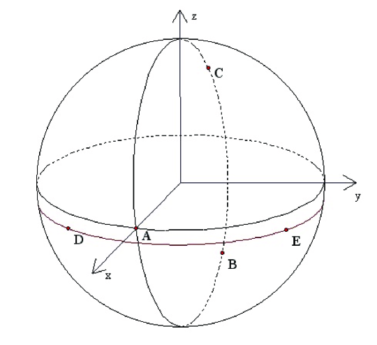
Fig. 3: The pyramid configuration

Denote the corresponding values of $(\phi_{1},\phi_{2},\theta_{2},\phi_{3},\theta_{3},\phi_{4},\theta_{4})$ by

$$\Theta_{p}=\left(-2\,\omega_{1},\dfrac{\pi}{2}-\omega_{1},\pi,\omega_{2},-\omega_{3},\omega_{2},\omega_{3}\right),$$

then the corresponding value of function $f$ is

$$\begin{split}pyfmax&=f(\Theta_{p})\\ &\approx 15.67482117.\end{split}$$ (5.2)

5.2 Domain excluded near coordinates corresponding the pyramid distribution

Similarly with the method we adopted near the bipyramid distribution, we introduce a disturbance of $\left[-\frac{\pi}{791},\frac{\pi}{791}\right]$ on coordinates corresponding the pyramid distribution, and finally obtain a rectangular domain

$$\mathcal{D}_{p}=\left(\begin{array}[]{c}\left[-{\frac{5157880419}{10000000000}},-{\frac{203137879}{400000000}}\right]\\ \vskip 6.0pt plus 2.0pt minus 2.0pt\cr\left[{\frac{1310916469}{1000000000}},{\frac{263771963}{200000000}}\right]\\ \vskip 6.0pt plus 2.0pt minus 2.0pt\cr\left[{\frac{156881049}{50000000}},{\frac{3145564327}{1000000000}}\right]\\ \vskip 6.0pt plus 2.0pt minus 2.0pt\cr\left[-{\frac{39276321}{156250000}},-{\frac{2434251099}{10000000000}}\right]\\ \vskip 6.0pt plus 2.0pt minus 2.0pt\cr\left[-{\frac{1508635943}{1000000000}},-{\frac{375173149}{250000000}}\right]\\ \vskip 6.0pt plus 2.0pt minus 2.0pt\cr\left[-{\frac{39276321}{156250000}},-{\frac{2434251099}{10000000000}}\right]\\ \vskip 6.0pt plus 2.0pt minus 2.0pt\cr\left[{\frac{375173149}{250000000}},{\frac{1508635943}{1000000000}}\right]\end{array}\right).$$ (5.3)

The interval Hessian matrix of $f$ over $\mathcal{D}_{p}$ can be calculated by interval arithmetic, i.e.,

$$\mathcal{W}=\left(W_{1},W_{2},W_{3},W_{4},W_{5},W_{6},W_{7}\right),$$ (5.4)

where $W_{i}(i=1,\ldots,7)$ are vectors

$W_{{1}}=\left(\begin{array}[]{c}\left[-{\dfrac{68555671}{80000000}},-{\dfrac{8085653887}{10000000000}}\right]\\ \vskip 6.0pt plus 2.0pt minus 2.0pt\cr\left[{\dfrac{241020403}{625000000}},{\dfrac{4060471777}{10000000000}}\right]\\ \vskip 6.0pt plus 2.0pt minus 2.0pt\cr\left[-{\dfrac{5396514777}{10000000000000}},{\dfrac{5396514777}{10000000000000}}\right]\\ \vskip 6.0pt plus 2.0pt minus 2.0pt\cr\left[-{\dfrac{665453073}{1000000000}},-{\dfrac{3261193771}{5000000000}}\right]\\ \vskip 6.0pt plus 2.0pt minus 2.0pt\cr\left[{\dfrac{323160259}{1250000000}},{\dfrac{2727361243}{10000000000}}\right]\\ \vskip 6.0pt plus 2.0pt minus 2.0pt\cr\left[-{\dfrac{6654530721}{10000000000}},-{\dfrac{6522387553}{10000000000}}\right]\\ \vskip 6.0pt plus 2.0pt minus 2.0pt\cr\left[-{\dfrac{545472247}{2000000000}},-{\dfrac{16158013}{62500000}}\right]\end{array}\right),W_{{2}}=\left(\begin{array}[]{c}\left[{\dfrac{241020403}{625000000}},{\dfrac{4060471777}{10000000000}}\right]\\ \vskip 6.0pt plus 2.0pt minus 2.0pt\cr\left[-{\dfrac{567279649}{500000000}},-{\dfrac{544204613}{500000000}}\right]\\ \vskip 6.0pt plus 2.0pt minus 2.0pt\cr\left[-{\dfrac{609173849}{50000000000}},{\dfrac{1218347717}{100000000000}}\right]\\ \vskip 6.0pt plus 2.0pt minus 2.0pt\cr\left[-{\dfrac{68583739}{400000000}},-{\dfrac{1584190467}{10000000000}}\right]\\ \vskip 6.0pt plus 2.0pt minus 2.0pt\cr\left[-{\dfrac{1486861643}{2500000000}},-{\dfrac{5875949419}{10000000000}}\right]\\ \vskip 6.0pt plus 2.0pt minus 2.0pt\cr\left[-{\dfrac{428648367}{2500000000}},-{\dfrac{792095233}{5000000000}}\right]\\ \vskip 6.0pt plus 2.0pt minus 2.0pt\cr\left[{\dfrac{2937974709}{5000000000}},{\dfrac{5947446571}{10000000000}}\right]\end{array}\right)$
$W_{{3}}=\left(\begin{array}[]{c}\left[-{\dfrac{5396514777}{10000000000000}},{\dfrac{5396514777}{10000000000000}}\right]\\ \vskip 6.0pt plus 2.0pt minus 2.0pt\cr\left[-{\dfrac{609173849}{50000000000}},{\dfrac{1218347717}{100000000000}}\right]\\ \vskip 6.0pt plus 2.0pt minus 2.0pt\cr\left[-{\dfrac{8085854539}{100000000000}},-{\dfrac{1541389841}{25000000000}}\right]\\ \vskip 6.0pt plus 2.0pt minus 2.0pt\cr\left[-{\dfrac{9959577971}{100000000000}},-{\dfrac{9385595363}{100000000000}}\right]\\ \vskip 6.0pt plus 2.0pt minus 2.0pt\cr\left[{\dfrac{116759761}{5000000000}},{\dfrac{109700733}{4000000000}}\right]\\ \vskip 6.0pt plus 2.0pt minus 2.0pt\cr\left[{\dfrac{9385595361}{100000000000}},{\dfrac{9959577971}{100000000000}}\right]\\ \vskip 6.0pt plus 2.0pt minus 2.0pt\cr\left[{\dfrac{2335195223}{100000000000}},{\dfrac{2742518293}{100000000000}}\right]\end{array}\right),W_{{4}}=\left(\begin{array}[]{c}\left[-{\dfrac{665453073}{1000000000}},-{\dfrac{3261193771}{5000000000}}\right]\\ \vskip 6.0pt plus 2.0pt minus 2.0pt\cr\left[-{\dfrac{68583739}{400000000}},-{\dfrac{1584190467}{10000000000}}\right]\\ \vskip 6.0pt plus 2.0pt minus 2.0pt\cr\left[-{\dfrac{9959577971}{100000000000}},-{\dfrac{9385595363}{100000000000}}\right]\\ \vskip 6.0pt plus 2.0pt minus 2.0pt\cr\left[-{\dfrac{8828398133}{10000000000}},-{\dfrac{1678302277}{2000000000}}\right]\\ \vskip 6.0pt plus 2.0pt minus 2.0pt\cr\left[-{\dfrac{585736263}{5000000000}},-{\dfrac{2143830967}{25000000000}}\right]\\ \vskip 6.0pt plus 2.0pt minus 2.0pt\cr\left[-{\dfrac{4897161727}{10000000000}},-{\dfrac{4822526949}{10000000000}}\right]\\ \vskip 6.0pt plus 2.0pt minus 2.0pt\cr\left[{\dfrac{616963279}{100000000000}},{\dfrac{1002395789}{100000000000}}\right]\end{array}\right)$
$W_{{5}}=\left(\begin{array}[]{c}\left[{\dfrac{323160259}{1250000000}},{\dfrac{2727361243}{10000000000}}\right]\\ \vskip 6.0pt plus 2.0pt minus 2.0pt\cr\left[-{\dfrac{1486861643}{2500000000}},-{\dfrac{5875949419}{10000000000}}\right]\\ \vskip 6.0pt plus 2.0pt minus 2.0pt\cr\left[{\dfrac{116759761}{5000000000}},{\dfrac{109700733}{4000000000}}\right]\\ \vskip 6.0pt plus 2.0pt minus 2.0pt\cr\left[-{\dfrac{585736263}{5000000000}},-{\dfrac{2143830967}{25000000000}}\right]\\ \vskip 6.0pt plus 2.0pt minus 2.0pt\cr\left[-{\dfrac{36387877}{31250000}},-{\dfrac{225679327}{200000000}}\right]\\ \vskip 6.0pt plus 2.0pt minus 2.0pt\cr\left[-{\dfrac{1002395789}{100000000000}},-{\dfrac{616963279}{100000000000}}\right]\\ \vskip 6.0pt plus 2.0pt minus 2.0pt\cr\left[{\dfrac{4813603601}{10000000000}},{\dfrac{1215175283}{2500000000}}\right]\end{array}\right),W_{{6}}=\left(\begin{array}[]{c}\left[-{\dfrac{6654530721}{10000000000}},-{\dfrac{6522387553}{10000000000}}\right]\\ \vskip 6.0pt plus 2.0pt minus 2.0pt\cr\left[-{\dfrac{428648367}{2500000000}},-{\dfrac{792095233}{5000000000}}\right]\\ \vskip 6.0pt plus 2.0pt minus 2.0pt\cr\left[{\dfrac{9385595361}{100000000000}},{\dfrac{9959577971}{100000000000}}\right]\\ \vskip 6.0pt plus 2.0pt minus 2.0pt\cr\left[-{\dfrac{4897161727}{10000000000}},-{\dfrac{4822526949}{10000000000}}\right]\\ \vskip 6.0pt plus 2.0pt minus 2.0pt\cr\left[-{\dfrac{1002395789}{100000000000}},-{\dfrac{616963279}{100000000000}}\right]\\ \vskip 6.0pt plus 2.0pt minus 2.0pt\cr\left[-{\dfrac{8828398113}{10000000000}},-{\dfrac{4195755701}{5000000000}}\right]\\ \vskip 6.0pt plus 2.0pt minus 2.0pt\cr\left[{\dfrac{171506479}{2000000000}},{\dfrac{1171472521}{10000000000}}\right]\end{array}\right)$
$W_{{7}}=\left(\begin{array}[]{c}\left[-{\dfrac{545472247}{2000000000}},-{\dfrac{16158013}{62500000}}\right]\\ \vskip 6.0pt plus 2.0pt minus 2.0pt\cr\left[{\dfrac{2937974709}{5000000000}},{\dfrac{5947446571}{10000000000}}\right]\\ \vskip 6.0pt plus 2.0pt minus 2.0pt\cr\left[{\dfrac{2335195223}{100000000000}},{\dfrac{2742518293}{100000000000}}\right]\\ \vskip 6.0pt plus 2.0pt minus 2.0pt\cr\left[{\dfrac{616963279}{100000000000}},{\dfrac{1002395789}{100000000000}}\right]\\ \vskip 6.0pt plus 2.0pt minus 2.0pt\cr\left[{\dfrac{4813603601}{10000000000}},{\dfrac{1215175283}{2500000000}}\right]\\ \vskip 6.0pt plus 2.0pt minus 2.0pt\cr\left[{\dfrac{171506479}{2000000000}},{\dfrac{1171472521}{10000000000}}\right]\\ \vskip 6.0pt plus 2.0pt minus 2.0pt\cr\left[-{\dfrac{582206031}{500000000}},-{\dfrac{564198319}{500000000}}\right]\end{array}\right)$

Through Theorem 4.5, we can judge that $\mathcal{W}$ is nonnegative semidefinite, and when the disturbance enlarges very little, it is still true. So by Theorem 4.7, we know that values of $f$ cannot attain the maximum in $\mathcal{D}_{p}$, i.e.,

Proposition 5.1.

Maximum of function $f$ can not attain in domain $\mathcal{D}_{p}$, i.e.,

$$f(\phi_{1},\phi_{2},\theta_{2},\phi_{3},\theta_{3},\phi_{4},\theta_{4})<fmax,\quad(\phi_{1},\phi_{2},\theta_{2},\phi_{3},\theta_{3},\phi_{4},\theta_{4})\in\mathcal{D}_{p}.$$ (5.5)

6 Other domains

Now, we are to prove the following strict inequality,

$$\begin{split}&f(\phi_{1},\phi_{2},\theta_{2},\phi_{3},\theta_{3},\phi_{4},\theta_{4})<fmax,\\ &\mbox{where }(\phi_{1},\phi_{2},\theta_{2},\phi_{3},\theta_{3},\phi_{4},\theta_{4})\in(\mathcal{D}^{(1)}\cup\mathcal{D}^{(2)})\backslash(\mathcal{D}_{bp}\cup\mathcal{D}_{p}).\end{split}$$ (6.1)

Algorithms in this section are implemented by procedures in the Maple package fivepoints, for the code, see appendix.

6.1 Branch and bound strategies

We check domains over which variables take using the interval method, more precisely, we compute the interval value of the interval mapping corresponding some functions through interval arithmetic, properties of this interval may suggest that, when variables take values in this domain, function $f$ has no stationary point, or its maximum is less than the value corresponding the bipyramid configuration, or it is not necessary to consider the case for symmetries. All in all, function values in this domain cannot be greater than $fmax$ (these verification methods are implemented by procedure ischecked in the package fivepoints). The followings are methods we used to exclude domains contained in $\mathcal{D}^{(1)}$ and $\mathcal{D}^{(2)}$.

1. (by Condition 3.2) Verify that $C$ is below $E$.

2. (by Condition 3.4) Verify that 5 points are in the same half sphere.

3. (by Condition 3.1) Verify that $AB$ is not the second largest distance.

4. (by Condition 3.5) Verify that the distance between some two points is less than $\dfrac{2}{15}$.

5. Verify that the upper bound of function values are less than $fmax$ (see Eq. (2.5)).

6. (by Proposition 3.3) Verify that some partial derivative of $f$ does not change signs in this domain.

7. Compute the interval Hessian matrix corresponding this domain, and determine its negative definiteness through Theorem 4.3.

8. Compute the interval Hessian matrix corresponding this domain, and determine its negative definiteness through Theorem 4.4.

9. Compute the interval Hessian matrix corresponding this domain, and determine its nonnegative definiteness through Theorem 4.5.

10. Determine there exists no maximal point in this domain through Theorem 3.1.

Different methods should be used in different domains, for example, methods 7 and 8 should be used first near points corresponding bipyramid distribution, then others (10, 5, 6) can be used; while method 9 should be used first near points corresponding pyramid distribution, then others (10, 5, 6) can be used; and for generic domains, methods can be used in turns as 1, 2, 4, 3, 5, 10, 6.

For a domain to be verified, we choose appropriate verification methods and the verification order, if verifications are not successful, we subdivide the interval whose width is maximal into two equal intervals, and verify the two subdomains recursively. We set a positive number, if the largest interval width of a domain we get in the above process is less than this number, we stop subdividing this domain, and record it, this domain may contain distributions of points corresponding larger distance sums then the maximal distance sum conjectured. This process terminates when all domains have been verified. If all domains are verified successful, and no domain is contained in the record list, then we have proved the conjecture in fact. The complete algorithm is described below (implemented as the procedure spchecked in the package fivepoints):

Input: intervallist, methods, notcheckbipyramid, notcheckpyramid

Output: true/false

AlgoLine0.1

begin  checkbipyramid := not notcheckbipyramid; checkpyramid := not notcheckpyramid; checkmethods := methods AlgoLine0.2

if checkbipyramid then  if intervallist is contained in domain bipyramidintervallist then AlgoLine0.3

#bipyramidintervallist is the rectangular domain we excluded first near the bipyramid distribution.   add $[-1]$ to checkprocess AlgoLine0.4

#record the checking processAlgoLine0.5

return true   if some variable interval in intervallist disjoints the corresponding variable interval in bipyramidintervallist then  checkbipyramid := false     AlgoLine0.6

if checkpyramid then  if intervallist is contained in domain pyramidintervallist then AlgoLine0.7

#pyramidintervallist is the rectangular domain we excluded first near the pyramid distribution.   add $[0]$ to checkprocess; return true   if some variable interval in intervallist disjoints the corresponding variable interval in pyramidintervallist then  checkpyramid := false     AlgoLine0.8

while $methods_{i}\in methods$ do  if checking domain intervallist successfully through the method $methods_{i}$ then  add $[i]$ to checkprocess; return true     AlgoLine0.9

dim := the widest interval position in interval vector intervallistAlgoLine0.10

if the width of the dim-th interval in intervallist $<$ $\frac{1}{1000}$ then  add intervallist to notchecked AlgoLine0.11

#notchecked records domains cannot be checked successfullyAlgoLine0.12

add $[-4]$ to checkprocess; return false   add dim to checkprocessAlgoLine0.13

#dim designates the variable to be subdivided, and is to be recorded in checking processAlgoLine0.14

subintervallist := subdivide the domain intervallist in the dim-th intervalAlgoLine0.15

cur := trueAlgoLine0.16

forall $subintervallist_{i}\in subintervallist$ do  if not CheckDomain($subintervallist_{i}$, checkmethods, not checkbipyramid, not checkpyramid) then  cur := false     if cur then  add $[-2]$ to checkprocess   else  add $[-3]$ to checkprocess   AlgoLine0.17

return cur endAlgoLine0.18

Algorithm 1 CheckDomain

18

18

18

18

18

18

18

18

18

18

18

18

18

18

18

18

18

18

6.2 Verification process

In order to subdivide domains into appropriate widths, we act some experiments first, finally we subdivide domains as follows: for $\mathcal{D}^{(1)}$ and $\mathcal{D}^{(2)}$ we divide in § 2, each domain is subdivided the way that each interval of it is trisected, so we get $3^{7}=2817$ subdomains each, denote them respectively by:

$$\mathcal{D}^{(1)}_{1},\mathcal{D}^{(1)}_{2},\ldots,\mathcal{D}^{(1)}_{2187},$$

and

$$\mathcal{D}^{(2)}_{1},\mathcal{D}^{(2)}_{2},\ldots,\mathcal{D}^{(2)}_{2187}.$$

If some of these subdomains are difficult to verify successfully, we can again subdivide them the same way. Actually, the following domains need to subdivide again:

$$\begin{split}&\mathcal{D}^{(1)}_{62},\mathcal{D}^{(1)}_{158},\mathcal{D}^{(1)}_{239},\mathcal{D}^{(1)}_{863},\mathcal{D}^{(1)}_{1102},\mathcal{D}^{(1)}_{1105},\mathcal{D}^{(1)}_{1106},\mathcal{D}^{(1)}_{2114},\mathcal{D}^{(1)}_{2132},\\ &\mathcal{D}^{(1)}_{1105-1101},\mathcal{D}^{(1)}_{1106-834},\mathcal{D}^{(1)}_{1106-861},\mathcal{D}^{(1)}_{1106-1099},\mathcal{D}^{(1)}_{1106-1100},\\ &\mathcal{D}^{(1)}_{1105-1101-1100},\mathcal{D}^{(1)}_{1106-834-725},\mathcal{D}^{(1)}_{1106-834-726},\\ &\mathcal{D}^{(1)}_{1106-834-725-1752},\mathcal{D}^{(1)}_{1106-834-726-1507},\mathcal{D}^{(1)}_{1106-834-726-1750},\end{split}$$ (6.2)

where $\mathcal{D}^{(1)}_{1105-1101}$ denotes the 1101-th subdomain in all 2187 subdomains of $\mathcal{D}^{(1)}_{1105}$, other similar notations are understood the same way.

6.3 Algorithm implementations

The Maple Package fivepoints implements algorithms described in above sections. For the detailed code, see Appendix LABEL:fivepoints.

7 Conclusion

The following is verification time for various domains (may differ on different computers, it is the time used by computers with Pentium IV 3.0 GHz CPU, and 1 GB RAM):

1. Time used to verify domain $\mathcal{D}^{(1)}$: $782534.203$ seconds.

2. Time used to verify domain $\mathcal{D}^{(2)}$: $8797.600$ seconds.

3. Total time: $791331.803$ seconds.

This completes the proof of the problem of spherical distribution of 5 points.

Appendix A Maple code

A.1 Module IntervalArithmetic

X

# IntervalArithmetic: a Maple package used for interval computations.

# $revision: 1.0.3.4$

IntervalArithmetic := module()

export ulp, fulb, rfulb0, rfulb,

Evalr/add, Evalr/multiply, Evalr/power,

Evalr/sin, Evalr/cos, Evalr/tan, Evalr/cot,

Evalr/arcsin, Evalr/arccos, Evalr/arctan, Evalr/arccot,

Evalr/exp, Evalr/ln, Evalr/powexp,

Evalr/shake, Evalr,

isdef, vert, inthull, intwidth, maxwidthdim, intsbdv, sortpos, contain:

local init:

option package, load = init:

##############################################################################

# initialization

##############################################################################

# the initialization procedure

init := proc()

global type/interval, type/int_ext, type/rat_ext,

type/cons, type/consnum, type/ratpar,

type/exp_user, type/ln,

convert/ft2rat, truncatenegativepart, p1, p2:

# defining the datatype of interval

type/interval := proc( inv )

if type( inv, list( rat_ext ) ) and nops( inv ) = 2

and inv[ 1 ] <= inv[ 2 ] then

true

elif inv = [ ] then

true

else

false

fi

end:

# extended datatype of integer numbers

type/int_ext := proc( x )

evalb(  type( x, integer ) or x = -infinity or x = infinity  )

end:

# extended datatype of rational numbers

type/rat_ext := proc( x )

evalb(  type( x, rational ) or x = -infinity or x = infinity  )

end:

# datatype that containing gamma, Catalan or Pi

type/cons := proc( x )

member( x, { gamma, Catalan, Pi } )

end:

# datatype of constant numbers

type/consnum := proc( x )

local c, r:

global constants:

c := constants:

constants := gamma, Catalan, Pi, infinity:

r := type( x, constant ):

constants := c:

r

end:

# datatype of functions whose parameters are rational numbers

type/ratpar := proc( f, tp::Or( set( type ), type ) )

type( f, tp ) and type( [ op( f ) ], list( rational ) )

end:

# datatype of natural exponent

type/exp_user := proc( f )

evalb( op( 0, f ) = exp )

end:

# datatype of natural logarithm

type/ln := proc( f )

evalb( op( 0, f ) = ln )

end:

# converting from float point numbers(ranges) to rational numbers(intervals)

convert/ft2rat := proc( inv )

local t:

if type( inv, float ) then

convert( inv, rational, exact )

elif type( inv, rat_ext ) then

inv

elif type( inv, list( Or( float, rat_ext ) ) ) and nops( inv ) = 2 then

t := map( procname, inv ):

if t[ 1 ] <= t[ 2 ] then t

else [ ]

fi

elif type( inv, list ) or type( inv, Matrix ) then

map( procname, inv )

else

error "invalid argument: %1", inv

fi

end:

References

• [1] H. T. Croft, K. J. Falconer, R. K. Guy. Unsolved Problems in Geometry. Springer, Berlin, 1991.
• [2] S. Smale. Mathematical problems for the next century. Math. Intelligencer 20 (2) (1998), 7-15.
• [3] S. Smale. Mathematical Problems for the Next Centruy. In Mathematics: Frontiers and Perspectives, edited by Arnold, Atiyah, Lax, and Mazui. Providence, RI: Amer. Math. Society, (2000).
• [4] G. Pólya, G. Szegö. Über den transfiniten Durchmesser (Kapazitätskonstante) von ebenen und räumlichen Punktmengen. J. Reine Angew. Math. 165 (1931), 4-49.
• [5] G. Björck. Distributions of positive mass which maximize a certain generalized energy integral. Ark. Mat. 3 (1956), 255-269.
• [6] L. Fejes Tóth. On the sum of distances determined by a pointset. Acta Math. Acad. Sci. Hung. 7 (1956), 397-401.
• [7] E. Hille. Some geometric extremal problems. J. Austral. Math. Soc. 6 (1966), 122-128.
• [8] K. B. Stolarsky. Sums of Distances Between Points on a Sphere. Proceedings of The American Mathematical Society. Vol. 35, No. 2 (1972), 547-549.
• [9] K. B. Stolarsky. Sums of Distances Between Points on a Sphere. II. Proceedings of The American Mathematical Society. Vol. 41, No. 2 (1973), 575-582.
• [10] K. B. Stolarsky. The Sum of the Distances to Certain Pointsets on the Unit Circle. Pacific Journal of Mathematics, Vol. 59, No. 1 (1975), 241-251.
• [11] K. B. Stolarsky. The Sum of the Distances to N Points on a Sphere. Pacific Journal of Mathematics, Vol. 57, No. 2 (1975), 563-573.
• [12] K. B. Stolarsky. Spherical Distributions of N Points with Maximal Distance Sums Are Well Spaced. Proceedings of the American Mathematical Society, Vol. 48, No. 1 (1975), 203-206.
• [13] R. Alexander. On the Sum of Distances between n Points on a Sphere. Acta Mathematica Academiae Scientiarum Hungaricae, Tomus 23(3-4), (1972), 443-448.
• [14] R. Alexander. On the Sum of Distances between n Points on a Sphere II. Acta Mathematica Academiae Scientiarum Hungaricae, Tomus 23(3-4), (1977), 317-320.
• [15] R. Alexander. Generalized Sums of Distances. Pacific Journal of Mathematics, Vol. 56, No. 2 (1975), 297-304.
• [16] G. D. Chakerian, M. S. Klamkin. Inequalities for Sums of Distances. The American Mathematical Monthly, Vol. 80, No. 9 (1973), 1009-1017.
• [17] J. Berman, K. Hanes. Optimizing the Arrangment of Points on the Unit Sphere. Mathematics of Computation, Vol. 31, No. 140 (1977), 1006-1008.
• [18] G. Harman. Sums of Distances Between Points of a Sphere. Internat. J. Math. Math. Sci, Vol. 5 No. 4 (1982), 707-714.
• [19] J. Beck. Sums of Distances between Points on a Sphere - an Application of the Theory of Irregularities of Distribution to Discrete Geometry. Mathematika, 31 (1984), 33-41.
• [20] Z. Füredi. The Second and The Third Smallest Distances on the Sphere. Journal of Geometry. 46 (1993), 55-65.
• [21] Ali Katanforoush, Mehrdad Shahshahani. Distributing Points on the Sphere, I. Experimental Mathematics, Vol. 12, No. 2 (2003), 199-209.
• [22] E. B. Saff, A. B. J. Kuijlaars. Distributing Many Points on a Sphere. The Mathematical Intelligencer, Vol. 19, No. 1 (1997), 5-11.
• [23] M. Jiang. On the sum of distances along a circle. Discrete Math. 2007, doi: 10.1016/ j.disc. 2007.04.025
• [24] T. Amdeberhan. On Sum of Distances On a Sphere. http://www.math.temple.edu/~tewodros/PAMS3.PDF
• [25] V. Stahl. Interval Methods for Bounding the Range of Polynomials and Solving Systems of Nonlinear Equations. PhD thesis, University of Linz, Austria. (1995).
• [26] Jiri Rohn. Positive Definiteness and Stability of Interval Matrices. SIAM J. Matrix Anal. Appl. Vol. 15, No. 1 (1994), 175-184.
• [27] Zhicheng Shi, Weibin Gao. A Necessary and Sufficient Condition for the Positive-definiteness of Interval Symmetric Matrices. Internat. J. Control. 43 (1986), 325-328.
• [28] Gene H. Golub, Charles F. Van Loan. Matirx Computation. Third Edition, (1996), The Johns Hopkins University Press.