Vaccination against rubella: Analysis of the temporal evolution of the age-dependent force of infection and the effects of different contact patterns

Abstract

In this paper, we analyze the temporal evolution of the age-dependent force of infection and incidence of rubella, after the introduction of a very specific vaccination programme in a previously nonvaccinated population where rubella was in endemic steady state. We deduce an integral equation for the age-dependent force of infection, which depends on a number of parameters that can be estimated from the force of infection in steady state prior to the vaccination program. We present the results of our simulations, which are compared with observed data. We also examine the influence of contact patterns among members of a community on the age-dependent intensity of transmission of rubella and on the results of vaccination strategies. As an example of the theory proposed, we calculate the effects of vaccination strategies for four communities from Caieiras (Brazil), Huixquilucan (Mexico), Finland and the United Kingdom. The results for each community differ considerably according to the distinct intensity and pattern of transmission in the absence of vaccination. We conclude that this simple vaccination program is not very efficient (very slow) in the goal of eradicating the disease. This gives support to a mixed strategy, proposed by Massad et al., accepted and implemented by the government of the State of São Paulo, Brazil.

I Introduction

The control of directly transmitted, viral childhood infections, around the globe has been strongly dependent on vaccination, the most effective control tool developed so far Plotkin99 . There are several infections for which vaccines exist. These are therefore candidates for eradication. Some examples include polio, measles and rubella, just to mention a few. Vaccination strategies, however, have been each time more dependent on inferences based on quantitative models, which can, through simulation tools, yield distinct scenarios and possibilities. These simulation techniques, in turn, have been proved to be invaluable tools for helping health authorities to decide between competitive strategies of eradication or control of those infections.

In previous publications Massad1994 ; Massad1995a , we applied mathematical models to design and to evaluate the impact of vaccination against rubella in the state of São Paulo, Brazil. Rubella is a viral infection that causes a mild disease, but it is considered to be a public health problem due to the risk of fetal infection and subsequent congenital defects Massad1994 ; Azevedo94 ; Plotkin2001 . Therefore, the goal of rubella vaccination is to prevent from the congenital rubella syndrome (CRS). Plotkin Plotkin2001 argues that, due to the high prevalence of rubella in some countries, only high vaccine coverage would avoid the increase of CRS.

In this paper, we analyse the effects of different contact patterns on vaccination strategies against rubella in some communities. We investigate a plausible form for the contact rate function including some constrains it must satisfy. We concentrate on the integral equation for the age-dependent force of infection — defined as the age-dependent number of new infections per capita, per unit time —, which relates the pattern of contacts among the members of a population with the prevalence of the disease, following a methodology developed elsewhere Coutinho1993 . The basic idea is to examine the force of infection in steady state that results from a given vaccination strategy.

We also turn our attention to the dynamics of the process, following the time development of the age-dependent force of infection when a vaccination strategy is started at a certain time $t$ in a previously nonimmunized population. Some aspects of the age and time dependences in epidemic models have already been studied by some authors (e.g., Greenhalgh87 ; Inaba90 ).

This paper is organized as follows. In Sec. II, we present the formalism used. We describe in detail how the contact rate function is related to the force of infection, discuss some constrains it must satisfy, and propose a form for it. In Sec. III, we describe the fitting procedures adopted to determine the values of the parameters of the contact rate function for different communities. In Sec. IV.1, we analyse the impact of specific vaccination strategies against rubella using data from communities from Caieiras, a Brazilian small town located in the neighbourhoods of São Paulo city (Azevedo Neto et al. Azevedo94 ), Huixquilucan, Mexico (Golubjatnikov et al. Golubjatnikov71 ), Finland (Edmunds et al. Edmunds00 ) and the United Kingdom (Farrington et al. Farrington01 ). It must be noted that the results from Brazil and Mexico are from nonvaccinated communities, while the results from Finland and the United Kingdom are from nonvaccinated males in communitites that have partially vaccinated female population Farrington01 ; Ukkonen96 . The results from São Paulo will be compared with those previously reported by Massad et al. Massad1994 ; Massad1995b . This paper differs from those quoted above, in that the form of the contact rate function, representing the age related pattern of contacts, was studied more carefully. Also the relation between the vaccination rate $\nu$ and the resulting proportion of vaccinated people [see Eqs. (46)-(47)] was modified. In spite of this, as we shall see, the recommended vaccination strategy was maintained, but the calculated effects of the vaccination strategies seem now to be more realistic. In Sec. IV.2, we present simulations of the temporal evolution of the force of infection and, in Sec. IV.3, we compare our results to experimental results. Finally, in Sec. V, we summarize our results.

II Mathematical Developments

II.1 Temporal Evolution

Let us assume a $SIR$ model (Susceptible–Infected–Recovered). Let $S(a,t)da$, $I(a,t)da,$ and $R(a,t)da$ be, respectively, the number of susceptible, infected and non-susceptibles (including recovered and vaccinated) individuals with ages between $a$ and $a+da$ at time $t$. We can write

$$\frac{\partial S(a,t)}{\partial a}+\frac{\partial S(a,t)}{\partial t} = -[\lambda(a,t)+\nu(a,t)+\mu]S(a,t)$$

$$\frac{\partial I(a,t)}{\partial a}+\frac{\partial I(a,t)}{\partial t} = \lambda(a,t)S(a,t)-(\mu+\gamma)I(a,t)$$ (1)

$$\frac{\partial R(a,t)}{\partial a}+\frac{\partial R(a,t)}{\partial t} = \nu(a,t)S(a,t)+\gamma I(a,t)-\mu R(a,t)\,,$$

where $\nu(a,t)$ is the age and time-dependent rate of vaccination, $\gamma$ is the recovery rate, and $\mu$ is the mortality rate, assumed constant. This type of mortality rate (constant) is known as type-II mortality function. Another type of survival curve (type I) considers that all individuals survive to exactly a certain age, and then die. Anderson and May Anderson91 mention that, for both developed and developing countries, the observed mortality function is intermediate between type I and type II, although closer to type I for developed regions.

The definition of the force of infection, as a function of age and time, is

$$\lambda(a,t)=\int_{0}^{\infty}da^{\prime}\beta(a,a^{\prime})\frac{I(a^{\prime},t)}{N(a^{\prime},t)}\quad,$$ (2)

and $N(a,t)=S(a,t)+I(a,t)+R(a,t)$ is the total number of individuals whose ages are between $a$ and $a+da$ at time $t$. In this equation, $\beta(a,a^{\prime})$ is the so-called contact rate function. It is defined so that $\beta(a,a^{\prime})dada^{\prime}$ is the number of contacts a person with age between $a$ and $a+da$ makes with all persons with age between $a^{\prime}$ and $a^{\prime}+da^{\prime}$ per unit time. Therefore, $\beta(a,a^{\prime})$ describes the contact patterns among the members of a population.

Taking into account the three equations of system (1), we can write, for $N(a,t)$,

$$\left(\frac{\partial}{\partial a}+\frac{\partial}{\partial t}\right)N(a,t)=-\mu N(a,t)\,.$$ (3)

For simplicity, we consider that, at time $t$, the total population has size $N$. In other words, we have taken $N(a,t)=N(a)=N(0)e^{-\mu a},$ for a given $t.$ In this equilibrium situation, the mortality rate equals the natality rate, and we have $N(0)=\mu N.$

II.1.1 Integral equation for $\lambda(a,t)$

Applying the method of the characteristics, as proposed by Trucco Trucco65 (see also Kot2000 ) for solving the McKendrick-Von Foerster equation, we can solve the system of equations (1).

Let $s(a,t)$ and $i(a,t)$ be the proportions of susceptible and infected individuals, among those with age $a$ at time $t$, given by

$$s(a,t)=\frac{S(a,t)}{N(a,t)}\,,\quad i(a,t)=\frac{I(a,t)}{N(a,t)}\,.$$ (4)

With these previous definitions, the first two equations of the partial differential equations system (1) can also be written as follows:

$$\frac{\partial s(a,t)}{\partial a}+\frac{\partial s(a,t)}{\partial t} = -[\lambda(a,t)+\nu(a,t)]s(a,t)$$ (5)

$$\frac{\partial i(a,t)}{\partial a}+\frac{\partial i(a,t)}{\partial t} = \lambda(a,t)s(a,t)-\gamma i(a,t)\,.$$ (6)

The boundary conditions are such that, at age $a=0$, for $t\geq 0$, we have $s(0,t)=1$ and $i(0,t)=0$. At time $t=0$, for $a\geq 0$, we have that $s(a,0)$ and $i(a,0)$ are functions of age. In the calculations, the upper limit for the age is taken to be $L=60$ yr.

Considering the change of variables (as those proposed by Trucco Trucco65 )

$$\xi = a-t$$

$$\eta = t$$

we have

$$s(a,t)=s(\xi+\eta,\eta)=s^{\prime}(\xi,\eta)$$

and similarly for $i(a,t)$, $\lambda(a,t)$ and $\nu(a,t)$.

We also have that $(\partial/\partial a+\partial/\partial t)=\partial/\partial\eta$. Thus, taking into account the above mentioned change of variables, Eq. (5) reads

$$\frac{\partial}{\partial\eta}\ln s^{\prime}(\xi,\eta)=-[\lambda^{\prime}(\xi,\eta)+\nu^{\prime}(\xi,\eta)]\quad,$$ (7)

whose generic solution can be written as

$$\ln s^{\prime}(\xi,\eta)=-\int_{p}^{\eta}[\lambda^{\prime}(\xi,x)+\nu^{\prime}(\xi,x)]dx+f(\xi)\quad,$$ (8)

where $p$ and $f(\xi)$, parameters related to the boundary conditions, are given by

$$f(\xi) = \ln s^{\prime}(\xi,0)\,,\quad p=0$$ (9)

$$f(\xi) = \ln s^{\prime}(\xi,-\xi)\,,\quad p=-\xi\quad.$$ (10)

for $\xi>0$ and $\xi<0$, respectively.

Then, for the cases in which $\xi>0$ ($a>t$) or $\xi<0$ ($a<t)$, we have, respectively, the following solutions:

$$\xi>0:\ s^{\prime}(\xi,\eta) = s^{\prime}(\xi,0)\,e^{-\int_{0}^{\eta}[\lambda^{\prime}(\xi,x)+\nu^{\prime}(\xi,x)]\,dx}$$ (11)

$$\xi<0:\ s^{\prime}(\xi,\eta) = s^{\prime}(\xi,-\xi)\,e^{-\int_{-\xi}^{\eta}[\lambda^{\prime}(\xi,x)+\nu^{\prime}(\xi,x)]\,dx}\ \ .$$ (12)

Rewriting the equations above in terms of $a$ and $t$, we obtain

$$s(a,t) = s(a-t,0)\,\exp\Bigg{[}-\int_{0}^{t}[\lambda(a-t+x,x)$$ (13)

$$+ \nu(a-t+x,x)]\,dx\Bigg{]}$$

$$s(a,t) = s(0,t-a)\,\exp\Bigg{[}-\int_{t-a}^{t}[\lambda(a-t+x,x)$$ (14)

$$+ \nu(a-t+x,x)]\,dx\Bigg{]}=$$

$$= s(0,t-a)\,\exp\Bigg{[}-\int_{0}^{a}[\lambda(z,z-a+t)$$

$$+ \nu(z,z-a+t)]\,dz\Bigg{]}\ \ .$$

for $a>t$ and $t>a$, respectively.

Equation (6)

$$\Bigg{(}\frac{\partial}{\partial a}+\frac{\partial}{\partial t}\Bigg{)}i(a,t)+\gamma i(a,t)=\lambda(a,t)s(a,t)$$ (15)

can be rewritten, with the change of variables, as

$$\frac{\partial}{\partial\eta}i^{\prime}(\xi,\eta)+\gamma i^{\prime}(\xi,\eta)=\lambda^{\prime}(\xi,\eta)s^{\prime}(\xi,\eta)\quad,$$ (16)

whose solution is

$$i^{\prime}(\xi,\eta)=e^{-\int_{q}^{\eta}\gamma ds}\Bigg{[}\int_{q}^{\eta}dx\,\lambda^{\prime}(\xi,x)s^{\prime}(\xi,x)e^{\int_{q}^{x}\gamma ds}+g(\xi)\Bigg{]}\,,$$ (17)

where $q$ and $g(\xi)$ depend on the boundary conditions:

$$g(\xi) = i^{\prime}(\xi,0)\,,\quad q=0$$ (18)

$$g(\xi) = i^{\prime}(\xi,-\xi)\,,\quad q=-\xi\quad.$$ (19)

for $\xi>0$ and $\xi<0$, respectively.

Equation (17), in terms of $a$ and $t$, is given by

$$i(a,t) = \int_{0}^{t}dt^{\prime}\,\lambda(a-t+t^{\prime},t^{\prime})s(a-t,0)\alpha(a,t,t^{\prime})+$$ (20)

$$+ e^{-\gamma t}i(a-t,0),\quad a>t,$$

$$i(a,t) = \int_{0}^{a}da^{\prime}\,\lambda(a^{\prime},a^{\prime}-a+t)s(0,t-a)\psi(a,t,a^{\prime})+$$ (21)

$$+ e^{-\gamma a}i(0,t-a),\quad a<t,$$

where $\alpha(a,t,t^{\prime})$ and $\psi(a,t,a^{\prime})$ are

$$\alpha(a,t,t^{\prime})=e^{-\int_{0}^{t^{\prime}}[\lambda(a-t+\tau,\tau)+\nu(a-t+\tau,\tau)]d\tau}e^{\gamma(t^{\prime}-t)}\,$$ (22)

and

$$\psi(a,t,a^{\prime})=e^{-\int_{0}^{a^{\prime}}[\lambda(z,z-a+t)+\nu(z,z-a+t)]dz}e^{\gamma(a^{\prime}-a)}\,.$$ (23)

The age and time-dependent force of infection [Eq. (2)] can also be written as

$$\lambda(a,t)=\int_{0}^{\infty}da^{\prime}\beta(a,a^{\prime})i(a^{\prime},t)\quad.$$ (24)

In the calculations, as already explained, the upper limit of the above integral is taken to be $L=60$ yr. Thus, replacing solutions (20) and (21) for $i(a,t)$ in the above definition, and considering that age is in the interval $0\leq a\leq L$, the integral equation for the age and time-dependent force of infection is given by

$$\lambda(a,t) = \int_{0}^{min(t,L)}da^{\prime}\,\beta(a,a^{\prime})\int_{0}^{a^{\prime}}da^{\prime\prime}\,\lambda(a^{\prime\prime},a^{\prime\prime}-a^{\prime}+t)$$ (25)

$$\times \psi(a^{\prime},t,a^{\prime\prime})+\theta(L-t)\int_{t}^{L}da^{\prime}\,\beta(a,a^{\prime})$$

$$\times \Bigg{[}\int_{0}^{t}dt^{\prime}\,\lambda(a^{\prime}-t+t^{\prime},t^{\prime})s(a^{\prime}-t,0)\alpha(a^{\prime},t,t^{\prime})$$

$$+ e^{-\gamma t}\ i(a^{\prime}-t,0)\Bigg{]}\,\,,$$

where $\theta(L-t)$ is the Heaviside function. In the following section, we study the steady state of Eq. (25).

II.1.2 Steady state behavior

Let $S(a)da$ be the number of susceptible individuals with age between $a$ and $a+da$. The fraction of potentially infectious contacts they make with actually infectives aged between $a^{\prime}$ and $a^{\prime}+da^{\prime}$ per unit time is

$$S(a)da\beta(a,a^{\prime})da^{\prime}\frac{I(a^{\prime})}{N(a^{\prime})}\quad.$$ (26)

The total number of potentially infective contacts of susceptibles aged between $a$ and $a+da$ with infectives can be obtained by integrating Eq. (26) in $da^{\prime}.$ Then, we obtain an expression for the age-dependent force of infection similar to Eq. (24).

Equation (21) in the steady state condition gives

$$i(a) = e^{-\gamma a}\Bigg{[}\int_{o}^{a}da^{\prime}e^{\gamma a^{\prime}}\lambda(a^{\prime})s(0)$$ (27)

$$\times e^{-\int_{0}^{a^{\prime}}dz[\lambda(z)+\nu(z)]}+i(0)\Bigg{]}\,\,.$$

Substituting this expression in the definition of the age-dependent force of infection in steady state we have

$$\lambda(a) = \int_{0}^{\infty}da^{\prime}\beta(a,a^{\prime})\int_{0}^{a^{\prime}}da^{\prime\prime}e^{-\gamma(a^{\prime}-a^{\prime\prime})}\lambda(a^{\prime\prime})$$ (28)

$$\times e^{-\int_{0}^{a^{\prime\prime}}dz[\lambda(z)+\nu(z)]}\quad.$$

The integral equation (28) always has $\lambda(a)=0$ as solution. According to Lopez and Coutinho Lopez2000 , depending on the parameters of the integral equation, it may have another unique positive solution.

Equation (28) is the limit for large $t$ of Eq. (25):

$$\lambda(a)=\lim_{t\to\infty}\lambda(a,t)\,.$$

II.2 Contact Patterns

II.2.1 Symmetry in the contact pattern

As mentioned in the Introduction, one of our main difficulties is to choose a correct form for the contact function $\beta(a,a^{\prime}).$ In this section, we analyze a specific situation in which $\beta(a,a^{\prime})$ has to satisfy a symmetry relation that restricts its form: if a person $A$ has a contact with a person $B$, then $B$ had a contact with $A$. In terms of transmission dynamics, it means that the total number of contacts a group $C$ of infected individuals make with a group $D$ of susceptibles equals the number of contacts group $D$ had with group $C$. This symmetry is relevant when a direct, person-to-person contact is required for transmission. For instance, a direct contact is required for sexually transmitted diseases. It seems to be at least partially required for the transmission of directly transmitted childhood diseases such as rubella.

The number of contacts the susceptibles with age between $a$ and $a+da$ make with infectives with age between $a^{\prime}$ and $a^{\prime}+da^{\prime}$, in a time interval $\partial t$, is, as we have seen,

$$S(a)da\beta(a,a^{\prime})da^{\prime}\frac{I(a^{\prime})}{N(a^{\prime})}\partial t\quad.$$ (29)

This number must be equal to the number of contacts the infectives with age between $a^{\prime}$ and $a^{\prime}+da^{\prime}$ make with the susceptibles with age between $a$ and $a+da.$ This number is

$$I(a^{\prime})da^{\prime}\beta(a^{\prime},a)da\frac{S(a)}{N(a)}\partial t\quad.$$ (30)

Thus, we must have

$$S(a)\beta(a,a^{\prime})\frac{I(a^{\prime})}{N(a^{\prime})}=I(a^{\prime})\beta(a^{\prime},a)\frac{S(a)}{N(a)}$$ (31)

or

$$\frac{\beta(a,a^{\prime})}{N(a^{\prime})}=\frac{\beta(a^{\prime},a)}{N(a)}\quad.$$ (32)

Since $N(a)=N(0)e^{-\mu a}$, we see that Eq. (32) is satisfied if $\beta(a,a^{\prime})$ has the form

$$\beta(a,a^{\prime})=e^{\mu a}h(a,a^{\prime})\quad,$$ (33)

where $h(a,a^{\prime})$ is symmetric, that is

$$h(a,a^{\prime})=h(a^{\prime},a)\quad.$$ (34)

Equation (33) will be used in the following section to construct an analytical form for $\beta(a,a^{\prime})$.

II.2.2 A form for the contact function $\beta(a,a^{\prime})$

Let us consider that rubella is approximately transmitted by direct person-to-person contact. In this case, considering that children are stratified mainly by age in classrooms Massad1995a , it is reasonable to assume that contacts are more intense among children with the same age. It is then convenient to write $h(a,a^{\prime})$ as a product of two functions,

$$h(a,a^{\prime})=f(a,a^{\prime})g(a,a^{\prime})\quad.$$ (35)

The function $f(a,a^{\prime})$ represents the longitudinal profile of $h(a,a^{\prime})$ along the plane $a=a^{\prime}$ and $g(a,a^{\prime})$ the transversal profile related to the spread of $h(a,a^{\prime})$ to both sides of the plane $a=a^{\prime}.$

We have chosen the following positively skewed function for $f(a,a^{\prime})$

$$f(a,a^{\prime})=b_{1}(a+a^{\prime})e^{-b_{2}(a+a^{\prime})}\quad,$$ (36)

and a Gaussian-like function for $g(a,a^{\prime})$

$$g(a,a^{\prime})=e^{-(a-a^{\prime})^{2}/\sigma^{2}}\quad,$$ (37)

where $\sigma=\sigma(a,a^{\prime})$ is related to the width of the Gaussian-like distribution to the sides of $a=a^{\prime}$. Considering a linear spread

$$\sigma(a,a^{\prime})=b_{3}+b_{4}(a+a^{\prime})\quad,$$ (38)

we obtain

$$h(a,a^{\prime})=b_{1}(a+a^{\prime})e^{-b_{2}(a+a^{\prime})}e^{-(a-a^{\prime})^{2}/[b_{3}+b_{4}(a+a^{\prime})]^{2}}\quad,$$ (39)

where $b_{1}$, $b_{2}$, $b_{3}$ e $b_{4}$ are the parameters to be determined.

Thus, taking into account Eq. (33), we have, for the contact function $\beta(a,a^{\prime})$,

$$\beta(a,a^{\prime})=b_{1}(a+a^{\prime})e^{-b_{2}(a+a^{\prime})}e^{-(a-a^{\prime})^{2}/[b_{3}+b_{4}(a+a^{\prime})]^{2}}e^{\mu a}\,.$$ (40)

Other functions could be chosen for $h(a,a^{\prime})$, as those proposed in Coutinho et al. Coutinho1993 and Massad et al. Massad1995a .

II.3 The relationship between vaccination rate and vaccine coverage

For our next simulations, we need to define what we mean by vaccination routine. In a nutshell, we take

$$\nu(a,t)=\nu\theta(a-a_{0})\theta(a_{1}-a)\theta(t-t_{0})\quad,$$ (41)

which has the following interpretation: after time $t_{0}$ years, children are vaccinated at a constant rate of $\nu$ children per unit of time when their ages are between $a_{0}$ and $a_{1}$. In practice, the government usually informs through the media that mothers should take their children to health centers to receive the shots. The response of parents to the government advertisement results in a given $\nu$. Enthusiastic response results in a high $\nu$.

In steady state, Eq. (41) becomes

$$\nu(a)=\nu\theta(a-a_{0})\theta(a_{1}-a)\quad.$$ (42)

We shall now calculate the relationship between $\nu$ and resulting proportion of vaccine coverage, $p$. Let $V(a)da$ be the number of vaccinated individuals with age between $a$ and $a+da$. Let $N_{v}(a)da$ be the number of non-vaccinated persons with age between $a$ and $a+da$. We have

$$\frac{dV(a)}{da} = \nu(a)N_{v}(a)-\mu V(a)$$ (43)

$$\frac{dN_{v}(a)}{da} = -\nu(a)N_{v}(a)-\mu N_{v}(a)\quad.$$ (44)

Of course, we have $V(a)+N_{v}(a)=N(a)$.

Solving Eq. (43) using the form of $\nu(a)$ given by Eq. (42), we have

$$V(a)=\left\{\begin{array}[]{l}0\ \text{,}\\ N(0)e^{-\mu a}[1-e^{-\nu(a-a_{0})}]\ ,\\ N(0)e^{-\mu a}[1-e^{-\nu(a_{1}-a_{0})}]\ ,\end{array}\begin{array}[]{l}a<a_{0}\\ a_{0}\leq a\leq a_{1}\\ a>a_{1}\end{array}\right.\quad.$$ (45)

The proportion $p$ of vaccine coverage is defined as

$$p=\frac{V(a_{1})}{N(a_{1})}=1-e^{-\nu(a_{1}-a_{0})}\quad.$$ (46)

The inverse relation between $\nu$ and $p$ is

$$\nu=\frac{\ln(1-p)}{a_{0}-a_{1}}\quad.$$ (47)

III Fitting the Model to The Data

Data consisted in seroprevalence studies carried out in communities from Mexico, Brazil, Finland and the UK.

Let $S^{+}(a)da$ be the proportion of seropositive individuals to rubella — whose serological tests were positive, indicating that they have already been infected — with ages between $a$ and $a+da$. An estimate of the function $S^{+}(a)$ resulted from fitting the serological data to (see Ref. Farrington90 )

$$S^{+}(a)=1-\exp\left\{\frac{k_{1}}{k_{2}^{2}}\left[\left(k_{2}a+1\right)e^{-k_{2}a}-1\right]\right\}\quad,$$ (48)

where $k_{i}$ $(i=1,2)$ are fitting parameters, estimated by the maximum likelihood technique for all the communities except that from Finland, which was estimated by the least squares fitting technique. Figure 1 shows the results of the fitting functions for the four communities considered, and the fitting parameters are shown in Table 1.

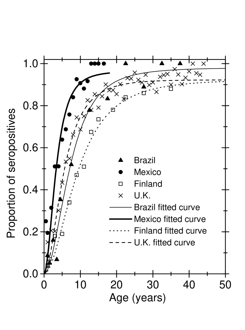
Figure 1: Seroprevalence data and corresponding fitted curves for communities from Brazil, Mexico, Finland and the UK. The data for Caieiras (Brazil), Huixquilucan (Mexico), Finland and the UK were taken, respectively, from the works of Azevedo Neto et al. Azevedo94 , Golubjatnikov et al. Golubjatnikov71 , Edmunds et al. Edmunds00 and Farrington et al. Farrington01 .

In our model, the seropositive individuals correspond to those who are either infected or nonsusceptibles (recovered and vaccinated), i.e., the proportion of seropositives, $S^{+}(a)$, is equivalent to $1-s(a)$. The force of infection in the absence of vaccination, $\lambda_{0}(a)$, was estimated from the seroprevalence data by the so-called catalytic approach (e.g., Ref. Griffiths ), according to

$$\lambda_{0}(a)=\frac{dS^{+}(a)}{da}\left(1-S^{+}(a)\right)^{-1}\quad.$$ (49)

The term catalytic arises from an analogy with chemistry. In the dynamics of infectious diseases, an infected individual would act as a catalyst, infecting susceptible individuals. Equation (49) corresponds to Eq. (5) in the steady state for the susceptible individuals, in the absence of vaccination.

Equation (49), expressed in terms of Eq. (48), results in

$$\lambda_{0}(a)=k_{1}a\exp\left[-k_{2}a\right]\quad.$$ (50)

The values of the parameters of the contact function $\beta(a,a^{\prime})$ [Eq. (40)] were calculated so that the resulting force of infection $\lambda(a)$, in the absence of vaccination, obtained by solving Eq. (28) iteratively, agreed with $\lambda_{0}(a)$ given by Eq. (50). The parameters $\gamma$ and $\mu$ were taken, respectively, to be 26.0 yr^-1, corresponding to an infectious period of 2 weeks, and 0.017yr${}^{-1},$ the inverse of a life expectancy of 60 yr. Those parameters were taken to be the same for all communities, for simplicity. The resulting parameters of the contact function $\beta(a,a^{\prime})$ for each community considered are shown in Table 1.

For Finland and the UK, we carried out simulations considering the two types of mortality functions described in Sec. II.1. As the results were very similar, we discuss only those concerning type-II mortality rate.

Table 1: Fitting parameters ($k_{1}$ and $k_{2}$) of the seroprevalence function, and the parameters of the contact function, for each community considered.

Community	$k_{1}$(yr-2)	$k_{2}$(yr-1)	$b_{1}$(yr-2)	$b_{2}$(yr-1)	$b_{3}$(yr)	$b_{4}$
Brazil	$0.0456$	$0.108$	0.658	0.0468	3.49	0.341
Mexico	$0.214$	$0.255$	3.54	0.116	1.04	0.416
Finland	0.0290	0.1068	0.587	0.0608	2.77	0.398
UK	$0.0833$	$0.1804$	1.60	0.0928	1.747	0.391

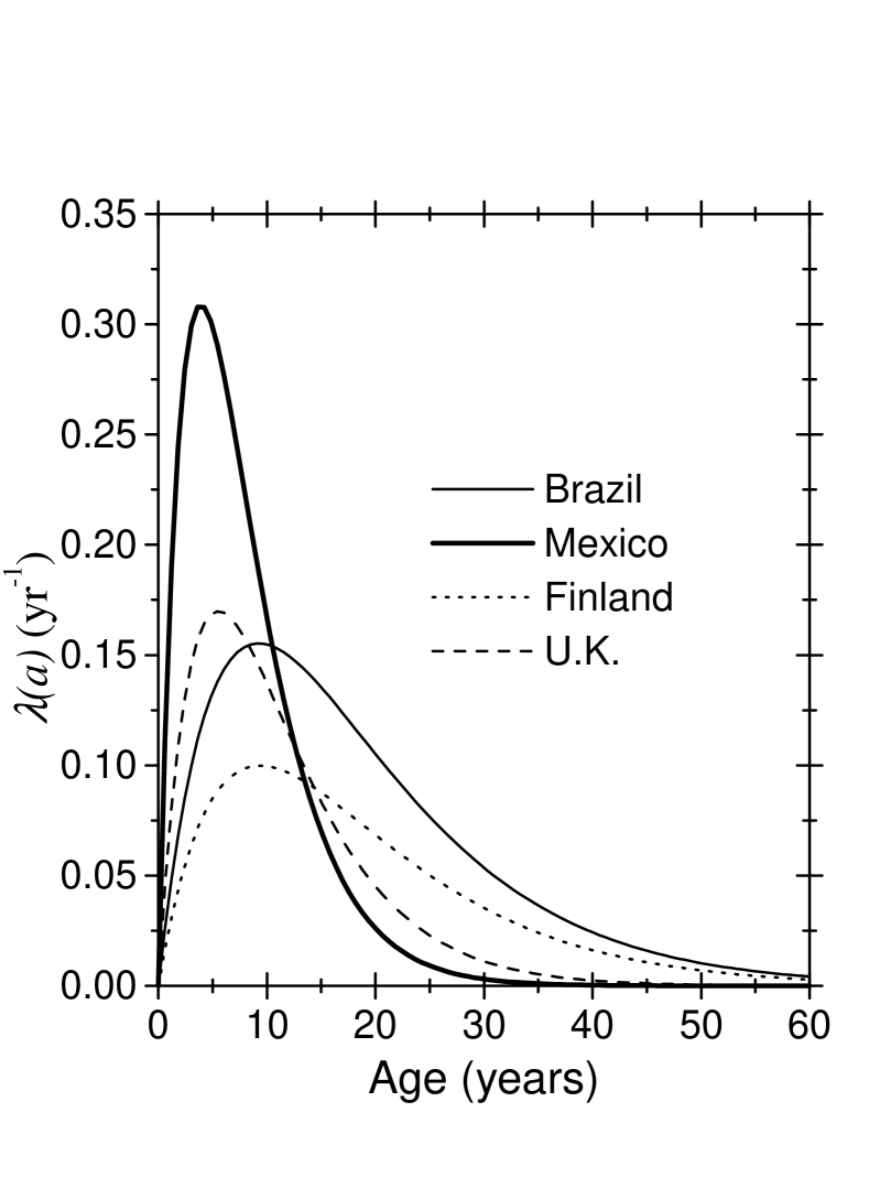
Figure 2: Force of infection for the communities studied derived from equation (50).

The forces of infection [as given by Eq. (50)] for the same communities are shown in Fig. 2. As can be noted, the curves have strikingly different shapes, reflecting distinct contact patterns. As we shall see later, this has profound impact on the calculated efficacy of different vaccination strategies.

From the force of infection, we can define the average age at which susceptibles acquire infection

$$\overline{a}=\frac{\int_{0}^{\infty}a\lambda(a)s(a)da}{\int_{0}^{\infty}\lambda(a)s(a)da}\quad.$$ (51)

We have taken the highest ages observed in the seroepidemiological studies as the upper integration limits of the integrals of Eq. (51). The calculated values for the communities studied are given in the Table 2 below.

Table 2: Average age at infection for the four communities studied.

Community	$\overline{a}$ (yr)
Caieiras, Brazil	8.45
Huixquilucan, Mexico	3.96
Finland	10.6
UK	6.64

The contact functions $\beta(a,a^{\prime})$ [Eq. (40)] of the communities considered are shown in Fig. 3 as examples of the general shape obtained. The analysis of these contact functions suggests two distinct patterns. In Mexico and in the United Kingdom, the age distribution of contacts is concentrated at lower ages. In contrast, the communities of Caieiras and Finland show a broader range of contacts, spread over all ages. In addition, it can be noted that the density of contacts estimated for the communities of Mexico and Caieiras are roughly twice as high as in the United Kingdom and Finland, respectively. This may reflect distinct social contexts between the developed and developing countries as well as the fact that data from developed communities are only for males in communities which have partially vaccinated female populations Ukkonen96 ; Farrington01 .

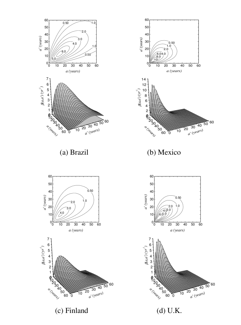
Figure 3: Calculated values of the contact functions $\beta(a,a^{\prime})$ and respective contour plots for: (a) Caieiras, Brazil; (b) Mexico; (c) Finland; and (d) the United Kingdom.

IV Simulation results

IV.1 Effects of specific vaccination strategies

We now calculate the results of specific vaccination strategies in the above mentioned communities, choosing $a_{0}=1$ year and $a_{1}=2$ years, $a_{0}=7$ years and $a_{1}=8$ years, and $a_{0}=14$ years and $a_{1}=15$ years for several values of $\nu$. For a given vaccination coverage proportion $p$, we determine $\nu$ through Eq. (47).

The simulated results of the vaccination strategies were obtained by solving Eq. (28) using the values of the parameters of $\beta(a,a^{\prime})$ obtained in Sec. III for the vaccination strategies described above.

The results for the communities of Brazil and Finland are shown, respectively, in Figures 4 and 5. The results for Mexico and UK are not shown in graphs, but we have discussed them below. Figure 4 shows the results of vaccination strategies applied to the community of São Paulo. Figures 4(a)–4(c) represent the different age intervals of vaccination. It can be noted that 75% coverage in the age interval from 1 to 2 yr almost eliminates the disease, but the peak of infection is shifted to around 17 yr, and therefore it is displaced to the right as compared with the case of no vaccination. A coverage between 79% and 80% eliminates the disease. In Fig. 4(b), it can be noted that 85% coverage in the age 7–8 yr almost eliminates the disease. In addition, the peak of infection occurs around 8 yr, and therefore it is displaced to the left as compared with the case of no vaccination. A 90% coverage in this age interval eliminates the disease. Finally, Figure 4(c) shows that vaccination in the interval from 14 to 15 yr is almost useless, since 97% coverage has very little impact in the force of infection, and it is impossible to eliminate the disease, even if a 100% coverage is used.

Figure 4: Effects of different vaccination programs calculated for Caieiras, Brazil. Children are vaccinated (a) between 1 and 2 yr , (b) between 7 and 8 yr, and (c) between 14 and 15 yr. The numbers above the dashed lines indicate the corresponding vaccine coverage and the solid lines correspond to the catalytic model. In graph (c), the dashed lines correspond, respectively, to 0.0, 0.4, 0.8 and 0.97 vaccine coverages.

Figure 5 shows the results of vaccination strategies applied to the community in Finland. Figures 5(a)–5(c) represent the different age intervals of vaccination. It can be noted that 60% coverage in the age interval 1–2 yr [Fig. 5(a)] almost eliminates the disease, and the age of the peak of infection is not affected at all. A coverage of 64% eliminates the disease. In Fig. 5(b), it can be noted that 70% coverage in the age interval 7–8 yr almost eliminates the disease, and again does not shift the age of the peak in the force of infection. Finally, Fig. 5(c) shows that vaccination in the interval from 14 to 15 yr is almost useless, since 97% coverage has very little impact on the force of infection, and it is impossible to eliminate the disease even if a 100% coverage is used.

Figure 5: Effects of different vaccination programs calculated for Finland. Children are vaccinated (a) between 1 and 2 yr, (b) between 7 and 8 yr and (c) between 14 and 15 yr. The numbers over the dashed lines indicate the corresponding vaccine coverage and the solid lines correspond to the catalytic model. In graph (c), the dashed lines correspond, respectively, to 0.0, 0.4, 0.8 and 0.97 vaccine coverages.

For the Huixquilucan community in Mexico a 74% coverage in the age interval 1–2 yr eliminates the disease. Even a 97% coverage in the age interval 7–8 yr is not able to eliminate the disease, and indeed causes very little effect on its force of infection.

For the community in the UK, a 66% coverage in the age interval 1–2 yr eliminates the disease. Even a 97% coverage in the age interval 7–8 yr is not able to eliminate the disease. However, the peak of the force of infection curve shifts leftwards to around 5 yr.

As expected, the results of vaccinating in the interval from 7 to 8 yr of age are disappointing if compared to the results of vaccinating from 1 to 2 yr of age, and vaccinating between 14 and 15 yr is almost useless.

Vaccination programmes against rubella were implemented in many countries (e.g., Refs. Edmunds00 ; Ukkonen96 ; Massad1994 ; Massad1995b ; Odette ; MMWR ). However, vaccination coverages and strategies sometimes changed from one period to another. As mentioned by Ukkonen Ukkonen96 , UK (1970) and Finland (1975) chose selective vaccination of 11- and 13-year-old girls to prevent rubella and such a strategy was not effective in eradicating the virus. These observed results agree with our simulation for vaccination from 14 to 15 yr of age. In 1998, rubella vaccine was introduced in Mexico into the childhood vaccination schedule at age 1 and 6 yr MMWR , resulting in an intense decrease in the rubella incidence, in agreement with our simulations for vaccination from 1 to 2 yr of age.

IV.2 Temporal evolution

The simulations for the temporal evolution of the force of infection were based on the numerical solutions of the integral equation for $\lambda(a,t)$, using the parameters of $\beta(a,a^{\prime})$ for the Caieiras community.

Our first simulation considered a completely susceptible population (which is not the case with Caieiras). We then assumed that, at time $t=0$, a proportion $p_{i}=10^{-5}$ of individuals with ages between 40 and 45 yr suddenly become infected. The resulting dynamics of the disease is shown in Fig. 6.

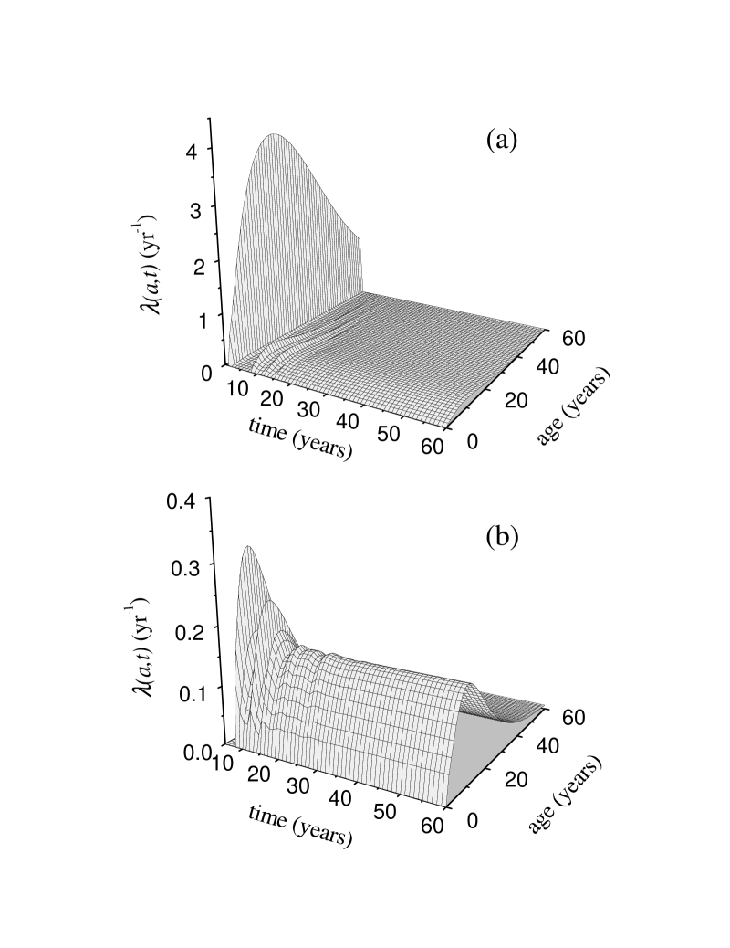
Figure 6: (a) Simulations for $\lambda(a,t)$, without vaccination, considering a completely susceptible population, at time $t=0$, except for a proportion 10^-5 of individuals with ages between 40 and 45 yr that suddenly become infected; (b) the same as (a), but with the time scale starting at $t=5$ yr, so that the initial peak is cut and the resulting steady state is observable.

It can be noted that after a few oscillations the force of infection tends to the function $\lambda_{0}(a)$. We can also see that from around 40 yr onwards the force of infection stabilizes. Figure 7 displays a profile cut at 8 yr old.

Figure 7: Profile of Fig. 6, cut at 8 yr age. The initial outbreak peak between $t=0$ and $t=3$ yr almost exhausts the susceptible fraction of the population. It takes about 3.5 years for the number of new susceptibles to accumulate in sufficient number to trigger a second outbreak which eventually stabilizes at an endemic steady state.

For our next simulation, the same conditions as the above simulation were applied, and a vaccination routine of form (41) with $a_{0}=1$ yr, $a_{1}=2$ yr, $t_{0}=40$ yr, and a vaccination coverage of 70% was added. The results for all ages are shown in Fig. 8. It can be noted that after the introduction of the vaccination, the force of infection oscillates before reaching a steady state, much lower than $\lambda_{0}(a)$. The whole process takes around 40 yr to reach the new steady state. The fact that the process takes so long to reach a steady state does not recommend this vaccination strategy for eradicating the disease.

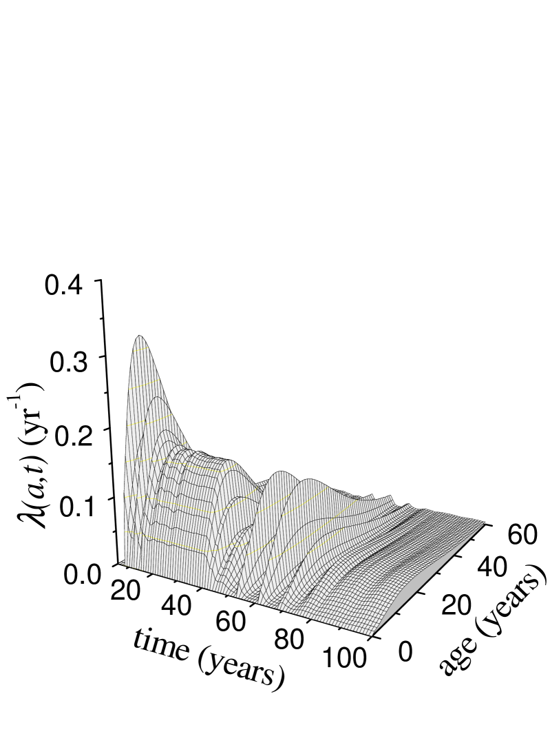
Figure 8: Simulations for $\lambda(a,t),$ with the same initial conditions considered in Fig. 6, but including a vaccination routine of form (41), with $a_{0}=1$ yr, $a_{1}=2$ yr, $t_{0}=40$ yr, and a vaccination coverage of 70%.

The next simulation uses the same vaccination scheme, but with a vaccination coverage of 80%. The results for all ages are shown in Fig. 9.

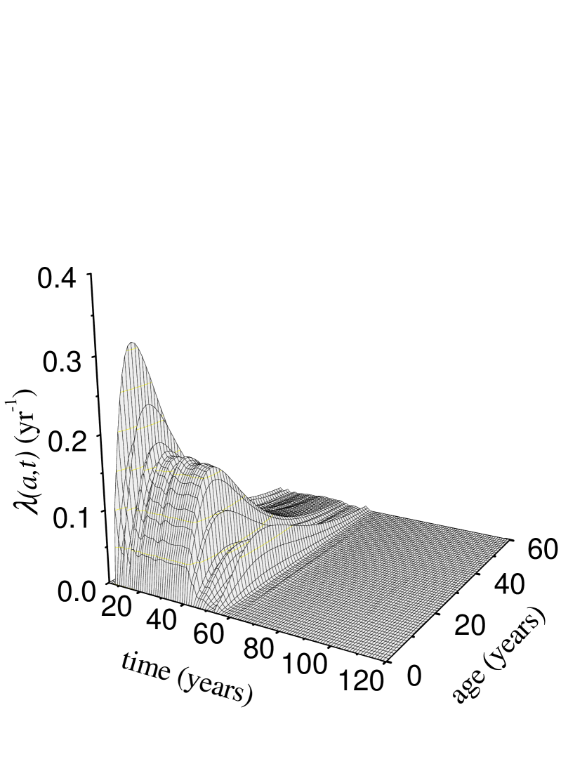
Figure 9: Vaccination scheme considered in the simulations of Fig. 8, but with a vaccination coverage of 80%.

For this coverage one can see that the disease is eradicated in approximately 20 yr. Again the fact that the process takes so long does not recommend this vaccination strategy for control.

IV.3 Comparison of specific features with real data

The strategy given by Eq. (41) was actually adopted in the United States in 1969 Plotkin99 . The results of the impact on the incidence is shown in Fig. 10 (left-hand scale) together with the results of our simulation (right-hand scale) for a $\nu$ that results in a 80% coverage. The model estimates for the number of new infections per 100 000 population were calculated according to the following equation:

$$Y(t)=\frac{1}{N}\int_{0}^{\infty}da\ \lambda(a,t)S(a,t)\quad,$$ (52)

where $\int_{0}^{\infty}da\ \lambda(a,t)S(a,t)$ is the number of new cases per unit time at time $t$. In the calculations, the upper limit of the above integral was taken to be 60 yr.

It should be noted that the incidence calculated from the seroprevalence data is two orders of magnitude larger than the incidence that results from notification. In fact, it is known that only a fraction of all infections display the clinical features of rubella disease. In addition, only a fraction of those rubella cases is officially notified. However, several qualitative features of the data are quite similar to those observed in the simulations described in the preceding section. Let us comment, in more detail, on the more significant similarities.

Figure 10: Impact on the number of reported cases (left-hand scale) of the vaccination strategy against rubella adopted in the U.S. in 1969 (data taken from CDC CDC94 ), together with the results of our simulation (right-hand scale) for a vaccination rate that results in a 80% vaccination coverage.

In 1977, that is, 8 yr after the introduction of the program, it was noted that although the program was having a major impact on rubella in children, rubella rates in those older than 15 yr were not substantially different from prevaccination rates. We shall see now that this effect is shown in our simulations.

Figure 11 represents four cuts of Fig. 8, corresponding to 70% coverage, at the ages of 8, 16, 25 and 35 yr. It can be seen that the above mentioned effect is clearly observed. The drop in the force of infection at the age of 8 yr is much larger than at 16 and 25 yr, and the effect at the age of 35 yr is almost negligible.

However, about 15 years after the introduction of the vaccine, three major outbreaks are observed in the simulations, and this may be dangerous. The pattern of several oscillations in the incidence of an infectious disease, after the introduction of vaccination, has already been observed in real data rub . If the vaccinal coverage is increased to 80%, after small outbreaks, the disease disappears, as shown in Fig. 9.

Figure 11: Profile of Fig. 8, cut at the ages of 8, 16, 25 and 35 yr.

V Summary

In this paper, we analyzed the temporal evolution of the age-dependent force of infection and incidence of rubella, after the introduction of a very specific vaccination program in a previously nonvaccinated population where rubella was in an endemic steady state. This very specific vaccination program consists in vaccinating children within a certain age range with a rate determined essentially by the public response to government advertisements.

We conclude that a simple vaccination program is not very efficient (very slow) in the goal of eradicating the disease. This gives support to a mixed strategy proposed by Massad et al. Massad1994 , accepted and implemented by the government of the State of São Paulo. This strategy recommended a mass vaccination campaign against rubella in the State of São Paulo for all children with ages between 1 and 10 yr as an initial intervention followed by a vaccination program of the form given by (41), in the routine calendar at 15 months of age. As reported in Refs. Massad1995b ; Plotkin2001 , the results were very good, and there was a considerable reduction in the number of rubella and congenital rubella syndrome cases. The incidence of rubella and CRS remained at low levels with the routine vaccination program, in agreement with our simulation results for high vaccination coverages.

We have also applied a formalism developed elsewhere Coutinho1993 to calculate the effects of vaccination routines designed to reduce or eliminate rubella.

This formalism provides an integral equation for the force of infection in a steady state given the pattern of contacts between the members of the population and the specific form of the vaccination routines.

To apply the formalism, the pattern of contacts between the members of the population, the so-called contact function $\beta(a,a^{\prime})$, has to be estimated. Some symmetries obeyed by $\beta(a,a^{\prime})$ and a general form for it were studied in Sec. II.2. In Sec. III, the force of infection in the absence of the vaccination was calculated from seroprevalence data from four communities in Brazil, Mexico, Finland and the United Kingdom. With this force of infection, in the absence of vaccination, the contact function $\beta(a,a^{\prime})$ for each community was estimated. It was noted that $\beta(a,a^{\prime})$ differed considerably between the communities studied, which is in agreement with the differences in the force of infection in the absence of vaccination.

Finally, in Sec. IV.1, the effects of several vaccination routines were calculated for the four communities studied. As a general conclusion, one can say that vaccination between 1 and 2 yr presents distinct advantages over any other strategy considered. In Caieiras, vaccination between 7 and 8 yr has the apparent advantage of shifting the average age of the first infection leftwards. However, if the coverage is above 60%, the impact of vaccinating between 1 and 2 yr on the force of infection is twice as high as vaccinating between 7 and 8 yr. This result confirms our previous analysis and recommendations of 1992 (Massad et al. Massad1994 ). In all other communities studied, vaccination between 7 and 8 yr results in very disappointing impact when compared with vaccination between 1 and 2 yr.

- (1) S. A. Plotkin and W. A. Orenstein (editors), Vaccines (Saunders, USA, 1999).
- (2) E. Massad, M. N. Burattini, R. S. Azevedo Neto, H. M. Yang, F. A. B. Coutinho, and D. M. T. Zanetta, Epidemiol. Infect. 112, 579 (1994).
- (3) E. Massad, R. S. Azevedo Neto, H. M. Yang, M. N. Burattini, and F. A. B. Coutinho, J. Biol. Syst. 3, 803 (1995).
- (4) R. S. Azevedo Neto, A. S. B. Silveira, D. J. Nokes , H. M. Yang, S. D. Passos, M. R. A. Cardoso, and E. Massad, Epidemiol. Infect. 113, 161 (1994).
- (5) S. A. Plotkin, Vaccine 19, 3311 (2001).
- (6) F. A. B. Coutinho, E. Massad, M. N. Burattini, H. M. Yang, H. M., and R. S. Azevedo Neto, IMA J. Math. Appl. Med. Biol. 10, 187 (1993).
- (7) D. Greenhalgh, IMA J. Math. Appl. Med. Biol. 4, 109 (1987).
- (8) H. Inaba, J. Math. Biol. 28, 411 (1990).
- (9) R. Golubjatnikov, W. R. Elsea, and L. Leppla, Am. J. Trop. Med. Hyg. 20, 958 (1971).
- (10) W. J. Edmunds, N. J. Gay, M. Kretzschmar, R. G. Pebody, and H. Wachmann, Epidemiol. Infect. 125, 635 (2000).
- (11) C. P. Farrington, M. N. Kanaan, and N. J. Gay, J. Roy. Stat. Soc. C (Appl. Stat.) 50, 251 (2001).
- (12) P. Ukkonen, Scand. J. Infect. Dis. 28, 31 (1996).
- (13) E. Massad, R. S. Azevedo-Neto, M. N. Burattini, D. M. T. Zanetta, F. A. B. Coutinho, H. M. Yang, J. C. Moraes, C. S. Panutti, V. A. U. F. Souza, A. S. B. Silveira, C. J. Struchiner, G. W. Oselka, M. C. C. Camargo, T. M. Omoto, and S. D. Passos, Int. J. Epidemiol. 24 (4), 842 (1995).
- (14) R. M. Anderson and R. M. May, Infectious Diseases of Humans: Dynamics and Control (Oxford University Press, Oxford, 1991).
- (15) E. Trucco, Bull. Math. Biophys. 27, 285 (1965).
- (16) M. Kot, Elements of Mathematical Ecology (Cambridge University Press, Cambridge, 2000).
- (17) L. F. Lopez and F. A. B. Coutinho, J. Math. Biol. 40, 199 (2000).
- (18) C. P. Farrington, Stat. Med. 9, 953 (1990).
- (19) D. A. Griffiths, Appl. Statist. 23, 330 (1974).
- (20) O. G. van der Heijden, M. A. E. Conyn-van Spaendock, A. D. Plantinga, and M. E. E. Kretzschmar, Epidemiol. Infect. 121, 653 (1998).
- (21) Centers for Disease Control and Prevention (CDC), MMWR 49 (46): 1048 (2000).
- (22) Centers for Disease Control and Prevention (CDC), MMWR 43 (21): 397 (1994).
- (23) E. Massad, R. S. Azevedo, M. N. Burattini, D. M. T. Zanetta, and F. A. B. Coutinho (unpublished).