A statistical-mechanical study of evolution of robustness in noisy environment

Abstract

In biological systems, expression dynamics that can provide fitted phenotype patterns with respect to a specific function have evolved through mutations. This has been observed in the evolution of proteins for realizing folding dynamics through which a target structure is shaped. We study this evolutionary process by introducing a statistical-mechanical model of interacting spins, where a configuration of spins and their interactions $\bm{J}$ represent a phenotype and genotype, respectively. The phenotype dynamics are given by a stochastic process with temperature $T_{S}$ under a Hamiltonian with $\bm{J}$. The evolution of $\bm{J}$ is also stochastic with temperature $T_{J}$ and follows mutations introduced into $\bm{J}$ and selection based on a fitness defined for a configuration of a given set of target spins. Below a certain temperature $T_{S}^{c2}$, the interactions $\bm{J}$ that achieve the target pattern evolve, whereas another phase transition is observed at $T_{S}^{c1}<T_{S}^{c2}$. At low temperatures $T_{S}<T_{S}^{c1}$, the Hamiltonian exhibits a spin-glass like phase, where the dynamics toward the target pattern require long time steps, and the fitness often decreases drastically as a result of a single mutation to $\bm{J}$. In the intermediate-temperature region, the dynamics to shape the target pattern proceed rapidly and are robust to mutations of $\bm{J}$. The interactions in this region have no frustration around the target pattern and results in funnel-type dynamics. We propose that the ubiquity of funnel-type dynamics, as observed in protein folding, is a consequence of evolution subjected to thermal noise beyond a certain level; this also leads to mutational robustness of the fitness.

I Introduction

The function of a biological unit is generally determined by a phenotype, which is the result of a dynamical process that yields a specific pattern or structure. The dynamics themselves are governed by a genetic sequence. In evolution governed by a fixed fitness condition, a phenotype that gives a higher value for the fitness function is selected. The genes that produce such a phenotype are transferred to the next generation, and thus, specific genetic sequences are selected. However, we note, that the dynamical process producing a phenotype is subject to noise. Accordingly, the genotype-phenotype mapping is generally stochastic.

For example, genetic information determines the amino acid sequence for a protein, while the tertiary structure responsible for its functions is generated only by folding dynamics. By the folding process, a structure is formed in the protein, and this structure serves as the basis for the function. The genotype-phenotype mapping is formed by this folding process, and this mapping is stochastic because of the thermal noise in the folding processSaito et al. (1997). Related folding dynamics also occur in t-RNA, where the influence of thermal noise on genotype-phenotype mapping has been intensively investigatedAncel and Fontana (2000). At a more macroscopic level, genetic information specifies a gene regulatory network, which determines the dynamics for the gene expression pattern, thus giving rise to the phenotype. This gene expression dynamics are again stochastic because the number of proteins in a cell is not necessarily very largeElowitz et al. (2002). In fact, the stochasticity for gene expression of isogenic organisms has been studied extensivelyLandry et al. (2007); Sato et al. (2003); Kaern et al. (2005). In general, a phenotype that gives rise to some particular function is generated by a dynamical process that is subject to noise. Hence, phenotypes of isogenic individual organisms are not necessarily identical, and therefore, they form a distribution.

Considering that a biological function is generally a result of such stochastic dynamics, the dynamic process that shapes the function is expected to be robust under such stochasticity; in other words, the phenotype for the function will not be sensitive to noiseAlon et al. (1999). However, such robustness is not a general property of dynamics. For example, the complex folding process of a heteropolymer from an arbitrary random sequence might not have such robustness. In this sense, the robustness could be a result of evolution. How can a dynamical process robust to noise be shaped through evolution?

In addition to being robust to noise, a biological system has to remain relatively robust to mutations in the genetic sequence that occur through evolution; the phenotype has to be rather insensitive to changes in the genetic sequence. Are these two types of robustness correlated? Does noise in the dynamic process affect the evolution of mutational robustness? Indeed, a possible relationship between robustness to noise and robustness to mutation has been discussed Ciliberti et al. (2007); Wagner (2007); J. Sun and M. W. Deem (2007); Kaneko (2006, 2007, 2008); Kaneko and Frusawa (2006), following the pioneering study by WaddingtonWaddington (1957) on the evolution-development relationship, which is referred to as canalization and genetic assimilation. However, a theoretical understanding of the evolution of robustness is still insufficient.

Consider a dynamic process for shaping a target phenotype. To have robustness to noise in such dynamics, it is ideal to adopt dynamics in which the target phenotype is reached smoothly and globally from a variety of initial configurations and is maintained thereafter. In fact, the existence of such global attraction in the protein folding process was proposed as a consistency principle by Go Go (1983) and as “funnel” landscape by Onuchic et al. Bryngelson et al. (1987); Onuchic and Wolynes (2004), while similar global attraction dynamics have been discovered recently in gene regulatory networks Li et al. (2004) and developmental dynamics Kaneko et al. (2008). In spite of the ubiquity of such funnel-like structures for phenotype dynamics, little is understood about how these structures are shaped by the evolutionary process Saito et al. (1997). We also address this question here and show that it is indeed closely related to the topic of robustness to noise.

In general, it is possible to utilize a complicated model that agrees well with biological reality in order to answer the above-mentioned questions, and this will become necessary in the future. However, at the present level of understanding, in order to understand the concepts in the evolution of robustness, we choose to investigate a rather abstract model that can be made tractable in terms of statistical physics, that is, a system consisting of $N$ Ising spins interacting globally. Each spin can take be either up or down, and each configuration of spins corresponds to a phenotype. The fitness is given by a function of the configuration of some target spins, and this fitness yields a biological function. An equilibrium spin configuration is reached by a certain Hamiltonian that is determined by the interaction between spins. This interaction is given by genes and can change by mutation. By selection according to the fitness function, a Hamiltonian that results in a higher fitness is selected. Indeed, this type of model has been adopted by Saito et al. Saito et al. (1997), who utilized it in the study of the evolution of protein folding dynamics, where the spin configuration corresponds to that of residues in a peptide chain, and the folding dynamics are given by decreasing the energy in accordance with the Hamiltonian.

Even though the spin model is abstract, it can account for the basic structures required to study the evolution of genotype and phenotype, i.e., gene $\rightarrow$ developmental dynamics subject to noise $\rightarrow$ phenotype $\rightarrow$ fitness. In comparison with the gene transcription network model utilized in the study of the evolution of robustness Ciliberti et al. (2007); Wagner (2007); Kaneko (2007, 2008), the present spin model is computationally efficient in that Monte Carlo simulations and the methods developed in statistical mechanics of spin systems can be applied to answer the above-mentioned general questions on evolution. In fact, we will analyze the evolution of robustness with respect to such a statistical-mechanical framework and define a funnel landscape in terms of frustration, as developed in spin-glass theory Nishimori (2001); M$\acute{\mbox{e}}$zard et al. (1987).

A shorter version of our results has already been published as a letter Sakata et al. (2008), in which we propose a scenario, based on our numerical simulations, that the ubiquity of funnel-type dynamics observed in biological systems is a consequence of evolutional process under noise beyond a certain level. In this paper, we further study the spin model in particular on the dependence of the result on the number of the total spins $N$ and the target spins responsible for the fitness with extensive numerical simulations. The results suggest that there exists an optimal ratio of the target to the total spins to achieve evolution of robustness over a wide range of temperature. In other words, some degree of redundant spins that do not contribute to the fitness is necessary. We have also carried out statistical-mechanical calculations of the fitness landscape, to provide an interpretation of the relation between the funnel dynamics and robustness to mutations found in our numerical simulation. These findings will stimulate further studies on the understanding on the evolution of robustness from statistical-physics viewpoints.

This paper is organized as follows. In Sec.II, we explain the model setup that captures the essential features of the evolution. In Sec.III, the numerical results for the model are presented. First, we present the dependence of energy and fitness on the temperature and selection process. Then, we show that the evolved Hamiltonians are characterized by the frustration in terms of the statistical physics of spin systems. We classify three phases on the basis of the robustness of the fitness to noise and mutation, and we show that a robust system is realized at an intermediate temperature. The system-size dependence of these results is also discussed. The origin of the robustness is studied in Sec. IV by analytically estimating the fitness landscape by using statistical mechanics. Finally, in Sec.V, the conclusions and prospects for further development are described.

II Model setup

We introduce a statistical-mechanical spin model in which the phenotype and genotype are represented by configurations of spin variables $S_{i}$ and an interaction matrix $J_{ij}$, respectively, with $i,j=1,\cdots,N$. The spins $S_{i}$ and $J_{ij}$ can take one of only two values $\pm 1$, and the interaction matrix is assumed to be symmetric, i.e., $J_{ij}=J_{ji}$. A set of configurations is denoted by $\bm{S}$ for the phenotype and by $\bm{J}$ for the genotype. The dynamics of the phenotype are given by a flip-flop update of each spin with an energy function, which is defined by the Hamiltonian for a given set of genotypes,

$$H(\bm{S}|\bm{J})=-\frac{1}{\sqrt{N}}\sum_{i<j}J_{ij}S_{i}S_{j}.$$ (1)

We adopt the Glauber dynamics as an update rule, where the $N$ spins are in contact with their own heat bath at temperature $T_{S}$. The Glauber dynamics, satisfying the detailed balance conditions, yields an equilibrium distribution for a given $\bm{J}$:

$$P(\bm{S}|\bm{J},T_{S})=\frac{e^{-\beta_{S}H(\bm{S}\mid\bm{J})}}{Z_{S}(T_{S})},$$ (2)

where $Z_{S}(T_{S})=\underset{\bm{S}}{\mbox{Tr}}e^{-\beta_{S}H(\bm{S}\mid\bm{J})}$ and $\beta_{S}=T_{S}^{-1}$. After a relaxation process, the phenotype $\bm{S}$ follows from the equilibrium distribution, and it is not determined uniquely from the genotype $\bm{J}$; rather, it is distributed, except at zero temperature. The phenotype fluctuation is computed from the Glauber dynamics, and the resulting equilibrium probability distribution. Thus, the degree of fluctuation is characterized by the temperature $T_{S}$.

Next, we introduce evolutionary dynamics for the genotype $\bm{J}$. The genotype is transmitted to the next generation with some variation, while genotypes that produce a phenotype with higher fitness are selected. The time scale for genotypic change is generally much larger than that of the phenotypic dynamics. We assume that the two time scales for the phenotypic expression dynamics and the genotypic evolutionary dynamics are separated, so that the variables $\bm{S}$ are well equilibrated within the unit time scale of the slow variable $\bm{J}$. Then, the fitness should be expressed by a function of the phenotype $\bm{S}$ that is averaged with respect to the distribution. Here, we define the fitness as

$$\Psi(\bm{J}|T_{S})=\Big{\langle}\prod_{i<j\in\bm{t}}\delta(S_{i}-S_{j})\Big{\rangle}\equiv\Big{\langle}\psi\Big{\rangle},$$ (3)

where $\langle\cdots\rangle$ denotes the expectation value with respect to the equilibrium probability distribution. The set $\bm{t}$ denotes a subset of $\bm{S}$ with size $t$ ; the members of $\bm{t}$ are termed as target spins. We refer to configurations such that all target spins are aligned in parallel as target configurations, which are assumed to give a requested appropriate function. By a gauge transformation on the target spin and the corresponding elements of $\bm{J},$ a choice of any other form of spin alignment for the fitness function, instead of the “ferromagnetic” configuration, yields the same result Nishimori (2001). The fitness can be interpreted as the average frequency of finding the target configurations in equilibrium for a given $\bm{J}$. It should be noted that in our model, only the target spins contribute explicitly to the fitness and the remaining spins have no direct influence on the fitness and the selection of genes. Hence, the spin configuration for a given fitness has redundancy.

The genotype dynamics are a result of mutations and selection, i.e., changes according to the fitness function following random flip-flops of genes. Hence, for a genetic dynamics, we once again adopt the Glauber dynamics by using the fitness instead of the Hamiltonian in the phenotype dynamics, where the genotype $\bm{J}$ is in contact with a heat bath whose temperature $T_{J}$ is different from $T_{S}$. In specific, the dynamics for the genotype are given by a stochastic Markov process with the following stationary distribution:

$$P(\bm{J}|T_{S},T_{J})=\frac{e^{\beta_{J}\Psi(\bm{J}|T_{S})}}{Z_{J}(T_{S},T_{J})},$$ (4)

where $Z_{J}(T_{S},T_{J})=\underset{\bm{J}}{\mbox{Tr}}e^{\beta_{J}\Psi(\bm{J}|T_{S})}$ and $\beta_{J}=T_{J}^{-1}$. According to the dynamics, genotypes are selected rather uniformly at high values of the temperature $T_{J}$, irrespective of the fitness, whereas at low values of $T_{J}$, the genotypes with higher fitness values are preferentially selected. In this sense, the temperature $T_{J}$ represents the selection pressure among mutated genotypes.

Figure 1: (color online) A schematic representation of our model. The plane represents the genotype space, where the circles correspond to each configuration of $\bm{J}$. Their fitness is determined through the phenotypic expression dynamics, which are given by Glauber-type dynamics. The landscape in which the height of each point corresponds to the fitness value is called a fitness landscape. At each generation of genotype evolutional dynamics, genotypes providing higher fitness values are selected under the selection pressure $T_{J}$.

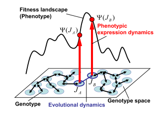
Note that the Glauber dynamics for the genotype $\bm{J}$ is applied over a much longer time scale than the dynamics for the phenotype $\bm{S}$; the genotype $\bm{J}$ changes only during the reproduction of each individual, while the spin dynamics proceed within a developmental time scale to shape the phenotype. Hence, we update $J_{ij}$ after the spins are updated a sufficient number of times for attaining the equilibrium configurations. In actual simulations, a candidate $\bm{J}^{\prime}$ for the next generation is set by some flips of a randomly chosen $J_{ij}$ from the current $\bm{J}$, while the transition probability from $\bm{J}$ to $\bm{J}^{\prime}$ is given by Metropolis rules, $\mbox{min}(1,\exp(\beta_{J}(\Psi(\bm{J})-\Psi(\bm{J}^{\prime})))$. Fig. 1 shows a schematic explanation of our model.

Our model provides two landscapes: the free energy landscape of spins and the fitness landscape of $\bm{J}$s. The free energy landscape is determined by a configuration of $\bm{J}$ and the phenotypic expression dynamics correspond to the relaxation process on the landscape. The fitness of $\bm{J}$, $\Psi(\bm{J})$, is given by the phenotypic expression dynamics on the free energy landscape of spins. We call the landscape of fitness the fitness landscape. The evolutional dynamics of $\bm{J}$ correspond to a random walk to the top of the fitness landscape; the random walk is generated by noise whose intensity is given by $T_{J}$.

A statistical-mechanical spin model similar to ours has been studied for protein evolution Saito et al. (1997), where a genetic algorithm is used for genetic dynamics. Our model, which is based on two equilibrium distributions, enables us to conduct this study by using a Markov-chain type simulation, for which a population-based simulation developed by a genetic algorithm is also available. Further, analytical tools developed in statistical mechanics are helpful for gaining a better understanding of the model.

III Results

III.1 Fitness and Energy

We have carried out MC simulations of the model discussed above and studied the dependence of the fitness and energy on $T_{S}$ and $T_{J}$. They are given by

$$\Psi(T_{S},T_{J})=[\Psi(\bm{J}|T_{S})]_{J},\ \ E(T_{S},T_{J})=[\langle H(\bm{S}|\bm{J})\rangle]_{J},$$ (5)

respectively, where $[\cdots]_{J}$ denotes the average with respect to the equilibrium probability distribution, $P(\bm{J},T_{S},T_{J})$. MC sampling with temperature $T_{S}$ under the Hamiltonian $H$ and the stochastic selection process governed by the fitness are carried out alternately. In our simulations of the spin dynamics, the exchange Monte Carlo simulation (EMC) Hukushima and Nemoto (1996) is introduced to accelerate the relaxation time to equilibrium and obtain the equilibrium spin distribution efficiently. In this section, we concentrate on the analysis of the equilibrium state. Fig. 2 (a) and (b) show the dependence of the fitness and the energy on $T_{S}$ and $T_{J}$, respectively, for $N=15$ and $t=3$. For each generation of the genotype dynamics, the fitness and energy are averaged with respect to the equilibrium distribution over 1500 MC steps after discarding the first 1500 MC steps; this number of steps is sufficient for equilibration. The data are averaged over the last 1000 generations. The dependence on the system and target size will be discussed later. For any $T_{S}$, the fitness decreases monotonically with $T_{J}$, but the rate of decrease is affected significantly by $T_{S}$. The fitness for sufficiently low $T_{S}$ remains at a high level and decreases only slightly with an increase in $T_{J}$, while for a medium value of $T_{S}$, the fitness gradually decreases to a lower level as a function of $T_{J}$, and eventually, for a sufficiently high value of $T_{S}$, it never reaches a high level. This result implies that the structure of the fitness landscape depends on $T_{S}$, the temperature at which the system has evolved.

Figure 2: (color online) The density plots of the fitness $\Psi(\bm{J})$ and the energy (both are given as Eq. (5)) are shown in (a) and (b), respectively, in the $T_{S}-T_{J}$ plane with $N=15$ and $t=3$.

The energy function, on the other hand, shows a significant dependence on $T_{S}$. While the energy is represented by a monotonically increasing function of $T_{S}$, for high $T_{J}$, it exhibits non-monotonic behavior for low $T_{J}$ and has a minimum at $T_{S}\simeq 2.0$. The configurations that include the target pattern at the energy minimum are obtained around $T_{S}\simeq 2.0$. This non-monotonicity of the energy corresponds to a negative specific heat in the sense of standard thermodynamics. This is not possible in quenched spin systems with fixed $\bm{J}$. However, the interactions $\bm{J}$ depend on the temperature $T_{S}$ and $T_{J}$. It would be convenient to obtain an explicit formula for the derivative of the energy with respect to $T_{S}$:

$$\frac{dE(T_{S},n)}{dT_{S}}=\beta_{S}^{2}\Big{\{}[\sigma_{E}^{2}]_{J}+\beta_{J}\mbox{Cov}_{\bm{J}}\Big{(}\langle H\rangle,\mbox{Cov}_{\bm{S}}(\psi,H)\Big{)}\Big{\}},$$ (6)

where $\mbox{Cov}_{\bm{J}}(A,B)=[AB]_{J}-[A]_{J}[B]_{J}$, $\mbox{Cov}_{\bm{S}}(A,B)=\langle AB\rangle-\langle A\rangle\langle B\rangle$ and $\sigma_{E}^{2}=\langle H^{2}\rangle-\langle H\rangle^{2}$. The first term of Eq. (6) is the usual specific heat of the random system and it must be positive, and $T_{S}$-dependence of $\bm{J}$ comes from the second term, which can be negative.

The configurations of $\bm{J}$ giving rise to the highest fitness value generally have a huge redundancy. Using a fluctuation induced by $T_{S}$, a specific subset of the configurations of $\bm{J}$ with lower energy is selected among the redundant configurations at around $T_{S}\simeq 2.0$.

III.2 Frustration

Figure 3: (color online) Definition of frustration in terms of the parameters $\Phi_{1},\Phi_{2},$ and $\Phi_{3}$ for the case with three target spins ($t=3$); $S_{i}\ (i=1,2,3)$ are target spins and the remaining spins are non-targets. The bold lines depict the interactions between target spins ($\in\bm{J}_{tt}$), the dashed lines depict those between target and non-target spins ($\in\bm{J}_{to}$), and the dotted lines depict those between non-target spins ($\in\bm{J}_{oo}$); (a) a triangle consists of three $\bm{J}_{tt}$ interactions; (b) a triangle consists of one $\bm{J}_{tt}$ interaction and two $\bm{J}_{to}$ interactions which are connected to the same non-target spin; (c) a hexahedron that consists of all types of interactions. By summing up the target spins, it is represented as a triangle with a renormalized interaction.

In the medium-temperature range, both a lower energy and a higher fitness are achieved. What is the structure in $\bm{J}$ configurations that helps to achieve this? The statistical physics of spin systems tells us that a decrease in energy implies a decrease in the frustration in spin configurations. By the definition of the Hamiltonian Eq. (1), the possible minimum energy is $-C_{2}^{N}/\sqrt{N}$, where $C_{2}^{N}$ is the number of the spin pairs. However, if the interaction among the three spins satisfies $J_{ij}J_{jk}J_{ki}<0$, the energy per spin cannot be minimized to the minimum value $-C_{2}^{N}/\sqrt{N}$. Such interactions are said to have frustrationNishimori (2001); M$\acute{\mbox{e}}$zard et al. (1987). Meanwhile, all the interactions satisfying $J_{ij}J_{jk}J_{ki}>0$ do not have frustration, and the energy of the spin states attains the minimum value. However, the energetically favorable spin configuration cannot be uniquely determined only by the condition $J_{ij}J_{jk}J_{ki}>0$. The spin configurations that have low energy should be the target configurations when both the decrease in energy and the increase in fitness are simultaneously achieved. In our case, the target spins play a distinct role, and therefore, we need to quantify the frustration while distinguishing between target and non-target spins; this is in contrast to the standard spin-glass study.

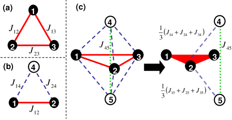
The interactions are divided into three categories: those between target spins, $\bm{J}_{tt}\ (\{J_{ij}\mid i,j\in\bm{t}\})$, those between target and non-target spins, $\bm{J}_{to}\ (\{J_{ij}\mid i\in\bm{t},j\in/\ \bm{t}\})$, and those between non-target spins, $\bm{J}_{oo}\ (\{J_{ij}\mid i,j\in/\ \bm{t}\})$. It can be assumed that the frustration of all categories decreases at intermediate $T_{S}$. To confirm this, we should define the conditional frustration for each category of spins. Fig. 3(a) shows the minimal configuration consisting of the interactions in $\bm{J}_{tt},$ (b) shows that consisting of the interactions in $\bm{J}_{tt}$ and $\bm{J}_{to}$, and (c) shows that consisting of the interactions in $\bm{J}_{to}$ and $\bm{J}_{oo}$.

Figure 4: (color online) Density plot of local frustrations: (a) $\Phi_{1}$, (b) $\Phi_{2},$ and (c) $\Phi_{3}$ in the $T_{S}-T_{J}$ plane. The data are computed by averaging over 150 genotypes $\bm{J}$ evolved at given temperatures $T_{S}$ and $T_{J}$ with $N=15$ and $t=3$.

We first define $\Phi_{1}$ as the frequency of positive coupling among target spins, i.e.,

$$\Phi_{1}(T_{S},T_{J})=\frac{2}{t(t-1)}\Big{[}\sum_{i<j\in\bm{t}}J_{ij}\Big{]}_{J}.$$ (7)

The target configurations are energetically preferred under ferromagnetic coupling, i.e., $\Phi_{1}=1$, for which no frustration exists among the target spins (Fig. 3(a)).

Second, we define $\Phi_{2}$ as

$$\Phi_{2}(T_{S},T_{J})=\frac{2}{t(t-1)(N-t)}\Big{[}\sum_{i<j\in\bm{t}}\sum_{k\in/\bm{t}}J_{ik}J_{jk}\Big{]}_{J},$$ (8)

where $t(t-1)(N-t)/2$ is the total number of possible spins: two target spins and one non-target spin. Here, $\Phi_{2}=1$ implies that no frustration exists in the interactions between target and non-target spins, and thus, the target configuration is at an energy minimum even when these interactions are included (Fig. 3(b)).

Lastly, as a measure of the frustration among non-target spins, $\Phi_{3}$ is defined as

$$\Phi_{3}(T_{S},T_{J})=\frac{1}{C_{2}^{N-t}}\Big{[}\sum_{k<l\in/\bm{t}}\Big{(}\frac{1}{t}\sum_{i\in\bm{t}}J_{ik}\Big{)}J_{kl}\Big{(}\frac{1}{t}\sum_{j\in\bm{t}}J_{jl}\Big{)}\Big{]}_{J},$$ (9)

where $C_{2}^{N-t}$ is the total number of possible pairs of non-target spins. Fig. 3(c) helps to comprehend the definition of $\Phi_{3}$. Each non-target spin interacts with all the target spins, and it has $t$ interactions that are categorized into $\bm{J}_{to}$, e.g., $J_{14},J_{24}$ and $J_{34}$. By summing up all the interactions, the frustration is computed as $\frac{1}{9}(\sum_{i=1}^{3}J_{i4})J_{45}(\sum_{j=1}^{3}J_{5j})$. By considering all the possible non-target spins instead of sites 4 and 5, $\Phi_{3}$ is defined as Eq. (9). If $\Phi_{3}$ is equal to 1, the frustration is not introduced by the interactions between non-target spins; in other words, there is no frustration globally. Hence, the system with $\Phi_{1}=\Phi_{2}=\Phi_{3}=1$ is in the Mattis state Mattis (1976), which can be transformed to ferromagnetic interaction by a gauge transformation.

For the interaction $\bm{J}$, with evolution under an environment with temperature $T_{S}$, we have computed $\Phi_{1},\Phi_{2}$, and $\Phi_{3}$ by performing MC simulations. In Fig. 4, we present contour maps of (a) $\Phi_{1}(T_{S},T_{J})$, (b) $\Phi_{2}(T_{S},T_{J})$, and (c) $\Phi_{3}(T_{S},T_{J})$ in the $T_{S}-T_{J}$ plane. At sufficiently low $T_{J}$, the frustration parameters attain the maximum value 1 at the intermediate $T_{S}$, where the frustrations are extensively eliminated, while they remain finite at low $T_{S}$ and high $T_{S}$. We define the intermediate temperature region as $T_{S}^{c1}<T_{S}<T_{S}^{c2},$ where the frustration parameter $\Phi_{2}$ equals 1. These temperatures depend on $T_{J}$, and we express them as $T_{S}^{c1}(T_{J})$ and $T_{S}^{c2}(T_{J})$. We see that for low $T_{J}$ ($\hskip 3.00003pt\raisebox{1.72218pt}{$<$}\raisebox{-3.01385pt}{$\sim$}\hskip 3.00003pt0.05$), the phase diagram is split into three phases. The first one is frustrated and adapted phases for $T_{S}<T_{S}^{c1}(T_{J})$. For $T_{S}<T_{S}^{c1}(T_{J})$, all $\Phi_{i}~{}(i=1,2,3)$ are less than unity, and hence, the frustration remains for target and non-target spins.

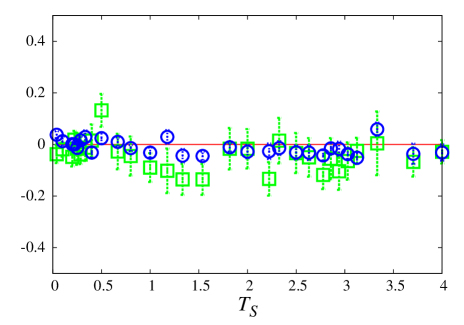
For $T_{S}\geq T_{S}^{c1}(T_{J})$, $\Phi_{1}$ equals 1, so that a target configuration is embedded as an energetically favorable state (Fig. 4(a)). For a finite system with finite $T_{J}$, $\Phi_{j}$ cannot be exactly 1. However, as long as $T_{J}$ is low, the deviation of $\Phi_{j}$ from 1 at the intermediate temperature is negligible. In contrast to $\Phi_{1}$, the sum of the $J_{ij}$ in $\bm{J}_{to}$ and $\bm{J}_{oo}$ fluctuates around $0$ at any $T_{S}$. Fig. 5 shows the averages $\overline{\bm{J}_{to}}=[\sum_{i\in\bm{t},j\in\bm{o}}J_{ij}]_{J}$ and $\overline{\bm{J}_{oo}}=[\sum_{i\in\bm{o},j\in\bm{o}}J_{ij}]_{J}$ of the summation of $J_{ij}$ in $\bm{J}_{to}$ and $\bm{J}_{oo}$, respectively, at a low $T_{J}$ ($0.5\times 10^{-3}$). As shown in Fig. 5, $\overline{\bm{J}_{to}}$ and $\overline{\bm{J}_{oo}}$ do not deviate from 0 at any $T_{S}$. This implies that no specific patterns are embedded in the spin configuration apart from the target spins.

For $T_{S}^{c1}(T_{J})\leq T_{S}\leq T_{S}^{c2}(T_{J})$, $\Phi_{2}$ is also equal to 1, implying that the frustration among spins is not introduced via interactions with a non-target spin (Fig. 4(b)). In this temperature range, $\Phi_{3}$ is not always equal to 1, except for $T_{S}\sim 2.0$, where the Mattis state arises (Fig. 4(c)). When $\Phi_{2}=1$ and $\Phi_{3}\neq 1$, the frustration is not completely eliminated from the non-target spin interactions $\bm{J}_{oo}$; this is in contrast to the Mattis state. We call such a $\bm{J}$ configuration “local Mattis state,” and it is characterized by $\Phi_{1}=\Phi_{2}=1$ but $\Phi_{3}\neq 1$. This implies that the interactions $\bm{J}$ have no frustration around the target spins, but there is some frustration between non-target spin interactions. The interactions $\bm{J}$ required to form such a local Mattis state are obtained as a consequence of the evolution around $T_{S}^{c1}(T_{J})\leq T_{S}\leq T_{S}^{c2}(T_{J})$ for low $T_{J}$, where both the fitted target configuration and lower energy are achieved. The $T_{S}$ range in which the local Mattis state is stabilized becomes narrower with an increase in $T_{J}$. The phase diagram of the model is shown in Fig. 6.

Figure 5: (color online) $T_{S}$-dependence of the averages $\overline{\bm{J}_{to}}$ $(\square)$ and $\overline{\bm{J}_{oo}}$ $(\bigcirc)$ for a fixed $T_{J}=0.5\times 10^{-3}$.

Figure 6: Phase diagram of the evolved $\bm{J}$s at $N=15$ and $t=3$. Three types of evolved $\bm{J}$ are defined on the basis of the value of the fitness and $\Phi_{2}$. Their properties are summarized below in Table 1.

For $T_{S}>T_{S}^{c2}(T_{S})$, the frustration parameter $\Phi_{2}$ is less than 1, and consequently, the frustration remains, and the fitness $\Psi$ starts to decrease and the energy increases. Thus, neither adaptation nor energy minimization is achieved. The parameters $\Phi_{i}$s should converge to 0 as $T_{S}\to\infty$, because for random $\bm{J}$, the numbers of frustrated and non-frustrated loops are equal. In fact, at $T_{S}\sim 5.0$, $\Phi_{1}$ also starts to decrease.

III.3 Relaxation dynamics

Thus far, we have computed the fitness in the equilibrium state by using EMC for accelerating the relaxation dynamics of spins. Under standard Glauber dynamics, the process may require much longer time steps. Here, we discuss the relaxation dynamics of spins for adapted interactions $\bm{J}$ that are obtained from evolution under the condition of given $T_{S}$ and $T_{J}$. The target magnetization $m_{t}=|\frac{1}{t}\sum_{i\in\bm{t}}S_{i}|$ is computed as a function of time. Note that we do not use EMC here; rather, we adopt standard MC to directly observe the energy landscape of $\bm{J}$ adapted through evolution. We calculate the average of $m_{t}$ over $\bm{J}$ drawn from an equilibrium distribution $P(\bm{J},T_{S},T_{J})$ at $T_{S}$ and $T_{J}$. Fig. 7 (a) shows the relaxation dynamics of $\langle\langle m_{t}\rangle\rangle$ for $T_{S}=10^{-3}(\leq T_{S}^{c1})$ and $T_{S}=2.0(T_{S}^{c1}\leq T_{S}\leq T_{S}^{c2})$, where $\langle\langle\cdots\rangle\rangle$ denotes the average over the initial conditions randomly chosen and over interactions $\bm{J},$ according to $P(\bm{J},T_{S},T_{J})$. In the simulation, we choose a sufficient low $T_{J}(=10^{-3})$ so that the obtained interactions have high fitness values. A common working temperature $T_{S}^{\prime}(=10^{-5})$ for relaxation is also chosen to be very low in order to examine the $T_{S}$-dependence of the adapted interactions $\bm{J}$ at $T_{S}$ and $T_{J}$. By performing this simulation, the landscape properties of the typical $\bm{J}$ adapted at $T_{S}$ are clearly determined from a dynamical viewpoint. As shown in Fig. 7, the relaxation process of $\langle\langle m_{t}\rangle\rangle$ for low $T_{S}$ is much slower even when the working temperatures $T_{S}^{\prime}$ are the same. Furthermore, the relaxation process converges to a value $m_{t}^{\ast}$ that is less than 1 and remains at that value for a long time. The deviation of $\langle\langle m_{t}\rangle\rangle$ from 1 gives the fraction of the initial conditions that fails to reach the target within this time span, because each $m_{t}$ for $t=3$ is either 1 or $1/3$ depending on whether the target configuration is reached. Indeed, the relaxation dynamics are strongly dependent on the initial conditions. For some initial conditions, the spins are trapped at a local minimum, and as a result, the target configuration is not realized over a long time span. After a much longer time span, $\langle\langle m_{t}\rangle\rangle$ approaches 1, the equilibrium value, when the spins are updated under the temperature $T_{S}$, i.e., the temperature adopted for evolution. Such dependence on initial conditions is not observed for $\langle\langle m_{t}\rangle\rangle$ when $T_{S}>T_{S}^{c1}$, where $\langle\langle m_{t}\rangle\rangle$ approaches 1 rather quickly.

Figure 7: (color online) (a) Relaxation dynamics of the averaged magnetization of target spins, $\langle\langle m_{t}\rangle\rangle,$ averaged over the adapted interactions $\bm{J}$ for $T_{S}=10^{-3}$ (solid curve) and $T_{S}=2.0$ (dashed curve). The magnetization $\langle\langle m_{t}\rangle\rangle$ is evaluated by calculating the average over 30 initial conditions for each $\bm{J}$ and 1000 different samples of $\bm{J}$ that are drawn from $P(\bm{J},T_{S},T_{J}=10^{-3})$.
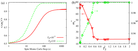
(b)The $T_{S}$-dependence of the estimated convergent value of $\langle\langle m_{t}\rangle\rangle$, $m_{t}^{\ast}$ on the right axis and the relaxation time $\tau$ on the left. The relaxation time is estimated from the time constant of an exponential decay of $\langle\langle m_{t}\rangle\rangle$.

From an estimate of the convergent value of the target magnetization, $m_{t}^{\ast},$ within a given time scale, we obtain the relaxation time $\tau$ by fitting the estimates to the function $\langle\langle m_{t}\rangle\rangle(s)=m_{t}^{\ast}+c\exp(-s/\tau)$, where $s$ is the Monte Carlo step of the spin dynamics. The parameters $m_{t}^{\ast}$ and $\tau$ are plotted against $T_{S}$ in Fig. 7(b), which shows that $\tau$ starts to increase and $m_{t}^{\ast}$ decreases from 1 as $T_{S}$ decreases below $T_{S}^{c1}$. These results imply that the interactions $\bm{J}$ whose energy landscapes are rugged, similar to the energy landscape of a spin-glass phase, are dominant for $T_{S}\leq T_{S}^{c1}$, whereas those with a smooth landscape around the target are dominant for $T_{S}^{c1}\leq T_{S}\leq T_{S}^{c2}$. The latter can be interpreted as a type of funnel landscape. Our result supports the occurrence of transitions from the spin-glass phase to the funnel phase at $T_{S}^{c1}$caused by thermal fluctuation. Note that the evolutional formation of funnel from rugged landscapes was also observed by Saito et al. in the evolution simulations of spin systems for protein folding Saito et al. (1997).

III.4 Robustness to mutation

We now examine the mutational robustness of the evolved genotypes in detail. The robustness to mutations corresponds to the stability of the fitness of $\bm{J}$ with respect to changes in the $\bm{J}$ configuration. From the genotypes $\bm{J}$ that are generated by $P(\bm{J}|T_{S},T_{J})$, mutations are imposed by flipping the sign of a certain fraction of randomly chosen matrix elements in $\bm{J}$. The value of the fraction corresponds to the mutation rate $\mu$. We evaluate the fitness of the mutated $\bm{J}^{\prime}(\bm{J},\mu)$ at $T_{S}^{\prime}$, i.e.,

$$[\Psi(\bm{J}^{\prime} (\bm{J},\mu)|T_{S}^{\prime})]_{J(T_{S},T_{J})}$$

$$=\underset{\bm{J}}{\mbox{Tr}}P(\bm{J}|T_{S},T_{J})\frac{\underset{\bm{S}}{\mbox{Tr}}\psi e^{-\beta_{S}^{\prime}H(\bm{S}|\bm{J}^{\prime}(\bm{J},\mu))}}{Z(T_{S}^{\prime},\bm{J}^{\prime}(\bm{J},\mu))},$$ (10)

where $\beta_{S}^{\prime}=1/T_{S}^{\prime}$ and $Z(T_{S}^{\prime},\bm{J}^{\prime})=\underset{\bm{S}}{\mbox{Tr}}e^{(-\beta_{S}^{\prime}H(\bm{S}|\bm{J}^{\prime}))}$. The bracket $[\cdots]_{J(T_{S},T_{J})}$ is almost identical to that denoted by $[\cdots]_{J}$ defined above; however, the additional subscript $(T_{S},T_{J})$ indicates the temperatures at which the genotype $\bm{J}$ evolves. If $\mu=0$ and $T_{S}^{\prime}=T_{S}$, $[\cdots]_{J(T_{S},T_{J})}$ is equal to the usual fitness defined in Eq. (5); $[\Psi(\bm{J}^{\prime}(\mu=0)|T_{S}^{\prime}=T_{S})]_{J(T_{S},T_{J})}=\Psi(T_{S},T_{J})$. In order to distinguish the mutational robustness from thermal noise, we set $T_{J}=0.5\times 10^{-3}$ to ensure that the fitness value with $\mu=0$ is 1 and the working temperature is $T_{S}^{\prime}=10^{-5}$. The fitness averaged over 150 samples of mutated $\bm{J}^{\prime}$ is plotted against the mutation rate $\mu$ in Fig. 4 in Sakata et al. (2008) for $T_{S}=10^{-4}$ and $T_{S}=2.0$. For low $T_{S}$, the fitness of mutated $\bm{J}$ exhibits a rapid decrease with an increase in the mutation rate, but when $T_{S}$ is between $T_{S}^{c1}$ and $T_{S}^{c2}$, the fitness does not decrease until the mutation rate reaches a specific value. We define $\mu_{c}(T_{S})$ as a threshold mutation rate beyond which the fitness $[\Psi(\bm{J}^{\prime}(\bm{J},\mu)|T_{S}^{\prime})]_{J(T_{S},T_{J})}$ drops below 1. The value $\mu_{c}$ has a plateau at $T_{S}^{c1}\leq T_{S}\leq T_{S}^{c2}$. The range of temperatures that result in mutational robustness as evolution proceeds agrees with the range giving rise to the local Mattis state, where $\Phi_{2}$ is unity. In other words, mutational robustness is realized for a set of genotypes with no frustration around the target spins. The evolution to a mutationally robust genotype $\bm{J}$ is possible only when the phenotype dynamics are subjected to noise in the range $T_{S}^{c1}\leq T_{S}\leq T_{S}^{c2}$.

Phase	Adaptation	Frustration	Landscape	Robustness
SG	Adapted	Frustrated	Rugged	Not robust
LMS	Adapted	Not frustrated	Funnel	Robust
PM	Not adapted	Frustrated	Rugged	Not robust

Table 1: Three types of $\bm{J}$—spin-glass (SG), local Mattis state (LMS), and paramagnetic state (PM)—are defined by the value of the local frustration parameter $\Phi_{2}$ (Fig. 6). The adaptation and frustration of $\bm{J}$s have been studied in the previous sections, and their landscape and robustness at a working temperature $T_{S}^{\prime}$ have been studied in this section. We have adopted a very low temperature $T_{S}^{\prime}$ to reveal the energy and fitness landscape given by the interaction matrix $\bm{J}$ evolved at each temperature $T_{S}$. The $\bm{J}$s evolved at $T_{S}<T_{S}^{c1}$ (these $\bm{J}$s belong to the SG phase) have high fitness values and frustrations. Their adaptation is not robust to noise and mutation because of their rugged landscapes. The $\bm{J}$s evolved at $T_{S}^{c1}<T_{S}<T_{S}^{c2}$, (these $\bm{J}$s belong to the LMS phase) have high fitness values and less frustrations. They are robust to noise and mutation, and their landscapes give funnel-type dynamics for spins. The fitness values of the $\bm{J}$s evolved at $T_{S}>T_{S}^{c2}$ (these $\bm{J}$s belong to the PM phase) cannot be high, and the $\bm{J}$s have frustrations.

To summarize, there are three phases, local Mattis, spin glass and paramagnetic disorder ones, for the evolved $\bm{J}$, as shown in Fig. 6. Each phase defined by the frustration parameter $\Phi_{2}$ has a distinct characteristic feature in relaxation dynamics and some robustness, that are summarized in Table 1.

III.5 Size dependence and the existence of an optimal target size to obtain LMS

Figure 8: (color online) The $T_{S}$-dependence of (a) the fitness, (b) the energy, and (c) the frustration parameter $\Phi_{2}$ at $N=15,~{}t=3$, $N=20,~{}t=4$ and $N=30,t=6$. The temperature $T_{J}$ is fixed at $0.5\times 10^{-3}$. The inset of each figure shows the dependence of each quantity on the temperature rescaled by $\sqrt{N}$. The vertical axis of the inset of (b) is also rescaled by $\sqrt{N}$.

Figure 9: (color online) The $T_{S}$-dependence of (a) the fitness, (b) the energy, and (c) $\Phi_{2}$ at $N=30$ and $t=3,6,9,12$, and $15$. The temperature $T_{J}$ is fixed at $0.5\times 10^{-3}$. The convergence value of the fitness (a) at $T_{S}\to\infty$ is $2^{-t+1}$.

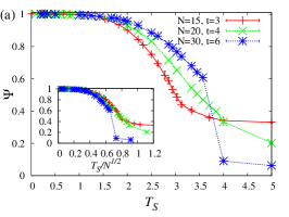
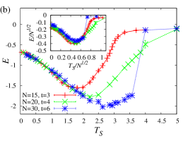
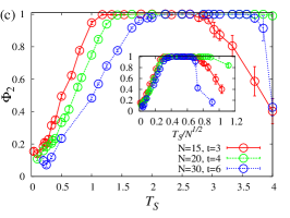
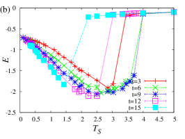
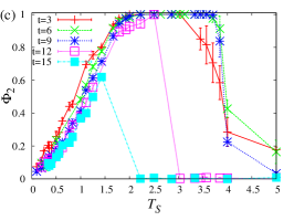
To check the generality of the transition to the local Mattis state as well as the mutational robustness, we examine the model for three system sizes, $N=15,~{}20$, and $30$; the ratio $t/N=0.2$. In Fig. 8, we compare the $T_{S}$-dependence of (a) the fitness, (b) the energy, and (c) one of the frustration parameters $\Phi_{2}$ at $N=15~{}(t=3)$, $N=20~{}(t=4)$ and $N=30~{}(t=6)$ at a fixed $T_{J}=0.5\times 10^{-3}$. As shown in Fig. 8, the behavior of these quantities is qualitatively similar, and by rescaling the temperature $T_{S}$ by a factor $\sqrt{N}$, the fitness, energy, and $\Phi_{2}$ lines merge into a single line until the PM phase appears (insets of Fig. 8). The plateau $\Phi_{2}=1$ exists at all system sizes we have studied, and we show that the rescaled temperature $T_{S}^{c1}(N)/\sqrt{N}$ fit together.

The rescaling factor is $\sqrt{N}$ since the order of energy changes from $O(N)$ to $O(N^{3/2})$ by the evolution at the intermediate $T_{S}$ because of the existence of the local Mattis states. We have defined the Hamiltonian Eq. (1) with the normalization coefficient $1/\sqrt{N}$; in this definition, we consider the average over $\bm{J}$ that would be drawn from an i.i.d set of $\bm{J}$s. However, at intermediate $T_{S}$, the distribution of $\bm{J}$ deviates from the uniform distribution, and local Mattis states appear with high probability. As a result, the order of energy changes, and the temperature $T_{S}^{c1}(N)$ is proportional to $\sqrt{N}$.

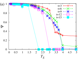
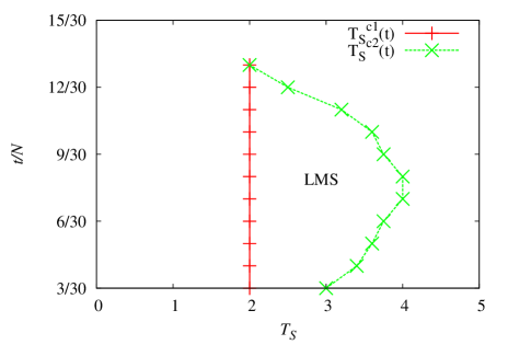
Next, we change the number of target spins $t$ while fixing $N$ at 30. Fig. 9 shows (a) the fitness, (b) the energy, and (c) the frustration parameter $\Phi_{2}$, at $N=30$ and $3\leq t\leq 15$. The threshold temperature $T_{S}$ at which the fitness value decreases rapidly increases as $t$ increases from a small value to 9 and decreases for larger $t$. The $T_{S}$-dependence of the energy shows non-monotonic behavior, indicating the existence of the local Mattis states for all the values of $t$ studied here. Similar to the threshold temperature obtained from the fitness value, the temperature at which the energy takes a minimum value shows non-monotonic behavior as $t$ increases. Further, the range of the plateau with $\Phi_{2}=1$ is maximized at $t=7$ and 8. Eventually, the plateau vanishes at $t=12$ at least. The PM phase, where the adaptation is not acquired, extends toward the lower temperature region with an increase in $t$; the LMS phase becomes narrower as $t$ increases. Fig. 9 shows that the LMS exists only up to $t\hskip 3.00003pt\raisebox{1.72218pt}{$<$}\raisebox{-3.01385pt}{$\sim$}\hskip 3.00003pt0.4N$, and for $t>0.4N$, a direct transition from the SG to PM phase occurs with an increase in $T_{S}$. The LMS region in which robustness and high fitness can be achieved is largest at $t\sim N/4$. These findings indicate that there exists an upper limit of $t$ over which the local Mattis states cannot be obtained and that there exists a suitable value of $t$ for stabilizing the local Mattis states for a wide range of $T_{S}$. The above simulation results are summarized in Fig. 10, where the region of local Mattis state is displayed in the $t/N-T_{S}$ plane, by fixing $N$ and $T_{J}$ at 30 and $0.5\times 10^{-3}$, respectively.

Figure 10: (color online) $t/N-T_{S}$ diagram of the domain where the local Mattis states are found at $N=30$ and a fixed $T_{J}=0.5\times 10^{-3}$. The points on the boundary of the domain are estimated by the values of $T_{S}$ at which $\Phi_{2}$ drops from 1, as in Fig. 9(c), and the line is guide to eye.

Finally, we remark on the equilibration time of the evolutional dynamics of $\bm{J}$ to achieve an adapted state, by varying the value of $t$. At a fixed $T_{J}$, the time scale increases with the increase of $t$, even for a fixed size $N$. Particularly, this increase is significant in the SG phase, while it is moderate in LMS phase. This might remind us of slow relaxation of the phenotype dynamics discussed in the previous section.

IV Fitness landscape

We now explain why mutational robustness is realized only in the intermediate range of temperatures $T_{S}.$ We do so by performing a statistical-mechanical calculation of the number of fitted states in order to obtain a sketch of the fitness landscape for $\bm{J}$. We estimate the degeneracy of the states with highest fitness as $T_{S}\to 0$. Let $W(E_{n}(\bm{J}))$ and $W_{\Psi}(E_{n}(\bm{J}))$ be the number of $n$-th excited states and the number of the target configurations of $n$-th excited states for a given $\bm{J}$. Then, the fitness in the limit as $T_{S}\to 0$ is given by

$$\Psi(\bm{J},T_{S}) =\frac{\sum_{n}W_{\Psi}(E_{n}(\bm{J}))e^{-\beta_{S}E_{n}(\bm{J})}}{\sum_{n}W(E_{n}(\bm{J}))e^{-\beta_{S}E_{n}(\bm{J})}}\equiv\frac{Z_{\Psi}(\bm{J},T_{S})}{Z(\bm{J},T_{S})}$$

$$\longrightarrow\frac{W_{\Psi}(E_{0}(\bm{J}))}{W(E_{0}(\bm{J}))}.$$ (11)

Accordingly, as $T_{S}\rightarrow 0$, the highest fitness, i.e., unity, is achieved if and only if $\bm{J}$ satisfies the condition $W_{\Psi}(E_{0}(\bm{J}))=W(E_{0}(\bm{J}))$. In fact, a large number of $\bm{J}$ satisfy this condition besides the local Mattis state. For example, let us consider a Mattis state $\bm{J}$ with no frustration at all and introduce several changes in the sign of the bonds between target spins $\bm{J}_{tt}$, target and non-target spins $\bm{J}_{to}$, and non-target spins $\bm{J}_{oo}$. This procedure, if applied only to the bond flips to $\bm{J}_{oo}$, produces the local Mattis states.

Figure 11: (color online) (a) The $T_{S}$-dependence of the fitness of the Mattis state (bold line, $\Phi_{1}=\Phi_{2}=\Phi_{3}=1$), one of the local Mattis states (dashed line, $\Phi_{1}=\Phi_{2}=1,\Phi_{3}=0.89$), and one of the target-frustrated states (dotted line, $\Phi_{1}=0.333,\Phi_{2}=1,\Phi_{3}=0.89$), plotted on the left axis. The dashed-dotted line represents the difference $\Delta$ between the fitness of the Mattis state and that of the target-frustrated state; $\Delta$ is plotted on the right.
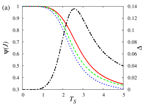
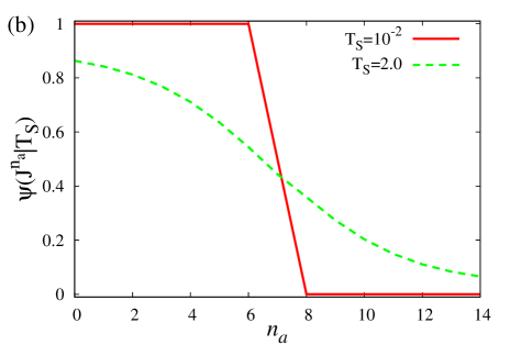
(b) The fitness of $\tilde{\bm{J}}^{n_{a}}$ adapted at $T_{S}=10^{-2}$ (solid line) and $T_{S}=2.0$ (dashed line) with $N=15$ and $t=3$, plotted as a function of the number $n_{a}$ of flipped bonds of $\tilde{\bm{J}}^{n_{a}}$. At low $T_{S}$, the fitness decreases rapidly for $n_{a}=7$ and decreases gradually at intermediate $T_{S}$.

First, we calculate the fitness of the Mattis states ($\Phi_{1}=\Phi_{2}=\Phi_{3}=1$), and we consider representative examples of the local Mattis states ($\Phi_{1}=\Phi_{2}=1$,$\Phi_{3}\neq 1$) and target-frustrated states that have frustration among the target spins and hence $\Phi_{1}\neq 1$. Their fitness is given as the ratio of the “conditioned partition function” $Z_{\Psi}(\bm{J})$ and the partition function $Z(\bm{J})$, as given by Eq. (11). The location of the frustrations does not influence the partition function, but it influences $Z_{\Psi}(\bm{J})$. To determine their fitness function, we should derive the partition functions $Z(\bm{J})$ and $Z_{\Psi}(\bm{J})$ for three types of $\bm{J}$.

At first, the partition function of $\bm{J}$ with $x$ frustrated interactions, $Z(x,T_{S})$ is given as

$$Z(x,T_{S})=2c(x)\sum_{i=0}^{x}C_{i}^{x}f(i,N),$$ (12)

where

$$f(i,N)=\Big{(}4e^{\frac{2\beta_{S}}{\sqrt{N}}}\sinh(\frac{2\beta_{S}}{\sqrt{N}})\Big{)}^{i}\sum_{n=i}^{N-i}e^{-\frac{\beta_{S}}{\sqrt{N}}(N-n)n}C_{n-i}^{N-2i},$$ (13)

and $c(x)=e^{\beta_{S}(-2x+C_{2}^{N})/\sqrt{N}}$. This expression is valid for the case where there is at most one flipped bond at each site. Therefore, $x$ should be less than $N/2$, and the expression Eq. (12) is efficient, independent of how to assign the value $x$ for $\bm{J}_{tt}$, $\bm{J}_{to}$, and $\bm{J}_{oo}$.

Next, the conditioned partition function of the local Mattis state with $x$ frustrated $\bm{J}_{oo}$ interactions (denoted as $Z_{\Psi}^{LMS}(x,T_{S})$) is given as

$$Z_{\Psi}^{LMS}(x,T_{S})=2c(x)\sum_{i=0}^{x}C_{i}^{x}f(i,N-t).$$ (14)

This expression is valid for the case where there is at most one flipped bond at each site. Accordingly, $x$ should be less than $(N-t)/2$. The fitness of the local Mattis states with $x$ frustrated interactions in $\bm{J}_{oo}$ is given as $Z_{\Psi}^{LMS}(x,T_{S})/Z(x,T_{S})$. Furthermore, the conditioned partition function of the target frustrated states that have $y$ frustrations in $\bm{J}_{tt}$ (implying $\Phi_{1}\neq 1$) and $x$ frustrations in $\bm{J}_{oo}$ (denoted as $Z^{TF}(x,y,T_{S})$), is derived from Eq. (13). When a bond between a pair of target spins is flipped from the Mattis state and frustration is generated among the target spins, the energy of the target configuration increases by $2/\sqrt{N}$; therefore,

$$Z_{\Psi}(x,y,T_{S})=Z_{\Psi}^{LMS}(x,T_{S})\times e^{-\frac{2\beta_{S}}{\sqrt{N}}y},$$ (15)

where we again consider that each target spin is connected at most one flipped bond and $y=1,\cdots,t/2$. The partition functions of the target-frustrated states with $x$ frustrated $\bm{J}_{oo}$ bonds and $y$ frustrated $\bm{J}_{tt}$ bonds are given by $Z(x+y,T_{S})$, and their fitnesses are given by $Z_{\Psi}^{TF}(x,y,T_{S})/Z(x+y,T_{S})$.

Fig. 11 shows the $T_{S}$-dependence of the typical fitness values for Mattis, local Mattis, and target-frustrated states. The difference between the fitness of the target-frustrated state and that of the Mattis state, which is denoted as $\Delta$, is also plotted as a function of $T_{S}$. The value of fitness always approaches unity as $T_{S}\to 0$, whereas such degeneracy is split by an increase in $T_{S}$. From the difference in fitness between the Mattis and the target-frustrated states, $\Delta,$ the ratio of the probabilistic weight between these states is obtained as $\exp(\beta_{J}\Delta)$. This suggests that fewer frustrated $\bm{J}$ states around the target, i.e., the local Mattis states, are preferentially selected only at the intermediate temperature.

Next, we introduce frustration into $\bm{J}_{to}$ and denote the constructed $\bm{J}$ as $\tilde{\bm{J}}_{t}^{n_{a}}$, where the superscript $n_{a}$ represents the number of altered bonds and the subscript $t$ represents the condition in which the altered bonds exist between the target and non-target spins, i.e., $\bm{J}_{to}$. Therefore, the frustration parameter $\Phi_{2}$ for $\bm{J}_{to}$ of the state $\tilde{J}_{t}^{n_{a}}$ does not equal 1. The state $\tilde{J}_{t}^{0}$ is simply the original Mattis state, which has the highest fitness, whereas for $n_{a}=N-1$, direct computation shows that the fitness is the least. Again, from a straightforward calculation, it can be shown that the fitness of $\tilde{J}_{t}^{n_{a}}$ remains to be the highest fitness up to $n_{a}\leq N/2$. Hence, there is a region in the $\bm{J}$-state space connected by a single point mutation (change of sign in a single element in $\bm{J}$) in which the fitness retains its highest value. We refer to this region as the neutral spaceAncel and Fontana (2000); Ciliberti et al. (2007); Nimwegen et al. (1999), in the sense that a mutation within the region is neutral. Note that in addition to this construction, there is more degeneracy among the fittest $\bm{J,}$ as shown in Fig. 11(a).

We have computed how the fitness decreases as $\bm{J}$ is changed to leave the neutral space, for $T_{S}\rightarrow 0$. In Fig. 11(b), the fitness of $\tilde{J}_{t}^{n_{a}}$ is plotted as a function of the number of altered bonds $n_{a}$. By just a single point mutation, the fitness decreases suddenly to its lowest value at some $n_{a}$. This implies the existence of a clear edge in the neutral space. The genotype located at the edge of the neutral space is not robust to mutation. It is obvious that the Mattis state, i.e., the genotype located at the center of the neutral space, is robust to mutation. However, since the fitness of genotypes is constant throughout the neutral space, both the robust genotypes at the center of the neutral space and the non-robust genotypes at the edge are selected with equal weight. Then, there is no selection pressure to eliminate genotypes that are at the edge of the neutral space. Although complete degeneracy holds only for $T_{S}\rightarrow 0$, the above argument is valid for sufficiently low temperatures, and therefore, the robustness to mutation cannot be expected to exist in the spin-glass phase at low $T_{S}$. This is also related to the fact that long time scale for equilibration in the evolutional dynamics is required in the spin-glass phase. As shown in Fig. 11(b), the fitness value around an adapted $\bm{J}$ decreases abruptly against the mutation. The number of $\bm{J}$ configurations on the plateau with $\Psi=1$ that appear at low $T_{S}$ is roughly estimated as $2^{N-t}$ because of the gauge transformations for $N-t$ sites, while the total number of possible $\bm{J}$ configurations is $2^{N^{2}}$. The ratio $2^{N-t}/2^{N^{2}}$ is strongly suppressed as $N$ increases. This implies that the evolution of $\bm{J}$ hardly finds the plateau by the local update.

Figure 12: (color online) Schematic representation of the fitness landscape and the probability distribution of the robustness to mutation estimated from the fitness landscape.
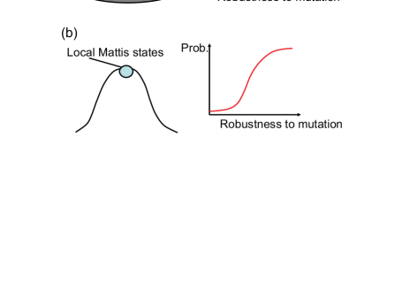
(a) At low $T_{S}$, the genotypes that satisfy the condition $W_{\Psi}(E_{0}(\bm{J}))=W(E_{0}(\bm{J}))$ exist in the neutral space, where the fitness attains its highest value. The local Mattis states also exist in the neutral space, but they constitute a negligible fraction compared to the frustrated genotypes. The neutral space is surrounded by non-adapted genotypes with sharp boundaries, as in Fig. 11(b). The genotypes around the edge of the neutral space that have very low robustness to mutation survive in an evolutionary sense, similar to the robust genotypes located at the center of neutral space, that are much fewer in number.
(b) For $T_{S}$ with $T_{S}^{c1}\leq T_{S}\leq T_{S}^{c2}$, the degeneracy observed at low values of $T_{S}$ is split, and the local Mattis states have the highest fitness. The fitness of the local Mattis state decreases continuously with increasing mutation. There is a correlation between fitness and robustness, i.e., the local Mattis state with the highest fitness is the most robust to mutation, and the robust genotypes are selected preferentially.

In contrast, at intermediate $T_{S}$, the fitness landscape is not neutral. For example, the fitness of $\tilde{\bm{J}}_{t}^{n_{a}}$ gradually decreases from its highest value with increasing $n_{a}$, as shown in Fig. 11(b). There is selection pressure toward the genotype with $n_{a}=0$. The genotypes with larger $n_{a}$ have both lower robustness to mutation and lower fitness, but less of such genotypes are selected. Hence, the evolution toward higher fitness also induces robustness to mutation, as a result of the correlation between fitness and robustness.

On the basis of the above argument, schematic representations of the fitness landscape at low and intermediate $T_{S}$, together with the distribution of mutational robustness, are shown in Fig. 12(a) and (b), respectively. The mutational robustness at an intermediate temperature observed in MC simulations, as described in the previous section, is thus interpreted as a consequence of the evolution of the fitness landscape at such temperatures.

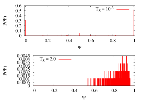
To confirm this schematic picture of the fitness landscape, we have numerically obtained the fitness distribution of mutated $\bm{J}$s around the adapted $\bm{J}$. Here we have computed the fitness values $\Psi$ for $\bm{J}$s mutated from the adapted $J$ with the mutation rate $\mu=0.1$. In Fig. 13, we have plotted the distribution of fitness values at $T_{S}=10^{-3}$ and $T_{S}=2.0$ for $N=15$ and $t=3$. As shown, the fitness distribution of mutated $J$s at low $T_{S}$ has two peaks at $\Psi=1$ and $0$. Hence some mutations are neutral, while others result in a sharp drop in the fitness to its minimal values. In contrast, the fitness of the mutated $\bm{J}$s at the intermediate $T_{S}$ is broadly distribute around 0.8. This result supports the schematic fitness landscape in Fig. 12.

Figure 13: The fitness distribution of mutated $\bm{J}$ with mutation rate $\mu=0.1$, which are generated from the evolved genotypes at $T_{S}=10^{-3}$ and at $T_{S}=2.0$ at $N=15$. The distribution is obtained by 100 types of mutated $\bm{J}$.

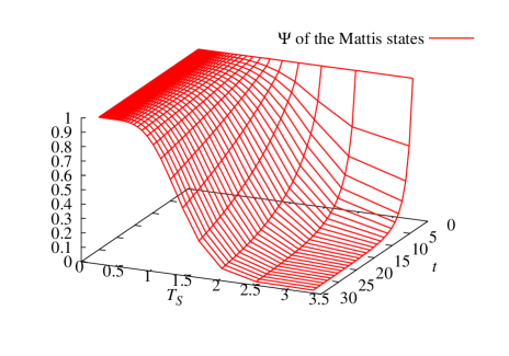
At the intermediate $T_{S}$, it has been shown that the LMS phase vanishes at sufficiently large $t$ as seen in Fig. 9(c). This could be understood by the $T_{S}$ and $t$-dependence of the fitness of the Mattis state. The fitness of the Mattis state at $N=30$ is plotted in Fig. 14, which is obtained from Eq. (12) and Eq. (14). The fitness of the Mattis state as well as the LMS one at the intermediate temperature region decreases as $t$ is increased. As shown in Fig. 9(a), the fitness value decreases rapidly with $T_{S}$ as $t$ increases. The drop with the increase of $T_{S}$ is more prominent for larger $t$, and thus the temperature interval to support the LMS gets narrower with the increase of $t$, and is expected to disappear for large $t$.

Figure 14: $T_{S}$- and $t$-dependence of the fitness $\Psi(T_{S},t)$ of the Mattis state at $N=30$.

V Conclusions and Discussions

We have considered the evolution of a Hamiltonian system to generate a specific configuration for target spins that captures the basic features required to study the evolution. In this study, we adopted a Markov process, which is given by temperature $T_{J}$ and fitness $\Psi(\bm{J})$, for evolutional dynamics. By performing numerical simulation, we found that a specific subset of $\bm{J}$ with low energy and high fitness is evolved at an intermediate $T_{S}$ and low $T_{J}$. From the statistical-mechanical viewpoint, we focused on frustration and found that the interactions $\bm{J}$ that evolved at the intermediate $T_{S}$ are less frustrated. We called these $\bm{J}$ the local Mattis states. In general, the less frustrated $\bm{J}$ states are robust to mutation. Hence, the robustness of evolving states to mutation is realized at intermediate temperatures $T_{S}^{c1}\leq T_{S}\leq T_{S}^{c2}$. In other words, robustness to thermal noise introduces mutational robustness; this has also been recently discussed for gene regulation network modelsKaneko (2007). The relevance of thermal noise to robust evolution is thus demonstrated.

The mechanism by which the mutational robustness is achieved could be understood by a statistical-mechanical argument. The $T_{S}$-dependence of the fitness landscape was determined by explicitly calculating the fitness $\Psi(\bm{J})$ for a typical case. It was found that the correlation between fitness and mutational robustness is generated at intermediate $T_{S}$, while it disappears at sufficiently low $T_{S}$. Hence, the mutationally robust interactions $\bm{J}$ are obtained as a result of the selection under a certain level of noise. The evolution of the mutational robustness at the intermediate $T_{S}$ is confirmed by applying statistical-mechanical theory.

We also found that for the interactions evolved at the intermediate $T_{S}$, the relaxation to equilibrium progresses smoothly without being stuck at metastable states. For protein folding, such an energy landscape was proposed in terms of the consistency principle by Go Go (1983) and as a funnel-landscape by Onuchic et al. Onuchic and Wolynes (2004). The funnel energy landscape has no ruggedness around the folded state, in contrast to the spin-glass state. On the other hand, far from the folded state, the ruggedness in the landscape remains; this is different from the global attraction in the ferromagnetic or Mattis state. We note that the landscape in a local Mattis state that is generated as a result of evolution at $T_{S}^{c1}\leq T_{S}\leq T_{S}^{c2}$ is such a funnel landscape, as there is no frustration around the target spins, whereas frustration around non-target spins can result in ruggedness in the landscape far from the target configuration. Indeed, such a smooth and quick relaxation process is observed only for $T_{S}^{c1}\leq T_{S}\leq T_{S}^{c2}$, whereas the relaxation is often stuck at metastable states for a system evolved below $T_{S}^{c1}$. On the basis of this correspondence between the funnel landscape and the local Mattis state, we expect that the funnel landscape is characterized by a state with $\Phi_{1}=\Phi_{2}=1$.

Biological systems have evolved and functioned at a range of temperatures. Recall that for a Hamiltonian evolved with $T_{S}<T_{S}^{c1}$, a large number of time steps is required to reach a spin configuration having the highest fitness, and the number of steps seems to increase with the number of total spins. High fitness is not achieved for a low-temperature region within a biologically acceptable time span, i.e, within a single generation. Accordingly, adaptive evolution is possible only when sufficient thermal noise is present; this corresponds to $T_{S}>T_{S}^{c1}$.

We have found that the funnel-like landscape evolves in such biologically relevant temperature regions. In fact, such a landscape is commonly observed not only in protein folding but also in gene expression dynamics Kaneko (2007); Li et al. (2004) and in the morphogenesis of multicellular organisms Kaneko et al. (2008). Our result implies that a landscape that allows smooth relaxation dynamics toward the target phenotype, such as the above-mentioned landscape, is realized as a consequence of dynamics that are robust to thermal noise as well as to mutation. We expect that this type of landscape that results from robustness can be found in general in biological evolution. It will not be restricted to Hamiltonian dynamics for protein folding; rather, it will be generally applicable in developmental dynamics. Indeed, recent studies on the evolution of the gene regulation network also demonstrate that the funnel-type dynamics evolve at the intermediate range of noise amplitude values Kaneko (2007, 2008). Our results may explain the ubiquity of such funnel-like dynamics in evolved biological systems.

Although the frustration measure in the present paper is not directly applied to the gene regulation network, the transition to the robust developmental landscape is common. It will be interesting to study the similarities and differences in the transitions in the spin Hamiltonian model presented here and the dissipative gene expression dynamical model.

It is also interesting that there is an optimal number of target spins for achieving the local Mattis state with a funnel energy landscape over a wide range of temperatures. The number of non-target spins $N-t$ controls the redundancy of the system. If $t$ is too small, the target configurations will be more easily perturbed by non-target spins, and fitted states will be less robust to the thermal noise. On the other hand, if it is too large, such $\bm{J}$ configurations with high fitness are too much limited in the whole configurations, and hence it will not be easily accessed or may be destabilized by mutation. The existence of an appropriate number of redundant spins is important to achieve robustness. Indeed, in proteins, amino-acid residues that are responsible for a function are limited and their number is typically smaller than the number of other proteins. Possible links between redundancy and the evolvability are pointed out in Wagner (2007), but they still wait to be established quantitatively by theoretical analysis. The present demonstration of the optimal fraction of target elements for realizing robust functions will be important in this context.

In this study, we observed transitions at $T_{S}^{c1}$ and $T_{S}^{c2}$. The phase below $T_{S}^{c1}$ corresponds to the spin-glass phase and that above $T_{S}^{c2}$ corresponds to the paramagnetic phase in the context of statistical physics; in contrast, the local Mattis phase between the two phases, which could correspond to the funnel landscape, is a novel discovery in this study. Since a framework of statistical physics of spin systems has been adopted in the present study, the theoretical concepts developed therein, such as replica symmetry breaking, may be applicable in the context developed here to understand this transition. In particular, our model in this study is a variant of spin Hamiltonian systems with two temperatures: one for spin and the other for interactions $\bm{J}$. Theoretical analysis of such systemsPenney et al. (1993); Dotsenko et al. (1994) will be relevant for the analysis of the local Mattis state and mutational robustness that we have discussed in this paper.