Periodic class II methanol masers in G9.62+0.20E

Abstract

We present the light curves of the 6.7 and 12.2 GHz methanol masers in the star forming region G9.62+0.20E for a time span of more than 2600 days. The earlier reported period of 244 days is confirmed. The results of monitoring the 107 GHz methanol maser for two flares are also presented. The results show that flaring occurs in all three masing transitions. It is shown that the average flare profiles of the three masing transitions are similar. The 12.2 GHz masers are the most variable of the three masers with the largest relative amplitude having a value of 2.4. The flux densities for the different masing transitions are found to return to the same level during the low phase of the masers, suggesting that the source of the periodic flaring is situated outside the masing region, and that the physical conditions in the masing region are relatively stable. On the basis of the shape of the light curve we excluded stellar pulsations as the underlying mechanism for the periodicity. It is argued that a colliding wind binary can account for the observed periodicity and provide a mechanism to qualitatively explain periodicity in the seed photon flux and/or the pumping radiation field. It is also argued that the dust cooling time is too short to explain the decay time of about 100 days of the maser flare. A further analysis has shown that for the intervals from days 48 to 66 and from days 67 to 135 the decay of the maser light curve can be interpreted as due to the recombination of a thermal hydrogen plasma with densities of approximately $1.6\times 10^{6}~{}\mathrm{cm^{-3}}$ and $6.0\times 10^{5}~{}\mathrm{cm^{-3}}$ respectively.

1 Introduction

Although class II methanol masers are now generally accepted to be exclusively associated with massive star forming regions (see eg. Ellingsen, 2006; Xu et al., 2008), it is not yet clear how much can be learned about the star formation environment from the masers. Underlying this uncertainty is the fact that it is difficult to determine where in the circumstellar environment the masers operate based solely on the spatial distribution and velocity structure of the masers (Beuther et al., 2002). In the past very little attention has been given to the time domain aspect of the masers. Various authors (see eg. MacLeod et al., 1993; Caswell et al., 1995; Moscadelli & Catarzi, 1996; Goedhart et al., 2002; Niezurawska et al., 2002; Goedhart et al., 2003, 2004; Goedhart et al., 2005a) have studied the variability of the 6.7 and 12.2 GHz masers over various periods of time and have found that variability is a common feature amongst these masers. The most systematic study on the variability of 6.7 GHz masers to date was done by Goedhart et al. (2004) using the Hartebeesthoek Radio Astronomy Observatory (HartRAO) 26-m telescope, revealing a wide variety of time-dependent behaviour in the masers. Six out of their list of 54 sources were identified as periodic, with periods ranging from 133 to 504 days (Goedhart et al., 2007). Of particular interest here are the periodic masers in the star forming region G9.62+0.20E which show repeated flaring activity with a period of about 244 days (Goedhart et al., 2003; Gaylard & Goedhart, 2007)

The star forming region G9.62+0.20 has been the object of study by a number of authors. Garay et al. (1993) mapped this region with the VLA at 1.5, 4.9 and 15.0 GHz and identified five extended, compact and ultracompact (UC) H II regions, labelled A - E. A striking feature in this star forming complex is the near perfect alignment of various tracers (masers, hot molecular clumps and UC H II regions) of star forming activity extending between components C and D, with component E lying between C and D (see Hofner et al., 1994). Hofner et al. (1994) interpreted the overall morphology of this star forming region as suggestive of induced star formation progressing from the most evolved H II region (component A) with the most recently formed stars located in the linear structure. The methanol masers in the star forming complex are associated with components D and E and are in the literature also referred to as G9.619+0.193 and G9.621+0.196 respectively (Phillips et al., 1998). For component E, the masers have a maximum linear extent of about 566 AU (2.75 milliparsec) based on the 12.2 GHz observations of Goedhart et al. (2005b) and using a distance of 5.15 kpc (A. Sanna et al., in preparation).

Component E shows all the signs of a very early phase of massive star formation. According to Hofner et al. (1996) the continuum emission follows a power law with a spectral index of $1.1\pm 0.3$ between 2 cm and 2.7 mm, which can be interpreted to be due to either an ionized spherical stellar wind or a spherical homogeneous UC H II region with an excess of dust emission at 2.7 mm. If interpreted as an UC H II region, the size of the H II region is only 2.5 mpc and is excited by a B1 ZAMS star (Hofner et al., 1996). Franco et al. (2000) quote a slightly flatter spectral energy distribution between 8.4 and 110 GHz, with a spectral index of $0.95\pm 0.06$ which they attribute to a density gradient proportional to $r^{-2.5}$. Using the 1.3 cm data of Testi et al. (2000) for G9.62+0.20E, Franco et al. (2000) derives an electron density of about $6\times 10^{5}~{}\mathrm{cm^{-3}}$ which could rise to above $10^{6}~{}\mathrm{cm^{-3}}$ in a uniform core region. Taken together with the size of the H II region, G9.62+0.20E qualifies as a hypercompact H II region, implying a very early phase of massive star formation.

Component E is also well defined in a number of sulphur and nitrogen bearing molecules as well as in some organic molecules (Su et al., 2005). Near-infrared imaging of the star forming region shows emission at components B, C and E (Testi et al., 1998). Persi et al. (2003) subsequently found that the NIR source near component E has the colours of a foreground star. De Buizer et al. (2005) find weak emission at 11.7 $\mu$m towards the radio component E.

In this paper we present further monitoring data on G9.62+0.20E for methanol masers at 6.7, 12.2, and 107 GHz. We present various analyses of the data and consider a possible explanation for the variability of the masers.

2 Observations and data reduction

HartRAO observations: Observations at 6.7 GHz and 12.2 GHz were made with the 26-m Hartebeesthoek telescope. Both receivers provide dual circular polarization. The system temperatures at zenith are typically 60 K at 6.7 GHz and 100 K at 12.2 GHz. The spectrometer provides 1024 channels per polarization, and the bandwidths used for spectroscopy of 1 MHz at 6.7 GHz and 2 MHz at 12 GHz provide spectral resolutions of 0.044 and 0.048 km s^-1 respectively.

For spectroscopic observing, the telescope pointing error was determined through five short integrations at the cardinal half power points of the beam and on source. The on-source spectra were scaled up by determining the amplitude correction from the pointing error using a Gaussian model for the main beam.

Calibration was based on monitoring of 3C123, 3C218 and Virgo A (which is bright but partly resolved), using the flux scale of Ott et al. (1994). The antenna temperature from these continuum calibrators was measured by drift scans. Pointing errors in the north-south direction were measured via drift scans at the beam half power points, and the on-source amplitude was corrected using the Gaussian beam model. The bright methanol maser source G351.42+0.64, which previous monitoring has shown to exhibit only small variations in the strongest features (Goedhart et al., 2004), was observed in the same way as G9.62+0.20 to provide a consistency check on the spectroscopy. These sources were observed frequently, usually on the same days as G9.62+0.20.

ARO 12m observations: The observations with the ARO 12m telescope were done from December 3, 2003 to June 25, 2004 to observe cycle 8 and from January 14, 2005 to April 22, 2005 to observe cycle 9. The peak for cycle 8 was expected in early July 2004. Poor atmospheric conditions forced any further observations to be abandoned after June 2004. The onset of flare 9 was expected to occur around February 7, 2005 with a peak between March 7 - 13 and to decay to its low state by middle April 2005. The receivers used were dual-channel SIS mixers operated in single-sideband mode. The backends were filter banks with 100kHz and 250 KHz resolution. The observing frequency was 107.01385 GHz. Each observing run lasted about three hours, during which regular positional checking on planets were done.

DR-21 was used as calibrator as well as a reference source and was observed in spectral line mode. Data reduction was done with the CLASS package. Fig.1 shows the time series for DR-21.

Figure 1: Time series for the continuum emission of DR-21 at 107 GHz

The results are for the 250 KHz resolution and each point is the average over all channels. We estimated the flux density of DR-21 at 107 GHz using the continuum spectrum given by Righini et al. (1976), which gives a flux density of 16.7 Jy. For each observing run an appropriate conversion factor was calculated and applied to the corrected antenna temperature of G9.62+0.20E.

3 Results and analysis

The average or representative spectra for the three maser transitions are shown in Fig. 2. It is seen that, whereas for the 6.7 and 12.2 GHz spectra the strongest feature is located at about 1.3 $\mathrm{km~{}s^{-1}}$, the corresponding feature in the 107 GHz spectrum is the weaker maser feature. The 107 GHz spectrum also shows a broad thermal component. G9.62+0.20E has in the past been observed at 107 GHz by Val’tts et al. (1995, 1999) and Caswell et al. (2000). The average 107 GHz spectrum in Fig. 2 resembles the result of Caswell et al. (2000). The observations of Val’tts et al. (1995, 1999) show only one maser feature at -0.57 $\mathrm{km~{}s^{-1}}$ and also no broad thermal component.

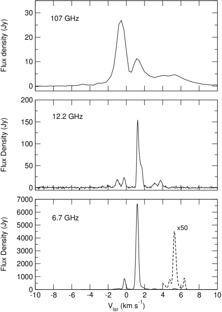
Figure 2: Representative spectra for the masers at 6.7, 12.2 GHz. The 107 GHz spectrum is an average taken over all observations. The features at 5.3 and 6.4 $\mathrm{km~{}s^{-1}}$ in the 6.7 GHz spectrum are associated with G9.62+0.20D.

The full time series for all the identifiable features in the 6.7 and 12.2 GHz spectra are shown in Figs. 3 and 4. For the 6.7 GHz maser, eleven different features could be identified in the single dish spectrum and ten for the 12.2 GHz maser. The time series covers about 2670 days and 13 flares. Inspection of Fig. 3 shows that while there are some similarities in the time series of some of the 6.7 GHz maser features, there also are some significant differences.

The strongest varying 12.2 GHz masers are significantly more variable than the strongest varying 6.7 GHz masers. To quantify the variability we calculated the relative amplitude, defined as

$$R=\frac{S_{max}-S_{min}}{S_{min}}=\frac{S_{max}}{S_{min}}-1$$ (1)

for a number of features in the three transitions. The results are given in Table 1. The errors indicate the spread in the relative amplitudes for the last six flares in the time series. No error could be given for the single 107 GHz flare that has been monitored. The 12.2 GHz masers are indeed significantly more variable than the 6.7 and 107 GHz masers while the relative amplitudes of the 6.7 and 107 GHz masers are approximately the same.

Table 1: Relative amplitudes (eq. 1) for selected masers at 6.7, 12.2 and 107 GHz

6.7 GHz		12.2 GHz		107 GHz
Velocity	Relative	Velocity	Relative	Velocity	Relative
$\mathrm{km\,s^{-1}}$	amplitude	$\mathrm{km\,s^{-1}}$	amplitude	$\mathrm{km\,s^{-1}}$	amplitude
1.18	0.26 $\pm$ 0.04	1.25	2.0 $\pm$ 0.4	1.14	0.31
1.84	0.32 $\pm$ 0.05	1.63	2.4 $\pm$ 0.3
2.24	0.33 $\pm$ 0.04

Figures 3 and 4 also show that the regular flaring does not occur in all of the 6.7 and 12.2 GHz maser features. For the 12.2 GHz masers it is seen that the flaring behaviour is limited to three features namely $+1.25~{}\mathrm{km\>s^{-1}}$, $+1.63~{}\mathrm{km\>s^{-1}}$ and $+2.13~{}\mathrm{km\>s^{-1}}$. The strongest flaring occurs at +1.25 and +1.63 $\mathrm{km\>s^{-1}}$. These are also the strongest two features in the maser spectrum. The absence of flaring behaviour outside the above velocity range is quite obvious. Because of the smaller variability of the 6.7 GHz masers the question of which features are flaring is not as simple as for the 12.2 GHz masers. Simple visual inspection suggests that flaring occurs for the features at -0.2, +1.2, +1.8, and +2.2 $\mathrm{km\>s^{-1}}$.

It is noteworthy that the most variable and brightest 12.2 GHz masers, at +1.63 and +1.25 $\mathrm{km\>s^{-1}}$, lie close to each other at the northern end of a north-south chain of maser features as seen in the high resolution maps of Goedhart et al. (2005b). As already pointed out, these are also the two brightest masers in the 12.2 GHz spectrum. The maser features that show no periodic flaring lie significantly offset to the south from the above two features.

We also checked for periodic variations in the light curves using the Lomb-Scargle periodogram (Scargle, 1982) and Davies’ L-statistic (Davies, 1990). For the 12.2 GHz masers both methods confirm the existence of a periodic signal with period 244 days in the light curves of the $+1.25~{}\mathrm{km\>s^{-1}}$, $+1.63\mathrm{km\>s^{-1}}$ and $+2.13~{}\mathrm{km\>s^{-1}}$ features at a very high level of significance. For the 6.7 GHz masers the periodograms were significantly more complicated than that of the 12.2 GHz masers. A full analysis and discussion of the periodograms falls outside the scope of the present paper and will not be discussed here. Within the context of the present paper it is necessary to note that for the 12.2 GHz masers, periodic (regular) flaring is observed only in three features. For the 6.7 GHz masers, flaring behaviour is strongest also for only a subset of the maser features, some of which coincide in velocity with the 12.2 GHz masers that show flaring behaviour.

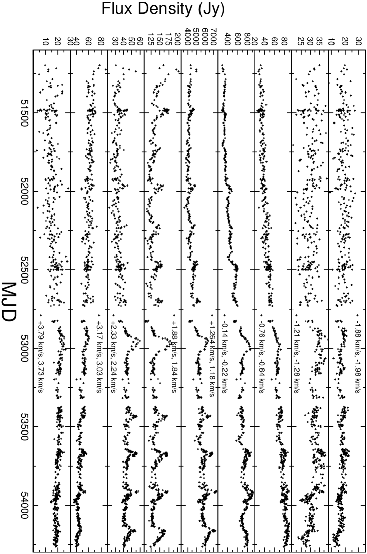
Figure 3: 6.7 GHz time series

Figure 4: 12.2 GHz time series

In Fig. 5 we show the time series for cycles 9 and 10 for which the 107 GHz masers have also been monitored. The vertical dashed lines give the position of the peak of the flare at 12.2 GHz for the 1.25 $\mathrm{km\>s^{-1}}$ feature. For cycle 9 the scatter in the 107 GHz data is quite large and, although there might be a slight hint of a rise in the flux density towards the expected time when the flare was at its peak, no clear sign of a flare can be identified. The reason for the large scatter in the data is most probably the poor atmospheric conditions that prevailed at that time and which led to the termination of the monitoring for cycle 9.

Closer inspection of the time series in Figs. 3, 4, and 5 suggests that the flare profiles for the 6.7, 12.2 and 107 GHz masers might be different. To investigate to what extent the flare profiles are similar we first considered the average flare profiles by calculating the normalized profile

$$J(t)=\frac{S(t)-S_{min}}{S_{max}-S_{min}}$$ (2)

for the +1.25 $\mathrm{km\>s^{-1}}$ feature of the 12.2 GHz spectrum and for the corresponding feature at 6.7 GHz. For both these features a 30 point running average was used after detrending the time series and folding of the data modulo the period of 244 days. The 107 GHz data for the one flare were scaled accordingly. The results are shown in Fig. 6. In spite of the fact that the average profiles do not coincide exactly in time, it is remarkable to note that the profiles seem to be very similar for the three maser transitions.

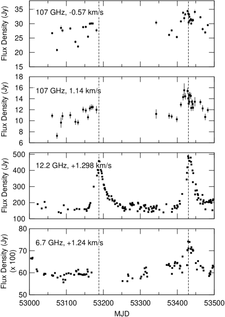
Figure 5: Time series for masers at 6.7, 12.2 and 107 GHz. For the 6.7 and 12.2 GHz masers only one velocity component has been considered. The solid dashed vertical lines indicate the position of the peak of the 12.2 GHz maser.

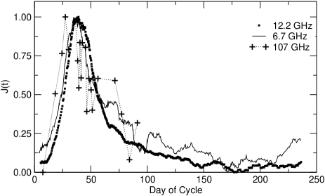
Figure 6: Comparison of the average flare profile for the 1.24 $\mathrm{km~{}s^{-1}}$ feature for the 6.7, 12.2, and 107 GHz masers. For the 6.7 and 12.2 GHz masers the flare profile was obtained from a 30 point running average.

The same analysis as above was also carried out on individual 6.7 and 12.2 GHz flares to examine to what extent individual flares have the same profile. The result is shown in Fig. 7. For clarity only the flares that occured after MJD 52750 are shown and only for the features at 1.25 $\mathrm{km\>s^{-1}}$. In spite of the large errors on the 6.7 GHz data, it is seen that the flare profiles are basically the same, also for individual flares. The similarity of the individual flare profiles suggests that the characteristics of the mechanism underlying the flaring remain the same from flare to flare and that it affects the 6.7 and 12.2 GHz masers in the same way.

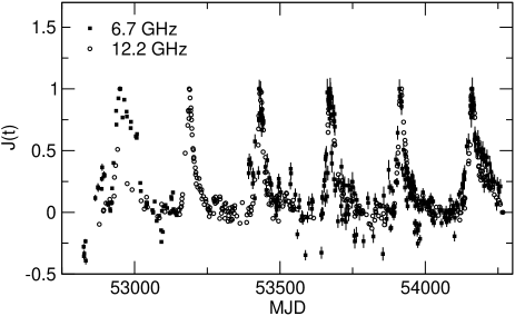
Figure 7: Comparison of the individual normalized flare profiles for the 1.24 $\mathrm{km~{}s^{-1}}$ feature for the 6.7 and 12.2 GHz masers for MJD $>$ 52750

We finally note that within the velocity resolution of the observations, no velocity shifts of the different feature in the maser spectrum could be detected during the flares.

4 Discussion

Goedhart et al. (2005a) briefly considered a number of possible mechanisms that might underlie the flaring behaviour of the masers in G9.62+0.20E. These included: disturbances like shock waves or clumps of matter passing through the masing region; variations in the flux of seed photons or of pump photons due to stellar pulsations; periodic outbursts, or the effects of a binary system. While it is not possible to come to a final conclusion about the origin of the periodicity of the masers with the present data, it is possible to at least exclude certain mechanisms and point to possible explanations for the periodicity.

It has already been noted that the return of the masers to basically the same quiescent level between flares is a strong indication that the masing regions remain unaffected by whatever mechanism underlies the flaring. Mechanisms such as shock waves or clumps of matter passing through the masing region are therefore excluded. This implies that whatever the underlying mechanism for the periodicity, the coupling with the masing regions must be radiative, ie. either through the seed photons or through heating and cooling of the dust that is responsible for the pumping radiation field.

At present the information available on the masers are the single dish light curves (as presented above) and the high resolution interferometric mapping of Goedhart et al. (2005b). We consider the light curve (flare profile) only since in general the light curves of periodic sources contain significant information about the physical processes that are responsible for the observed variability. We also present an analysis that strongly suggests that the decay part of the light curve might be due to the background H II region decaying from a higher to a lower state of ionization. It is necessary to point out here that since the relative positions of the masers with respect to the H II region is not known to milli-arcsecond accuracy, a more complete understanding of all aspects of the variability of the masers in G9.62+0.20E cannot be given here.

For the present discussion we will focus on the strongest maser features and take the average flare profile of the 12.2 GHz masers (Fig. 6) as representative of all flares. The flare profile can be described by a rather steep rise followed by a decaying part lasting about 100 days to eventually reach a minimum (or possibly quiescent) state after which it appears to slowly increase before the next flare starts again. Since, as we have already argued that effects that physically affect the masing region can be ruled out, we are basically left with two possibilities to understand the light curve: stellar pulsation and a binary system.

A comparison of the maser light curves as described above with the light curves of all classes of pulsating stars clearly shows that the maser light curve has a completely different behaviour from that of any class of pulsating stars. In fact, considering the physics of stellar pulsation it is hard to see how to produce a light curve for a pulsating star such that it resembles that of the masers in G9.62+0.20E. For the masers the light curve is strongly suggestive of a flaring state that is superposed on top of a base level emission. Pulsating stars are not in an equilibrium state and therefore do not have such a quiescent state on top of which pulsations or flares are superposed. Explaining the observed maser light curves as being due to pulsation of the central star would therefore appear to be very difficult.

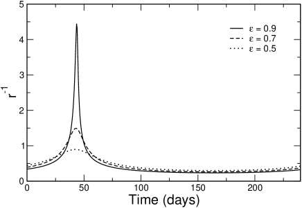
Figure 8: Time dependence of $r^{-1}$ for different eccentricities.

The only alternative is that of a binary system. The light curve does not suggest that we are dealing with an eclipsing effect for the masers. A class of binary systems which potentially can meet the requirement of providing radiative coupling between the source of variability and the masing regions is the colliding-wind binaries. In fact, Zhekov et al. (1994) argued that, given the high binary frequency found in young stars and the observed mass loss rates and wind velocities, supersonically colliding-wind systems, should also be found amongst pre-main sequence binary systems. Although it is not possible with the available data to come to a conclusion here whether or not G9.62+0.20E indeed harbours a colliding-wind binary, it is worth exploring this possibility somewhat more by considering some properties of colliding-wind binaries.

The main ingredient of a colliding-wind binary is the two oppositely facing shocks separated by a contact discontinuity. The postshock temperature is given by $T_{sh}=3mv_{w}^{2}/16k$ (Stevens et al., 1992; Zhekov et al., 1994), where $m$ is the mean mass of the particles that constitute the wind, and $v_{w}$ the wind speed. Given that the central star for G9.62+0.20E is estimated to be of spectral type B1 and using the results of Bernabeu et al. (1989), a wind speed of $800~{}\mathrm{km~{}s^{-1}}$ does not seem to be an unrealistic assumption. Using this value for $v_{w}$ and assuming for simplicity a pure hydrogen wind, a postshock temperature of $\sim 1.5\times 10^{7}$ K is found. Pittard et al. (2005) presented the emissitivity for hot thermal plasmas of temperatures $10^{6}$, $10^{7}$, and $10^{8}$ K, from which an extrapolation to energies below 100 eV suggests that the post-shock gas will emit photons from the visible up to X-ray energies. Using the CHIANTI code (Dere et al., 1997; Landi et al., 2006), we confirmed that this is indeed the case. This range of photon energies obviously includes photons that can heat the inner edge of the circumstellar dust as well as ionizing photons that can cause additional ionization in the H II region, respectively affecting the pumping radiation field and/or the background source of seed photons. Due to the lack of a numerical model it was not possible to calculate expected absolute fluxes of ionizing photons produced at the shocks as well as of photons that can heat the dust. A quantitative evaluation of the effects these photons might have on the H II region and the dust was therefor not possible.

A second property of colliding-wind systems relevant to this discussion, is that the total luminosity at the shock scales like $r^{-1}$, where $r$ is the distance between the two stars (Stevens et al., 1992; Zhekov et al., 1994). Obviously this scaling property implies a modulating effect of the total luminosity at the shock during the orbital motion for eccentric orbits. To investigate the time dependence of $r^{-1}$, we used Kepler’s third law to calculate the semi-major axis for the binary system. For this we used a mass of 17 $\mathrm{M_{\odot}}$ for the ionizing star (spectral type B1) and arbitrarily adopted a mass of 8 $\mathrm{M_{\odot}}$ for the secondary star. Since in Kepler’s third law the semi-major axis depends on the inverse of the third root of the total mass, the final answer is not very sensitive to the mass of the secondary. Using the period of 244 days it then follows that the semi-major axis of the orbit is 2.23 AU. For an elliptic orbit the radial distance between the two stars is given by $r=a(1-e^{2})/(1+e\cos\theta)$ with $a$ the semi-major axis and $e$ the eccentricity. The resulting orbital modulation, for eccentricities of 0.5, 0.7, and 0.9, of the luminosity is shown in Fig. 8 with $r$ in AU. The position of periastron passage has been set at 43.5 days in all three cases.

Combining the above two basic properties of colliding-wind binary systems, it is clear that such systems can provide a periodic source of photons that can heat the circumstellar dust and thereby possibly affect the pumping radiation field for the masers, as well as ionizing photons that can cause additional ionization in the H II region. Although the exact projection of the masers against the H II region in G9.62+0.20E is not known, the work of Phillips et al. (1998) suggests that the H II region might indeed be the source of seed photons for the masers.

Comparison of Fig. 8 with the maser flare profile, however, shows that, even in the case of an eccentricity of 0.5, the observed maser flare profile has a decay time that is significantly longer than what is expected simply from the radiation pulse produced at periastron passage. Within the framework of the colliding-wind binary scenario, the observed decay must then be due to either the cooling of dust or the recombining of the H II region (or parts thereof) from a higher degree of ionization to its pre-flare state.

Using the fact that the dust cooling time is proportional to $T^{-6}$ (Krügel, 2003) for the optical thin case and proportional to $T^{-4}$ in the optically thick case, and that in the optical thin case the typical cooling times for small grains with a temperature of 60 K is about 10 seconds (Krügel, 2003), an upper limit of about 10 hours for the cooling time is found for the optically thick case. Assuming now a grain temperature of 100K and that the cooling time under optically thin conditions is also 10 seconds, which, due to the $T^{-6}$ dependence should actually be less, a cooling time of 1.2 days is found for the optically thick case. Thus, even in the optically thick case the dust cooling time is only a small fraction of the decay time of the maser flare, suggesting that the decay of the maser flare is most probably not due to the cooling of dust.

To investigate the possibility that the decaying part of the maser flare is due to the recombination of the H II region or parts thereof, we note that the recombination time scale of a hydrogen plasma is given by $(\alpha n_{e})^{-1}$ (Osterbrock, 1989), with $\alpha$ the recombination coefficient and $n_{e}$ the electron density. Using $\alpha=2.95\times 10^{-13}~{}\mathrm{cm^{3}s^{-1}}$, characteristic decay times between 40 and 400 days are found for densities between $n_{e}=10^{6}~{}\mathrm{cm^{-3}}$ and $n_{e}=10^{5}~{}\mathrm{cm^{-3}}$. This is significantly longer than the dust cooling time and seems to be able to account for the observed decay time of about 100 days.

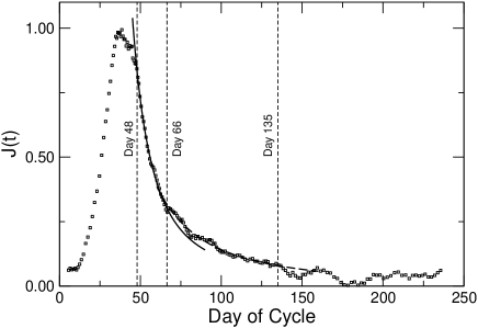
Figure 9: Normalized average flare profile for the 12.2 GHz masers with the solid and dashed lines the fits from eq. 3. The vertical dashed lines indicate the time intervals which was used for the fitting.

In view of these numbers, the question arises whether the decay of the maser flare can indeed be ascribed to a change in the seed photon flux from a recombining thermal plasma. In Appendix A we derive an expression for the time dependence of the electron density in a volume of ionized hydrogen going from a higher level of ionization to a lower equilibrium ionization state, due to the recombination of the plasma. It is shown that in the optically thin case, the intensity of the associated free-free emission decreases with time according to

$$I_{\nu}(t)\propto\left[\frac{1+u_{0}\tanh(\alpha n_{e,\star}t)}{u_{0}+\tanh(\alpha n_{e,\star}t)}\right]^{-2}$$ (3)

with $u_{0}=n_{e,0}/n_{e,\star}>1$. $n_{e,0}$ is the electron density from where the decay starts at time $t=0$, and $n_{e,\star}$ the equilibrium electron density determined by ionization balance for the ionizing stellar radiation. Fitting eq. 3 to the decay part of the flare will give an indication to what extent the decay of the maser flare can be interpreted as being due to the recombination of a hydrogen plasma. An initial non-linear regression analysis using the above time dependence suggested that the decay of the maser flare actually consists of two components that have to be fitted separately. The first component is from days 48 to 66, and the second from days 67 to 135.

Following the discussion in Appendix A, we thus fitted the two components with eq. 3 by systematically varying $n_{e,\star}$. This allowed us to estimate $u_{0}$ and therefore $n_{e,0}=u_{0}n_{e,\star}$, ie. the electron density at the time when the ionization pulse was switched off or when its effect was not significant anymore. For the interval between days 48 and 66 it was found that $n_{e,0}$ varies from $1.57\times 10^{6}~{}\mathrm{cm^{-3}}$ to $2.00\times 10^{6}~{}\mathrm{cm^{-3}}$ for $n_{e,\star}$ ranging from $1.0\times 10^{5}~{}\mathrm{cm^{-3}}$ to $7.0\times 10^{5}~{}\mathrm{cm^{-3}}$. Similarly, for the interval between days 67 and 135, $n_{e,0}$ varies between $6.0\times 10^{5}~{}\mathrm{cm^{-3}}$ and $7.3\times 10^{5}~{}\mathrm{cm^{-3}}$ for $n_{e,\star}$ ranging from $1.0\times 10^{4}~{}\mathrm{cm^{-3}}$ to $2.0\times 10^{5}~{}\mathrm{cm^{-3}}$. For each interval the lower value for the range of $n_{e,\star}$ was chosen such that $n_{e,0}$ is also the solution of eq. 8, ie. the solution for the limiting case when $n_{e,\star}\ll n_{e,0}$. The upper value for the range of $n_{e,\star}$ was chosen to be about one third or half of the value of $n_{e,0}$ obtained for the lower value of the range of $n_{e,\star}$.

In Fig. 9 we show the fit of eq. 3 to each of the two time intervals of the decay of the maser flare for specific values of $n_{e,\star}$ from the abovementioned ranges of values. For days 48 to 66 we used $n_{e,\star}=3\times 10^{5}~{}\mathrm{cm^{-3}}$ and for days 67 to 135 we used $n_{e,\star}=1\times 10^{5}~{}\mathrm{cm^{-3}}$. These two values correspond to $n_{e,0}=1.66\times 10^{6}~{}\mathrm{cm^{-3}}$ and $n_{e,0}=6.36\times 10^{5}~{}\mathrm{cm^{-3}}$, respectively. The quality of the fits is quite remarkable, especially given that a priori there is no information suggesting that the decay of the maser flare might follow the recombination of a thermal hydrogen plasma. The values for $n_{e,0}$ as estimated from the non-linear regression are also what is expected for hypercompact H II regions. In fact, the agreement with the densities quoted by Franco et al. (2000) for G9.62+0.20E is also remarkable. At the least these results are strongly suggestive that the decay of the maser flare might be due to the recombination of an H II region, or parts thereof, from a higher to a lower ionization state. The entire maser flare might therefore be due to changes in the background source.

We also note that within the framework of the hypothesis that the maser flaring is due to changes in the background H II region, day 48 gives an upper limit of the time when the radiative pulse causing the increase in the ionization level, has “switched” off and the H II region is left to decay to its equilibrium level. Referring to Fig. 6 the start of the flare is at about day 10, implying that the full width of the radiative pulse is at most about 38 days. This suggests a rather sharply peaked pulse which is what is qualitatively expected from the colliding-wind binary scenario discussed above.

To what extent the colliding-wind binary scenario is the only one that can explain the maser flaring within the broader framework of binary systems, is not clear yet. Our discussion above does not include the presence of a possible accretion disk or even two accretion disks, as well as outflows. Obviously such scenarios are much more complex, but should nevertheless be able to explain the periodic flaring as well as the shape of the flare profiles. Given the short cooling time of the dust, it follows, if the entire flare profile is due to changes in the pumping radiation field, that the primary driving source of the variable infrared radiation field should basically have the same time dependence as the maser flare profile. Furthermore, the physical process should be rather stable from orbit to orbit to explain the similarity of the flare profiles in the time series. Obviously, monitoring of G9.62+0.20E in the mid-infrared might help resolve this problem.

5 Summary and Conclusion

We presented the results of the monitoring of methanol masers in G9.62+0.20 at 6.7, 12.2, and 107 GHz. Like the 6.7 and 12.2 GHz masers, the 107 GHz masers also show flaring behaviour, with a relative amplitude that is the same as that of the 6.7 GHz masers. It was also found that the flare profile is the same for the 6.7, 12.2 and 107 GHz masers, and that for the 6.7 and 12.2 GHz masers the profiles of individual flares also are the same. We have also shown that in the low phase of the masers, i.e. between two flaring events, the ratios of maser flux densities return to the same levels. From this behaviour we conclude that the physical conditions in the masing region must be relatively stable and that the source for the flaring behaviour lies outside the masing region.

Comparison of the maser light curves with that of pulsating stars lead us to conclude that stellar pulsation is not the underlying cause for the observed maser flaring. This leaves a binary system as the only other option. It was argued that, at least qualitatively, a colliding-wind binary can provide the mechanism for a periodic background source and/or a periodic pumping radiation field. Although there might be heating of the dust due to radiation from the shocked regions, and thus the continuum of G9.62+0.20E might then show variability in the IR, it seems difficult to explain the decay time of about 100 days as being due to the cooling of dust.

It was shown that the characteristic recombination time of an H II region with densities in the range $10^{5}~{}\mathrm{cm^{-3}}$ to $10^{6}~{}\mathrm{cm^{-3}}$ can explain the observed decay time of the maser flare. We also showed that during the intervals 48 to 66 days and 67 to 135 days, the decay of the maser flare is what can be expected for the recombination of thermal plasmas with densities of approximately $1.6\times 10^{6}~{}\mathrm{cm^{-3}}$ and $6.0\times 10^{5}~{}\mathrm{cm^{-3}}$, respectively. These values are in very good agreement with densities derived independently from radio continuum measurement.

A number of questions, however, still need to be answered. Can we find observational evidence for a colliding-wind binary? Is there a periodic infrared, radio continuum, or X-ray signal associated with G9.62+0.20E? Is the ionizing photon flux produced in the hot post-shock gas large enough that it still can have an observable effect on H II region in terms of changes in the free-free emission? Are there other mechanisms associated with young binary systems that can also account for the maser flaring? It is also necessary to determine the exact position of the masers relative to the H II region. Obviously, significantly more work still needs to be done before a final answer on the periodic flaring in G9.62+0.20E can be given.

Appendix A The decay of the electron density in an H II region

We consider a volume element of a pure hydrogen H II region which is not fully ionized. The ionization rate due to the stellar radiation is given by $\Gamma_{\star}$. The total hydrogen density is $n_{H}$ while the electron density due to ionization by the stellar radiation field is given by $n_{e,\star}$, the neutral hydrogen density by $n_{H^{0}}$ and, $n_{H}=n_{e,\star}+n_{H^{0}}$. We now add an additional time-dependent source of ionizing radiation, described by a time-dependent ionization rate $\Gamma_{p}(t)$. The rate equation for the electron density is then given by

$$\frac{dn_{e}}{dt}=-\alpha n_{e}^{2}+(\Gamma_{\star}+\Gamma_{p}(t))n_{H}$$ (4)

where $\alpha$ is the recombination coefficient. The first term on the right gives the decrease of the electron density due to recombinations and the second term the production of electrons due to photoionizations.

At time $t=0$ the additional source of ionization is switched off, and $n_{e}=n_{e,0}>n_{e,\star}$. The equation that then governs the recombination of the plasma is

$$\frac{dn_{e}}{dt}=-\alpha n_{e}^{2}+\Gamma_{\star}n_{H}$$ (5)

Recombination and ionization balance for the stellar radiation implies $\Gamma_{\star}n_{H}=\alpha n^{2}_{e,\star}$. The rate equation then becomes

$$\frac{dn_{e}}{dt}=-\alpha n_{e}^{2}+\alpha n^{2}_{e,\star}$$ (6)

This is a Riccati equation for which analytical solutions can be found. For eq. 6 the solution is given by

$$n_{e}(t)=n_{e,\star}\left[\frac{u_{0}+\tanh(\alpha n_{e,\star}t)}{1+u_{0}\tanh(\alpha n_{e,\star}t)}\right]$$ (7)

where $u_{0}=n_{e,0}/n_{e,\star}>1$. It is straight forward to check that at $t=0$, $n_{e}=n_{e,0}$ and that for large $t$, $n_{e}(t)\rightarrow n_{e,\star}$.

We note that a special case of eq. 6 is when $n_{e,\star}=0$. The second term in eq. 6 can then be dropped. In this case the solution is easily found to be

$$n_{e}(t)=\frac{n_{e,0}}{1+\alpha n_{e,0}t}$$ (8)

This solution can also be found from eq. 7 when $n_{e,\star}\ll n_{e,0}$.

Since we do not measure the electron density directly but rather the intensity of free-free emission from the plasma, we need to calculate $I_{\nu}(t)$. We can consider the two extreme cases of the H II region being optically thick or optically thin. In the optically thick case we have $I_{\nu}=B_{\nu}(T)$ which is independent of the electron density and, if $T$ is constant, it follows that $dI_{\nu}/dt=0$.

In the optically thin case we have

$$I_{\nu}(t)=\tau_{\nu}(t)B_{\nu}(T)\propto n_{e}^{2}(t)B_{\nu}(T)$$ (9)

since $\tau\propto n_{e}^{2}$. For the general case (eq. 7) it follows therefore that

$$I_{\nu}(t)\propto n^{2}_{e,\star}\left[\frac{1+u_{0}\tanh(\alpha n_{e,\star}t)}{u_{0}+\tanh(\alpha n_{e,\star}t)}\right]^{-2}$$ (10)

while for the special case (eq. 8)

$$I_{\nu}(t)\propto n_{e,0}^{2}(1+\alpha n_{e,0}t)^{-2}$$ (11)

In terms of logarithms we have

$$\log I_{\nu}(t)\propto-2\log\left[\frac{1+u_{0}\tanh(\alpha n_{e,\star}t)}{u_{0}+\tanh(\alpha n_{e,\star}t)}\right]$$ (12)

and

$$\log I_{\nu}(t)\propto-2\log(1+\alpha n_{e,0}t)$$ (13)

for the general and special cases respectively.

When doing a regression analysis using eq. 10, it is obviously better to resort to the logarithmic representation as in eq. 12. However, when written as an equality, eq. 12 has three unknown parameters: a constant, $u_{0}$ and $n_{e,\star}$. Since a linear regression can only give the values of two unknowns, it is necessary to specify a value for one of the three unknowns. In the present paper we specify the value of $n_{e,\star}$ since it is known what realistic values $n_{e,\star}$ can assume. This allows us then to estimate $u_{0}$ and therefor also $n_{e,0}$.

References

- Bernabeu et al. (1989) Bernabeu G., Magazzu A., Stalio R., 1989, A&A, 226, 215
- Beuther et al. (2002) Beuther H., Walsh A., Schilke P., Sridharan T. K., Menten K. M., Wyrowski F., 2002, A&A, 390, 289
- Caswell et al. (1995) Caswell J. L., Vaile R. A., Ellingsen S. P., 1995, Publications of the Astronomical Society of Australia, 12, 37
- Caswell et al. (2000) Caswell J. L., Yi J., Booth R. S., Cragg D. M., 2000, MNRAS, 313, 599
- Davies (1990) Davies S. R., 1990, MNRAS, 244, 93
- De Buizer et al. (2005) De Buizer J. M., Radomski J. T., Telesco C. M., Piña R. K., 2005, ApJS, 156, 179
- Dere et al. (1997) Dere K. P., Landi E., Mason H. E., Monsignori Fossi B. C., Young P. R., 1997, A&AS, 125, 149
- Ellingsen (2006) Ellingsen S. P., 2006, ApJ, 638, 241
- Franco et al. (2000) Franco J., Kurtz S., Hofner P., Testi L., García-Segura G., Martos M., 2000, ApJ, 542, L143
- Garay et al. (1993) Garay G., Rodriguez L. F., Moran J. M., Churchwell E., 1993, ApJ, 418, 368
- Gaylard & Goedhart (2007) Gaylard M. J., Goedhart S., 2007, in IAU Symposium Vol. 242 of IAU Symposium, Tick tock – the 12.2 GHz methanol masers in G9.62+0.20. pp 150–151
- Goedhart et al. (2002) Goedhart S., Gaylard M. J., van der Walt D. J., 2002, in Migenes V., Reid M. J., eds, Cosmic Masers: From Proto-Stars to Black Holes Vol. 206 of IAU Symposium, Variability studies of 6.7 GHz methanol masers at HartRAO. pp 131–+
- Goedhart et al. (2003) Goedhart S., Gaylard M. J., van der Walt D. J., 2003, MNRAS, 339, L33
- Goedhart et al. (2004) Goedhart S., Gaylard M. J., van der Walt D. J., 2004, MNRAS, 355, 553
- Goedhart et al. (2007) Goedhart S., Gaylard M. J., van der Walt D. J., 2007, in IAU Symposium Vol. 242 of IAU Symposium, Periodic variations in 6.7-GHz methanol masers. pp 97–101
- Goedhart et al. (2005a) Goedhart S., Gaylard M. J., Walt D. J., 2005a, Astrophys. Space. Sci., 295, 197
- Goedhart et al. (2005b) Goedhart S., Minier V., Gaylard M. J., van der Walt D. J., 2005b, MNRAS, 356, 839
- Hofner et al. (1994) Hofner P., Kurtz S., Churchwell E., Walmsley C. M., Cesaroni R., 1994, ApJ, 429, L85
- Hofner et al. (1996) Hofner P., Kurtz S., Churchwell E., Walmsley C. M., Cesaroni R., 1996, ApJ, 460, 359
- Krügel (2003) Krügel E., 2003, The physics of interstellar dust
- Landi et al. (2006) Landi E., Del Zanna G., Young P. R., Dere K. P., Mason H. E., Landini M., 2006, ApJS, 162, 261
- MacLeod et al. (1993) MacLeod G. C., Gaylard M. J., Kemball A. J., 1993, MNRAS, 262, 343
- Moscadelli & Catarzi (1996) Moscadelli L., Catarzi M., 1996, A&AS, 116, 211
- Niezurawska et al. (2002) Niezurawska A., Szymczak M., Hrynek G., Kus A. J., 2002, in Migenes V., Reid M. J., eds, Cosmic Masers: From Proto-Stars to Black Holes Vol. 206 of IAU Symposium, Statistics of the 6.7 GHz methanol maser variability from the Toruń survey. pp 135–+
- Osterbrock (1989) Osterbrock D. E., 1989, Astrophysics of gaseous nebulae and active galactic nuclei. Research supported by the University of California, John Simon Guggenheim Memorial Foundation, University of Minnesota, et al. Mill Valley, CA, University Science Books, 1989, 422 p.
- Ott et al. (1994) Ott M., Witzel A., Quirrenbach A., Krichbaum T. P., Standke K. J., Schalinski C. J., Hummel C. A., 1994, A&A, 284, 331
- Persi et al. (2003) Persi P., Tapia M., Roth M., Marenzi A. R., Testi L., Vanzi L., 2003, A&A, 397, 227
- Phillips et al. (1998) Phillips C. J., Norris R. P., Ellingsen S. P., McCulloch P. M., 1998, MNRAS, 300, 1131
- Pittard et al. (2005) Pittard J. M., Dougherty S. M., Coker R. F., Corcoran M. F., 2005, in Sjouwerman L. O., Dyer K. K., eds, X-Ray and Radio Connections (eds. L.O. Sjouwerman and K.K Dyer) Published electronically by NRAO, http://www.aoc.nrao.edu/events/xraydio Held 3-6 February 2004 in Santa Fe, New Mexico, USA, (E2.01) 17 pages X-ray and Radio Emission from Colliding Stellar Winds
- Righini et al. (1976) Righini G., Joyce R. R., Simon M., 1976, ApJ, 207, 119
- Scargle (1982) Scargle J. D., 1982, ApJ, 263, 835
- Stevens et al. (1992) Stevens I. R., Blondin J. M., Pollock A. M. T., 1992, ApJ, 386, 265
- Su et al. (2005) Su Y.-N., Liu S.-Y., Lim J., Chen H.-R., 2005, in Protostars and Planets V Submillimeter Observations of the High-Mass Star Forming Complex G9.62+0.19. pp 8336–+
- Testi et al. (1998) Testi L., Felli M., Persi P., Roth M., 1998, A&A, 329, 233
- Testi et al. (2000) Testi L., Hofner P., Kurtz S., Rupen M., 2000, A&A, 359, L5
- Val’tts et al. (1995) Val’tts I. E., Dzura A. M., Kalenskii S. V., Slysh V. I., Booth R. S., Winnberg A., 1995, A&A, 294, 825
- Val’tts et al. (1999) Val’tts I. E., Ellingsen S. P., Slysh V. I., Kalenskii S. V., Otrupcek R., Voronkov M. A., 1999, MNRAS, 310, 1077
- Xu et al. (2008) Xu Y., Li J. J., Hachisuka K., Pandian J. D., Menten K. M., Henkel C., 2008, A&A, 485, 729
- Zhekov et al. (1994) Zhekov S. A., Palla F., Myasnikov A. V., 1994, MNRAS, 271, 667