2D cellular automata:
dynamics and undecidability

Abstract

In this paper we introduce the notion of quasi-expansivity for 2D CA and we show that it shares many properties with expansivity (that holds only for 1D CA). Similarly, we introduce the notions of quasi-sensitivity and prove that the classical dichotomy theorem holds in this new setting. Moreover, we show a tight relation between closingness and openness for 2D CA. Finally, the undecidability of closingness property for 2D CA is proved.

Keywords: cellular automata, symbolic dynamics, (un-)decidability, tilings.

1 Introduction

Cellular automata (CA) are a widely used formal model for complex systems with applications in many different fields ranging from physics to biology, computer science, mathematics, etc.. Although applications mainly concern two or higher dimensional CA, the study of the dynamical behavior has been mostly carried on in dimension $1$. Only few results are known for dimension $2$, and practically speaking, a systematic study of 2D CA dynamics has just started (see for example [theyssier08, dennunzio08]). This paper contributes the following main results:

• properties characterizing quasi-expansive 2D CA;

• topological entropy of quasi-expansive 2D CA is infinite;

• a dichotomy for quasi-sensitivity.

• a tight relation between closingness and openness;

• undecidability of closingness for 2D CA;

It is well-known that there is no positively expansive 2D CA [shereshevsky93]. However, the absence of positively expansive 2D CA seems, at a certain extent, more an artifact of Cantor metric than an intrinsic property of CA. In this paper we introduce a new notion, namely quasi-expansivity, to capture this intuition. We prove that quasi-expansivity shares with positive expansivity several properties (Theorems 5.1, 5.2 and Proposition 4) and it seems to us the good notion for studying “this kind” of dynamics in dimension 2 or higher.

By a result in [theyssier08], the classical dichotomy between sensitive and almost equicontinuous CA is no more true in dimension 2 or higher. In this paper, we prove that the dichotomy theorem still holds (Proposition 6) if the notion of sensitivity is suitably changed.

In [dennunzio08], the notion of closingness has been generalized to 2D and higher. Theorem 4.2 states that bi-closing 2D CA are open. This result has many interesting consequences over the dynamical behavior. For example, quasi-expansive 2D CA turn out to be open (Corollary 1). As in [dennunzio08], most of these results have been obtained using the slicing construction, confirming it as a powerful tool for the analysis of 2D CA dynamics. We stress that, even if the constructions are of help for proving 1D–like results, most of the proofs differ significantly from their 1D counterparts. In Section LABEL:sec:closund, we prove that closingness (and some other related to it) is undecidable in the 2D case (Theorem LABEL:th:closingundec). Remark that this results corrects an error made in [dennunzio08, Prop. $2$] due to a wrong use of the property characterizing closing CA ([dennunzio08, Prop. $1$]). Recalling that closingness is decidable in dimension 1 (see [kurka04]), we have just added one more item to the slowly growing collection of dimension sensitive properties (see [kari94a, bernardi05] for other examples). Moreover, the proof technique used for Theorem LABEL:th:closingundec generalizes classical Kari’s construction [kari94a] which uses tiling and plane-filling curves. We believe that this new construction is of some interest in its own.

The paper is structured as follows. Next section recalls basic notions and some known results about CA and discrete dynamical systems. Section 3 presents the slicing construction. Sections 4 to LABEL:sec:closund contain the main results.

2 Basic notions

In this section we briefly recall standard definitions about CA as dynamical systems. For introductory matter see [kurka04]. For all $i,j\in\mathbb{Z}$ with $i\leq j$ (resp., $i<j$), let $[i,j]=\left\{i,i+1,\ldots,j\right\}$ (resp., $[i,j)=\left\{i,i+1,\ldots,j-1\right\}$). Let $\mathbb{N}_{+}$ be the set of positive integers. For a vector $\vec{x}\in\mathbb{Z}^{2}$, denote by $|\vec{x}|$ the infinite norm (in $\mathbb{R}^{2}$) of $\vec{x}$. Let $r\in\mathbb{N}$. Denote by $\mathcal{M}_{r}$ the set of all the two-dimensional matrices with values in $A$ and entry vectors in the square $[-r,r]^{2}$. For any matrix $N\in\mathcal{M}_{r}$, $N(\vec{x})\in A$ represents the element of the matrix with entry vector $\vec{x}$.

1D CA.

Let $A$ be a possibly infinite alphabet. A 1D CA configuration is a function from $\mathbb{Z}$ to $A$. The 1D CA configuration set $A^{\mathbb{Z}}$ is usually equipped with the metric $d$ defined as follows

$$\forall c,c^{\prime}\in A^{\mathbb{Z}},\;d(c,c^{\prime})=2^{-n},\;\text{where}\;n=\min\left\{i\geq 0\,:\,c_{i}\neq c^{\prime}_{i}\;\text{or}\;c_{-i}\neq c^{\prime}_{-i}\right\}\enspace.$$

If $A$ is finite, $A^{\mathbb{Z}}$ is a compact, totally disconnected and perfect topological space (i.e. it is a Cantor space). For any pair $i,j\in\mathbb{Z}$, with $i\leq j$, and any configuration $c\in A^{\mathbb{Z}}$ we denote by $c_{[i,j]}$ the word $c_{i}\cdots c_{j}\in A^{j-i+1}$. A cylinder of block $u\in A^{k}$ and position $i\in\mathbb{Z}$ is the set $[u]_{i}=\{c\in A^{\mathbb{Z}}:c_{[i,i+k-1]}=u\}$. Cylinders are clopen sets w.r.t. the metric $d$ and they form a basis for the topology induced by $d$. A 1D CA is a structure $\langle 1,A,r,f\rangle$, where $A$ is the alphabet, $r\in\mathbb{N}$ is the radius and $f:A^{2r+1}\to A$ is the local rule of the automaton. The local rule $f$ induces a global rule $F:A^{\mathbb{Z}}\to A^{\mathbb{Z}}$ defined as follows,

$$\forall c\in A^{\mathbb{Z}},\,\forall i\in\mathbb{Z},\quad F(c)_{i}=f(c_{i-r},\ldots,c_{i+r})\enspace.$$

Note that $F$ is a uniformly continuous map w.r.t. the metric $d$. A 1D CA with global rule $F$ is right (resp., left) closing iff $F(c)\neq F(c^{\prime})$ for any pair $c,c^{\prime}\in A^{\mathbb{Z}}$ of distinct left (resp., right) asymptotic configurations, i.e., $c_{(-\infty,n]}=c^{\prime}_{(-\infty,n]}$ (resp., $c_{[n,\infty)}=c^{\prime}_{[n,\infty)}$) for some $n\in\mathbb{Z}$, where $a_{(-\infty,n]}$ (resp., $a_{[n,\infty)}$) denotes the portion of a configuration $a$ inside the infinite integer interval $(-\infty,n]$ (resp., $[n,\infty)$). A CA is said to be closing if it is either left or right closing. A rule $f:A^{2r+1}\to A$ is righmost (resp., leftmost) permutive iff $\forall u\in A^{2r},\forall\beta\in A,\exists!\alpha\in A$ such that $f(u\alpha)=\beta$ (resp., $f(\alpha u)=\beta$).

2D CA.

Let $A$ be a finite alphabet. A 2D CA configuration is a function from $\mathbb{Z}^{2}$ to $A$. The 2D CA configuration set $A^{\mathbb{Z}^{2}}$ is equipped with the following metric which is denoted for the sake of simplicity by the same symbol of the 1D case:

$$\forall c,c^{\prime}\in A^{\mathbb{Z}^{2}},\quad d(c,c^{\prime})=2^{-k}\quad\text{where}\quad k=\min\left\{|\vec{x}|:\vec{x}\in\mathbb{Z}^{2},c(\vec{x})\neq c^{\prime}(\vec{x})\right\}\enspace.$$

The 2D configuration set is a Cantor space. A 2D CA is a structure $\langle 2,A,r,f\rangle$, where $A$ is the alphabet, $r\in\mathbb{N}$ is the radius and $f:\mathcal{M}_{r}\to A$ is the local rule of the automaton. The local rule $f$ induces a global rule $F:A^{\mathbb{Z}^{2}}\to A^{\mathbb{Z}^{2}}$ defined as follows,

$$\forall c\in A^{\mathbb{Z}^{2}},\,\forall\vec{x}\in\mathbb{Z}^{2},\quad F(c)(\vec{x})=f\big{(}M^{\vec{x}}_{r}(c)\big{)}\enspace,$$

where $M^{\vec{x}}_{r}(c)\in\mathcal{M}_{r}$ is the finite portion of $c$ with center $\vec{x}\in\mathbb{Z}^{2}$ and radius $r$ defined by $\forall\vec{k}\in[-r,r]^{2}$, $M^{\vec{x}}_{r}(c)(\vec{k})=c(\vec{x}+\vec{k})$. For any $\vec{v}\in\mathbb{Z}^{2}$ the shift map $\sigma^{\vec{v}}:A^{\mathbb{Z}^{2}}\to A^{\mathbb{Z}^{2}}$ is defined by $\forall c\in A^{\mathbb{Z}^{2}},\forall\vec{x}\in\mathbb{Z}^{2}$, $\sigma^{\vec{v}}(c)(\vec{x})=c(\vec{x}+\vec{v})$. A function $F:A^{\mathbb{Z}^{2}}\to A^{\mathbb{Z}^{2}}$ is said to be shift-commuting if $\forall\vec{k}\in\mathbb{Z}^{2}$, $F\circ\sigma^{\vec{k}}=\sigma^{\vec{k}}\circ F$. Note that 2D CA are exactly the class of all shift-commuting functions which are (uniformly) continuous with respect to the metric $d$. For any fixed vector $\vec{v}$, we denote by $S_{\vec{v}}$ the set of all configurations $c\in A^{\mathbb{Z}^{2}}$ such that $\sigma^{\vec{v}}(c)=c$. Remark that, for any 2D CA global map $F$ and for any $\vec{v}$, the set $S_{\vec{v}}$ is $F$-invariant, i.e., $F(S_{\vec{v}})\subseteq S_{\vec{v}}$.

DTDS.

A discrete time dynamical system (DTDS) is a pair $(X,g)$ where $X$ is a set equipped with a distance $d$ and $g:X\mapsto X$ is a map which is continuous on $X$ with respect to the metric $d$. When $X$ is the configuration space of a (either 1D or 2D) CA equipped with the above introduced metric, the pair $(X,F)$ is a DTDS. From now on, for the sake of simplicity, we identify a CA with the dynamical system induced by itself or even with its global rule $F$. Given a DTDS $(X,g)$, an element $c\in X$ is an equicontinuity point for $g$ if $\forall\varepsilon>0$ there exists $\delta>0$ such that for all $c^{\prime}\in X$, $d(c^{\prime},c)<\delta$ implies that $\forall n\in\mathbb{N},\;d(g^{n}(c^{\prime}),g^{n}(c))<\varepsilon$. For a 1D CA $F$, the existence of an equicontinuity point is related to the existence of a special word, called blocking word. A word $u\in A^{k}$ is $s$-blocking ($s\leq k$) for a CA $F$ if there exists an offset $j\in[0,k-s]$ such that for any $x,y\in[u]_{0}$ and any $n\in\mathbb{N}$, $F^{n}(c)_{[j,j+s-1]}=F^{n}(c^{\prime})_{[j,j+s-1]}$ . A word $u\in A^{k}$ is said to be blocking if it is $s$-blocking for some $s\leq k$. A DTDS is said to be equicontinuous if $\forall\varepsilon>0$ there exists $\delta>0$ such that for all $c,c^{\prime}\in X$, $d(c^{\prime},c)<\delta$ implies that $\forall n\in\mathbb{N},\;d(g^{n}(c^{\prime}),g^{n}(c))<\varepsilon$. A DTDS is said to be almost equicontinuous if the set $E$ of its equicontinuity points is residual (i.e., $E$ contains a countable intersection of dense open subsets). Recall that a DTDS $(X,g)$ is sensitive to the initial conditions (or simply sensitive) if there exists a constant $\varepsilon>0$ such that for any $c\in X$ and any $\delta>0$ there is an element $c^{\prime}\in X$ such that $d(c^{\prime},c)<\delta$ and $d(g^{n}(c^{\prime}),g^{n}(c))>\varepsilon$ for some $n\in\mathbb{N}$. In [kurka97], Kůrka proved that a 1D CA on a finite alphabet is almost equicontinuous iff it is non-sensitive iff it admits a $r$-blocking word. A DTDS $(X,g)$ is positively expansive if there exists a constant $\varepsilon>0$ such that for any pair of distinct elements $c,c^{\prime}$ we have $d(g^{n}(c^{\prime}),g^{n}(c))\geq\varepsilon$ for some $n\in\mathbb{N}$.

Given a DTDS $(X,g)$, a point $c\in X$ is periodic for $g$ if there exists an integer $p>0$ such that $g^{p}(c)=c$. If the set of all periodic points of $g$ is dense in $X$, we say that the DTDS has the denseness of periodic orbits (DPO). Recall that a DTDS $(X,g)$ is (topologically) mixing if for any pair of non-empty open sets $U,V\subseteq X$ there exists an integer $n\in\mathbb{N}$ such that for any $t\geq n$ we have $g^{t}(U)\cap V\neq\emptyset$. Recall that a DTDS $(X,g)$ is (topologically) strongly transitive if for any non-empty open set $U$ it holds that $\bigcup_{n\in\mathbb{N}}g^{n}(U)=X$. A DTDS $(X,g)$ is open (resp., surjective) iff $g$ is open (resp., $g$ is surjective). Recall that two DTDS $(X,g)$ and $(X^{\prime},g^{\prime})$ are isomorphic (resp., topologically conjugated) if there exists a bijection (resp., homeomorphism) $\phi:X\mapsto X^{\prime}$ such that $g^{\prime}\circ\phi=\phi\circ g$. $(X^{\prime},g^{\prime})$ is a factor of $(X,g)$ if there exists a continuous and surjective map $\phi:X\to X^{\prime}$ such that $g^{\prime}\circ\phi=\phi\circ g$. Remark that in that case, $(X^{\prime},g^{\prime})$ inherits from $(X,g)$ some properties such as surjectivity, mixing, and DPO.

3 A powerful tool: the slicing construction

We review two powerful constructions for CA in dimension greater than 1. The idea inspiring these constructions appeared in the context of additive CA in [margara99] and it was formalized in [CDM04]. We generalize it to arbitrary 2D CA. Moreover, we further refine it so that slices are translation invariant along some fixed direction. This confers finiteness to the set of states of the sliced CA allowing to lift even more properties.

The constructions are given with respect to any direction for 2D CA, improving the ones introduced in [dennunzio08]. The generalization to higher dimensions is straightforward.

Fix a vector $\vec{\nu}\in\mathbb{Z}^{2}$ and let $\vec{d}\in\mathbb{Z}^{2}$ be a normalized integer vector (i.e. a vector with co-prime coordinates) perpendicular to $\vec{\nu}$. Consider the line $L_{0}$ generated by the vector $\vec{d}$ and the set $L_{0}^{*}=L_{0}\cap\mathbb{Z}^{2}$ containing vectors of form $\vec{x}=t\vec{d}$ where $t\in\mathbb{Z}$. Denote by $\varphi:L_{0}^{*}\mapsto\mathbb{Z}$ the isomorphism associating any $\vec{x}\in L_{0}^{*}$ with the integer $\varphi(\vec{x})=t$. Consider now the family $\mathcal{L}$ constituted by all the lines parallel to $L_{0}$ containing at least a point of integer coordinates. It is clear that $\mathcal{L}$ is in a one-to-one correspondence with $\mathbb{Z}$. Let $l_{a}$ be the axis given by a direction ${\vec{e}}_{a}$ which is not contained in $L_{0}$. We enumerate the lines according to their intersection with the axis $l_{a}$. Formally, for any pair of lines $L_{i},L_{j}$, it holds that $i<j$ iff $p_{i}<p_{j}$ ($p_{i},p_{j}\in\mathbb{Q}$), where $p_{i}{\vec{e}_{a}}$ and $p_{j}{\vec{e}_{a}}$ are the intersection points between the two lines and the axis $l_{a}$, respectively. Equivalently, $L_{i}$ is the line expressed in parametric form by $\vec{x}=p_{i}\vec{e}_{a}+t\vec{d}$ ($\vec{x}\in\mathbb{R}^{2},t\in\mathbb{R}$) and $p_{i}=ip_{1}$, where $p_{1}=\min\left\{p_{i},p_{i}>0\right\}$. Remark that $\forall i,j\in\mathbb{Z}$, if $\vec{x}\in L_{i}$ and $\vec{y}\in L_{j}$, then $\vec{x}+\vec{y}\in L_{i+j}$. Let $\vec{y}_{1}\in\mathbb{Z}^{2}$ be an arbitrary but fixed vector of $L_{1}$. For any $i\in\mathbb{Z}$, define the vector $\vec{y}_{i}=i\vec{y}_{1}$ which belongs to $L_{i}\cap\mathbb{Z}^{2}$. Then, each line $L_{i}$ can be expressed in parametric form by $\vec{x}=\vec{y}_{i}+t\vec{d}$. Note that, for any $\vec{x}\in\mathbb{Z}^{2}$ there exist $i,t\in\mathbb{Z}$, such that $\vec{x}=\vec{y}_{i}+td$.

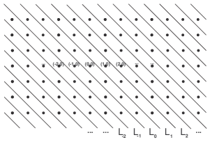
Figure 1: Slicing of the plane according to the vector $\vec{\nu}=(1,1)$.

Let us summarize the construction. We have a countable collection ${\mathcal{L}}=\{L_{i}:i\in\mathbb{Z}\}$ of lines parallel to $L_{0}$ inducing a partition of $\mathbb{Z}^{2}$. Indeed, defining $L^{*}_{i}=L_{i}\cap\mathbb{Z}^{2}$, it holds that $\mathbb{Z}^{2}=\bigcup_{i\in\mathbb{Z}}L_{i}^{*}$ (see Figure 1).

Once the plane has been sliced, any configuration $c\in A^{\mathbb{Z}^{2}}$ can be viewed as a mapping $c:\bigcup_{i\in\mathbb{Z}}L_{i}^{*}\mapsto\mathbb{Z}$. For every $i\in\mathbb{Z}$, the slice $c_{i}$ of the configuration $c$ over the line $L_{i}$ is the mapping $c_{i}:L^{*}_{i}\to A$. In other terms, $c_{i}$ is the restriction of $c$ to the set $L^{*}_{i}\subset\mathbb{Z}^{2}$. In this way, a configuration $c\in A^{\mathbb{Z}^{2}}$ can be expressed as the bi-infinite one-dimensional sequence $\prec c\succ=(\ldots,c_{-2},c_{-1},c_{0},c_{1},c_{2},\ldots)$ of its slices $c_{i}\in A^{L^{*}_{i}}$ where the $i$-th component of the sequence $\prec c\succ$ is $\prec c\succ_{i}=c_{i}$ (see Figure 2). Let us stress that each slice $c_{i}$ is defined only over the set $L^{*}_{i}$. Moreover, since $\forall\vec{x}\in\mathbb{Z}^{2},\,\exists!i\in\mathbb{Z}:\vec{x}\in L^{*}_{i}$, for any configuration $c$ and any vector $\vec{x}$ we write $c(\vec{x})=c_{i}(\vec{x})$.

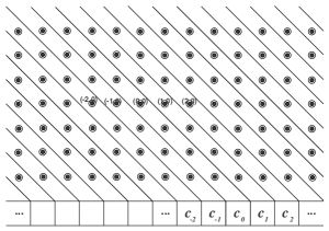
Figure 2: Slicing of a 2D configuration $c$ according to the vector $\vec{\nu}=(1,1)$. The components of $c$ viewed as a 1D configuration are not from the same alphabet.

The identification of any configuration $c\in A^{\mathbb{Z}^{2}}$ with the corresponding bi-infinite sequence of slices $c\equiv\prec c\succ=(\ldots,c_{-2},c_{-1},c_{0},c_{1},c_{2},\ldots)$, allows the introduction of a new one-dimensional bi-infinite CA over the alphabet $A^{\mathbb{Z}}$ expressed by a global transition mapping $F^{*}:(A^{\mathbb{Z}})^{\mathbb{Z}}\mapsto(A^{\mathbb{Z}})^{\mathbb{Z}}$ which associates any configuration $a:\mathbb{Z}\mapsto A^{\mathbb{Z}}$ with a new configuration $F^{*}(a):\mathbb{Z}\to A^{\mathbb{Z}}$. The local rule $f^{*}$ of this new CA we are going to define will take a certain number of configurations of $A^{\mathbb{Z}}$ as input and will produce a new configuration of $A^{\mathbb{Z}}$ as output.

For each $h\in\mathbb{Z}$, define the following bijective map $\mathcal{T}_{h}:A^{L^{*}_{h}}\mapsto A^{L^{*}_{0}}$ which associates any slice $c_{h}$ over the line $L_{h}$ with the slice $\mathcal{T}_{h}(c_{h})$

$$\left(c_{h}:L^{*}_{h}\to A\right)\quad\xrightarrow{\mathcal{T}_{h}}\quad\left(\mathcal{T}_{h}(c_{h}):L^{*}_{0}\to A\right)$$

defined as $\forall\vec{x}\in L^{*}_{0},\mathcal{T}_{h}(c_{h})(\vec{x})=c_{h}(\vec{x}+\vec{y}_{h}).$ Remark that the map $\mathcal{T}^{-1}_{h}:A^{L^{*}_{0}}\to A^{L^{*}_{h}}$ associates any slice $c_{0}$ over the line $L_{0}$ with the slice $\mathcal{T}^{-1}_{h}(c_{0})$ over the line $L_{h}$ such that $\forall\vec{x}\in L^{*}_{h},\,\mathcal{T}^{-1}_{h}(c_{h})(\vec{x})=c_{0}(\vec{x}-\vec{y}_{h})$. Denote by $\Phi_{0}:A^{L^{*}_{0}}\to A^{\mathbb{Z}}$ the bijective mapping putting in correspondence any $c_{0}:L^{*}_{0}\to A$ with the configuration $\Phi_{0}(c_{0})\in A^{\mathbb{Z}}$,

$$\left(c_{0}:L^{*}_{0}\to A\right)\quad\xrightarrow{\Phi_{0}}\quad\left(\Phi_{0}(c_{0}):\mathbb{Z}^{2}\to A\right)$$

such that $\forall t\in\mathbb{Z},\Phi_{0}(c_{0})(t):=c_{0}(\varphi^{-1}(t))$. The map $\Phi_{0}^{-1}:A^{\mathbb{Z}}\to A^{L^{*}_{0}}$ associates any configuration $a\in A^{\mathbb{Z}}$ with the configuration $\Phi^{-1}_{0}(a)\in A^{L^{*}_{0}}$ in the following way: $\forall\vec{x}\in L_{0}^{*},\,\Phi^{-1}_{0}(a)(\vec{x})=a(\varphi(\vec{x}))$. Consider now the bijective map $\Psi:A^{\mathbb{Z}^{2}}\to(A^{\mathbb{Z}})^{\mathbb{Z}}$ defined as follows

$$\forall c\in A^{\mathbb{Z}^{2}},\quad\Psi(c)=(\ldots,\Phi_{0}(\mathcal{T}_{-1}(c_{-1})),\Phi_{0}(\mathcal{T}_{0}(c_{0})),\Phi_{0}(\mathcal{T}_{1}(c_{1})),\ldots)\enspace.$$

Its inverse map $\Psi^{-1}:(A^{\mathbb{Z}})^{\mathbb{Z}}\mapsto A^{\mathbb{Z}^{2}}$ is such that $\forall a\in(A^{\mathbb{Z}})^{\mathbb{Z}}$,

$$\prec\Psi^{-1}(a)\succ=(\ldots,\mathcal{T}_{-1}^{-1}(\Phi_{0}^{-1}(a_{-1})),\mathcal{T}_{0}^{-1}(\Phi_{0}^{-1}(a_{0})),\mathcal{T}_{1}^{-1}(\Phi_{0}^{-1}(a_{1})),\ldots)\enspace.$$

Starting from a configuration $c$, the isomorphism $\Psi$ allows to obtain a 1D configuration $a$ in which all components take value from the same alphabet (see Figure 3).

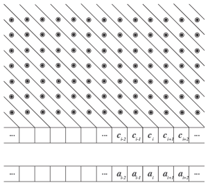
Figure 3: All the components of the 1D configuration $a=\Phi(c)$ are from the same alphabet.

At this point, we have all the necessary formalism to correctly define the radius $r^{*}$ local rule $f^{*}:(A^{\mathbb{Z}})^{2r^{*}+1}\to A^{\mathbb{Z}}$ starting from a radius $r$ 2D CA $F$. Let $r_{1}$ and $r_{2}$ be the indexes of the lines passing for $(r,r)$ and $(r,-r)$, respectively. The radius of the 1D CA is $r^{*}=\max\left\{r_{1},r_{2}\right\}$. In other words, $r^{*}$ is such that $L_{-r^{*}},\ldots L_{r^{*}}$ are all the lines which intersect the 2D $r$-radius Moore neighborhood. The local rule is defined as

$$\forall(a_{-r^{*}},\ldots,a_{r^{*}})\in(A^{\mathbb{Z}})^{2r^{*}+1},\quad f^{*}(a_{-r^{*}},\ldots,a_{r^{*}})=\Phi_{0}(b)$$

where $b:L^{*}_{0}\to A$ is the slice obtained the simultaneous application of the local rule $f$ of the original CA on the slices $c_{-r^{*}},\ldots,c_{r^{*}}$ of any configuration $c$ such that $\forall i\in[-r^{*},r^{*}],c_{i}=\mathcal{T}^{-1}_{i}(\Phi^{-1}_{0}(a_{i}))$ (see Figure 4). The global map of this new CA is $F^{*}:(A^{\mathbb{Z}})^{\mathbb{Z}}\to(A^{\mathbb{Z}})^{\mathbb{Z}}$ and the link between $F^{*}$ and $f^{*}$ is given, as usual, by

$$(F^{*}(a))_{i}=f^{*}(a_{i-r^{*}},\ldots,a_{i+r^{*}})$$

where $a=(\ldots,a_{-1},a_{0},a_{1},\ldots)\in(A^{\mathbb{Z}})^{\mathbb{Z}}$ and $i\in\mathbb{Z}$.

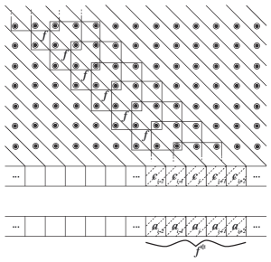
Figure 4: Local rule $f^{*}$ of the 1D CA as sliced version of the original 2D CA. Here $r=1$ and $r^{*}=2$.

The slicing construction can be summarized by the following

Theorem 3.1

Let $(A^{\mathbb{Z}^{2}},F)$ be a 2D CA and let $((A^{\mathbb{Z}})^{\mathbb{Z}},F^{*})$ be the 1D CA obtained by the $\vec{\nu}$ slicing construction of it, where $\vec{\nu}\in\mathbb{Z}^{2}$ is a fixed vector. The two CA are isomorphic by the bijective mapping $\Psi$. Moreover, the map $\Psi^{-1}$ is continuous and then $(A^{\mathbb{Z}^{2}},F)$ is a factor of $((A^{\mathbb{Z}})^{\mathbb{Z}},F^{*})$.

$$\begin{CD}(A^{\mathbb{Z}})^{\mathbb{Z}}@>{F^{*}}>{}>&(A^{\mathbb{Z}})^{\mathbb{Z}}\\ @V{\Psi^{-1}}V{}V&@V{}V{\Psi^{-1}}V\\ A^{\mathbb{Z}^{2}}@>{}>{F}>&A^{\mathbb{Z}^{2}}\end{CD}$$

Proof

It is clear that $\Psi$ is bijective. We show that $\Psi\circ F=F^{*}\circ\Psi$, i.e., that $\forall i\in\mathbb{Z},\forall c\in A^{\mathbb{Z}^{2}},\,\Psi(F(c))_{i}=F^{*}(\Psi(c))_{i}$. We have $\Psi(F(c))_{i}=\Phi_{0}(\mathcal{T}_{i}(F(c)_{i}))$ where the slice $F(c)_{i}$ is obtained by the simultaneous application of $f$ on the slices $c_{i-r^{*}},\ldots,c_{i+r^{*}}$. On the other hand $F^{*}(\Psi(c))_{i}$ is equal to

$$f^{*}(\Psi(c)_{i-r^{*}},\ldots,\Psi(c)_{i+r^{*}})=f^{*}(\Phi_{0}(\mathcal{T}_{i-r^{*}}(c_{i-r^{*}})),\ldots,\Phi_{0}(\mathcal{T}_{i+r^{*}}(c_{i+r^{*}})))=\Phi_{0}(b)$$

where, by definition of $f^{*}$, $b$ is the slice obtained by the simultaneous application of $f$ on the slices

$$d_{r^{*}}=\mathcal{T}^{-1}_{-r^{*}}(\mathcal{T}_{i-r^{*}}(c_{i-r^{*}})),\ldots,d_{r^{*}}=\mathcal{T}^{-1}_{r^{*}}(\mathcal{T}_{i+r^{*}}(c_{i+r^{*}}))$$

which gives $b=\mathcal{T}_{i}(F(c)_{i})$. We now prove that $\Psi^{-1}$ is a continuous map from the 1D CA configuration space $(A^{\mathbb{Z}})^{\mathbb{Z}}$ to the 2D CA configuration space $A^{\mathbb{Z}^{2}}$, both equipped with the corresponding metric, which for the sake of simplicity is denoted by the same symbol $d$. Choose an arbitrary configuration $a=(\ldots,a_{-1},a_{0},a_{1},\ldots)\in(A^{\mathbb{Z}})^{\mathbb{Z}}$ and a real number $\epsilon>0$. Let $n$ be a positive integer such that $\frac{1}{2^{n}}<\epsilon$. Consider the lines $L^{*}_{i}$ which intersect the 2D $n$-radius Moore neighborhood and let $m$ be the maximum of the indexes of such lines. Setting $\delta=\frac{1}{2^{m}}$, for any configuration $b\in(A^{\mathbb{Z}})^{\mathbb{Z}}$ with $d(b,a)<\delta$, we have that $b_{i}=a_{i}$ for each integer $i\in[-m,m]$. This fact implies that $(\Psi^{-1}(b))_{i}=(\Psi^{-1}(a))_{i}$ for each integer $i\in[-m,m]$, and then $(\Psi^{-1}(b))_{i}(\vec{x})=(\Psi^{-1}(a))_{i}(\vec{x})$, for each for any $\vec{x}\in L^{*}_{i}$. Equivalently, we have $(\Psi^{-1}(a))(\vec{x})=(\Psi^{-1}(b))(\vec{x})$, for any $\vec{x}\in\bigcup_{i\in[-m,m]}L^{*}_{i}$, and in particular for any $\vec{x}$ such that $|\vec{x}|\leq n$. Hence, $d(\Psi^{-1}(b),\Psi^{-1}(a))<\epsilon$ and $\Psi^{-1}$ is continuous.

Remark 1

The above constructions do not depend neither on the norm nor on the sense of the vector $\vec{\nu}$. In other words, if $\vec{\nu}$ is a normalized vector, all $k\vec{\nu}$–slicing ($k\in\mathbb{Z}$) constructions of a CA $F$ generate the same CA $F^{*}$.

3.1 $\vec{\nu}$-Slicing with finite alphabet

Fix a vector $\vec{\nu}\in\mathbb{Z}^{2}$. For any 2D CA $F$, we can build an associated sliced version $F^{*}$ with finite alphabet by considering the $\vec{\nu}$-slicing construction of the 2D CA restricted on the set $S_{\vec{v}}$, where $\vec{v}$ is any vector such that $\vec{v}\perp\vec{\nu}$. This is possible since the set $S_{\vec{v}}$ is $F$-invariant and so $(S_{\vec{v}},F)$ is a DTDS. The obtained construction leads to the following

Theorem 3.2

Let $F$ be a 2D CA and $\vec{\nu}\in\mathbb{Z}^{2}$. For any vector $\vec{v}\in\mathbb{Z}^{2}$ with $\vec{v}\perp\vec{\nu}$, the DTDS $(S_{\vec{v}},F)$ is topologically conjugated to the 1D CA $(B^{\mathbb{Z}},F^{*})$ on the finite alphabet $B=A^{|\vec{v}|}$ obtained by the $\vec{\nu}$–slicing construction of $F$ restricted on $S_{\vec{v}}$.

$$\begin{CD}B^{\mathbb{Z}}@>{F^{*}}>{}>&B^{\mathbb{Z}}\\ @V{\Psi^{-1}}V{}V&@V{}V{\Psi^{-1}}V\\ S_{\vec{v}}@>{}>{F}>&S_{\vec{v}}\end{CD}$$

Proof

Fix a vector $\vec{v}\perp\vec{\nu}$. Consider the slicing construction on $S_{\vec{v}}$. According to it, any configuration $c\in S_{\vec{v}}$ is identified with the corresponding bi-infinite sequence of slices. Since slices of configurations in $S_{\vec{v}}$ are in one-to-one correspondence with symbols of the alphabet $B$, the $\vec{\nu}$–slicing construction gives a 1D CA $F^{*}:B^{\mathbb{Z}}\to B^{\mathbb{Z}}$ such that, by Theorem 3.1, $(S_{\vec{v}},F)$ is isomorphic to $(B^{\mathbb{Z}},F^{*})$ by the bijective map $\Psi:S_{\vec{v}}\to B^{\mathbb{Z}}$. By Theorem 3.1, $\Psi^{-1}$ is continuous. Since configurations of $S_{\vec{v}}$ are periodic with respect to $\sigma^{\vec{v}}$, $\Psi$ is continuous too.

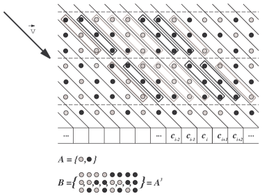
Figure 5: $\vec{\nu}$–slicing of a configuration $c\in S_{\vec{v}}$ on the binary alphabet $A$ where $\vec{\nu}=(1,1)$ and $\vec{v}=(3,-3)$. The configuration $\Psi(c)$ is on the alphabet $B=A^{3}$.

The previous result is very useful since one can use all the well-known results about 1D CA and try to lift them to $F$.

4 Closingness and Openness for 2D CA.

The notion of closingness is of interest in 1D symbolic dynamics since it is tightly linked to several and important dynamical behaviors. Moreover, it is a decidable property. In this section, we generalize the definition of closingness to any direction and we prove a strong relation w.r.t. openness.

Notation.

For any $\vec{\nu}\in\mathbb{Z}^{2}$, define $\bar{\vec{\nu}}=-\vec{\nu}$.

Definition 1 ($\vec{\nu}$-asymptotic configurations)

Two configurations $c,c^{\prime}\in A^{\mathbb{Z}^{2}}$ are $\vec{\nu}$-asymptotic if there exists $q\in\mathbb{Z}$ such that $\forall\vec{x}\in\mathbb{Z}^{2}$ with $\vec{\nu}\cdot\vec{x}\geq q$ it holds that $c(\vec{x})=c^{\prime}(\vec{x})$.

Definition 2 ($\vec{\nu}$-closingness)

A 2D CA $F$ is $\vec{\nu}$-closing if for any pair of $\bar{\vec{\nu}}$-asymptotic configurations $c,c^{\prime}\in A^{\mathbb{Z}^{2}}$ we have that $c\neq c^{\prime}$ implies $F(c)\neq F(c^{\prime})$. A 2D CA is closing if it is $\vec{\nu}$-closing for some $\vec{\nu}$.

Definition 3 ($\vec{\nu}$-$\vec{\mu}$-closingness)

A 2D CA $F$ is $\vec{\nu}$-$\vec{\mu}$-closing if for any pair of $\bar{\vec{\nu}}$-$\bar{\vec{\mu}}$-asymptotic configurations (i.e. configurations which are both $\bar{\vec{\nu}}$-asymptotic and $\bar{\vec{\mu}}$-asymptotic) $c,c^{\prime}\in A^{\mathbb{Z}^{2}}$, we have that $c\neq c^{\prime}$ implies $F(c)\neq F(c^{\prime})$.

Thanks to the $\vec{\nu}$-slicing construction with finite alphabet, the following properties hold.

Proposition 1 ([dennunzio08, dennunzio09ja])

Let $F$ be a $\vec{\nu}$-closing 2D CA. For any vector $\vec{v}\in\mathbb{Z}^{2}$ with $\vec{v}\perp\vec{\nu}$, let $(B^{\mathbb{Z}},F^{*})$ be the 1D CA of Theorem 3.2 which is topologically conjugated to $(S_{\vec{v}},F)$. Then $F^{*}$ is either right or left closing.

Theorem 4.1 ([dennunzio08, dennunzio09ja])

Any closing 2D CA has DPO.

Recall that a pattern $P$ is a function from a finite domain $Dom(P)\subseteq\mathbb{Z}^{2}$ taking values in $A$. The notion of cylinder can be conveniently extended to general patterns as follows: for any pattern $P$, let $[P]$ be the set

$$\left\{c\in A^{\mathbb{Z}^{2}}\;|\;\forall\vec{x}\in Dom(P),c(\vec{x})=P(\vec{x})\right\}\enspace.$$

As in the 1D case, cylinders form a basis for the open sets. For $h,t\geq 1$ and any normalized vectors $\vec{\nu},\vec{\mu}\in\mathbb{Z}^{2}$, we say that a pattern $u$ has a $(\vec{\nu},\vec{\mu})$–shape of size $\mathbf{[}h,t\mathbf{]}$ if for some $q,q^{\prime}\in\mathbb{Z}$ it holds that

$$dom(u)=\left\{\vec{x}\in\mathbb{Z}^{2}\;|\;q\leq\vec{\nu}\vec{x}<q+h\;\text{and}\;q^{\prime}\leq\vec{\mu}\vec{x}<q^{\prime}+t\right\}\enspace.$$

The following result is an improvement of [dennunzio08, Thm. 2] and gives a tight relation between closingness and openess.

Theorem 4.2

If a 2D CA $F$ is both $\vec{\nu}$ and $\bar{\vec{\nu}}$–closing, then it is open.

Proof

We show that the image of any cylinder with $(\vec{\nu},\vec{\mu})$ shape is open, where $\vec{\mu}\perp\vec{\nu}$. Fix a cylinder $[u]$ where $u$ is a pattern centered in the origin and having a $(\vec{\nu},\vec{\mu})$–shape of size $\mathbf{[}2h+1,2t+1\mathbf{]}$. Let $\vec{k}\perp\vec{\nu}$ with $|\vec{k}|=2t+1$ and denote $S^{\prime}_{n}=S_{n\vec{k}}$. Consider the dense set $S=\bigcup_{n\in\mathbb{N}}S^{\prime}_{n}$ endowed with the relative topology ${\mathcal{R}}$.

First of all, we prove that $F([u]\cap S)$ is open in ${\mathcal{R}}$. Choose a cylinder $[v]$ where $v$ is a pattern centered in the origin and having a $(\vec{\nu},\vec{\mu})$–shape of size $\mathbf{[}2l+1,2t+1\mathbf{]}$ with $l>h$. In the sequel, we show that any configuration from $[v]\cap S$ has a pre-image in $[u]$. If $c\in[v]\cap S$ there exists $n$ such that $c\in S^{\prime}_{n}\cap[v^{\prime}]$ where $[v^{\prime}]\subset[v]$ is the cylinder individuated by a pattern $v^{\prime}$ having a $(\vec{\nu},\vec{\mu})$–shape of size $\mathbf{[}2l+1,s\mathbf{]}$ with $s=n|\vec{v}|\geq 2t+1$. Let $(B^{\mathbb{Z}},F^{*})$ be the 1D CA which is topologically conjugated to $(S^{\prime}_{n},F)$. By hypothesis and the slicing construction, $(B^{\mathbb{Z}},F^{*})$ is both left and right closing. Let $m>0$ be a integer from [kurka04, Prop. 5.44]. Thus there is a cylinder $[w]\subset[v^{\prime}]\subset[v]$ individuated by a pattern $w$ having a $(\vec{\nu},\vec{\mu})$–shape of size $\mathbf{[}2m+1,s\mathbf{]}$ and such that $c\in[w]$. Equivalently, $\Psi(c)$ belongs to the 1D cylinder $[\bar{w}]=\Psi([w]\cap S^{\prime}_{n})\subset B^{\mathbb{Z}}$. Using [kurka04, Prop. 5.44] and a completeness argument, we obtain that $\Psi(c)$ has a preimage in the 1D cylinder $[\bar{u}]=\Psi([u]\cap S^{\prime}_{n})\subset B^{\mathbb{Z}}$. This means that $c$ has a preimage in $[u]$. Therefore, for a fixed integer $l>h$,

$$F([u]\cap S)=\bigcup\left\{[v]:F([u])\cap[v]\neq\emptyset,\;\text{and $v$ has $(\vec{\nu},\vec{\mu})$ shape of size}\;\mathbf{[}2l+1,2t+1\mathbf{]}\right\}$$

is a union of cylinders and hence $F([u]\cap S)$ is open in ${\mathcal{R}}$.

It remains to prove that $F$ is open in the whole topology on $A^{\mathbb{Z}^{2}}$. Let $[u]$ be a cylinder and $c\in F([u])$. Since $S$ is dense in $F([u])$, for any $r>0$ the ball $\mathcal{B}_{r}(c)$ of center $c$ and radius $r$ contains a configuration $c^{\prime}\in S$. In particular $\mathcal{B}_{r}(c)=\mathcal{B}_{r}(c^{\prime})$. Since $F$ is open in the relative topology $\mathcal{R}$, there exists $\mathcal{B}_{r}(c^{\prime})\cap S\subset F[u]\cap S$. Let $b\in\mathcal{B}_{r}(c^{\prime})$. Since $S$ is dense, there is a sequence $\{b^{(n)}\}\in\mathcal{B}_{r}(c^{\prime})\cap F([u])\cap S$ converging to $b$. Since $F([u])$ is closed, then $b\in F([u])$. Thus, $\mathcal{B}_{r}(c^{\prime})\subset F([u])$. ∎

Proposition 2 ([dennunzio08, dennunzio09ja])

Any open 2D CA is surjective.

5 Quasi-expansivity

Shereshevsky proved that there are no positively expansive 2D CA [shereshevsky93]. Nevertheless, when watching the evolution of some 2D CA on a computer display, one can see many similarities with positively expansive 1D CA. Given two configurations, call defect any difference between them. Intuitively, a positively expansive CA is able to produce new defects at each evolution step and spread them to any direction of the cellular space. If in the 1D case, this is possible since there are only two directions (left and right), this is not the case for CA over a 2D lattice where the number of possible directions is infinite. In this section we introduce the notion of quasi-expansivity and we show that it shares with positive expansivity many of the features just discussed.

Definition 4 (Quasi–Expansivity)

A 2D CA $F$ is $\vec{\nu}$–expansive if the 1D CA $((A^{\mathbb{Z}})^{\mathbb{Z}},F^{*})$ obtained by the $\vec{\nu}$-slicing of it is positively expansive. A 2D CA $F$ is quasi–expansive if it is $\vec{\nu}$-expansive for some $\vec{\nu}\in\mathbb{Z}^{2}$.

The following result follows from definition 4 and it will be useful in the sequel.

Lemma 1

Let $F$ be a $\vec{\nu}$–expansive 2D CA. For any vector $\vec{v}\in\mathbb{Z}^{2}$ with $\vec{v}\perp\vec{\nu}$, let $(B^{\mathbb{Z}},F^{*})$ be the 1D CA of Theorem 3.2 which is topologically conjugated to $(S_{\vec{v}},F)$. Then $F^{*}$ is positively expansive.

Theorem 5.1

Any $\vec{\nu}$–expansive 2D CA is both $\vec{\nu}$ and $\bar{\vec{\nu}}$–closing.

Proof

Suppose that $F$ is not $\vec{\nu}$–closing. Then, there exist two distinct $\bar{\vec{\nu}}$–asymptotic configurations $c,c^{\prime}$ such that $F(c)=F(c^{\prime})$. Let $\varepsilon$ be the expansivity constant of the $\vec{\nu}$–sliced CA $F^{*}$. By a shift argument, we can assume that $d(\Psi(c),\Psi(c^{\prime}))<\varepsilon$. Thus, for any $t\in\mathbb{N}$ it holds that $d(F^{*t}(\Psi(c)),F^{*t}(\Psi(c^{\prime})))<\varepsilon$. The proof for $\bar{\vec{\nu}}$–closingness is similar.∎

Corollary 1

Any quasi–expansive 2D CA has DPO, it is surjective and open.

Proof

It is an immediate consequence of Theorems 4.1, 4.2 and 5.1.∎

Theorem 5.2

Any quasi–expansive 2D CA $F$ is topologically mixing.

Proof

Assume that $F$ is $\vec{\nu}$–expansive. Choose $\varepsilon>0$ and $c,c^{\prime}\in A^{\mathbb{Z}^{2}}$. Take $\vec{v}\in\mathbb{Z}^{2}$ with $\vec{v}\perp\vec{\nu}$ and $e,e^{\prime}\in S_{\vec{v}}$ such that $d(c,e)<\varepsilon$ and $d(c^{\prime},e^{\prime})<\varepsilon$. Since $F$ is $\vec{\nu}$–expansive, by Lemma 1, $(S_{\vec{v}},F)$ topologically conjugated to a 1D CA $(B^{\mathbb{Z}},F^{*})$ where $F^{*}$ is positively expansive and $B$ is finite. Since positively expansive 1D CA on a finite alphabet are topologically mixing [kurka97, blanchard97], there exist a sequence $\{b^{(n)}\}\subset S_{\vec{v}}$ and an integer $m\geq 0$ such that for all $n\geq m$ it holds that $d(b^{(n-m)},e)<\varepsilon$ and $d(F^{n}(b^{(n-m)}),e^{\prime})<\varepsilon$. This concludes the proof.∎

Let $\vec{\gamma}\in\{(1,1),(-1,1),(-1,-1),(1,-1)\}$. We now give an example of a class of 2D CA which are quasi-expansive.

Definition 5 (Permutivity)

A 2D CA of local rule $f$ and radius $r$ is $\vec{\gamma}$-permutive, if for each pair of matrices $N,N^{\prime}\in\mathcal{M}_{r}$ with $N(\vec{x})=N^{\prime}(\vec{x})$ in all vectors $\vec{x}\neq r\vec{\gamma}$, it holds that $N(r\vec{\gamma})\neq N^{\prime}(r\vec{\gamma})$ implies $f(N)\neq f(N^{\prime})$. A 2D CA is bi-permutive iff it is both $\vec{\gamma}$ permutive and $\bar{\vec{\gamma}}$-permutive.

The previous definition is given assuming a $r$ radius Moore neighborhood. It is not difficult to generalize it to suitable neighborhoods. The proofs of the results concerning permutivity with different neighborhood can also be adapted.

Proposition 3 ([dennunzio08, dennunzio09ja])

Consider a $\vec{\gamma}$-permutive 2D CA $F$. For any $\vec{\nu}$ belonging either to the same quadrant or the opposite one as $\vec{\gamma}$, the 1D CA $((A^{\mathbb{Z}})^{\mathbb{Z}},F^{*})$ obtained by the $\vec{\nu}$-slicing construction is either rightmost or leftmost permutive.

Lemma 2

Let $(A^{\mathbb{Z}},F)$ be a 1D CA on a possibly infinite alphabet $A$. If $F$ is both leftmost and rightmost permutive, then $F$ is positively expansive.

Proof

We show that $F$ is positively expansive with constant $\varepsilon=2^{-r}$ where $r$ is the radius of the CA. Choose $c,c^{\prime}\in A^{\mathbb{Z}}$ with $c\neq c^{\prime}$ and assume that for all $t\in\mathbb{N}$, $F^{t}(c)_{[-r,r]}=F^{t}(c^{\prime})_{[-r,r]}$. Suppose that $c_{i}\neq c^{\prime}_{i}$ with $i>r$. Let $n=\lfloor i/r\rfloor$ and $q=i-nr\in[0,r)$. Since $F^{n}$ is rightmost permutive and $F^{n}(c)_{q}=F^{n}(c^{\prime})_{q}$ then $c_{i}=c^{\prime}_{i}$. The case $c_{i}\neq c^{\prime}_{i}$ with $i<-r$ is similar.∎

Proposition 4

A 2D CA $F$ which is both $\vec{\gamma}$ and $\bar{\vec{\gamma}}$–permutive is $\vec{\nu}$-expansive for any $\vec{\nu}$ belonging either to the same quadrant or the opposite one as $\vec{\gamma}$.

Proof

By Proposition 3, for any $\vec{\nu}$ like in the hypothesis, the 1D CA $((A^{\mathbb{Z}})^{\mathbb{Z}},F^{*})$ obtained by the $\vec{\nu}$-slicing construction is both rightmost and leftmost permutive. By Lemma 2, $((A^{\mathbb{Z}})^{\mathbb{Z}},F^{*})$ is positively expansive and then $F$ is $\vec{\nu}$–expansive.∎

Remark that a 2D CA can be $\vec{\nu}$-expansive for a certain direction $\vec{\nu}$ but not for other directions as illustrated by the following example.

Example 1

Consider the 2D CA $F$ of radius $1$ on the binary alphabet which local rule performs the xor operation on the two corners $\vec{\gamma}=(1,1)$ and $\bar{\vec{\gamma}}=(-1,-1)$ of the Moore neighborhood. Since $F$ is both $\vec{\gamma}$ and $\bar{\vec{\gamma}}$–permutive, $F$ is $\vec{\nu}$–expansive, and then $\vec{\nu}$–closing, for all $\vec{\nu}$belonging either to the same quadrant or the opposite one as $\vec{\gamma}$. On the other hand, for $\vec{\nu}=(1,-1)$ or $\vec{\nu}=(-1,1)$, $F$ is not $\vec{\nu}$–closing and then not $\vec{\nu}$-expansive.∎

Proposition 5

Any bipermutive 2D CA $F$ is open.

Proof

If $F$ is both $\vec{\gamma}$ and $\bar{\vec{\gamma}}$–permutive then, by [dennunzio08, Prop. 5], it is both $\vec{\gamma}$ and $\bar{\vec{\gamma}}$–closing. Theorem 4.2 concludes the proof.∎

5.1 Topological entropy of quasi-expansive CA

The topological entropy is generally accepted as a measure of the complexity of a DTDS. The problem of computing (or even approximating) it for CA is algorithmically unsolvable [hurd92]. However, in [damico03], the authors provided a closed formula for computing the entropy of two important classes, namely additive CA and positively expansive CA. In particular, they proved that for the first class, the entropy is either $0$ or $\infty$. Furthermore, in [mey08], multidimensional cellular automata with finite nonzero entropy are exhibited. In this section, we shall see another example of important class of CA with infinite topological entropy.

Notation.

Given a 1D CA F and $w,t\in\mathbb{N}$, let $N_{F}(w,t)$ be the number of distinct rectangles of width $w$ and height $t$ occurring in all possible space-time diagrams of $F$. Similarly, if $F$ is a D-dimensional CA, $N_{F}(w^{(D)},t)$ is the number of distinct $D+1$ dimensional hyper-rectangles of height $t$ and basis $w^{(D)}$, where $w^{(D)}$ is the $D$-dimensional hypercube of sides $w$.

In the case of D-dimensional CA, the definition of topological entropy for DTDS simplifies as follows [hurd92, damico03]:

$$H(A^{\mathbb{Z}^{D}},F)=\lim_{w\to\infty}\lim_{t\to\infty}\frac{\log N_{F}(w^{(D)},t)}{t}\enspace.$$

For introductory matters about topological entropy see [kurka04].

Theorem 5.3

Any quasi-expansive 2D (or higher) CA has infinite topological entropy.

Proof

Consider a $\vec{\nu}$–expansive 2D CA (for higher dimensions the proof is similar). Fix a vector $\vec{v}\in\mathbb{Z}^{2}$ with $\vec{v}\perp\vec{\nu}$. For any $n\in\mathbb{N}$, let $S^{\prime}_{n}=S_{2^{n}\cdot\vec{v}}$. By Lemma 1 and Theorem 3.2, any DTDS $(S^{\prime}_{n},F)$ is topologically conjugated to a positively expansive 1D CA on a finite alphabet. By [nasu95, Thm. 3.12], each $(S^{\prime}_{n},F)$ is also topologically conjugated to the DTDS $((C_{n})^{\mathbb{N}},\sigma)$ for a suitable finite alphabet $C_{n}$. Thus, for any $n\in\mathbb{N}$, $H(S^{\prime}_{n},F)=\log|C_{n}|$ where $|C_{n}|$ also represents the number of preimages of any element of $S^{\prime}_{n}$. Since $S^{\prime}_{n}\subset S^{\prime}_{n+1}$, it holds that $H(S^{\prime}_{n},F)\leq H(S^{\prime}_{n+1},F)$. We show that $H(S^{\prime}_{n},F)<H(S^{\prime}_{n+1},F)$ for any $n\in\mathbb{N}$. This permits to conclude the proof since $H(S^{\prime}_{n},F)\leq H(A^{\mathbb{Z}^{2}},F)$ for all $n\in\mathbb{N}$.

For the sake of argument, assume that $H(S^{\prime}_{n},F)=H(S^{\prime}_{n+1},F)$ for some $n\in\mathbb{N}$. Thus, any element in $S^{\prime}_{n}$ has exactly $k$ pre–images in $S^{\prime}_{n}$ and any element in $S^{\prime}_{n+1}$ has exactly $k$ pre–images in $S^{\prime}_{n+1}$, where $k=|C_{n}|=|C_{n+1}|$. As a consequence, it holds that $F(S^{\prime}_{n+1}\setminus S^{\prime}_{n})\subseteq S^{\prime}_{n+1}\setminus S^{\prime}_{n}$. Since $(S^{\prime}_{n+1},F)$ is topologically conjugated to $((C_{n+1})^{\mathbb{N}},\sigma)$, it is also strongly transitive. Thus, if $c$ is any configuration in $S^{\prime}_{n}$ and $[u]$ is any 1D cylinder in $S^{\prime}_{n+1}\setminus S^{\prime}_{n}$, then $F(d)=c$ for some $d\in S^{\prime}_{n+1}\setminus S^{\prime}_{n}$ and $t\in\mathbb{N}$. Therefore $F(S^{\prime}_{n+1}\setminus S^{\prime}_{n})\cap S^{\prime}_{n}\neq\emptyset$ and this is a contradiction. ∎

6 Quasi-almost equicontinuity vs. quasi-sensitivity

In a similar way as quasi-expansivity, one can define quasi-sensitivity and quasi-almost-equicontinuity.

Definition 6 (Quasi-almost equicontinuity)

A 2D CA $F$ is $\vec{\nu}$–almost equicontinuos if the 1D CA $((A^{\mathbb{Z}})^{\mathbb{Z}},F^{*})$ obtained by the $\vec{\nu}$ slicing of it is almost equicontinuous. A 2D CA $F$ is quasi-almost equicontinuous if it is $\vec{\nu}$–almost equicontinuous for some $\vec{\nu}\in\mathbb{Z}^{2}$.

Definition 7 (Quasi-sensitivity)

A 2D CA $F$ is $\vec{\nu}$–sensitive if the 1D CA $((A^{\mathbb{Z}})^{\mathbb{Z}},F^{*})$ obtained by the $\vec{\nu}$ slicing of it is sensitive. A 2D CA $F$ is quasi-sensitive if it is $\vec{\nu}$–sensitive for some $\vec{\nu}\in\mathbb{Z}^{2}$.

Proposition 6

Any 2D CA $F$ is $\vec{\nu}$-almost equicontinuous iff it is not $\vec{\nu}$-sensitive.