On The Critical Packet Injection Rate Of A Preferential Next-Nearest Neighbor Routing Traffic Model On Barabási-Albert Networks

Abstract

Recently, Yin et al. [Eur. Phys. J. B 49, 205 (2006)] introduced an efficient small-world network traffic model using preferential next-nearest neighbor routing strategy with the so-called path iteration avoidance (PIA) rule to study the jamming transition of internet. Here we study their model without PIA rule by a mean-field analysis which carefully divides the message packets into two types. Then, we argue that our mean-field analysis is also applicable in the presence of PIA rule in the limit of a large number of nodes in the network. Our analysis gives an explicit expression of the critical packet injection rate $R_{c}$ as a function of a bias parameter of the routing strategy $\alpha$ in their model with or without PIA rule. In particular, we predict a sudden change in $R_{c}$ at a certain value of $\alpha$. These predictions agree quite well with our extensive computer simulations.

I Introduction

Complex networks with small-world property exist in many natural and social systems, such as food web, the internet Pastor-Satorras et al. (2001); Vázquez et al. (2002), the world wide web Albert et al. (1999), and the world-wide airport network (WAN) Guimerà et al. (2005). In 1999, Barabási and Albert proposed a scale-free growing model (BA network) with a preferential attachment mechanism to mimic a growing small-world network in the real world Barabási and Albert (1999). Their model stimulated the interest of the physics community to study complex networks by statistical physical means Albert and Barabási (2002); Newman (2003). One of the goals of these studies is to understand the dynamical processes taking place behind the underlying structure.

It is instructive to study the traffic capacity of a network. We may start by considering the simple-minded situation in which message packets are injected randomly into the nodes of the network at a fixed rate. Each packet has a randomly assigned destination node. And each node in the network has a finite message-forwarding rate. Clearly, an important factor affecting network traffic capacity is the routing strategy, namely, how each node forwards its out-going message packets to its nearest neighbors. The performance indicator is the maximum free-flowing traffic capacity characterized by the critical packet generation rate $R_{c}$. More precisely, $R_{c}$ is the supremum number of new packets that can be injected into the network per unit time step without causing congestion de Menezes and Barabási (2004); Germano and de Moura (2006). Here, congestion means that the average rate of change of the number of packets in some node is positive. (Actually, this performance indicator is not overly stringent for the model investigated in this paper as we find that the number of packet in almost all nodes steadily increases over time without saturation whenever $R>R_{c}$.) The more efficient the routing strategy, the larger the value of $R_{c}$. For a sufficiently large random network, the routing strategy cannot depend on the network topology because this information is not available to each node. Thus, it is reasonable to confine ourselves to study local routing strategies.

Perhaps the simplest local routing strategies are the ones that use information on the nearest neighbors of individual node Adamic et al. (2001); Tadić et al. (2004). Recently, based on these nearest-neighbors-based strategies, a new routing strategy called the preferential next-nearest-neighbor (PNNN) searching strategy was proposed by Yin et al. Yin et al. (2006) in which the performance is better than those using nearest neighbor routing. As the name suggests, in PNNN, a message packet looks for its destination among the next nearest neighbors of the node it currently stays. If the destination cannot be found in this way, the message packet will be forwarded to a neighboring node by a biased random walk with a preferential probability which depends on a parameter called preferential delivering exponent $\alpha$. To speed up packet delivery, Yin et al. added in their routing strategy the path iteration avoidance (PIA) rule, which states that a packet cannot travel through an edge more than twice.

As a model of scale-free network traffic with potential applications in the internet and the world wide web, the use of PIA rule is problematic. A message packet, unlike a human driver, cannot automatically remember the path it has traveled. This additional piece of information, whose length grows linearly with the time since creation of the packet, may either be stored in, say, a central registry, or attached to the message packet itself. Thus, the cost of inquiring this information from the registry or transmitting it through an edge alongside with the message packet cannot be ignored. Furthermore, additional computational cost, which also scales linearly with the time since the creation of the packet, is needed for a node to process this historical path information in accordance with the PIA rule. All these factors make the effective message packet forwarding rate a function of the time since the packet creation. Unfortunately, the PNNN routing strategy of Yin et al. Yin et al. (2006) does not take these extra communication and computational costs into account. This is why we believe that PIA rule is not very realistic.

In Sec. II, we briefly review the network traffic model proposed by Yin et al. Yin et al. (2006) using the PNNN strategy. Then we perform mean-field analytical calculation for the dynamics of their model with and without the PIA rule in Sec. III. In both cases, we find an abrupt change in the dependence of $R_{c}$ on $\alpha$ at certain value of $\alpha$. We also give the physical reason behind such change. In Sec. IV, we compare the mean-field calculations with our extensive numerical simulation results of $R_{c}$ against $\alpha$. We also show in this Section that the network size used in Yin et al.’s numerical simulations is not large enough to reveal the thermodynamic behavior of their model. Finally, we give a brief summary and discuss the effectiveness of the PNNN strategy in Sec. V.

II The PNNN+PIA And PNNN-PIA Models

Yin et al. proposed and studied the following network traffic model on a BA network Yin et al. (2006). (Here we call their model with and without the PIA rule PNNN+PIA and PNNN-PIA, respectively.) Their model consists of a random but fixed BA network with $N$ nodes. We denote the set of all nodes in this network by ${\mathbb{V}}$. We further denote the degree of the node having the least (greatest) number of nearest neighbors in the network by $k_{\min}$ ($k_{\max}$). That is to say,

$$k_{\min}\equiv\min_{i\in{\mathbb{V}}}k_{i}$$ (1)

and

$$k_{\max}\equiv\max_{i\in{\mathbb{V}}}k_{i},$$ (2)

where $k_{i}$ is the degree of the node $i$. Recall that BA network is generated by connecting each newly added node to $m$ existing nodes in a careful way Barabási and Albert (1999). Hence,

$$k_{\min}=m.$$ (3)

Further recall that during the generation of a BA network, the average degree of the node added to the network $t_{\text{elapse}}$ ago equals $m(N/t_{\text{elapse}})^{1/2}$ Barabási and Albert (1999). Thus,

$$k_{\max}\approx m\sqrt{N}.$$ (4)

We denote the adjacency matrix of the network by $A$. That is, $A_{ij}=1(0)$ if there is an (no) edge between nodes $i$ and $j$.

In PNNN+PIA and PNNN-PIA, each node has an unlimited buffer, known as load, to store packets. At each time step, each of the $R$ packets is added to a randomly chosen source node of the network with a randomly chosen destination node. Note that simulations reported by Yin et al. in Ref. Yin et al. (2006) were performed by considering only integer values of $R$. In contrast, we allow a real-valued $R$. More precisely, we inject a message packet into a node with probability $R/N$ in each time step.

Each node can send out at most $C\geq 1$ packets to its nearest neighbors using the first-in-first-out rule. That is to say, packets entering a node first will be sent out first. Each out-going packet first searches through all the next nearest neighbors of the node to which it currently belongs. If its destination is located in this search, the packet will be forwarded to one of the neighbors connecting the destination and the current node. And in the next time step, this packet will be forwarded to the destination and then removed from the network. If the destination of an out-going message packet cannot be found in such a search, it will be randomly forwarded from its current node (say, node $i$) to one of the neighbors (say, node $j$) with probability

$$\Pi_{ij}=\frac{k_{j}^{\alpha}}{\sum_{\ell\in{\mathbb{V}}}A_{i\ell}k_{\ell}^{\alpha}},$$ (5)

where $\alpha$ is a fixed parameter known as the preferential delivering exponent. Note that the sum in the above equation can be regarded as a restricted sum over the nearest neighbors of the packet’s current node $i$.

The only difference between PNNN+PIA and PNNN-PIA is that PIA rule is present in the former model while absent in the latter. Recall that PIA rule demands each packet to travel through the same edge at most twice Yin et al. (2006). In the event that a message packet has nowhere to go due to the PIA rule, the packet will be removed from the network. And for $\alpha\in[-4,2]$, only a very small percentage of packets are removed from the network in this way Wang et al. (2008).

Clearly, historical path information of a packet is needed to decide where it will go in the next time step with the adoption of PIA rule. As we have mentioned in Sec. I, extra communication and processing costs are required to forward a message packet together with its historical path information in the network to its neighboring node. Thus, it is less efficient to forward an old packet than a newly created one. In this respect, PIA rule is not consistent with the rule that the message forwarding capability of a node is independent of the age of the forwarding packets. This is a serious problem because Yin et al. found by numerical simulation that the packet lifetime, which is the time between its injection and removal, roughly obeys a power law distribution Yin et al. (2006).

Although Yin et al. has briefly studied the PNNN-PIA model numerically in Ref. Yin et al. (2006), their focus was on the PNNN+PIA model. They found that the critical packet generation rate $R_{c}$ is increased by adopting the PIA rule. More importantly, using numerical simulation up to $N\approx 5000$ with $R$ restricted to integers only, they found that $R_{c}$ is a decreasing function of $\alpha$ for the PNNN+PIA model. In addition, based on their simulations in the range $\alpha\in[-4,2]$, they believed that for a fixed $N$, the value of $R_{c}$ is a constant whenever $\alpha\leq-2$ Yin et al. (2006).

An interesting common feature of the PNNN+PIA and PNNN-PIA models is that as long as there are no more than $C$ message packets staying in a node at any time, the message packets behave like independent particles in the sense that their motions in the BA network are independent of each other. This property is important in our subsequent discussions.

III Mean-field Analysis

III.1 The PNNN-PIA Model

We try to calculate the $R_{c}$ against $\alpha$ curve for the PNNN-PIA model by mean-field approximation. The validity of the approximations made in our calculation will be discussed and justified in Sec. IV. Let us begin by classifying the packets into two types. A packet is called a destination located packet (DLP) if it has successfully found a path to its destination. By the rules of PNNN-PIA, the destination of a DLP must be one of the nearest or next nearest neighboring nodes of its current location. Otherwise, the packet is known as a destination seeking packet (DSP). Since a newly injected packet has not found out its path to the destination yet, it must a DSP. A DSP moves randomly to its neighboring node with probability given by Eq. (5). We denote the numbers of DLPs and DSPs in node $i$ at time $t$ by $n_{l,i}(t)$ and $n_{s,i}(t)$, respectively.

We say that a network is in free-flow state if each node, on average, can forward all its loads in the next time step. (In other words, the average load of each node is at most $C$ in each time step.) In this case, node $i$ can, on average, send out all its $n_{s,i}(t)$ message packets at any time $t$. At the same time, node $i$ receives, on average, $R/N$ DSPs by packet generation. Since the number of 4-cycles in a BA network scales like $\left[m\log(N)/2\right]^{4}/4$ Bianconi (2004), the probability that two next nearest neighboring nodes are connected to more than one common node goes to 0 in the large $N$ limit. So the number of next nearest neighbors for node $i$ is approximately equal to $\sum_{j\in{\mathbb{V}}}A_{ij}(k_{j}-1)$ in the large $N$ limit. Consider a DSP that reaches the node $i$ for the first time. Then, the probability $\Phi_{i}$ that it can locate a path to its destination in the next time step is given by

$$\Phi_{i}\approx\frac{1}{N}\sum_{j\in{\mathbb{V}}}A_{ij}(k_{j}-1).$$ (6)

In contrast, suppose the DSP has reached the node $i$ more than once, then it has no chance to find the path to its destination in the next time step as the next nearest neighbors of node $i$ has been searched during its previous visit to node $i$. Let $\lambda_{j}$ be the average number of visit of a DSP to node $j$ given that it has visited node $j$ at least once. Then, using the mean-field approximation similar to that used in Ref. Wang et al. (2006), the number of DSP in free-flow state satisfies

$$\frac{dn_{s,i}(t)}{dt}\approx\frac{R}{N}-n_{s,i}(t)+\sum_{j\in{\mathbb{V}}}A_{ij}n_{s,j}(t)\Pi_{ji}\left(1-\frac{\Phi_{j}}{\lambda_{j}}\right).$$ (7)

Note that $1-\Phi_{j}/\lambda_{j}$ is the probability that a DSP at node $j$ will not change to a DSP in the next time step. Thus, the last term in the R.H.S. of the above equation is the average number of DSPs received by node $i$ from its neighbors.

We want to study the equilibrated distribution of DSPs for a typical node in the free-flow state as a function of the degree of the node. And we do so by investigating

$$n_{s}(k)\equiv\frac{\left\langle\sum_{i\in{\mathbb{V}}}\delta_{k_{i},k}n_{s,i}(t)\right\rangle_{t}}{\sum_{i\in{\mathbb{V}}}\delta_{k_{i},k}},$$ (8)

where $\delta_{k_{i},k}$ is the Kronecker delta and $\left\langle\cdots\right\rangle_{t}$ represents the time average of its argument. Upon equilibration,

$$\left\langle n_{s,i}(t)\right\rangle_{t}\approx\frac{R}{N}+\sum_{j\in{\mathbb{V}}}A_{ij}\left\langle n_{s,j}(t)\right\rangle_{t}\Pi_{ji}\left(1-\frac{\Phi_{j}}{\lambda_{j}}\right).$$ (9)

Although BA network does not show assortative mixing Newman (2002), it exhibits non-trivial but weak degree-degree correlation between neighboring nodes Albert and Barabási (2002). Combined with the fact that the trajectory of a DSP is history independent for PNNN-PIA, it makes sense to ignore this degree-degree correlation in our mean-field analysis. By ignoring this correlation, we know that for any function $f(k)$,

$$\sum_{\ell\in{\mathbb{V}}}A_{j\ell}f(k_{\ell})\approx k_{j}{\mathcal{D}}$$ (10)

where ${\mathcal{D}}$ is a functional of $f$. Most importantly, ${\mathcal{D}}$ is independent of $k_{j}$. As a result, using Eqs. (5)–(6), we can re-express Eq. (8) as

$$n_{s}(k)\approx\frac{R}{N}+\frac{k^{\alpha}}{\sum_{i\in{\mathbb{V}}}\delta_{k_{i},k}}\sum_{i,j\in{\mathbb{V}}}\left\{\frac{\delta_{k_{i},k}A_{ij}n_{s}(k_{j})}{\sum_{\ell\in{\mathbb{V}}}A_{j\ell}k_{\ell}^{\alpha}}\left[1-\frac{\sum_{\ell\in{\mathbb{V}}}A_{j\ell}(k_{\ell}-1)}{\lambda_{j}N}\right]\right\}\approx\frac{R}{N}+Dk^{\alpha+1}\sim Dk^{\alpha+1}$$ (11)

for some $D>0$ independent of $k$. Of course, $D$ depends on $\alpha$ and $N$.

To derive the mean field equation for $n_{l,i}(t)$ in the free-flow state, we consider a DSP currently located at $j$, which is a neighboring node of $i$. Suppose this is the first time for this DSP to visit a neighboring node of $i$. Then, on average, the chance for this packet to turn into a DLP and then forwarded to node $i$ in the next time step equals $\Phi_{j}[(k_{i}-1)/\sum_{\ell}A_{j\ell}(k_{\ell}-1)]=(k_{i}-1)/N$ in the large $N$ limit. In contrast, if this is not the first time for the DSP to visit a neighboring node of $i$, then it has no chance to be forwarded to node $i$ as a DLP in the next time step. This is because the DSP should have converted into a DLP after its first visit to a neighboring node of $i$. Suppose a DSP was located at a neighboring node of $i$ at time step $t-1$. Suppose further that this packet is forwarded to node $i$ at time step $t$. Then it must be found in a neighboring node of $i$ at time step $t+1$. In contrast, suppose the packet is forwarded to a node other than $i$ at time step $t$, then the chance that it will come back to a neighboring site of $i$ will be roughly proportional to $k_{i}$. Hence, the average number of times for a DSP to visit neighboring nodes of $i$ given that it has visited a neighboring node of $i$ once equals $(\mu+\nu k_{i})$ for some $\mu>1$ and $\nu>0$ independent of $k_{i}$.

It is obvious that $\mu$ is independent of $N$. In what follows, we argue that $\nu$ is also independent of $N$. BA network is a small world network without showing any assortative mixing Newman (2002). And the packet forwarding rule in Eq. (5) does not depend on the historical path of the packet. So, message packets are essentially performing random walk in the network in the first few steps after its injection. Consequently, the probability distribution of the first return time of a random walker should scale like $t^{-\xi}$ for some $\xi>0$ and sufficiently small $t$ Redner (2001). Moreover, $\xi$ is independent of $N$. On the other hand, when $t$ is approximately greater than the average square distance between two nodes in the network $\left\langle d^{2}\right\rangle$, finite size effect of the network will affect the probability distribution of the first return time of a random walker so that the $t^{-\xi}$ scaling will no longer be valid. Indeed, this is what Almaas et al. have found in their numerical study of the first return time for random walk in a certain small world network. More importantly, they found that the probability distribution of the first return time collapses to a single scaling relation by rescaling both the first return time $t$ and the probability $P$ by $\left\langle d^{2}\right\rangle$ Almaas et al. (2003). Since the packet lifetime $\tau$ scales roughly as $\left\langle d^{2}\right\rangle$, we conclude that $\nu$ is independent of $N$. Nevertheless, both $\mu$ and $\nu$ are functions of $\alpha$. But the form of Eq. (5) assures that $\mu$ and $\nu$ are not sensitively dependent on $\alpha$ in the sense that $\mu$ and $\nu$ scale polynomially instead of, say, exponentially with $\alpha$.

Utilizing all these information, we may write the mean field equation for $n_{l,i}(t)$ in free-flow state as follow:

$$\frac{dn_{l,i}(t)}{dt}\approx-n_{l,i}(t)+\sum_{j\in{\mathbb{V}}}\frac{A_{ij}n_{s,j}(t)(k_{i}-1)}{N(\mu+\nu k_{i})}.$$ (12)

Note that the average number of DLPs for a typical degree $k$ node in the free-flow state upon equilibration:

$$n_{l}(k)\equiv\frac{\left\langle\sum_{i\in{\mathbb{V}}}\delta_{k_{i},k}n_{l,i}(t)\right\rangle_{t}}{\sum_{i\in{\mathbb{V}}}\delta_{k_{i},k}}$$ (13)

satisfies

$$n_{l}(k)\sum_{i\in{\mathbb{V}}}\delta_{k_{i},k}\approx\frac{k-1}{N(\mu+\nu k)}\sum_{i,j\in{\mathbb{V}}}\delta_{k_{i},k}A_{ij}n_{s}(k_{j}).$$ (14)

By ignoring the degree-degree correlation between neighboring nodes as in the derivation of the scaling relation for $n_{s}(k)$, we have

$$n_{l}(k) \approx \frac{\left\langle n_{s}(k_{i})\right\rangle_{i\in{\mathbb{V}}}k(k-1)}{N(\mu+\nu k)}$$ (15)

$$\sim \frac{\left\langle n_{s}(k_{i})\right\rangle_{i\in{\mathbb{V}}}k}{N\nu}.$$ (16)

As we shall see in Sec. IV, the value of $\nu$ is of order of 0.01 for most values of $\alpha$. Thus, for network size $N\lesssim 5000$ such as those used in the simulations reported in Ref. Yin et al. (2006), $n_{l}(k)$ varies quadratically rather than linearly in most of the domain $[k_{\min},k_{\max}]$. In this respect, Yin et al.’s numerical results did not reflect the properties of the system in the large $N$ limit. We shall discuss more along this line in Sec. IV.

Upon equilibration, the average number of packet residing on a typical degree $k$ node equals

$$n(k) \equiv n_{s}(k)+n_{l}(k)$$ (17)

$$\approx \frac{R}{N}+Dk^{\alpha+1}+\frac{\left\langle n_{s}(k_{i})\right\rangle_{i\in\mathbb{V}}k(k-1)}{N(\mu+\nu k)}$$

$$\approx \frac{R}{N}+Dk^{\alpha+1}+\frac{\left\langle n_{s}(k_{i})\right\rangle_{i\in\mathbb{V}}k}{N\nu}$$ (18)

in the large $N$ limit.

III.1.1 A Simplifying Assumption

In this Subsection, we make the simplifying assumption that the expressions of $n_{s}(k)$ and $n_{l}(k)$ in Eqs. (11) and (15) are exact throughout the entire domain $[k_{\min},k_{\max}]$. Then, it is clear that Eq. (17) is an increasing function of $k$ for $\alpha>-1$. Hence, the maximum value for the last line of Eq. (18) in this domain is attained when $k=k_{\max}$. And in the case of $\alpha<-1$, Eq. (17) is a continuous function with one local minimum point in the interval $[k_{\min},k_{\max}]$. So, again in this interval, $n(k)$ attains its maximum value at the boundary. To find out the exact location at which the maximum value is attained, we have to find an expression for $\left\langle n_{s}(k_{i})\right\rangle_{i\in{\mathbb{V}}}$ first.

According to Albert and Barabási, the probability distribution of nodes of degree $k$ for a BA network is given by

$$p(k)\sim Ek^{-\gamma},$$ (19)

where $E$ is the normalization constant and $\gamma=3$ Albert and Barabási (2002). So the normalization constant $E$ can be rewritten as

$$E=\left(\int_{k_{\min}}^{k_{\max}}k^{-\gamma}dk\right)^{-1}\approx(\gamma-1)m^{\gamma-1}.$$ (20)

Using our assumption that Eq. (11) is valid over the entire interval $[k_{\min},k_{\max}]$, we arrive at

$$\left\langle n_{s}(k_{i})\right\rangle_{i\in{\mathbb{V}}}=\int_{k_{\min}}^{k_{\max}}p(k)n_{s}(k)dk\approx\frac{D(\gamma-1)m^{\gamma-1}\left(k_{\max}^{\alpha-\gamma+2}-k_{\min}^{\alpha-\gamma+2}\right)}{\alpha-\gamma+2}$$ (21)

in the large $N$ limit provided that $\alpha\neq\gamma-2=1$.

By substituting Eqs. (3), (4) and (21) into Eq. (18) together with the fact that $\nu$ is independent of $N$ and is not sensitively dependent on $\alpha$, we find

$$n(k_{\min})-n(k_{\max})\approx Dm^{\alpha+1}\left\{1-N^{(\alpha+1)/2}+\frac{2m\left[1-N^{(\alpha-1)/2}\right]\left(1-N^{1/2}\right)}{N\nu(1-\alpha)}\right\}>0$$ (22)

in the large $N$ limit whenever $\alpha<-1$. Thus, the maximum of $n(k)$ is attained at $k=k_{\min}$ provided that $\alpha<-1$ and $N\rightarrow\infty$.

To summarize, the maximum value of $n(k)$ is always attained either at $k=k_{\min}$ or $k=k_{\max}$. By denoting the value $k$ at which $n(k)$ reaches its maximum value by $k_{c}$, we have

$$\lim_{N\rightarrow\infty}k_{c}=\left\{\begin{array}[]{ll}k_{\max}&\mbox{if~{}}\alpha>-1,\\ k_{\min}&\mbox{otherwise.}\end{array}\right.$$ (23)

And from Eq. (22), for any fixed $N>0$, there is a critical value of $\alpha=\alpha_{c}\leq-1$ above (below) which $k_{c}=k_{\max}$ ($k_{c}=k_{\min}$). Besides,

$$\lim_{N\rightarrow\infty}\alpha_{c}=-1.$$ (24)

There is an important consequence of the above findings. By gradually increasing the packet injection rate $R$, the first congested node must be the one with the largest value of $n(k)$. Therefore, the critical packet injection rate $R_{c}$ is reached when congestion occurs at a smallest (largest) degree node whenever $\alpha<\alpha_{c}$ ($\alpha>\alpha_{c}$). This change in the type of node that congests first upon a gradual increase in $R$ results in the discontinuity of $R_{c}$ at $\alpha=\alpha_{c}$. Actually, $R_{c}$ attains its maximum value at $\alpha=\alpha_{c}$ in the large $N$ limit. To see why, we consider the situation when the network is at its maximal capacity. In this situation, $R=R_{c}$ and the maximum number of packets in some nodes should be $C$. From Eq. (17), $R_{c}$ satisfies

$$C \approx \frac{D(\gamma-1)m^{\gamma-1}\left(k_{\max}^{\alpha-\gamma+2}-k_{\min}^{\alpha-\gamma+2}\right)k_{c}(k_{c}-1)}{N(\alpha-\gamma+2)(\mu+\nu k_{c})}+$$ (25)

$$\,\frac{R_{c}}{N}+Dk_{c}^{\alpha+1}.$$

We need to eliminate $D$ in order to simplify the above equation. We proceed by considering the average number of packets reaching their destinations in each time step at equilibrium. This number is equal to the average number of packets injected into the system at each time step. Therefore,

$$R=\int_{k_{\min}}^{k_{\max}}Np(k)n_{l}(k)dk.$$ (26)

From Eqs. (3)–(4), (15) and (19)–(21), we know that the critical packet injection rate equals

$$R_{c} \approx E\left\langle n_{s}(k_{i})\right\rangle_{i\in{\mathbb{V}}}\int_{k_{\min}}^{k_{\max}}\frac{k-1}{k^{2}(\mu+\nu k)}\,dk\approx E\left\langle n_{s}(k_{i})\right\rangle_{i\in{\mathbb{V}}}\left\{\frac{\mu+\nu}{\mu^{2}}\ln\left[\frac{(\mu+\nu m)N^{1/2}}{\mu+\nu mN^{1/2}}\right]+\frac{1}{\mu mN^{1/2}}-\frac{1}{\mu m}\right\}$$ (27)

$$\approx \frac{D(\gamma-1)^{2}m^{\alpha+\gamma}\left[N^{(\alpha-\gamma+2)/2}-1\right]\left\{\frac{\mu+\nu}{\mu^{2}}\ln\left[\frac{(\mu+\nu m)N^{1/2}}{\mu+\nu mN^{1/2}}\right]+\frac{1}{\mu mN^{1/2}}-\frac{1}{\mu m}\right\}}{\alpha-\gamma+2}$$

in the large $N$ limit provided that $\alpha\neq\gamma-2=1$.

By using Eq. (27) to eliminate $D$ in Eq. (25), we find that a sufficiently large $N$ and $\alpha\neq\gamma-2=1$,

$$R_{c} \approx \frac{CN(\gamma-1)^{2}m^{\alpha+\gamma}\left(N^{\frac{\alpha-\gamma+2}{2}}-1\right)\Xi}{(\gamma-1)^{2}m^{\alpha+\gamma}\left(N^{\frac{\alpha-\gamma+2}{2}}-1\right)\Xi+(\alpha-\gamma+2)Nk_{c}^{\alpha+1}+(\gamma-1)m^{\alpha+1}\left(N^{\frac{\alpha-\gamma+2}{2}}-1\right)\frac{k_{c}(k_{c}-1)}{\mu+\nu k_{c}}}$$ (28)

$$= \min_{k\in\{m,m\sqrt{N}\}}\!\!\left\{\frac{CN(\gamma-1)^{2}m^{\alpha+\gamma}\left(N^{\frac{\alpha-\gamma+2}{2}}-1\right)\Xi}{(\gamma-1)^{2}m^{\alpha+\gamma}\left(N^{\frac{\alpha-\gamma+2}{2}}-1\right)\Xi+(\alpha-\gamma+2)Nk^{\alpha+1}+(\gamma-1)m^{\alpha+1}\left(N^{\frac{\alpha-\gamma+2}{2}}-1\right)\frac{k(k-1)}{\mu+\nu k}}\right\},$$

where

$$\Xi\equiv\frac{\mu+\nu}{\mu^{2}}\ln\left[\frac{(\mu+\nu m)\sqrt{N}}{\mu+\nu m\sqrt{N}}\right]+\frac{1}{\mu m\sqrt{N}}-\frac{1}{\mu m}.$$ (29)

The above equation is not only valid for the generic case. It is straight-forward to go through the same derivation to show that Eq. (28) is also valid for the singular case of $\alpha=\gamma-2$ as long as we take the limit $\alpha\rightarrow\gamma-2$ rather than simply substituting $\alpha=\gamma-2$ into Eq. (28).

Although the functional forms of $\mu$ and $\nu$ are not easy to determine, the facts that they are independent of $N$ and are not sensitively dependent on $\alpha$ are already sufficient for us to make the following remark on the general trend of $R_{c}$: For sufficiently large $N$, $R_{c}$ is an increasing (decreasing) function whenever $\alpha<\alpha_{c}$ ($\alpha>\alpha_{c}$). Besides,

$$\lim_{N\rightarrow\infty}R_{c}=\frac{C(\gamma-1)^{2}m^{\gamma-1}\left[\frac{\mu+\nu}{\mu^{2}}\ln\left(\frac{\mu+\nu m}{\nu m}\right)-\frac{1}{\mu m}\right]}{\gamma-\alpha-2}>0\enspace\enspace\mbox{for~{}}\alpha<-1,$$ (30a)

$$\lim_{N\rightarrow\infty}R_{c}=\lim_{N\rightarrow\infty}\frac{C(\gamma-1)^{2}m^{\gamma-1}\left[\frac{\mu+\nu}{\mu^{2}}\ln\left(\frac{\mu+\nu m}{\nu m}\right)-\frac{1}{\mu m}\right]}{(\gamma-\alpha-2)N^{(\alpha+1)/2}}=0\enspace\enspace\mbox{for~{}}-1<\alpha<1,$$ (30b)

and

$$\lim_{N\rightarrow\infty}R_{c}=\lim_{N\rightarrow\infty}\frac{C(\gamma-1)^{2}m^{\gamma-1}\left[\frac{\mu+\nu}{\mu^{2}}\ln\left(\frac{\mu+\nu m}{\nu m}\right)-\frac{1}{\mu m}\right]}{(\alpha-\gamma+2)N}=0\enspace\enspace\mbox{for~{}}\alpha>1.$$ (30c)

In other words, in the thermodynamic limit, the change in the type of nodes that is congested first results in the maximum point of the $\alpha-R_{c}$ curve at $\alpha=\alpha_{c}$.

We may understand the occurrence of this maximum point as follows. Clearly, there are much more small degree nodes than large degree ones in a BA network. Since all nodes of different degree have the same message-forwarding capability, one may attempt to increase $R_{c}$ by preferentially forwarding the DSPs to small degree nodes by setting $\alpha<0$. If $\alpha_{c}<\alpha<0$, the bias towards sending DSPs to small degree nodes is not yet sufficient. Hence, jamming at $R=R_{c}$ occurs in the largest degree node because too many DLPs move to this node per unit time step. In contrast, if $\alpha<\alpha_{c}$, the bias towards sending DSPs to small degree nodes is too strong that the smallest degree nodes are jammed by the influx of DSPs. In this respect, it is not surprising for our mean-field calculations to find that $R_{c}$ is an increasing (decreasing) function of $\alpha<\alpha_{c}$ ($\alpha>\alpha_{c}$).

They may break down near $k_{\min}$ and $k_{\max}$. As a result, the expression for $D$ in Eq. (27) should only be regarded as a trend indicator. Besides, upon gradual increase in the packet generation rate $R$, the first node to be congested may no longer be the one whose degree is $k_{\min}$ or $k_{\max}$. Nevertheless, the maximum point on the $\alpha-R_{c}$ curve due to the change of the kind of node that is congested first is robust and generic as it is stable upon small change in $n(k)$. Of course, the expression for $R_{c}$ in Eq. (28) and the value of $\alpha_{c}$ will be affected as a consequence of the break down of Eqs. (11) and (15). Fortunately, as $\mu$ and $\nu$ are independent of $N$ and are not sensitively dependent on $\alpha$, we conclude that $\Xi$ is almost $N$ independent in the large $N$ limit. More importantly, within about 10% accuracy, we may regard $\Xi$ as independent of $\alpha$. Thus, the general trend of $R_{c}$ expressed in Eqs. (30a)–(30c) is still valid. That is to say, for sufficiently large $N$, $R_{c}$ is approximately proportional to $1/(\gamma-\alpha-2)\equiv 1/(1-\alpha)$ for $\alpha<\alpha_{c}$. And the proportionality constant is independent of $N$. Besides, $R_{c}\sim 1/[(1-\alpha)N^{(\alpha+1)/2}]$ for $-1<\alpha<1$ and $R_{c}\sim 1/[N(\alpha-1)]$ for $\alpha>1$. We are going to test these predictions using large scale numerical simulations in Sec. IV.

III.2 Implications To The PNNN+PIA Model

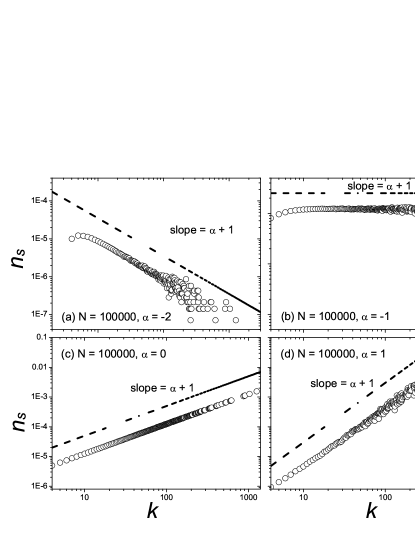
Figure 1: Log-log plot of the distribution of number of DSPs $n_{s}$ against the degree of node $k$ in black dots for PNNN-PIA with $m=4$, $C=1$ and $R=5$ for network size $N=10^{5}$ and preferential delivering exponents $\alpha$. The dashed line with slope $\alpha+1$ in each subplot is drawn for comparison purpose.

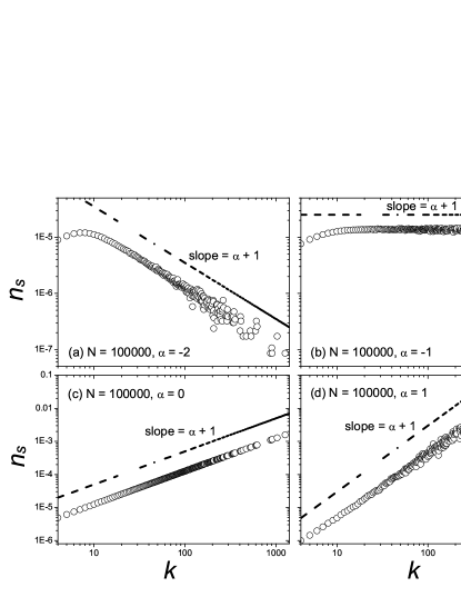
Figure 2: Log-log plot of the distribution of number of DSPs $n_{s}$ against the degree of node $k$ for PNNN+PIA. All parameters used are the same as those in Fig. 1.

III.2.1 Beyond The Simplifying Assumption

In reality, Eqs. (11) and (15) are not exact. Although it is much harder to modify the mean-field analysis in Sec. III.1 to take the PIA rule into account, we can still argued the behavior of the PNNN+PIA model qualitatively. First, we consider the effect of PIA rule on $n_{s}(k)$. Clearly, PIA rule makes $\Pi_{ji}$ in Eq. (7) historical path dependent. Thus, we can no longer apply the trick in Eq. (10) to give a simple expression for $n_{s}(k)$. Nevertheless, we may argue the behavior of $n_{s}(k)$ as follows. In the case of $\alpha<0$, Eq. (5) implies that packets are preferentially being forwarded to small degree nodes. However, the PIA rule forbids a packet to travel through the same edge more than twice. Therefore, compared with the situation without the PIA rule, a packet is less likely to be forwarded to a small degree node on average. On the other hand, the PIA rule has relatively little effect on high degree nodes. This is because of two reasons: first, packets are less likely to travel to these nodes; and second, packets located at these nodes generally have a large number of possible nodes to be forwarded to in the next time step. Thus, we expect that the same scaling behavior for $n_{s}(k)$ found in Eq. (11) is observed in the presence of PIA rule. Nonetheless, the domain of $k$ in which this scaling law holds is reduced as the value of the lower cutoff of the scaling law increases as a consequence of the PIA rule. Furthermore, below this lower cutoff point, the value of $n_{s}(k)$ is smaller that the case when the PIA rule is not adopted.

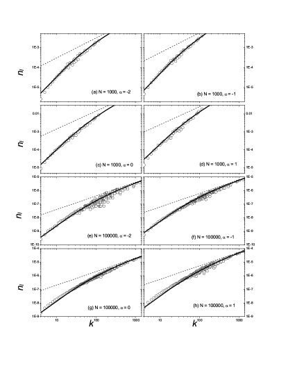
Figure 3: Log-log plot of the distribution of number of DLPs $n_{l}$ against degree of nodes $k$ for PNNN-PIA. The solid curve in each subplot is the prediction according to Eq. (15) with $\mu$ and $\nu$ treated as free fitting parameters. And the dotted line in each subplot is the asymptote of the corresponding solid curve. All parameters used in the simulations are the same as those in Fig. 1.

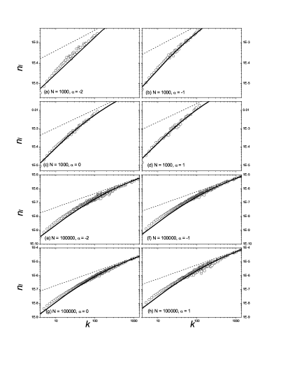
Figure 4: Log-log plot of the distribution of number of DLPs $n_{l}$ against degree of nodes $k$ for PNNN+PIA. The detailed procedure is adapted from the descriptions in Fig. 3.

Applying similar arguments in the previous paragraph to the case of $\alpha>0$, we conclude that it is more likely to forward a packet between two large degree nodes. Since the number of nodes with degree $k$ decreases as $k$ increases, the combination of Eq. (5) and the PIA rule will decrease (increase) the value of $n_{s}(k)$ in Eq. (11) for $k\lesssim k_{\max}$ ($k\ll k_{\max}$ and $k\gg k_{\min}$). Therefore, the domain in which the scaling behavior of Eq. (11) holds only for $k\ll k_{\max}$ and $k\gg k_{\min}$. To summarize, we have argued the validity of Eq. (11) in the large $N$ limit for the PNNN+PIA model over a reduced domain of $k$. In addition, the value of $\langle n_{s}(k_{i})\rangle_{i\in{\mathbb{V}}}$ decreases in the presence of PIA rule.

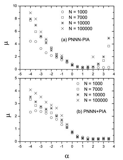
Figure 5: Plots of $\mu$ against $\alpha$ for (a) PNNN-PIA and (b) PNNN+PIA for various values of $N$.

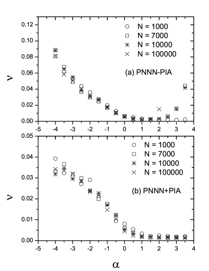
Figure 6: Plots of $\nu$ against $\alpha$ for (a) PNNN-PIA and (b) PNNN+PIA for various values of $N$.

How about the effect of PIA rule on $n_{l}(k)$? The PIA rule surely reduces both $\mu$ and $\nu$ by forbidding excessive routing through the same edge. Besides, the value of $\langle n_{s}(k_{i})\rangle_{i\in{\mathbb{V}}}$ is also reduced. But interestingly, unlike Eq. (7), the presence of PIA rule in no way affects the functional form of Eq. (15) as the derivation of Eq. (12) is also valid in this case. This is because the PIA rule cannot prevent a DLP from reaching its destination unless the distance between the destination and the initial generation point of the packet is less than two. (This is because at the first instance when a DSP is forwarded to a node $i$ with distance two from the packet destination. The DSP will turn into a DLP in the next time step. More importantly, this message packet must never pass through any shortest path connecting node $i$ and the packet destination. Hence, the PIA rule does not prevent this packet from moving along this shortest path.) And the probability for such case is negligible in the large $N$ limit. Note that $n_{l}(k)$ is more seriously affected by $\langle n_{s}(k_{i})\rangle_{i\in{\mathbb{V}}}$ than by $\mu$ or $\nu$. So, we expect that $n_{l}(k)$ decreases with the introduction of PIA rule. But its percentage decrease is not as large as that of $n_{s}(k_{\max})$.

We now move on to study the effect of PIA rule on the values of $\alpha_{c}$ and $R_{c}$. Recall that without PIA rule, $\alpha_{c}=-1$. Let us consider the case of $\alpha>-1$ first. In this case, both $n_{s}(k)$ and $n_{l}(k)$ are increasing functions of $k$ for $\alpha>-1$ with or without PIA rule. So, upon a gradual increase in the packet injection rate, the first node to congest must be the one with a large degree. From the arguments in this Subsection, we know that for $k\approx k_{\max}$, $n(k)\equiv n_{s}(k)+n_{l}(k)$ decreases with the introduction of PIA rule. Hence, the critical packet injection rate $R_{c}$ increases with the introduction of PIA rule. Certainly, the percentage increase in $R_{c}$ depends on the values of $N$, $m$ and $\alpha$ used; and the above arguments in no way imply that the percentage change is huge. Indeed, it is quite possible that the increase in $R_{c}$ is negligible in some cases.

In contrast, when $\alpha<-1$, Eq. (16) together with the arguments in this Subsection tell us that $n(k_{\min})\approx n_{s}(k_{\min})$ decreases more rapidly than $n(k_{\max})\approx n_{l}(k_{\max})\sim\left\langle n_{s}(k_{i})\right\rangle_{i\in{\mathbb{V}}}k_{\max}$ with the introduction of PIA rule. Consequently, $R_{c}$ increases in the presence of PIA rule. More importantly, for a finite $N$, one may find an $\alpha$ slightly less than $-1$ such that $n(k_{\min})<n(k_{\max})$. In other words, a large degree instead of a small degree node gets congested at $R_{c}$ for this value of $\alpha$. Therefore, we conclude that $\alpha_{c}$ decreases and $R_{c}$ increases in the presence of PIA rule. Note that once again the decrease in $\alpha_{c}$ may be insignificant in some cases.

Finally, we expect that the general trend of $R_{c}$ for PNNN-PIA described in Sec. III.2.1 also applies to PNNN+PIA. Obviously, our predictions are different from the numerical results of Yin et al. reported in Ref. Yin et al. (2006), which claimed that $R_{c}$ was a decreasing function of $\alpha$ for PNNN+PIA. In Sec. IV, we show that this is partly due to the fact that the network size $N$ used in their simulation is not large enough so that finite-size effect seriously affects their conclusions.

IV Comparison with our numerical simulations

We want to check the validity of our mean-field analysis reported in the previous Section as well as to to understand the origin of the discrepancy between our present work and the numerical results obtained by Yin et al. in Ref. Yin et al. (2006). And we do so by performing numerical simulations using larger values of $N$. Moreover, unlike Ref. Yin et al. (2006), we allow $R$ to take on non-integer values.

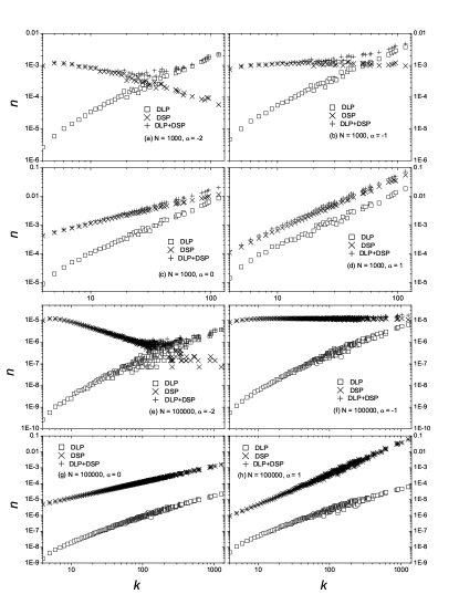
Figure 7: The average number of packets $n$ against degree of nodes $k$ for PNNN-PIA at $R=R_{c}$. All parameters used in the simulations are the same as those in Fig. 1.

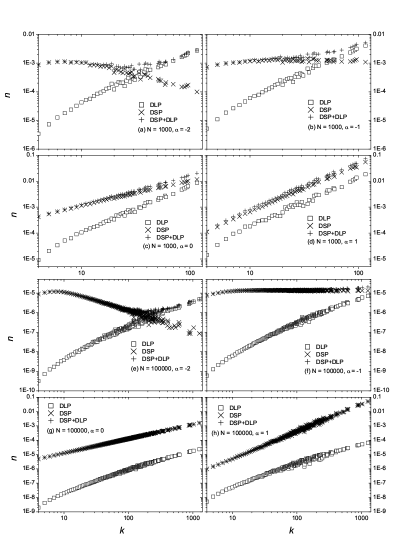
Figure 8: The average number of packets $n$ against degree of nodes $k$ for PNNN+PIA at $R=R_{c}$. All parameters used in the simulations are the same as those in Fig. 1.

Perhaps one of the reasons why Yin et al. reported numerical simulations of PNNN+PIA up to $N=5000$ only Yin et al. (2006) is that a lot of memory is needed to store the message packets present in the network as well as their historical paths. In fact, this straight-forward numerical simulation method is not practical for $N\gtrsim 10000$. Here we introduce a much less memory intensive way to numerically find $R_{c}$. Observe that the connectedness of BA network and the message forwarding rules of PNNN$\pm$PIA make the message packets in PNNN$\pm$PIA ergodic. Also, recall from Sec. II that message packets behave like independent particles as long as there are no more than $C$ packets staying in a node at any time. Although occasionally more than $C$ message packets may be present in a node in the free-flow phase, by ergodicity we expect that the statistical properties of PNNN$\pm$PIA below the critical packet injection rate $R_{c}$ can still be simulated by regarding each message packet as independent particle throughout. Therefore, the statistical behavior of PNNN$\pm$PIA for $R<R_{c}$ can be found as follows: We first numerically simulate the ensemble-averaged time evolution of a particular free-flow phase situation in which there is exactly one message packet in the network at all times. By ergodicity, the ensemble-averaged number of packet present in a node obtained in the above simulation equals the (time-averaged) number of packet in that node when the packet injection rate $R$ is $1/\langle\tau\rangle$, where $\langle\tau\rangle$ denotes the mean packet lifetime. (This choice of $R$ does not contradict with the prediction of Eqs. (30b) and (30c) that $R_{c}\rightarrow 0$ in the limit of large $N$ whenever $\alpha>\alpha_{c}$. This is because the mean packet lifetime $\langle\tau\rangle$ scales like $N^{\beta}$ with $\beta\geq 2$.) Below the critical packet injection rate $R_{c}$, the distributions $n_{s}(k)$, $n_{l}(k)$ and $n(k)$ are directly proportional to the packet injection rate $R$. Consequently, $R_{c}$ is equal to $C/\langle\tau\rangle\max_{k}n(k)$ where $\max_{k}n(k)$ is the maximum value of $n(k)$ over all $k$ for the case of $R=1/\langle\tau\rangle$. Clearly, this method can compute $R_{c}$ accurately and efficiently. As only one message packet is used at any time in the simulation, this method requires much less memory than the straight-forward numerical simulation approach. We further verify the validity of this ensemble-averaged simulation method by successfully reproducing the numerical simulation results reported by Yin et al. in Ref. Yin et al. (2006) (modulo the fact that they restricted $R$ to integers). (Actually, the value of $m$ used for their PNNN-PIA simulation is 4 instead of 5 Yin and Wang (2009).) Therefore, we adopt this new method in our subsequent numerical studies.

While the simulations of Yin et al. in Ref. Yin et al. (2006) was performed in for $\alpha\in[-4,2]$, ours is done in a slightly large parameter range of $[-4,4]$. Actually, we find that the bias in forwarding a DSP according to Eq. (5) for $|\alpha|$ close to $4$ is already so high that the data obtained from our simulations are no longer very reliable. And reliable results for $|\alpha|\gtrsim 4$ has to be obtained by much longer simulation time with the aid of a higher precision pseudo random number generator.

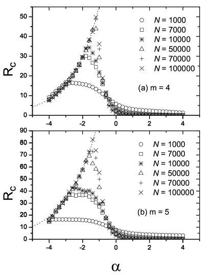
Figure 9: The $R_{c}$ against $\alpha$ curve for PNNN-PIA with $C=1$ and (a) $m=4$, and (b) $m=5$. The dashed curve in each subplot is our mean field analytical prediction based on Eq. (30a). More precisely, the dashed curve is the best fit curve obtained from Eq. (30a) by treating $\Xi$ as a free parameter independent of $\alpha$.

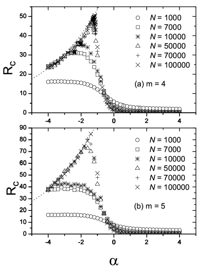
Figure 10: The $R_{c}$ against $\alpha$ curve for PNNN+PIA. Parameters used are the same as those in Fig. 9.

Let us begin by checking the validity of our assumptions made in Sec. III. Figs. 1 and 2 show typical $n_{s}(k)$ curves obtained from our numerical simulations of PNNN-PIA and PNNN+PIA, respectively. They show that $n_{s}(k)$ indeed follows a power law with exponent $\alpha+1$ over most of the parameter range for PNNN$\pm$PIA for sufficiently large $N$. Furthermore, the domain of validity of the power law is reduced with the introduction of PIA rule. More importantly, in the case of PNNN+PIA, the ways how $n_{s}(k)$ deviates from the power law for small and large $k$ are consistent with our predictions in Sec. III.2. That is to say, $n_{s}(k)$ is less (greater) than the value obtained by Eq. (11) for $k\approx k_{\min}$ ($k\approx k_{\max}$). In this respect, our assumption of ignoring degree-degree correlation between neighboring nodes in obtaining $n_{s}(k)$ is not bad.

Next, we examine the validity of Eq. (15) for PNNN$\pm$PIA. Figs. 3 and 4 plot $n_{l}$ as a function of $k$ obtained from our simulation of PNNN-PIA and PNNN+PIA, respectively. Our simulation results for $n_{l}(k)$ agree quite well with the solid curves, namely, our mean field prediction given by Eq. (15). The dotted lines in Figs. 3 and 4 show the asymptotic behavior of the solid curve in the limit of large $k$. By comparing our simulated data points with the dotted lines, we find that for $N$ as small as $1000$, $n_{l}(k)$ does not reach the linear scaling regime at all. And for $N=100000$, $n_{l}(k)$ attains linear scaling for $k\gtrsim 200$. In fact, we discover from our simulation that $n_{l}(k)$ scales like a linear function of $k$ around $k\lesssim k_{\max}$ only when $N\gtrsim 10000$.

As shown in Figs. 5 and 6, $\mu$ and $\nu$ are independent of $N$ for PNNN$\pm$PIA provided that $N\gtrsim 7000$ and $|\alpha|\lesssim 3$. We believe that the discrepancy for $\mu$ when $N=1000$ in Fig. 5 is the result of finite size effect. And as we have already discussed earlier in this Section, we think that the discrepancies for $\mu$ and $\nu$ for $|\alpha|\gtrsim 3$ are due to the limitations of our simulation time and pseudo random number generator used. In any case, Figs. 5 and 6 verify that $\mu$ and $\nu$ are not sensitively dependent on $\alpha$. In fact, $\mu$ and $\nu$ are of order of $1$ and $0.01$ respectively over most of the range of $\alpha$ we have studied. And in line with our expectation, $\mu$ and $\nu$ decrease with the introduction of PIA rule.

Figs. 7 and 8 depict the general trend of $n_{s}(k)$, $n_{l}(k)$ and $n(k)=n_{s}(k)+n_{l}(k)$ near $R=R_{c}$ for PNNN-PIA and PNNN+PIA, respectively. They show that for a sufficiently small $\alpha$, the degree of the congested node at $R=R_{c}$ is generally close but not equal to $k_{\min}$. This is not surprising because there are numerous nodes with degree close to $m$. Local conditions such as the degrees of the neighbors of these small degree nodes can vary a lot. Combined with the break down of the scaling relation in Eq. (11), jamming may occur at a node whose degree is slightly greater than $k_{\min}$ when $R=R_{c}$. In contrast, Figs. 7 and 8 show that for a sufficiently large $\alpha$, jamming almost always occurs in the highest degree node in the network. This is because for a generic BA network with a large but fixed $N$, there is a considerable difference between the degree of the most connected and second most connected nodes. Thus, $n_{l}$ for the most connected node is almost surely greater than that for the slightly less connected ones. Most importantly, our simulations find that the transition between these two types of congested nodes at $R=R_{c}$ occurs at a rather well-defined critical $\alpha_{c}$ for $N\gtrsim 1000$. And the value of $\alpha_{c}$ depends on the value of $N$ as well as on whether the PIA rule is adopted or not.

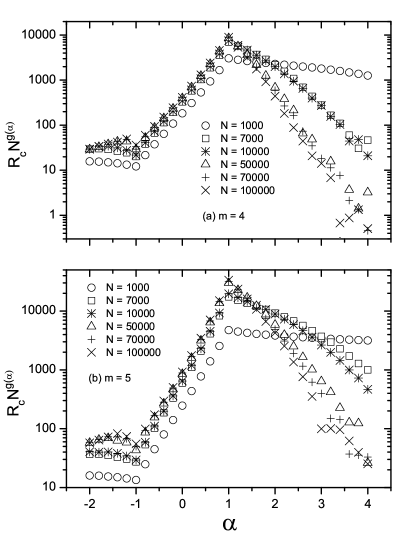
Figure 11: The $R_{c}N^{g(\alpha)}$ against $\alpha$ curve for PNNN-PIA. Parameters used are the same as those in Fig. 9.

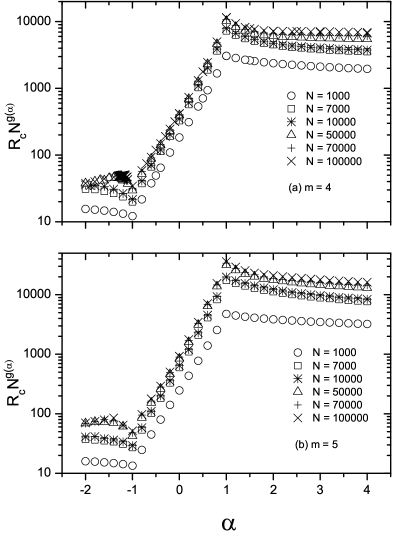
Figure 12: The $R_{c}N^{g(\alpha)}$ against $\alpha$ curve for PNNN+PIA. Parameters used are the same as those in Fig. 9.

After finish justifying the validity of the approximations made in our mean field analysis, we now move on to compare our mean field calculations and numerical simulation results with the numerical findings of Yin et al. reported in Ref. Yin et al. (2006). As the $R_{c}$ against $\alpha$ curves in Figs. 9 and 10 shown, the general trend of $R_{c}$ we find in our numerical simulations agrees quite well with the predictions of our mean field theory for both PNNN-PIA and PNNN+PIA. In particular, we discover that for fixed $N$ and $m$, $R_{c}$ is an increasing (decreasing) function of $\alpha$ for $\alpha<\alpha_{c}$ ($\alpha>\alpha_{c})$. Besides, $\alpha_{c}$ decreases and $R_{c}$ increases with the introduction of PIA rule although the change is not significant for large $N$ and small $m$. Recall from Eq. (30a) and the discussions in Sec. III.2.1 and III.2 that in the large $N$ limit, $\Xi$ should be roughly a constant over the parameter range of interest and $R_{c}$ should roughly scales like $1/(1-\alpha)$ whenever $\alpha<\alpha_{c}$. This is exactly what we find in Figs. 9 and 10. More generally, Eqs. (30a)–(30c) imply that $R_{c}N^{g(\alpha)}$ should be $N$ independent, where

$$g(\alpha)=\left\{\begin{array}[]{ll}0&\enspace\mbox{for}\enspace\alpha<-1,\\ (\alpha+1)/2&\enspace\mbox{for}\enspace-1<\alpha<1,\\ 1&\enspace\mbox{for}\enspace\alpha>1.\end{array}\right.$$ (31)

As shown in Figs. 11 and 12, $R_{c}N^{g(\alpha)}$ is indeed $N$ independent for $\alpha<1$ ($\alpha>1$) provided that $N\gtrsim 10000$ ($N\gtrsim 500000$). Again, the discrepancy for $\alpha>3$ is probably caused by insufficient sampling and the finite precision of our pseudo random number generator.

As for the critical preferential delivering exponent $\alpha_{c}$, we find that it decreases as $m$ increases for a fixed $N$. This can be explained as follows: Recall that the number of 4-cycles in a BA network scales like $\left[m\log(N)/2\right]^{4}/4$ Bianconi (2004). So, by increasing $m$ while fixing $N$, the proportion of 4-cycles in the network increases. In other words, the assumption of neglecting the effect of 4-cycles in our mean-field analysis reported Sec. III becomes less valid. By going through the analysis in Sec. III once more, it is not difficult to see that although the scaling relations in Eqs. (11) and (16) are robust against the presence of 4-cycles, the $(k-1)$ factor in Eq. (15) should be replaced by $(k-\zeta)$ for some $\zeta>1$. This change decreases the value of $n_{l}(k)$ for a fixed $N$, therefore making the small degree node harder to jam. This is the reason why the presence of large number of 4-cycles reduces the value of $\alpha_{c}$.

In the case of $m=4$, Figs. 9(a) and 10(a) show that $\lim_{N\rightarrow\infty}\alpha_{c}$ is very close to $-1$ for PNNN$\pm$PIA. Combined with the validity of Eqs. (30a) and (30b) as depicted in Figs. 11(a) and 12, we conclude that $R_{c}$ approaches to its maximum value at $\alpha_{c}=-1$ in the large $N$ limit. In contrast, for simulation up to $N=100000$, $\alpha_{c}$ does not seem to converge to $-1$ in the case of $m=5$. As we have discussed in the last paragraph, we believe that this is due to the existence of large amount of 4-cycles. Since for $m=5$, the number of 4-cycles is less than about $N/10$ provided that $N\gtrsim 10^{7}$, we believe that $\alpha_{c}$ should converge to $-1$ by using networks at least about 100 times larger than our currently used ones. Unfortunately, such simulation is beyond the current computing capacity of our group.

Now, let us compare our findings with that of Yin et al.’s in Ref. Yin et al. (2006). Fig. 10 show that the simulations performed on a $N=1000$ network does not reveal the thermodynamic behavior of the system due to serious finite size corrections. Actually, if they had extended their numerical simulations to $\alpha$ as small as about $-8$ (which unfortunately requires much longer computational time and the use of a high precision pseudo random number generator), they should have revealed the maximum point on the $\alpha-R_{c}$ curve, thereby discovering the critical $\alpha_{c}$.

V Discussions

To summarize, we have pointed out that the PNNN+PIA model is not a good model of network traffic due to the hidden communication cost involved. In addition, we have carefully performed a mean-field analysis of the message packet dynamics for a network traffic model with PNNN routing strategy on BA network with or without PIA by Yin et al. in Ref. Yin et al. (2006). The main feature of our analysis is that we divide the message packets into two groups, namely, the DSPs and DLPs. To check the validity of our mean-field results, we introduce a new method to simulate the critical packet injection rate $R_{c}$ that requires much less memory. This enable us to carry out an extensive numerical simulation to study the so-called $\alpha-R_{c}$ curve for larger network size $N$ with the message packet injection rate $R$ taking on real rather than integer values.

For a fixed finite network size $N$, we discover that the $\alpha-R_{c}$ curve is in fact increasing (decreasing) for $\alpha<\alpha_{c}$ ($\alpha>\alpha_{c}$). And we are able to explain this behavior by means of our mean-field analysis. In fact, both our mean-field calculations and our numerical simulations show that the critical message generation rate $R_{c}$ attains its maximum value at $\alpha_{c}=-1$ for models both with and without PIA rule in the limit of large $N$. In this respect, the role of PIA rule has little effect on the $\alpha-R_{c}$ curve even though the value of $R_{c}$ is increased by introducing the PIA rule. At the same time, Eq. (30a) tells us that $R_{c}$ is independent of $N$ in the limits of $N\rightarrow\infty$ and $\alpha\rightarrow-1^{-}$. This means that the PNNN mechanism is not efficient in handling large scale BA network traffic. In fact, this result agrees with those of Sreenivasan et al. Sreenivasan et al. (2007) who showed that $R_{c}\leq O(\sqrt{N})$ for a BA network with any routing strategy.

One may apply our analysis to consider the extension of PNNN$\pm$PIA to the case in which more extended local information of the network such as the third nearest neighbors is used to forward a packet. It is not too difficult to argue that $n_{s}(k)\sim k^{\alpha+1}$ and $n_{l}(k)\sim k$ in the large $N$ limit for this kind of models. Thus, it appears that straight-forward generalizations of the PNNN packet forwarding rule are also not efficient to handle large scale BA network traffic in the sense that the resultant maximum possible value of $R_{c}$ is independent of $N$. One has to find other type of strategies in order to approach the upper bound of $O(\sqrt{N})$ for $R_{c}$.

In addition to the functional dependence of $R_{c}$ on $\alpha$, it is instructive to study the nature of the phase transition between the free-flow and jamming phases in PNNN$\pm$PIA. Nonetheless, our mean field analysis and the trick used in our extensive numerical simulations are for free-flow phase only. Further work has to be done to investigate this problem.