Hyperaccreting Neutron-Star Disks, Magnetized Disks and Gamma-Ray Bursts

Hyperaccreting Neutron-Star Disks

Magnetized Disks

and Gamma-Ray Bursts

Dong Zhang

Professor Zi-Gao Dai

Nanjing, China

For the memory of my Grandfather

Abstract

Gamma-ray bursts (GRBs) have been an enigma since their discoveries forty years ago. What are the nature of progenitors and the processes leading to formation of the central engine capable of producing these huge explosions? My thesis focus on the hyperaccreting neutron-star disks cooled via neutrino emissions as the potential central engine of GRBs. I also discuss the effects of large-scale magnetic fields on advection and convection-dominated accretion flows using a self-similar treatment. This thesis is organized as follows:

In Chapter 1, we first present a brief review on the theoretical models of GRB for forty years. Although GRBs were first considered from supernovae at cosmological distances, Galactic models become more popular in 1980s, particularly after the detections of cyclotron absorption and emission lines by the Konus and Ginga detectors, which showed that neutron stars with magnetic fields $\sim 10^{12}$ G are the most possible sources of GRBs. Galactic GRBs were purposed to be produced from stellar flares or giant stellar flares from main sequence or compact stars, from starquakes of neutron stars, from accretion processes and thermonuclear burning onto neutron stars, from collapses of white dwarfs and so on. It was not until the mid-1990s that the observation results by BATSE strongly suggested that GRBs originate at cosmological distance. The main Cosmological GRB models include the mergers of neutron star binaries and black hole-neutron star binaries, the “collapsar" model (i.e., the collapses of massive star), the magnetar model, and the quark stars and strange stars model. We distinguish GRB progenitors and its direct central engines. Furthermore, we discuss two GRB progenitor scenarios in detail: the collapsar scenario for long-duration bursts, and compact start merger scenario for short-hard bursts.Observation evidence supports the hypothesis that long-duration GRBs are supernova-like phenomena occurring in star formation region related to the death of massive stars. Their energy is concentrated in highly relativistic jet. We investigate various collapsar formation scenarios, the requirements of collapsar angular momentum and metallicity for generating GRBs, and the relativistic formation, propagation and breakout in collapsars. Mergers of compact objects due to gravitational radiation as the sources of short-hard GRBs have been widely studied for years. We present the neutron star-neutron star, black hole-neutron star and white dwarf-white dwarf binaries as the most possible progenitors of short bursts. We also introduce the numerical simulations results of merges of the three types of binaries. In addition to the above progenitor scenarios, we also mention the “supranova" and magnetar scenario.

Most GRB progenitor scenarios lead to a formation of a stellar-mass black hole and a hyperaccretion disk around it. This accreting black hole system is commonly considered as the direct central engine of GRBs. In Chapter 2 we discuss the physical properties of accretion flows around black holes. Accretion flows may be identified in three cases: cooling-dominated flows, advection-dominated or convection-dominated flows, and advection-cooling-balance accretion flows. On the other hand, accretion flows can be classified by their cooling mechanisms: no radiation, by photon radiation, or by neutrino emission. We first investigate the structure of the normal accretion disks, which could be cooled by photon radiation effectively, and then we discuss the similar structure of advection and convection-dominated flows. Next we describe the main thermodynamical and microphysical processes in neutrino-cooled disks, and show the properties of such neutrino-cooled flows around black holes. Moreover, we discuss the two mechanisms for producing relativistic jets from the accreting black holes: neutrino annihilation and MHD processes, especially the Blandford-Znajek process.

Chapter 3-5 are my works on hyperaccretion neutron star-disks and magnetized accretion flows. As mentioned in Chapter 2, it is usually proposed that hyperaccretion disks surrounding stellar-mass black holes, with an accretion rate of a fraction of 1 $M_{\odot}$ s^-1 are central engines of GRBs. In some models, however, newborn compact objects are introduced as neutron stars rather than black holes. Thus, hyperaccretion disks around neutron stars may exist in some GRBs. Such disks may also occur in Type II supernovae. In Chapter 3 we study the structure of a hyperaccretion disk around a neutron star. Because of the effect of a stellar surface, the disk around a neutron star must be different from that of a black hole. Clearly, far from the neutron star, the disk may have a flow similar to the black hole disk, if their accretion rate and central object mass are the same. Near the compact object, the heat energy in the black-hole disk may be advected inward to the event horizon, but the heat energy in the neutron star disk must be eventually released via neutrino emission because the stellar surface prevents any heat energy from being advected inward. Accordingly, an energy balance between heating and cooling would be built in an inner region of the neutron star disk, which could lead to a self-similar structure of this region. We therefore consider a steady-state hyperaccretion disk around a neutron star, and as a reasonable approximation, divide the disk into two regions, which are called inner and outer disks. The outer disk is similar to that of a black hole and the inner disk has a self-similar structure. In order to study physical properties of the entire disk clearly, we first adopt a simple model, in which some microphysical processes in the disk are simplified, following Popham et al. and Narayan et al. Based on these simplifications, we analytically and numerically investigate the size of the inner disk, the efficiency of neutrino cooling, and the radial distributions of the disk density, temperature and pressure. We see that, compared with the black-hole disk, the neutron star disk can cool more efficiently and produce a much higher neutrino luminosity. Finally, we consider an elaborate model with more physical considerations about the thermodynamics and microphysics in the neutron star disk (as recently developed in studying the neutrino-cooled disk of a black hole), and compare this elaborate model with our simple model. We find that most of the results from these two models are basically consistent with each other.

In Chapter 4 we further study the structure of such a hyperaccretion neutron-star disk based on the two-region (i.e., inner & outer) disk scenario following Chapter 3, and calculate the neutrino annihilation luminosity from the disk in various cases. We investigate the effects of the viscosity parameter $\alpha$, energy parameter $\varepsilon$ (measuring the neutrino cooling efficiency of the inner disk) and outflow strength on the structure of the entire disk as well as the effect of emission from the neutron star surface boundary emission on the total neutrino annihilation rate. The inner disk satisfies the entropy-conservation self-similar structure for the viscosity parameter $\varepsilon\simeq 1$ and the advection-dominated structure for $\varepsilon<1$. An outflow from the disk decreases the density and pressure but increases the thickness of the disk. Moreover, compared with the black-hole disk, the neutrino annihilation luminosity above the neutron-star disk is higher, and the neutrino emission from the boundary layer could increase the neutrino annihilation luminosity by about one order of magnitude higher than the disk without boundary emission. The neutron-star disk with the advection-dominated inner disk could produce the highest neutrino luminosity while the disk with an outflow has the lowest. As a result, the neutrino annihilation above the neutron-star disk may provide sufficient energy to drive GRBs and thus observations on GRB-SN connection could constrain the models between hyperaccreting disks around black holes and neutron stars with outflows.

In Chapter 5, we study the effects of a global magnetic field on viscously-rotating and vertically-integrated accretion disks around compact objects using a self-similar treatment. We extend Akizuki & Fukue’s work (2006) by discussing a general magnetic field with three components ($r,\varphi,z$) in advection-dominated accretion flows (ADAFs). We also investigate the effects of a global magnetic field on flows with convection. For these purposes, we first adopt a simple form of the kinematic viscosity $\nu=\alpha c_{s}^{2}/\Omega_{K}$ to study magnetized ADAFs: a vertical and strong magnetic field, for instance, not only prevents the disk from being accreted but also decreases the isothermal sound speed. Then we consider a more realistic model of the kinematic viscosity $\nu=\alpha c_{s}H$, which makes the infall velocity increase but the sound speed and toroidal velocity decrease. We next use two methods to study magnetized flows with convection, i.e., we take the convective coefficient $\alpha_{c}$ as a free parameter to discuss the effects of convection for simplicity. We establish the $\alpha_{c}-\alpha$ relation for magnetized flows using the mixing-length theory and compare this relation with the non-magnetized case. If $\alpha_{c}$ is set as a free parameter, then $|v_{r}|$ and $c_{s}$ increase for a large toroidal magnetic field, while $|v_{r}|$ decreases but $|v_{\varphi}|$ increases (or decreases) for a strong and dominated radial (or vertical) magnetic field with increasing $\alpha_{c}$. In addition, the magnetic field makes the $\alpha_{c}-\alpha$ relation be distinct from that of non-magnetized flows, and allows the $\rho\propto r^{-1}$ or $\rho\propto r^{-2}$ structure for magnetized non-accreting convection-dominated accretion flows with $\alpha+g\alpha_{c}<0$ (where $g$ is the parameter to determine the condition of convective angular momentum transport).

Finally, we give an outlook in Chapter 6.

Chapter 1 GRB Progenitors

1.1 Detectors and Observations

Theoretical astrophysics is always based on the observation events and data. In §1.1 we list the detectors of Gamma-ray bursts (GRBs) and their main contributions. The theories of GRBs are based on these observations.

$\blacksquare$Vela Satellites

The total number of Vela Satellites is 12, six of the Vela Hotel design, and six of the Advanced Vela design, launched from October 1963 to April 1970. These military satellites were equipped with X-ray detectors, $\gamma$-ray detectors and neutron detectors, and the advanced ones also with the silicon photodiode sensors. The first flash of gamma radiation sinal was detected by Vela 3 and Vela 4 on July 2, 1967. Further investigations were carried out by the Los Alamos Scientific Laboratory, lead by Ray Klebesadel. They traced sixteen gamma-ray bursts between 1969 July and 1972 July, using satellites Vela 5 and Vela 6, and reported their work in 1973 (Klebesadel et al. 1973).

$\blacksquare$ First IPN (Inter-Planetary Network)

The investigation of the new phenomenon gamma-ray bursts become a fast growing research area after 1973. Beginning in the mid seventies, second generation gamma-ray sensors started to operate. By the end of 1978, the first Inter-Planetary Network had been completed. In addition to the Vela Satellites, gamma-ray burst observations were conducted from Russian Prognoz 6,7, the German Helio-2, NASA’s Pioneer Venus Orbiters, Venera 11 and Venera 12 spacecrafts. A group from Leningard using the KONUS experiment aboard Venera 11 and Venera 12 did significant work for gamma-ray burst survey. The important results of the first IPN projects include:

(1) First survey of GRB angular and intensity distribution by KONUS experiments (Matzet et al. 1981).

(2) Discovery of first SGR (SGR 0526-66, Mazet et al. 1979, Cline et al. 1980).

(3) Cyclotron and annihilation lines observations for many bursts (Mazets et al. 1981). The absorption and emission lines observation raised lots of debates until the discovery of cyclotron absorption lines by Ginga in 1988.

$\blacksquare$ Ginga

Ginga was an X-ray astronomy satellite launched on February 1987. Cyclotron features in the spectra of three GRBs (Murakami et al. 1988, Fenimore et al. 1988, Yoshida et al. 1991) were reported and interpreted as photon scattering process near the neutron star surface with strong magnetic fields $\sim 1.7\times 10^{12}$ G. Neutron-Star model become popular in those years. Moreover, Ginga data also provided the early evidence of the existence of X-ray Flashes (XRFs, Strohmayer et al. 1998), which were discussed in detailed in the BeppoSAX era.

$\blacksquare$ Compton Gamma-Ray Observatory (CGRO)

The Compton Gamma Ray Observatory (CGRO) is part of NASA’s Great Observatories. CGRO carried a complement of four instruments which covered observational band from 20keV to 30GeV, and the Burst and Transient Source Experiment (BATSE) is one of them. BATSE become the most ambitious experiment to study GRBS before BeppoSAX. It had detected a total of 2704 GRBs from April 1991 to June 2000, which provided a large sample for GRBs statistical work. Several significant results concerning the characteristics of GRBs were made based on the crucial data from BATSE. The cosmological GRB orgin was first established, although the debate between galactic and cosmological origin still continued until BeppoSAX. Moreover, the bimodality of GRB durations was established by analyzing the distribution of $T_{90}$ for hundreds of BATSE-observed-GRBs.

(1) The several BATSE catalogs had confirmed the apparent isotropy of the GRB spatial distribution (Meegan et al. 1992). Then the cosmological origin of GRBs began to be accepted by most astronomers. The energy of GRBs is about $10^{52}$ergs.

(2) BATSE data showed that GRBs were separated into two classes: short duration bursts ($T_{90}<$2s) with predominantly hard spectrum and long duration bursts ($T_{90>}$2s) with softer spectrum (Kouveliotou et al. 1993). Next two different classes of progenitors were suggested for this distinction: mergers of neutron star binaries (or neutron star and black hole systems) for short bursts, and collapse of massive stars for long bursts. however, some others believe there are three kinds of GRBs also based on the BASTE data, which should reflect three different types of progenitors (Mukherjee et al. 1998).

$\blacksquare$ BeppoSAX

BeppoSAX was an Italian-Dutch satellite for X-ray and gamma-ray astronomy. It was launched in 1996 and ended its life in 2003. This instrument had led to the discoveries of many new features of gamma-ray bursts and greatly accelerated people’s understanding about GRBs:

(1) The discovery of the X-ray afterglow of GRBs, which opened the afterglow era with multi-wavelength observations and confirmed the cosmological origin of GRBs. BeppoSAX first detected GRB 970228 with its X-ray afterglow (Costa et al. 1997), and later optical afterglow was also detected by the ground-based telescopes. Next, Keck II detected the spectrum of optical afterglow of GRB 970508, registered by BeppoSAX, and determined a redshift of $z=0.835$, which confirmed a cosmological distance (Metzger et al. 1997).

(2) The connection between GRBs and Type Ib/c supernove (SNe Ib/c). In 1998 BeppoSAX with the ground-based optical telescopes provided the first clue of a possible connection between GRB 980425 and a new supernova SN 1998 bw (Galama et al. 1998).

(3) The confirmation of a new sub-class of GRBs–X Ray Flashes (XRFs), which emit the bulk of their energy around a few Kev, at energies significantly lower than the normal GRBs (Heise et al. 2001). Furthermore, BeppoSAX first reported the detection of the X-ray-rich GRBs (Frontera et al. 2000).

(4) The discovery of GRBs with bright X-ray afterglows but no detectable optical afterglows, i.e. the ’dark bursts’. The next instrument HETE-2 made a more detailed detection on ’dark bursts’.

(5) The discovery of the possible correlation between the isotropic equivalent energy radiated by GRBs and the peak energy, such as Amati relation (Amati et al. 2002) and Ghirlanda relation (Ghirlanda et al. 2004), provided the new possible standard candles to measure the Universe with parameters.

$\blacksquare$ HETE-2

The first High Energy Transient Explorer (HETE-2) failed during the launch in 1996 and lost the opportunity to explore the significant characteristics of GRBs before BeppoSAX. However, the second HETE, HETE-2, with multiwavelength instruments, had got many achievements. It first confirmed a event of GRB-SN connection (GRB 030329 & SN 2003dh, Stanek et al. 2003). It first discovered a short-hard GRB with an optical counterpart (GRB 050709) and studied the afterglow properties of short bursts together with Swift. Moreover, it studied the phenomena XRFs more detailed than BeppoSAX.

$\blacksquare$ Swift

Swift is a multi-wavelength space-based observatory dedicated to the study of GRBs. It contains three instruments work together to observe GRBs and their afterglows in the gamma-ray, X-ray, ultraviolet and optical wavebands: the BAT (Burst Alert Telescope) detects GRBs events in the energy range between 15 keV to 150 keV, and computes its coordinates in the sky; the XRT (X-ray telescope) takes imagines and performs spectral analysis of the GRB X-ray afterglows in the energy range from 0.2 to 10 keV; and the UVOT (Ultriviolert/Optical Telescope) is used to detect an optical afterglow after Swift has slewed toward a GRB. This satellite was launched in November 2004 and is still in operation. The major breakthroughs from Swifts up to this date include:

(1) established a completely new view of the early X-ray afterglow with several well-defined phases: after the prompt emission there is a rapid decline phase, which is followed by a shallow decay phase combined with X-ray flares, and then is the normal decay phase. Moreover, Swift has detected the existence of the achromatic breaks, causing some issues of the jet break interpretation of the break phase of X-ray afterglows.

(2) detected GRBs with high-redshift, e.g., GRB 050904 with $z$=6.29 (Price et al. 2006), GRB 080913 with $z$=6.7 (Schady et al. 2008). These detections provide a unique way of probing the Universe when the first stars were formed. Combined with the observation by Hubble and Spitzer, Swift

(3) first observed the afterglows of short hard GRBs (GRB 050509b, Hjorth et al. 2005).

(4) the discovery of GRB 060614 called for a rethink of the GRB classification. GRB 060614 is a burst with $T_{90}=104$s other properties like short bursts. The classification of GRBs should based on their afterglows, host galaxies, not only their durations of prompt emission (e.g., Zhang 2006).

Figure 1.1: Some former and current GRB detectors. First row (left to right): Vela 5B (1969-1979), Ginga (1987-1991), CGRO/BATSE (1991-2000); second row: Konus-Wind (1994- ), BeppoSAX (1996-2003), HETE-2 (2000- ); third row: INTEGRAL (2002- ), Swift (2004- ), Fermi (2008- ).

$\blacksquare$ Current Missions

In addition to the Swift satellite, there are also many present missions to study GRBs. The present long-baseline GRB IPN, i.e., the third IPN, includes Ulysses in 1992, Konus-wind in 1994, Rossi XTE in 1995, HETE-2 in 2000, Mars Odgssey in 2001, RHESSI in 2002, INTEGRAL in 2002, Swift in 2004, MESSENGER in 2004, Suzaku in 2005, AGILE in 2007 and Fermi in 2008. On the other hand, BATSE-CGRO (1991-2000), SROSS-C2 (1994-2001?), SZ-2 (2001), NAER (1996-2001), BeppoSAX (1996-2003) and SZ-2 (2001) have ceased operations today. Here I list some significant missions in this subsection.

• Konus-Wind

  The joint Russian-American Konus-Wind experiment is presently carried out onboard the NASA’s Wind spacecraft, which was launched in November 1994 and mainly to study the ’solar wind’. The Konus experiment on Wind satellite, provides omnidirectional and continuous coverage of the entire sky in the hard X- and gamma-ray domain. Konus also provides the only full-time near-Earth vertex in the present IPN project. Konus-Wind has detected thousands of GRBs since 1994 until now.

• INTEGRAL

  The European Space Agency’s International Gamma-Ray Astrophysics Laboratory (INTEGRAL), launched in 2002, is a successor to CGRO. It can similarly determine a coarse position by comparing gamma counts from one side to another. It also possesses a gamma-ray telescope with an ability to determine positions to under a degree. The science achievements of INTEGRAL has covered many areas in gamma-ray astronomy, the observations of GRBs made by INTEGRAL over the last years includes the discovery of the nearby low energy GRB 031203 (Gotz et al. 2003).

• RHESSI

  RHESSI was launched in 2002 to perform solar studies. However, its gamma instrument could detect bright gamma sources from other regions of the sky, and produce coarse positions through differential detectors. For instance, RHESSI observed 58 bursts in 2007 and 34 in the first 9 months in 2008.

• AGILE

  This X-ray and Gamma ray astronomical satellite, launched in April 2007 and equipped with scientific instruments capable of imaging distant celestial objects in the X-ray and Gamma ray regions of the electromagnetic spectrum, is adding data to the third IPN.

• Fermi

  The Fermi Gamma-ray Space Telescope is a space observatory being used to perform gamma-ray astronomy observations from low Earth orbit. Its main instrument is the Large Area Telescope (LAT), with which astronomers mostly intend to perform an all-sky survey studying of gamma radiation high-energy sources and dark matter. Another instrument, the Gamma-ray Burst Monitor (GBM), is being used to study GRBs.

1.2 A Review of GRB Models

Gamma-ray bursts have been an enigma since their discoveries forty years ago. What are the nature of progenitors and the processes leading to formation of the central engine capable of producing these huge explosion? The first GRB model was published (Colgate 1968) even before the discovery of these burst events by Vela in 1969. This model suggested that transient prompt gamma-rays and X-rays would be emitted as Doppler-shifted Planck radiation from the relativistically expanding outer layers of supernovae. Klebesadel et al. (1973) discussed the possibility that GRBs are associated with some particular supernovae which are not bright in the optical band (Thorne 1968) in the first observation paper of GRBs. However, it was not until 25 years later when BeppoSAX could detect the connection between GRB 980425 and SN 1998bw. Hawking (1974) showed that black holes would create and emit particles like photons and evaporate themselves. In this point of view, gamma-ray bursts could provide the direct evidence of the existence of black holes. However, today we know this physical opinion could not explain most GRBs, after we accumulated sufficient observation evidence of bursts.

Although GRBs were first considered at cosmological distances from supernovae, Galactic models became more popular at later time, particularly after the detections of cyclotron absorption and emission lines by Konus and Ginga (Mazets et al. 1981; Murakami et al. 1988). More than one hundred GRB Galactic models had been published before 1990s. The early observations (1st IPN, Ginga, etc.) led to considering neutron stars with strong magnetic fields as ideal candidates for GRBs sources. Moreover, the neutron star models were also reinforced by the discoveries of SGR.

However, on the other hand, Paczyński and a few other astronomers pointed out again the idea that gamma-ray bursts could be at cosmological distances like quasars, with redshifts around 1 to 2 (Paczyński 1986; Goodman 1986). The energy needed was comparable to the energy typically released by a supernovae. Their cosmological model was based on the evidences of GRBs isotropy spatial distribution and deviation of the intensity distribution from the -3/2 law, both of which were still controversial in 1980s, but crucially confirmed by BATSE-CGRO in 1990s. The observation results by BATSE in mid-1990s strongly suggested that the bursts originate at cosmological distance. Thanks to BeppoSAX and the discovery of afterglows with redshifts, the cosmological nature of GRBs has been well established since 1997.

BeppoSAX with the multi-wavelength observations on the afterglows raised researchers interests in explaining the lightcurve and spectrum using various radiation processes during and after bursts; and the models of GRB progenitors and central engines became less than before. Currently, the most widely-accepted model for the origin of most observed long GRBs is called the “collapsar" model (Woosley 1993), in which the core of an extremely massive, low-metallicity, rapidly-rotating star collapses into a compact object. On the other hand, short hard GRBs are commonly believed to be caused by star-neutron star (NS-NS) or neutron star-black hole (NS-BH) mergers.

In this section, I give a brief review of the GRB models for forty years since 1969. I still first introduce the Galactic models of GRBs, which have been demonstrated as wrong for years. However, we should keep in mind once there was a period of time most researchers agreed the idea that GRBs came from the Milky Way, and we need to know the reason why they hold on this idea. Their idea was based on the observation results in 1970s and 1980s. Astrophysics theoretical models are always based on the observations, although usually observations could be incomplete or even have mistakes. Also, the physical processes and radiation mechanisms pointed out in these former models might explain other phenomena even if they cannot explain GRBs today.

Table LABEL:tab111 lists part of the history models of GRBs since Colagate (1968). The models before 1993 (especially Galactic Models before the BATSE era) has been listed in Nemiroff (1993). We mainly focus on the model which discuss the origin of GRB energy and the objects to produce GRBs, not the energy propagation ways and radiation mechanisms in GRB production process.

Table 1.1: A list of GRB models from 1968 to the end of 2008, which includes more than 150 models. The models before 1993 has been listed in Nemiroff (1993). Here “COS" refers to a cosmological distance, “DISK" refers to the disk of our Galaxy, “HALO" refers to the halo of our Galaxy.

No.	Author	Year	Place	Description
1.	Colgate	1968	COS	SN shocks stellar surface in distant galaxy
2.	Colgate	1974	COS	Type II SN shock brem, IC scat at stellar surface
3.	Stecker et al.	1973	DISK	Stellar superflare from nearby star
4.	Stecker et al.	1973	DISK	Superflare from nearby WD
5.	Harwit et al.	1973	DISK	Relic comet perturbed to collide with old galactic NS
6.	Lamb et al.	1973	DISK	Accretion onto compact objects from flare in companion
7.	Zwicky	1974	HALO	NS chunk contained by external pressure
8.	Grindlay et al.	1974	SOL	Iron dust grain up-scatters solar radiation
9.	Brecher et al.	1974	DISK	Directed stellar flares on nearby stars
10.	Schlovskii	1974	DISK	Comet from system’s cloud strikes WD/NS
11.	Bisnovatyi- et al.	1975	COS	Absorption of neutrino emission from SN
12.	Bisnovatyi- et al.	1975	COS	Thermal emission when small star heated by SN shock
13.	Bisnovatyi- et al.	1975	COS	Ejected matter from NS explodes
14.	Pacini et al.	1974	DISK	NS crustal starquake glitch
15.	Narlikar et al.	1974	COS	White hole emits spectrum that soften with time
16.	Tsygan	1975	HALO	NS corequake excites vibrations, changing E,B-fields
17.	Chanmugam	1974	DISK	Convetion inside WD produces flares
18.	Prilutski et al.	1975	COS	Collaspe of supermassive body in AGN
19.	Narlikar et al.	1974	COS	WH excites syn emission and IC scat
20.	Piran	1975	DISK	IC scat deep in ergosphere of Kerr BH
21.	Fabian	1976	DISK	NS crustquake shocks NS surface
22.	Chanmugam	1976	DISK	flares from magnetized WD via MHD instability
23.	Mullan	1976	DISK	Thermal radiation from flares near magnetized WD
24.	Woosley et al.	1976	DISK	Carbon detonation from accreted matter onto NS
25.	Lamb et al.	1977	DISK	Mag grating of accret disk around NS causes sudden accretion
26.	Piran et al.	1977	DISK	Instability in accretion onto Kerr BH
27.	Dasgupta	1979	SOL	Charged intergal rel dust grain enters sol sys.
28.	Tsygan	1980	DISK	WD/NS surface nuclear burst causes chromospheric flares
29.	Ramaty et al.	1981	DISK	NS vibration heat atm to pair produce, annihilate, syn cool
30.	Newman et al.	1980	DISK	Asteroid from interstellar medium hits NS
31.	Ramaty et al.	1980	HALO	NS core quake caused by phase transition, vibrations
32.	Howard et al.	1981	DISK	Asteroid hits NS, B-field confines mass, creates high temp
33.	Mitrofanov et al.	1981	DISK	Helium flash cooled by MHD waves in NS outer layers
34.	Colgate et al.	1981	DISK	Asteroid hits NS, tidally disrupts, heated, expelled along B lines
35.	van Buren	1981	DISK	Asteroid enters NS B-field, dragged to surface collision
36.	Kuznetsov	1982	SOL	Magnetic reconnection at heliopause
37.	Katz	1982	DISK	NS flares from pair plasma confined in NS magnetosphere
38.	Woosley et al.	1982	DISK	Magnetic reconnection after NS surface He flash
39.	Fryxell et al.	1982	DISK	He fusion runaway on NS B-pole helium lake
40.	Hameury et al.	1982	DISK	$e$-capture triggers H flash triggers He flash on NS surface
41.	Mitrofanov et al.	1982	DISK	B induced cyclo res in rad absorp giving rel e-s, IC scat
42.	Fenimore et al.	1982	DISK	BB X-ray IC scat by hotter overlying plasma
43.	Lipunov et al.	1982	DISK	ISM matter accum at NS magnetipause then suddenly accrets
44.	Baan	1982	HALO	Nonexplosive collapse of WD ito rotating, cooling NS
45.	Ventura et al.	1983	DISK	NS accretion from low mass binary companion
46.	Bisnovatyi- et al.	1983	DISK	Neutron rich elements to NS surface with quake, undergo fission
47.	Bisnovatyi- et al.	1984	DISK	Thermonuclear explosion beneath NS surface
48.	Ellision et al.	1983	HALO	NS corequak & uneven heating yield SGR pulsations
49.	Hameury et al.	1983	DISK	B-field contains matter on NS cap allowing fusion
50.	Bonazzola et al.	1984	DISK	NS surface nuc explosion causes small scale B reconnection
51.	Michel	1985	DISK	Remnant disk ionization instability causes sudden accretion
52.	Liang	1984	DISK	Resonant EM absorp during magnetic flares gives hot syn e-s
53.	Liang et al.	1984	DISK	NS magnetic fields get twisted, recombine, create flares
54.	Mitrofanov	1984	DISK	NS magnetosphere excited by starquake
55.	Epstein	1985	DISK	Accretion instability between NS and disk
56.	Schlovskii et al.	1985	HALO	Old NS in Galactic halo undergoes starquake
57.	Tsygan	1984	DISK	Weak B-field NS spherically accretes, Comptonizes X-rays
58.	Usov	1984	DISK	NS flares result of magnetic convective-oscillation instability
59.	Hameury et al.	1985	DISK	High Landau e-s beamed along B lines in cold atm of NS
60.	Rappaport et al.	1985	DISK	NS & low mass stellar companion gives GRB + optical flash
61.	Tremaine et al.	1986	DISK	NS tides disrupt comet, debris hits NS next pass
62.	Muslimov et al.	1986	HALO	Radially oscillating NS
64.	Sturrock	1986	DISK	Flare in the magnetosphere of NS accelerates e-s along B-field
65.	Paczyński	1986	COS	Cosmo GRBs: rel $e^{-}e^{+}$ opt thk plasma outflow indicated
66.	Bisnovatyi- et al.	1986	DISK	Chain fission of superheavy nuclei below NS surface during SN
67.	Alcock et al.	1986	DISK	SN ejects strange mat lump craters rotating SS companion
68.	Vahia et al.	1988	DISK	Magnetically active stellar system gives stellar flare
69.	Babul et al.	1987	COS	energy released from cusp of cosmic string
70.	Livio et al.	1987	DISK	Oort cloud around NS can explain SGRs
71.	McBreen et al.	1988	COS	G-wave bkgrd makes BL Lac wiggle across galaxy lens caustic
72.	Curtis	1988	COS	WD collapse, burns to form new class of stable particles
73.	Melia	1988	DISK	Be/X-ray binary sys evolves to NS accretion GRB with recurrence
74.	Ruderman et al.	1988	DISK	$e^{-}e^{+}$ cascades by aligned pulsar outer-mag-sphere reignition
75.	Paczyński	1988	COS	Energy released from cusp of cosmic string (revised)
76.	Murikami et al.	1988	DISK	NS & accretion disk reflection explains GRB spectra
77.	Melia	1988	DISK	Absorption features suggest separate colder region near NS
78.	Blaes et al.	1989	DISK	NS seismic waves couple to magnetosphere ALfen waves
79.	Trofimenko et al.	1989	COS	Kerr-Newman white holes
80.	Sturrock et al.	1989	DISK	NS E-feild accelerates electrons which then pair cascade
81.	Fenimire et al.	1988	DISK	Narrow absorption features indicate small cold area on NS
82.	Rodrigues	1989	DISK	Binary member loses part of crust
83.	Pineault et al.	1989	DISK	Fast NS wanders though Oort clouds, fast WD bursts only optical
84.	Melia et al.	1989	DISK	Episodic electrostatic accel and Comp scat from rot high-B NS
85.	Trofimenko	1989	COS	Different types of white, "grey" holes can emit GRBs
86.	Eichler et al.	1989	COS	NS-NS binary collide, coalesce
87.	Wang et al.	1989	DISK	Cyclo res & Raman scat fits 20, 40 keV dips, magnetized NS
88.	Alexander et al.	1989	DISK	QED mag resonant opacity in NA atmosphere
89.	Melia	1990	DISK	NS magnetospheric plasma oscillations
90.	Ho et al.	1990	DISK	Beaming of radiation necessary of magnetized NS
91.	Mitrofanov et al.	1990	DISK	Interstellar comets pass through dead pulsar’s magnetosphere
92.	Dermer	1990	DISK	Compton scat in strong NS B-field
93.	Blaes et al.	1990	DISK	Old NS accrets from ISM, surface goes nuclear
94.	Paczynski	1990	COS	NS-NS collision causes neutrino collisions, drives super-Ed wind
95.	Zdziarski et al.	1991	COS	Scat of microwave background photons by rel e-s
96.	Pineault	1990	DISK	Young NS drifts through its own Oort cloud
97.	Trofimenko et al.	1991	HALO	White hole supernova gave simulatancous burst of GW from 1987A
98.	Melia et al.	1991	DISK	NS B-field undergoes resistive tearing, accelerates plasma
99.	Holcomb et al.	1991	DISK	Alfven waves in non-uniform NS atmosphere accelerate particles
100.	Haensel et al.	1991	COS	Strange stars emit binding energy in grav rad and collide
101.	Blaes et al.	1991	DISK	Slow interstellar accret onto NS, e- capture starquakes
102.	Frank et al.	1992	DISK	Low mass X-ray binary evolve into GRB sites
103.	Woosley et al.	1992	HALO	Accreting WD collapsed to NS
104.	Dar et al.	1992	COS	WD accrets to form naked NS, GRB, cosmic rays
106.	Hanami	1992	COS	NS-planet magnetospheric interaction unstable
107.	Mészáros et al.	1992	COS	NS-NS collision produces anisotropic fireball
108.	Carter	1992	COS	Normal stars tidally disrupted by AGN BH
109.	Usov	1992	COS	WD collapses to form NS, B-field brakes NS rotation instantly
110.	Naryan et al.	1992	COS	NS/BH-NS merge gives optically thick fireball
111.	Bzainerd	1992	COS	Syn emission from AGN jets
112.	Mészáros et al.	1992	COS	NS/BH-NS have neutrinos collide to gamms in clean fireball
113.	Cline et al.	1992	DISK	Primordial BHs evaporating could account for short bursts
114.	Frank et al.	1992	DISK	Low mass X-ray binary evolves into GRB sites
115.	Eichler et al.	1992	HALO	Hgih vel halo pulsars accrete after being kicked from disk
116.	Eichler et al.	1992	HALO	WD mergers yield GRBs
117.	Blaes et al.	1992	GAL	old NS accretes from mol cloud, R-T instab at crust
118.	Melia et al.	1992	COS	Crustal adjustments by extragal radio pulsars
119.	Schramm et al.	1992	COS	Conversion of NS to strange star close to AGN
120.	Hojman et al.	1993	HALO	NS popul at MW halo bdry expected by hydro density jump
121.	Thompson et al.	1993	COS	Sudden NS convection with high B drives e-pairs, gammas
122.	Smith et al.	1993	DISK	e-beams accel by E-field near NS with high B
123.	Fatuzzo et al.	1993	COS	Alfven waves accel particles which upscat soft photons
124.	Bisnovatyi-	1993	GAL	Absorption by cloud of heavy elements around NS
125.	McBreen et al.	1993	COS	Relativistic jets from cocooned AGN
126.	Woosley	1993	COS	Spinning W-R star collapse, collaspar model
127.	Kundt et al.	1993	GAL	Spasmodic NS accretion causes beamed cooling sparks
128.	Cheng et al.	1993	GAL	NS glitch reignites magnetosphere of dead pulsar
129.	Media et al.	1993	COS	NS structural readjustments explain both SGRs and GRBs
130.	Thompson	1994	COS	Compton upscattering by mildly relativistic Alfvén turbulence
131.	Cheng et al.	1996	COS	Conversion of NSs to stranger stars (detailed)
132.	Ma et al.	1996	COS	Phase transion of NS, super-giant glitch
133.	Katz	1997	COS	Different rotation pulsars, BH-thick disk model
134.	Paczyński	1998	COS	Star-Formation, Collaspar & BZ effect
135.	Kluzniak	1998	COS	Differential rotating magnetar, buoyant instability
136.	Dai et al.	1998	COS	Differential rotating stranger stars
137.	Vietri et al.	1998	COS	Supranova model
138.	Spruit	1999	COS	GW and buoyancy instab in magnetized NS in X-ray binaries
139.	MacFadyen	1999	COS	Collaspar model (detailed simulation)
140.	Popham et al.	1999	COS	Numerical model of hyperaccreting BHs
141.	Ruderman et al.	2000	COS	WD collapses to a different rotating NS (advanced)
142.	Wheeler et al.	2000	COS	UMHDW jet from NS drives shocks and generates GRBs
143.	Ouyed et al.	2001	COS	Quark-Nova, accretion onto quark stars
144.	Fryer et al.	2001	COS	Collapsar occurs for massive metal-deficient first generation stars
145.	MacFadyen et al.	2002	COS	"Type II collaspar", delayed BH forms by fallback of materials
146.	Konigl et al.	2002	COS	An association of PWBs with GRBs facilitate collimation
147.	Thompson et al.	2004	COS	Magnetars spin down affected by neutrino-cooled wind
148.	MacFadyen	2005	COS	BH disk in binary systems to produce X-ray flares
149.	Dar	2005	COS	Beamed spike of burst flares of SGRs as SHBs
150.	Pazynski	2005	COS	Quark stars, surface helps to produce ultrarelativistic outflow
151.	Metzger et al.	2007	COS	Extended emission of short bursts from protomagnetar spin-down
152.	Lu et al.	2008	COS	Tidal disruption of a star by an IMBH
153.	Zhang et al.	2008	COS	Hyperaccreting onto neutron stars as the central engine
155.	Kumar et al.	2008	COS	Fall-back accret of the stellar envelope produce the X-ray light

1.2.1 Galactic Models

In this subsection, I introduce various types of Galactic GRB models. A shorter brief review can be found in Vedrenne & Atteia (2009). Here I try to give a more detailed review.

$\blacksquare$ Stellar Flares

GRBs were first considered as flares from stellar or compact objects just after their discovery. Stecker & Frost (1973) suggested the possibility that GRBs are due to the stellar superflares from nearby stars or white dwarfs, as they thought supernovae model showed by Colgate (1968) was not able to explain the observation data of GRBs. Then Bercher & Morrison (1974) followed them to consider the stellar flares providing the energy of bursts with directed beams of inverse Compton scattering to provide $\gamma$-rays; Vahia et al. (1988) compared GRBs with solar hard X-ray flares and suggested GRBs originate from solar like activity. On the other hand, flares on compact objects were more commonly suggested,as the they could be much hotter, denser with several orders of magnitude higher energy than the stellar flares. Some researchers discussed that GRBs are thermal (Mullan 1976) or synchrotron radiation (Chanmugan 1974, 1976) from flares on magnetic white dwarfs, which are caused by convective instabilities under certain conditions. Liang (1984), Liang et al. (1984) and Usov (1984) discussed flares of neutron stars with magnetic fields from $10^{12}$ to $10^{14}$G. Neutron star flares could be the results of twist and recombination of magnetic fields or convective-oscillation instability.

These authors mentioned above all considered flares are caused by instabilities (e.g. convective instability) inside normal or compact objects, and the energy of GRBs is provided by the magnetic fields. Accreting process will probably also cause flares, but we consider this situation in the accretion models. However, flare model is difficult to explain the temporal structure of GRBs with variability on time scales $\sim 0.1$ s, unless the energy propagation and radiation mechanism are well studied.

$\blacksquare$ Starquakes

Pacini & Ruderman (1974) first proposed that GRBs are emitted due to the magnetospheric activity related to glitches from a population of old, slowly spinning neutron stars. The starquake and glitch model have greatly benefited from observations of energetic glitches in the Crab and Vela radio pulsars since they were first observed in 1969 (Pines et al. 1974). The glitches and their theoretical models allowed a better understanding of the coupling between the superfluid core and the neutron star crust. Tsygan (1975) discussed that GRBs from neutron star vibrations excited by corequakes. Fabian et al. (1976) suggested that based on the local hypothesis, up to $10^{39}$ ergs of elastic energy might be released in a neutron star crustquake via sound wave transformation into a surface shock caused by the crustquake. Later Ramaty et al. (1980) proposed a vibrating neutron star in the Large Magellani Cloud with a energy of $~{}10^{38}$ erg is the orgin of GRB 790505, which was claimed to be observed in a supernova remnant. Ellison & Kanzanas (1983) elaborated on this model by examining the overall energetic and characteristic of the shocks produced by the neutron star corequake. The temperature in the shock could be sufficient high to produce $\gamma$-rays. The starquake models were last refined by Blaes et al. (1989) by considering the effect of neutron star seismic waves coupling to the magnetospheric Alfvén waves with the limit of magnetic fields strength.

The lack of gamma-ray bursts observation in coincidence with the glitches in the radio pulsars (e.g., Vela and Crab pulsar) was a problem of the starquake model. Pacini & Ruderman (1974) argued that gamma-ray bursts might only be detected from the nearby pulsars. Another problem was that the birth rate of galactic neutron stars is much less than the GRB rate. As a possible explanation, we need each neutron star to produce at least $10^{3}$ bursts during its lifetime. However, no repetitions were detected. Blaes et al. (1989) discussed that the elastic energy stored by the neutron star crust, which is sufficient for a single burst, should be replenished to supple many bursts. However, the elaborate mechanism was not established.

$\blacksquare$ Accretion onto Neutron Stars

Accretion onto neutron stars was commonly considered as the sources of GRBs before the BATSE era. Various accretion processes were suggested with different effects: accretion materials, such as comets, asteroids, planets around the star, could directly impact onto the star surface; or accretion materials may form a disk around the compact object, as usually mentioned in a binary system, or the disrupted comets, asteroids or planets by tidal force. GRBs could come from the instability-induced accretion from disks, sudden and single accretion, or thermonuclear outbursts in the surface layer of neutron stars via accreting nuclear flues. Here I introduce these various senecios as follows.

Lamb et al. (1973) suggested the binary environment that GRBs may originate from occurrences of accretion onto compact objects in binary systems, where accretion matter could be provided by flares from stellar companions. The function of stellar flares in the binary scenario of their work is quite different from that in Stecker & Frost (1973), who showed the possible that GRBs are from flares directly. Later Lamb et al. (1977) studied the magnetospheric instabilities of neutron star in the case of spherically symmetric accretion, which can produce bursts variability ($\sim 0.1-1$ s) and durations ($\sim 1-100$ s). Accretion instabilities were also studied by Michel (1985) and Epstein (1985). On the other hand, based on deep sky surveys in the X-ray and optical wavelengths, Ventura et al. (1983) gave the upper limit of X-ray luminosity of GRBs for Galactic model ($<10^{31}$ ergs s^-1), and showed that the companion of a GRB would have to be a low mass object if GRBs are from binary systems. Following their work, Rappaport & Joss (1985) pointed out that optical flashes may be associated with GRBs and be detected by ground-based telescopes. The evolution of low mass X-ray binaries was discussed by Frank et al. (1992), who refined the binaries with short orbital periods ($\sim 10$hr) as the possible sites of some GRBs.

In the binary model, the source of accretion matter is from the stellar companion, and GRBs are usually produced from the accretion instability. Another accretion model, which was first proposed by Harwit & Salpeter (1973), proposed that the accreted material onto a neutron star comes from a comets, an asteroid a planet or interstellar matter, and the sudden accretion causes the gamma-ray transient event. However, the frequency of comet impact on the compact object directly is much lower than the GRB events (Guseinov & Vanýsek 1974). Tidally disrupted comet and “rain down falling" process was then studied by Tremaine & Żytkow (1986). Pineault and Poisson (1989) considered the scenario that a neutron star wanders though a comet could, which is not the neutron star’s own, but belongs to another unrelated star. They predicted that GRBs are provided in the star formation rate, where usually have dense comet clouds; and comet accreting onto a white drawft may cause a "optical flash". On the other hand, the collision between an asteroid and a neutron star was also studied as the possible mechanism to provide bursts (Newman and Cox 1980; Howard et al. 1981; Colgate and Petschek 1981; van Buren 1981). The asteroid could interact with the strong magnetic field near the neutron star surface, then to be disrupted, heated and dragged onto the neutron star; the kinematic energy of asteroid is radiated via Alfvén wave. However, the probability of asteroid or planet collision is even much lesser than comet collision.

Besides the accretion instability and sudden collision scenario, the thermonuclear model was studied first by Woosley & Taam in 1976. Magnetized neutron stars may accrete hydrogen and helium at $10^{-10}M_{\odot}yr^{-1}$ from a companion or dense cloud or nebula, and accumulate these nuclear fuels in the polar caps of $\sim 10^{10}$ cm². Compression occurs and fusion reactions make hydrogen bursts through CNO cycle, and a carbon shell is formed and cooled via neutrino emission. When the density at the base of the carbon layer reach $\sim 2\times 10^{9}$g cm^-3, this carbon layer cannot be cooled efficiently, which leads to carbon detonations within a timescale of $\sim 1$ms. The energy released in this thermonuclear runaway is then transported up to the atmosphere via instabilities and convection mechanisms, and be cooled by emitting neutrinos and gamma-rays in times $<1$s. Mitrofanov & Ostryakov (1981) showed that thermonuclear energy could be transported via MHD waves (e.g., Alfven wave) in strong magnetic fields. Later Woosley & Wallace (1982) considered He flash with the temperature $\sim 10^{8}$ K on the neutron star surface as the energy of bursts, and $\gamma$-ray emission comes directly from the magnetically confined photosphere and from relativistic electrons accelerated by magnetic recombination. He flash process and energy transportation in the magnetic fields were next discussed by Fryxell & Woosley (1982) and Hameury et al. (1982). Moreover, Blaes et al. (1990) introduced a pycnonuclear model: GRBs are from neutron stars accreting interstellar gas at a rate $\sim 10^{10}$ g s^-1. The slow accretion rate causes hydrogen and helium to burn through pycnonuclear reactions, and the metastable layers of crust lying deep below the stellar surface provides the nuclear energy and finally produces GRBs.

Thermonuclear model had been previously used with success to explain type-I X-ray bursts or rapid X-ray transients. For these various phenomena the accretion rate and the magnetic fields strength of the neutron star play a decisive role. Similarly, the novae attributed to white dwarfs are also explained by thermonuclear runaways, after accumulation of a certain amount of matters. Therefore, the thermonuclear model was used to be considered as the "better" explanation for GRBs for years. On the other hand, the absence of optical or X-ray counterparts of the GRBs also presents the serious difficulty for this model.

$\blacksquare$ Accretion onto Black Holes

Although GRBs were usually considered as associating with outburst activities of the neutron stars in 1970s and 1980s, accreting black holes were also pointed out as the possible sources of GRBs in 1970s by Piran and Shaham (1975, 1977). They proposed that $\gamma$-rays are produced during the occurrence of instabilities in accretion of matter onto rapidly rotating black holes, when the infalling X-ray photons, which are produced in the X-ray binary systems, are Compton scattered by tangentially moving electrons deep in the ergosphere of the rotating black hole via the Penrose mechanism. This model requires GRBs to be associated with X-ray binaries, but no observation evidence shows such association. On the other hand, the discovery of cyclotron lines by Konus and Ginga greatly suggested the magnetized neutron stars as the gamma-ray bursters. It was not until BATSE ear accreting black hole model was reconsidered in the collaspar scenario, when neutrino annihilation process or Blandford-Znajek effect instead of Pernose mechanism are more commonly studied as the mechanisms to provide the energy and of GRBs.

$\blacksquare$ Collapse of White Dwarfs

Baan (1982), Woosley and Baron (1992) discussed the scenario that GRBs are from the collapse of white dwarfs. An accreting white dwarfs may be pushed to the Chandrasekhar mass and explodes to probe a Type Ia supernova. However, when the core evolves to a high density $\gtrsim 10^{10}$g cm^-3 prior to carbon ar neon ignition, the white dwarf could collapse directly to a neutron star without nuclear explosions. Baan (1982) suggested that a GRB is due the the initial rapid cooling of the surface of the newly formed neutron star. However, in most cases the cooling lightcurve cannot explain the temporal proprieties of GRB lightcurves. Woosley and Baron (1992) discussed the process of neutrino emission and annihilation during the collapse with wind $0.005M_{\odot}$ s^-1, and showed that accretion-induced collapse of a white dwarf cannot be accompanied by a GRB at cosmological distance, while such collapses might be detected with $\gamma$-ray transient emissions within our Galaxy. Later accretion-induced collapse model was reconsidered for GRB model in cosmological distance, as researchers studied another collapse process: neutron star collapse to a black hole.

1.2.2 Cosmological Models

Cosmological GRB models have been reviewed by many authors (e.g., Piran 2005; Mészáros 2006; Woosley & Bloom 2006; Nakar 2007). However, we distinguish the concepts of GRB “progenitors" and GRB “central engines". The GRB progenitors evolve to become GRB central engines in a short period of time, and the central engines directly provide the energy of GRBs. For example, a collapsar or a massive collapse star without immediate supernova explosion is a GRB progenitor in the collapsar scenario, while the direct central engine is the new formed accreting black hole system. The compact object binaries and their mergers are the progenitors of short-bursts, while the direct central engines are also also the accreting black holes. In some models, on the other hand, the progenitors are the same as the central engines, such as the old magnetar and neutron star model. In this section we focus on the GRB progenitor models, not the central engines. Therefore we do not mention the accreting black holes, but discuss the magnetars.

$\blacksquare$ AGN Models

Based on the fireball scenario and internal shock model, the GRB short time variability time scale is determined by the activity of the "inner engine", and $\delta t\sim 1$ms discussed a compact stellar source. However, large scale models such as AGN models had also been discussed. McBreen & Metcalfe (1988) suggested that the lensed GRB sources are probably BL Lac objects. The fluctuations in the position of a BL Lac object originating in a stochastic background of gravitational wave intensifies the image of this source and give rise to GRBs. Later McBreen et al. (1993) suggested gravitational lensing as the important tests of the theory that the GRB sources are located at cosmological distance. However, it is quite doubtful whether the gravitational wave stochastic fluctuation effect could explain the radio of GRBs occurrences. Carter (1992) studied process of a normal stellar being tidally disrupted by AGN center black hole, which would give rise to GRBs; and Brainerd (1992) considered synchrotron emission from AGN jets as the radiation mechanism of GRBs. Yes, there are many similar physical aspects between AGN and GRB models. However, there is no observation that GRBs are associated with AGNs, and no repeating and transient GRBs are detected from the AGN, which might be expected to have repeating bursts in theory.

$\blacksquare$ NS-NS and NS-BH Mergers

Neutron star binary mergers (NS-NS) or neutron star-black hole mergers (NS-BH) occur inevitably when binary systems spiral into each other as a result of damping of gravitational radiation. The Galactic merger rate is of the order of $10^{-6}-10^{-5}$ yr^-1, or 200-3000 Gpc^-3yr^-1, which is sufficient to explain the bursts rate. GRB is suggested not produced during the merger process directly, but by the accretion process in the new-formed accretion disk-stellar massive black hole system, which is the common outcome of both NS-NS and NS-BH mergers and the direct engines of GRBs. The possibility of two neutron star mergers as a GRB energy source was first mentioned by Paczyński (1986), Goodman (1986) and Goodman et al. (1987), who discussed $10^{53}$ergs as the binding energy of a neutron star(NS), and the neutrino-antineutrino annihilation process may occur in the merging circumstances. Eichler et al. (1989) discussed the coalescing neutron stars with nucleosynthesis of the neutron-rich heavy elements and accompanied neutrino bursts in detail. Paczyński (1990) considered that neutron star mergers could produce a super-Eddington wind, accelerate it to a relativistic velocity, and release energy via neutrino annihilation during a few seconds. Next Paczyński (1991) also discussed the binary system of a spinning stellar mass black hole and a neutron or a strange star at cosmological distances as the possible GRB progenitor. Narayan et al. (1992) suggested magnetic Parker instability as well as neutrino annihilation as two different mechanisms to provide the energy for the bursts, which as the results of NS-NS or NS-BH mergers. On the other hand, the Blandford-Znajek mechanism Blandford & Znajek 1977) for extracting the spin energy of the stellar massive black hole was also mentioned as the possible MHD process to provide energy of GRBs (Nakamura et al. 1992, Hartmann & Woosley 1995).

However, there are several problems should be pointed out for the NS-NS (NS-BH) model. Some have been explained but others are still unanswered. First of all, the idea that GRBs energy are produced via $\nu\bar{\nu}\rightarrow e^{-}e^{+}\rightarrow\gamma\gamma$ mentioned above was used to be criticized as not an efficient source of GRBs (e.g. Jaroszynski 1996). Mészáros & Rees (1992a, 1992b) suggested that $e^{-}e^{+}$ pair fireball must be anisotropic, because the merger process and tidal heating generate a radiation-driven wind, and blow off energy matter before the $e^{-}e^{+}$ pair plasma acquires a high Lorentz factor except along the binary rotation axis, where the baryon density is low and an ultrarelativistic pair plasma could escape. The second problem is about the typical photon signature time scale of the merger or the accretion process. Narayan et al. (2001) showed that the accreting neutrino-dominated accretion disk formed after merger is unlikely to produce long bursts. In other words, compact object mergers could only explain short GRBs. This idea has been commonly accepted today. However, an additional problem for the short GRBs is the discrepancy between the inferred lifetime distribution of the merging systems and the recent observed lifetime distribution of short bursts. The type of NS-NS systems in our Galaxy has a typical lifetime of $\sim$ 100Myr, while the distribution of short bursts is usually at least several Gyr old (Nakar 2007).

$\blacksquare$ Collapsar Model

The collapsar model is one of the popular model for long GRBs after the discovery of GRB-supernovae association. Collapsars are rotating massive stars whose iron core eventually collapses to form a black hole and a thick disk around that hole. This model was first considered as the "failed Type Ib supernovae" (Woosley 1993): stars heavier than $35\sim 40M_{\odot}$ are thought to lose their hydrogen envelope before dying, and the relatively bigger iron cores prevent the stars from explosion. The unsuccessful outgoing shock after the iron core first collapse leads the accreting core further collapses to a black hole, surrounded by a neutrino-cooled dense disk.A pair fireball is generated by neutrino annihilation and electron-neutrino scattering, and provides enough energy to a GRB. However, the discovery of GRB-supernovae association showed the relation between GRBs and the collapses of massive stars, and required the "failed supernovae" to become "successful supernovae (hypernovae)". The energy of supernovae is considered to be provided by the outflows from the accretion disks. MacFadyen & Woosley (1999) discussed the continued evolution of rotating helium star using a 2-D hydrodynamics simulation. A compact disk could form when the stellar special angular momentum $j$ satisfied $3\times 10^{16}\leq j\leq 2\times 10^{17}$. The gravitational binding energy of the accretion system can be efficiently released by neutrino or MHD processes, and provides the energy of a relativistic jet and then the GRB phenomena. Later MacFadyen et al. (2001) suggested a new type of collapsar (Type II collaspar), wherein the center black hole forms after some delay, owing to the fallback of material that initially moves outwards, but fails to achieve escape velocity. On the other hand, The standard collapse, whose black hole forms promptly due to the unsuccessful outgoing shock, is called as Type I collapsar. The accretion rate in Type II collapsars is lower than that in Type I collapsars, and the jet should be produced via MHD processes only for such low accretion rate. Fryer et al. (2001) discussed a third type of collapsar, which occurs for extremely massive metal-deficient stars ($\sim 300M_{\odot}$) existed in the first generation stars. These collapses could produce a $10^{54}$ergs jet and become the possible sources of some high-redshift GRBs. Furthermore, Zhang, Woosley et al. (2003, 2004) examined the propagation and breakout of relativistic jets produced in the collapsar accretion process thought the massive Wolf-Rayet stars using 2-D and 3-D simulations. The jet propagation and breakout produces a variety of high-energy transients, ranging from X-ray flares to classical GRBs.

However, collapsar model also faces some problems. For example, it requires an unusually larger amount of angular momentum in stellar inner regions compared to the common pulsars. Woosley & Heger (2006) suggested the very rapid rotating massive stars might result from mergers or massive transfer in a binary, and single stars that rotate unusually rapidly on the main sequence. However, such stars might still retain a a massive hydrogen envelope and produce Type II, not Type I supernovae. Yoon & Langer (2005) considered the evolution of massive magnetic stars where rapid rotation induces almost chemically homogeneous evolution. Fryer & Heger (2005) and Fryer et al. (2007) discussed that single stars cannot be the only progenitor for long bursts, but binary progenitors can match the GRB-SNe association observational constraints better. I will discuss the collapsar model more detailed in §1.3.

$\blacksquare$ Magnetar Model

Magnetized neutron stars and magnetars as the sources of cosmological GRBs was fist discussed by Usov (1992), who considered that such NSs are formed by accretion-induced-collapse of highly magnetized WDs with surface magnetic fields $\sim 10^{9}$ G. These new formed rapidly rotating NSs or magnetars would lose their rotational kinetic energy catastrophically on a timescale of seconds or less via electromagnetic or gravitational radiation. An electron-positron ($e^{-}e^{+}$) pairs plasma would be created by the unstable strong electric fields which is generated by the rotation of the magnetic fields. This $e^{-}e^{+}$ plasma flows away from the NS at relativistic speeds and may produce GRBs. Duncan & Thompson (1992) also suggested that GRBs are powered by AIC magnetars with their vast reservoirs of magnetic energy. They discussed that the strong dipole magnetic fields in magnetars, which could reach to $\sim 3\times 10^{17}$ G in principle, can be generated by vigorous convection and the $\alpha-\Omega$ dynamo mechanism during the first few tens of seconds after the NS formation. Kluźniak & Ruderman (1998) discussed a "transient magnetar" model. The energy stored in the differential rotation is extracted by the processes of wounding up and amplification of toroidal magnetic fields. Magnetic buoyancy drives magnetic fields across the NS surface, making NS to be a transient magnetar and release the magnetic energy via reconnection. Such process can repeat several times in the NS. Ruderman et al. (2000) estimated the buoyancy timescale of each time is of the order $10^{-2}$ s, which may associate with the temporal lightcurve structure of GRB prompt emissions. The surface magnetic multipoles ($\sim 10^{17}$ G) in the "transient magnetar" phase is suppressed by surface shearing from differential rotation and provide the energy of sub-bursts. Spruit (1999) considered the similar buoyancy mechanism to produce GRBs, while he suggested the NS in an X-ray binary environment, spin up by accretion, loss angular momentum via gravitational wave radiation, and generate strong differential rotation. Dai et al. (2006, see also Gao & Fan 2006) suggested the similar magnetic activity to produce the early afterglow phenomena such as X-ray flares. Recently Metzger et al. (2008) argued that extended emission of short-hard GRBs (e.g. GRB 060614) is form the spin-down of magnetars.

A neutrino-driven thermal wind is dominated during the Kelvin-Helmholtz (KH) cooling epoch after the NS formation, lasting from few second to tens of seconds depending on the strength of surface fields. After that, magnetic or Poynting wind becomes dominated (Wheeler et al. 2000; Thompson 2003; Thompson et al. 2004). While a Poynting flux dominated flow may be dissipated in a regular internal shocks. Usov (1994) and Thompson (1994) discuss a scheme in which the energy is dissipated from the magnetic field to the plasma and then via plasma instability to the observed $\gamma$-rays outside the $\gamma$-rays photosphere at $\sim 10^{13}$ cm. At this distance the MHD approximation of the pulsar wind breaks down and intense electromagnetic waves are generated. The particles are accelerated by these electromagnetic waves to Lorentz factors of $10^{6}$ and produce the non thermal spectrum. Wheeler et al. (2000) considered the magnetar scenario with the generation of ultra-relativistic MHD waves (UMHDW), not the traditional Alfvén waves. If a UMHDW jet is formed it can drive shocks propagating along the axis of the initial matter jet formed promptly during the proto-NS phase. The shocks associated with the UMHDW jet could generate GRBs by a process similar in the collapsar scenario. The origin of collimated relativistic jets form magnetars was considered by Königl & Granot (2000) by analogy to pulsar wind nebulae (Begelman & Li 1992), that the interaction of wind from the spinning-down magnetar with the surrounding star could facilitate collimation. Bucciantini et al. (2007, 2008, 2009) presented semi-analytic calculations and relativistic MHD simulations to show the magnetized relativistic jets formation and propagation. However, they only carried out low Lorentz factor less than 15 in their simulations. Jets from magnetars may be accelerated to higher Lorentz factor $\sim 100-10^{3}$ at large radius several tens of seconds after core bounce (Thompson et al. 2004; Metzger et al. 2007). Therefore, long-term simulations of magnetized jets propagation is still needed in the future.

$\blacksquare$ Quark Stars and Strange Stars

A quark star or strange star is a hypothetical type of exotic star composed of quark matter, or strange matter. These are ultra-dense phases of degenerate matter theorized to form inside particularly massive neutron stars. However, the existence of quark stars has not been confirmed by astrophysical observations. The quark stars or strange stars have been considered as the GRB progenitors since Schramm & Olinto (1992), who first briefly discussed the possibly of conversion of neutron stars to strange stars, i.e., hadrons to quarks as the origin energy source of GRBs. Cheng & Dai (1996) discussed the phase transition in the low-mass X-ray binaries environment, while Schramm and Olinto (1992) close to an AGN. The thermal energy released in the phase $\sim 10^{52}$ ergs transition is mainly cooled by neutrino emission, and fireball is produced by the process of $\gamma\gamma\rightarrow e^{-}e^{+}$ (Cheng & Dai 1996). On the other hand, Ma & Xie (1996) discussed the phase transition process to produce the quark mass core and a super-giant glitch of the order $\Delta\Omega/\Omega\sim 0.3$, which could provide sufficient energy for GRBs in cosmological distance and SGRs in Galactic distance. Following the neutron model of Kluzniak and Ruderman (1998), Dai & Lu (1998b) discussed the differentially rotating strange stars with the buoyancy instability as the sources of GRBs. Ouyed et al. (2002a, 2002b) suggested a model (quark-nova) in which the engine both for short and long bursts is activated by the accretion onto a quark star, which is formed in the core of a neutron star. Later the process of "quark-nova explosion" (e.g. Ouyed et al. 2007, 2009), i.e., the ejection of the outer layer of the neutron star was studied, while the interaction between the quark-nova eject and the collapsar enveloped is showed to be possible to produce both GRBs. However, it is questionable today whether a single model could explain both short bursts and long bursts, which have quiet different proprieties and located in different host galaxies. Paczyński and Haensel (2005) showed that the surface of quark stars could acts as a membrane and allows only ultrarelativistic matters to escape, and generate outflows with large bulk Lorentz factors ($>300$).

The outcome of most quark star and strange star models is the release of a large amount of energy within a short time, which can provide the GRBs energy in cosmological distance. However, the main problem today is that the existence of quark stars has not been proofed. Most models shows the properties and activities of quark stars, but seldom predicts the "key phenomena" for GRBs, which could distinguish between the quark star activity and other compact star activity. It is probably we need to determine the existence of quark stars in other astrophysics fields and then go back to see the observation effects of them in GRBs.

$\blacksquare$ Non-standard Physical Models

Astronomers usually like to choose theoretical models which are based on confirmed physics laws and theories. Models that incorporate astronomical objects which are not know to exist are not encouraged at least today. Few astronomer will believe these models until the related speculation physics theories are widely accepted and the very observational features predicted by the models can be confirmed. Recent developed physics theories could no doubt prompt the development of theoretical astrophysics, which is actually part of physics. However, astrophysics should always based on the observation events first, not on physics theories, otherwise we will be probably “get lost". In addition to the models of collapsar, compact objects mergers, magnetic fields activities and other commonly accepted astrophysical processes, there are also several speculative GRB models which are treated less seriously in current state.

A white hole is the theoretical time reversal of a black hole. Narlikar et al. (1974) first proposed that X-ray and $\gamma$-ray transient may from while holes. The spectrum of while hole emission, which satisfies a power law of index -3, should soft with time and change to be the spectrum of X-ray and $\gamma$-ray bursts. Trofimenko (1989) studied the structure of Kerr-Newman white hole in detail, and showed the application in astrophysics, which include explaining GRBs. Moreover, a cosmic string is a hypothetical 1-dimensional (spatially) topological defect in various fields predicted in theoretical physics. Babul et al. (1987, revised by Paczyński in 1988) showed that the cusps of superconducting cosmic strings may be possible sources of very intense and highly collimated bursts of energy. Cline & Hong (1992), on the other hand, considered the possibility of detecting Galactic "primordial black holes" (PBH) by short-hard GRBs, as PBHs evaporating (Hawking 1974) could account for short-hard bursts with duration of several milliseconds.

1.3 Progenitor I: the Collapsar Model

1.3.1 Basic Collapsars Scenario

In this section §1.3, we investigate the collapsar scenario in detail. We classify collapsars into two types based on their different ways to form the center black holes. Moreover, we also discuss a third variety of collapsar occurs in the first generation massive stars with high redshift and very low metallicity. The classification is based on Woosley, Zhang, & Herger (2002).

Type I Collapsar

A standard (Type I) collapsar is one where the black hole forms promptly in a Wolf-Rayet star, a blue supergiant, or a red supergiant. There never is a successful outgoing shock after the iron core first collapses. A star of 30 $M_{\odot}$ on the main sequence evolved without mass loss would have a helium core of the size 10-15 $M_{\odot}$. Larger stars that continued to lose mass after exposing their helium core might also converge on this configuration, depending on metallicity and the mass-loss rate chosen. The iron core in such a star would be between 1.5 and 2.3 $M_{\odot}$, depending upon how convection and critical reaction rate are treated. As the core collapses, mass begins to accrete from the mantle. If neutrino energy deposition is unable to turn the accretion around, the hot protoneutron star grows. Typically the accretion rate is $\sim 0.5M_{\odot}$s^-1. In a few seconds the core has lost enough neutrinos, and grown to sufficient mass that it collapses to a black hole. Material from the mantle and helium core continue to accrete at a rate that declines slowly with time, roughly as $t^{-1}$, and depends on the uncertain distribution of angular momentum in the star. The disk forms on a free-fall time scale, 446$\rho^{1/2}\sim 1$s for the stellar mantle, but will continue to be fed as the rest of the star comes in. The polar region, unhindered by rotation, will collapse first on a dynamic time scale ($\sim 5$s), while the equatorial regions evolve on a viscous time scale that is longer. The disk is geometrically thick and typically has a mass inside 100 km of several tenths of a solar mass.

MacFayden & Woosley (1999) explored in particular the fate of a 14 $M_{\odot}$ helium core from a 35 $M_{\odot}$ main sequence star using a two-dimensional hydrodynamics code. The evolution of the massive star can be considered in three stages. First is transient stage lasting roughly 2 s, during which low angular momentum material in the equator and most of the material within a free fall time along the axes falls through the inner boundary. A centrifugally supported disk forms interior to roughly 200$(j_{16}/10)^{2}$ km, where $j_{16}\equiv j/(10^{16})$ cm² s^-1. The density near the hole and along its rotational axis drops by an order of magnitude. The second stage is characterized by a quasi-steady state in which the accretion delivers matter to the hole at approximately the same rate at which it is fed at its outer edge by the collapsing star. For $3\leq j_{16}\leq 20$, the disk forms at a radius at which the gravitational binding energy can be efficiently radiated as neutrinos or converted to beamed outflows by MHD processes (i.e., BZ process), and deposit energy in the polar regions of the center black hole. The third stage is the explosion of the star. This occurs on a longer timescale. Energy deposited near the black hole along the rotation axes makes jets that blow aside what remains of the star within about $10^{\circ}-20^{\circ}$ of the poles, typically $\sim 0.1M_{\odot}$. The kinetic energy of this material pushed aside is quite high, a few 10⁵¹ ergs, enough to blow up the star in an axially driven supernova, or so-called hypernova. The properties of the relativistic jet which produce a GRB and other high energy transients was studied in detail by Aloy et al. (2000), Zhang et al. (2003) and Zhang & Woosley (2004). In supergiant stars, collapsar model predicts the jet breakout also produces X-ray transients instead of GRBs with Type II supernova (MacFadyen, Woosley & Heger, 2001).

Type II Collaspar

A variation on this theme is the "Type II collapsar", wherein the black hole forms after some delay- typically a minute to an hour, owing to the fallback of material that initially moves outwards, but fails to achieve escape velocity. The time scale for such an event is set by the interval between the first outgoing shock and the GRB event. The fallback material onto the collapsed remnant is about $0.1-5M_{\odot}$, and turn the collapsed remnant into a black hole surrounded by a accretion disk. The accretion rate, $\sim 0.001-0.01M_{\odot}$ s^-1, is inadequate to produce a jet mediated by neutrino annihilation but is similar to what has been invoked in MHD models for GRBs. Type II collapsars should be common events, probably more frequent than Type I. They are also capable of producing powerful jets similar as Type I ones that might make GRBs. Unfortunately their time scale may be, on the average, too long for the typical long, soft bursts. If the GRB-producing jets is launched within the first 100 s or so of the initial supernova shock, it still emerges from the star before the supernova shock has gotten to the surface, i.e, when the star is still dense enough to provide collimation. Their accretion disks are also not hot enough to be neutrino dominated and this may affect the accretion efficiency. Table 1.2 (i.e., Table 3 in MacFadyen, Woosley & Heger 2001) outlines the diverse phenomena resulting from the two collapsar types occurring in stars with varying radii, where $t_{\rm engine}$ is the duration of GRB central engine, and $t_{\rm bo}$ is the time of jet breakout.

Parameters	Type I	Type II
Black hole formation timescale (s)	Prompt, $\tau\leq 1$	Delayed, 30-3000
$\dot{M}$($M_{\odot}$ s-1)	0.1	0.0001-0.01
$\tau_{\rm accretion}$(s)	$\approx 10$	30-3000
No H envelope (Wolf-Rayet star)	$t_{\rm engine}>t_{\rm bo}$, GRB+Type Ib/c SN	$t_{\rm engine}>t_{\rm bo}$, long GRB+Type Ib/c SN
Small H envelope (Blue supergiant)	$t_{\rm engine}<t_{\rm bo}$, Type II SN; XRT	$t_{\rm engine}\geq t_{\rm bo}$, long GRB+Type II SN
Large H envelope (Red supergiant)	$t_{\rm engine}\ll t_{\rm bo}$, Type II SN; XRT	$t_{\rm engine}\leq t_{\rm bo}$, Type II SN; XRT

Table 1.2: The diverse phenomena resulting from Type I and Type II collapsar occurring in stars with with varying radii. All collapsar SNe are predominantly jet-powered and therefore asymmetric (MacFayden, Woosley, & Heger 2001).

Type III Collapsar

A third variety of collapsar occurs for extremely massive metal-deficient star (above $\sim 300M_{\odot}$) that may have existed in the early universe. For non-rotating stars with helium core masses above 137 $M_{\odot}$ (main sequence mass 280 $M_{\odot}$), it is known that a black hole forms after the pair instability is encountered. It is widely suspected that such massive stars existed in abundance in the first generation after the Big Bang at red shifts $\sim 5-20$. Fryer, Woosley & Heger (2001) considered the complete evolution of two zero-metallicity stars of 250 and 300 $M_{\odot}$. Despite their large masses, we argue that the low metallicities of these stars imply negligible mass loss. Evolving the stars with no mass loss, but including angular momentum transport and rotationally induced mixing, the two stars produce helium cores of 130 and 180 $M_{\odot}$. Explosive oxygen and silicon burning is unable to drive an explosion in the 180 $M_{\odot}$ helium core, and it collapses to a black hole. For this star, the calculated angular momentum in the preosupernova model is sufficient to delay black hole formation. After the black hole forms, accretion continues through a disk. The mass of the disk depends on the adopted viscosity but may be quite large, up to 30 $M_{\odot}$ when the black hole mass is 140 $M_{\odot}$. The accretion rate through the disk can be as large as $1-10M_{\odot}$ s^-1. The interaction of the $10^{54}$ erg jet with surrounding circumstellar gas may produce an energetic $\gamma$-ray transient, but given the probable redshift and the consequent timescale and spectrum, this model may have difficulty explaining typical GRBs. The long, hard X-ray flashes rather than classical GRBs are expected for these Type III collapsars.

According to Woosley, Zhang & Heger (2002), the Type I and II collapsar model which produce GRBs requires the star loses its hydrogen envelope before death, because no relativistic jet can penetrate the envelope in less than the light crossing time which is typically 100 s for a blue supergiant and 1000 s for a red one. Therefore, the Wolf-Rayet stars lost their hydrogen envelope are most likely to be the candidates of GRBs sources. Fryer, Woosley & Hartmann (1999) discussed the possible stellar progenitors to form a black hole with an accretion disk which satisfies the GRB production environment. The hydrogen envelopes can be removed both from single stellar wind or binary companions. After common envelope evolution, which uncovers the helium core, the primary star collapses into a black hole. As a result, binary systems should also be added into the collapsar model. There are three possible scenarios leading to collapsar formation.

Scenarios A:

Single-star collapsar formation scenario. Wolf-Rayet winds blow off the hydrogen mantle of a rotation massive star, leaving behind a massive helium core, which then collapses to a black hole. The helium core must have a mass $\geq 10M_{\odot}$ to insure that the core immediately forms a black hole without any supernova explosion.

Scenarios B:

Dominant collapsar formation scenario. Common envelope drives off the hydrogen mantle of a rotation massive star. The helium core collapses to form a GRB. The system may then go on to form a WD/BH or BH/NS binary.

Scenarios C:

Collapsar scenario from the merger of a double helium binary. In this phase, the two stars have nearly the same mass and the secondary evolves off the main sequence before the primary collapses, forming a double helium star binary. Then the helium merge, producing a flattened helium core, which then powers the collapsar.

Moreover, several additional scenarios were introduced later. If the common-envelope phase in He-He binary merger occurs after helium burning (case C mass transfer in binary theory), we also it "helium case C" scenario. Other models include:

Scenarios D:

"Brown merger" scenario. Two stars in the binary have nearly equal masses and hence the companion evolves off the main sequence before the more massive star collapse. This scenario is termed due to the work by Bethe & Brown (1998), who discussed equal-mass stellar binaries.

Scenarios E:

The progenitor interacts in a cluster. The cluster environment, which many be more common in low-metallicity systems, enhances mergers, and well produce massive, rapidly spinning cores.

In the next section we will discuss the requirements of collapsar models based on the reasonable physics processes to produce GRBs as well as recent observations.

Figure 1.2 shows the first three scenarios to form collapsars.

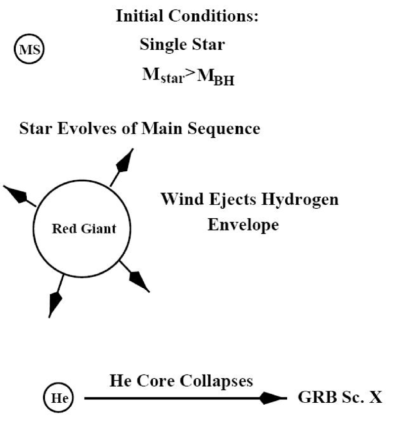
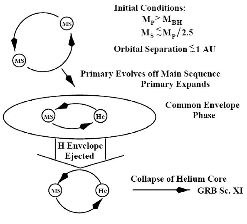
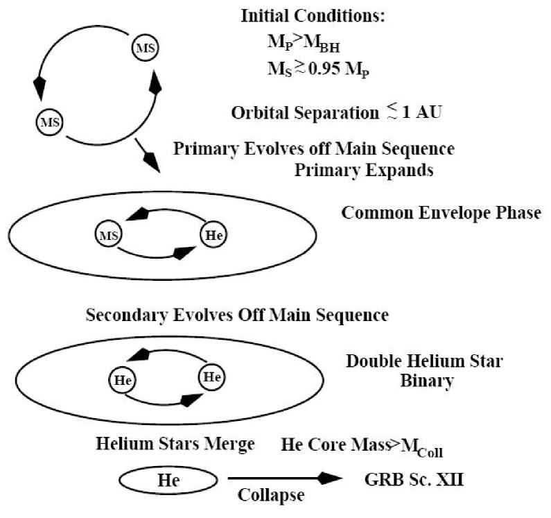
Figure 1.2: Three Scenarios A (upper left), B (upper right), C (lower figure) of collapsar formation proposed by Fryer, Woosley and Hartmann (1999).

1.3.2 Angular Momentum and Metallicity

The collapsar model requires an unusably large angular momentum in the inner regions of the massive progenitor stars lost their hydrogen envelope to from a disk around a black hole of several solar mass. The specific angular momentum

$$j=\frac{2GM}{3^{3/2}c}[1+2(3r_{lso}/r_{g}-2)^{1/2}]\simeq 10^{16}-10^{17}\rm cm^{2}\rm s^{-1}$$ (1.1)

where $M$ is the gravitational mass of the black hole, $r_{lso}$ is the radius of the last stable circular orbit, and $r_{g}=GM/c^{2}$. Wolf-Rayet (WR) stars with a very rapidly rotating core are good candidates for the progenitor. On the other hand, millisecond pulsars, which are more than one order of magnitude faster than he fastest observed pulsars, have a angular momentum $j\sim 10^{15}R_{10}^{-2}P_{1}^{-1}\rm cm^{2}\rm s^{-1}$ with $R_{10}=R/10^{7}$cm as the pulsar radius and $P_{1}=P/10^{-3}$s as the spin period. This angular momentum is still 1-2 orders of magnitude lower than the ones that make collapsars. Recent stellar evolution models which include angular momentum transport from the core to the hydrogen envelope by magnetic torques (Spruit 2002) lead naturally to rotation rates of pulsars in the range 10-15 ms, just what is needed for common pulsars result from the deaths of read supergiants (RSGs). However, the magnetic toques mechanism indicates the most single stars end up with cores rotate much slower than the ones in rapidly collapsars that lost their hydrogen envelopes. The problem is, if typical massive star death produces common pulsars, what special circumstance produce a GRB?

Magnetic torques are significant even when the envelope is removed. It coming from fields generated by the differential rotation have a tendency to enforce rigid rotation. Angular momentum is extracted from the inner core when it contracts and is transported to the outer layers which are spun up. Moreover, these magnetic torques brake the core when extensive mass loss slows down the rotation of the outer layers. Herger, Woosley & Spruit (2005) have found that magnetic torques decrease the final rotation rate of a collapsing iron core by about a factor of 30 ro 50. Furthermore, even without magnetic torques and even if the envelope of the star has been lost, the vigorous mass loss of typical WR stars still carries away lots of angular momentum. It has been known for some time that if the magnetic torques are negligible, which is to say much weaker than estimated by Spruit (2002), it is easy to give GRB progenitors the necessary angular momentum; but then one must invoke another mechanism to slow down from $10^{16}-10^{17}$ cm² s^-1 to typical pulsars with rotation period $\geq 15$ms.

Woolsey & Heger (2006) considered two ways to solve the problem. The first assumes that a fraction of WR stars have a mass loss which is not standard, for instance with a decrease of up to a long GRBs are produced at high redshift where the metallicity Z is much lower than in the solar system. Under these low metallicity conditions it is known that WR stars have a lower mass loss rate. The mass-loss rate of metal-deficient WR stars scales closer to $Z^{0.86}$. Another positive effect expected in WR stars with low metallicity is that they should rotate faster (Meynet & Maeder 2005). Finally, the mass loss anisotropies by stellar winds influence the loss of angular momentum. These anisotropies may result from mass-losses occurring predominantly at the poles, and help in reducing the loss of angular momentum because the loss of polar mass takes away less angular momentum than isotropic mass-loss. As a result, the GRB progenitors might be the few O and B stars with high rotational velocity ($\sim 400$km s${}^{-1})$ representing a few percent of this population. Moreover, because of the likely dependence of mass loss on metallicity, GRBs will be favored in regions of low metallicity. On the other hand, Yoon & Langer (2005) showed that the hydrogen envelopes retained due to the weakness of the stellar winds at low metallicity may not be a problem, because such low Z stars could become helium stars not by ejecting their hydrogen envelopes but burning the hydrogen into helium under through chemically homogeneous evolution. For low enough metallicity, this type of evolution can lead to retention of sufficient angular momentum in CO cores in the range from 10 $M_{\odot}$ to 40 $M_{\odot}$ to produce GRBs according to the collapsar scenario.

Both single-star models by Yoon & Langer (2005) and Woosley & Heger (2006) have made strong predictions about the low metallicity requirement of the progenitors. However, observations show that GRBs occur in environments with a range of metallicities from 1/100th solar to solar. The mean metallicity may be a high as 1/3-1/2 solar. Although we are unlikely to develop an observation technique that will permit a direct metallicity measurement of a GRB progenitor today, we are able to infer the metallicity of gas near the GRB progenitor by a few complementary approaches, for examples, by observing absorption line spectroscopy of GRB afterglows, or emission-line spectroscopy of H II regions within the GRB host galaxy (Fryer et al. 2007). The present set of metallicity measurements from $\approx$ 10 GRB afterglow spectra exhibit a large dispersion of values from $\approx 1/100$ solar (Chen et al. 2005) to nearly solar metallicity (Castro et al. 2003) with an average metallicity of 1/3-1/2 solar. These observations strong constraint on single-star models. In addition to the metallicity observation, the supernovae associated with GRBs that are bright enough to be studied in detail are almost Type Ic supernovae until now. If this result is universal, most progenitor model must lose not only its hydrogen envelope but most of its helium envelope as well. The single-star models, which produce He-rich (Type II) supernovae, do not fit the existing data of GRB-SN association as well. Furthermore, studying the progenitors of Type Ib/c sypernovae may also provide some insight into the progenitors of long GRBs. Evidence is growing that Type Ib/Ic supernovae preferentially occur in high-metallicity systems. Figure 1.3 shows the fraction of collapsing stars that form Type II and Tpe Ib/c supernovae as a function of metallicity (Heger et al. 2003). Note that single nonrotating stars produce Ib/c supernovae only at metallicities above 0.02 solar. But we expect these supernovae to have weak shocks and hence every very little nickel. Without the high shock temperature and the radioactive nickel to power the light curve, these supernovae will be dim. Strong Ib/Ic supernovae are not produced at all until the metallicity rises above solar! This conclusion could also be maintained for rapidly rotating stars. As a result, the above mentioned argues strongly show that the single-star models at low metallicity, cannot explain all the long bursts. As the date get better, the limitations on single-star models will become more strict.

Figure 1.3: Single-star supernova rate as a fraction of total number of collapsing stars as a function of metallicity calculated using the stellar models (Heger et al. 2003; Fryer et al. 2007). Three classes of Type II SNe in this figure include normal Type II SNe (Type II), Type II SNe with weak SN explosions (Type II weak), and Type II SNe that have lost most of their hydrogen envelope (Type IIL); and two classes of Type Ib/c SNe are normal Ib/c SNe and weak Ib/c SNe. If single stars dominate the Ib/c rate, these models predict only weak Type Ib/c SNe below solar metallicity.

Scenario	Angular Momentum	Metallicity Trend	Surrounding	Associated Supernovae
			Environment
Classic single	Low?	Rate peaks $\sim 0.1Z_{\odot}$	High wind, Low wind	H-rich to He-rich
Mixing single	Good	$Z<0.1Z_{\odot}$	Low wind	All He-rich
Classic binary	Low?	Rate$\uparrow$ $Z\downarrow$	Tends to low wind	He-rich, He-poor
Tidal binary	Good?	Rate$\uparrow$ $Z\downarrow$	Tends to low wind	He-rich, He-poor
Brown merger	Good?	Rate$\uparrow$ $Z\downarrow$	Tends to low wind	He-rich, He-poor
Explosive ejection	Good?	Rate$\uparrow$ $Z\downarrow$	Shell within 1 pc	He-poor
He merger	High	Rate$\uparrow$ $Z\downarrow$	Tends to low wind	He-rich, He-poor
He case C	Good?	Rate$\uparrow$ $Z\downarrow$	Tends to low wind	He-rich, more He-poor
Cluster	Good?	Rate$\uparrow$ $Z\downarrow$	Tends to low wind	He-rich?

Table 1.3: Different scenarios of collapsar progenitors (Fryer et al. 2007)

Therefore, we should also consider binary systems as the long GRB progenitors, as suggested by Fryer et al. (1999). For many binary progenitor models, the binary component is used to remove the hydrogen envelope without the angular momentum loss that occurs in wind mass loss. Also, the binary models tend to fit the metallicity constraints well. Several binary progenitors can match the solid observational constraints and also have the potential to match the trends that we are currently seeing the observations mentioned above. Table 1.3 is the list of all the progenitors studied and their basic predictions from Fryer et al. (2007).

1.3.3 Jet Formation, Propagation and Breakout

In collapsing massive stars, as a consequence of the in-fall into the black hole of the matter which was initially situated along the rotational axis and of the stagnation of matter in the equatorial disk, a favorable geometry for jet outflow develops. Energy is dissipated in the disk around a black hole by neutron annihilation or MHD processes such as Blandford-Znajek (BZ) process, which can power polar outflows, relativistically expanding bubbles of radiation, and pairs and baryons focused by density and pressure gradients into jets.

McFadyen & Woosley (1999) showed that for a reasonable but optimistic values, the total neutrino energy emitted by the disk during 20s of accretion process is $3\times 10^{53}$ ergs, and the total energy deposited by neutrino annihilation was $1.4\times 10^{52}$ ergs. For less optimistic assumptions regarding, the initial Kerr parameter and the neutrino transport, the emitted energy was as low as $1.4\times 10^{53}$ ergs and the deposited energy $\leq 1\times 10^{51}$ ergs. But these numbers are obtained for the particular model considered by the authors. A typical factor-of-10 uncertainty can be due to the sensitivity of the model to the accretion rate and to the Kerr parameter characterizing the initial angular momentum of the black hole, but also to the uncertainty in the neutrino efficiencies. The neutrino annihilation efficiencies will be discussed in §2.7. more detailed. Anyway, after a fraction of a second, the energy to mass ration in these jets became very large $\leq 10^{22}$ ergs s^-1, corresponding to a large asymptotic relativistic Lorentz factor. The problem of "baryonic contamination" is circumvented because the energy deposition blows a bubble of low density. Momentum and energy from the annihilating neutrinos continues to be deposited in this bubble even as the baryon fraction becomes small. The pressure gradient in the bubble has a component pointing away from the polar axis that tends to exclude gas from the polar region. This energy is naturally directed outward along the axis. However, lacking a full special relativistic calculation of the entire event, the jet propagation cannot be accurately determined in MacFadyen & Woosley (1999).

The propagation of relativistic jet through the collapsing rotating massive star were studied by Aloy et al. (2000), Zhang et al. (2003, 2004). They did not discuss how jet form during the collapse process, but focus on its propagation. Aloy et al. (1999) have recalculated the 14 $M_{\odot}$ collapsar model of MacFadyen & Woosley, using a 3-D and fully relativistic code. The relativistic jet forms as a consequence of an assumed energy deposition ($10^{50}-10^{51}$ ergs s^-1) within a $30^{\circ}$ cone around the rotation axis. The jet flow is strongly beamed (few degrees) spatially inhomogeneous and time-dependent. The jet is able to reach the surface of the stellar progenitor (typically $R\sim 3\times 10^{10}$ cm) intact. At breakout, the Lorentz factor of the jet reaches $\Gamma\sim 33$. After breakout the jet accelerates into the circumstellar medium, whose density is assumed to decrease exponentially and then become constant, $\rho_{\rm ext}=10^{-5}$ g cm^-3. Outside the star, the flow begins to expand laterally also ($v\sim c$), but the beam remains very well collimated. At a distance of 2.54 $R_{*}$, where the simulation ends, about 2s after shock breakout, the Lorentz factor has increased to $\Gamma$=44 in the core of the jet which is now highly collimated ($\sim 1^{\circ}$). At that time the jet has reached $7.5\times 10^{10}$ cm, which is $10^{2}$ to $10^{4}$ smaller than the distance at which the fireball becomes optically thin. and the values of Lorentz factor $\Gamma$ are still far from those required for the fireball model.

Zhang, Woosley & MacFadyen (2003) and Zhang, Woosley & Heger (2004) go farther in the jet-stellar envelope interaction simulations. While the simulation stops when the bulk Lorentz factor $\Gamma$ reaches 44 in the work of Aloy et al. (2000), Zhang, Woosley & MacFadyen (2003) picked up the calculation when the jet, which presumably began in a region $\sim 30$ km in size, has already reaches a radius of 2000 km and do not consider what has gone on inside. Each jet is parameterized by a radius where it is introduced and by its initial Lorentz factor, opening angle, power, and internal energy. In agreement with Aloy et al. (2000), Zhang, Woosley & MacFadyen (2003) found that relativistic jets are collimated by their passage through the stellar mantle. Starting with an initial half-angle of up to $20^{\circ}$, they emerge with half-angles that, though variable with time, are around $5^{\circ}$. Interaction of these jets with the star and their own cocoons also causes mixing that sporadically decelerates the flow. The mixing instabilities along the beams surface is chiefly responsible for the variable Lorentz factor needed in the internal shock model and for the complex light arrives in many GRBs. Moreover, the jet is shocked deep inside the star following a brief period of adiabatic expansion; and this shock converts most of the jet’s kinetic energy into internal energy. Eventually, the jet accelerates and breaks free of the star with very large internal energy. Conversion of the remaining internal energy gives terminal Lorentz factors along the axis of $\sim 100-200$. Table 1.4 list the jet models of Zhang, Woosley & MacFayden (2003) with different initial parameters. Jet propagations is studied in two steps. inside the star and in the stellar wind environment after breakout. Both steps the jet is specified by six parameters as shown in Table 1.4. Figure 1.4 and Figure 1.5show the selected calculation results (JA & W1) of bulk Lorentz factor from these models.

Model	$\dot{E}^{a}$	$\theta_{0}^{b}$	$\Gamma_{0}^{c}$	$f_{0}^{d}$
	($\times 10^{51}$ ergs s-1)	(deg)
JA	1.0	20	50	0.33
JB	1.0	5	50	0.33
JC	0.3	10	5	0.025
W1	0.8	3	10	0.06
W2	0.8	3	50	0.33

Table 1.4: Parameterized initial conditions for jet propagation inside a star from radius $\approx 2000$ km (JA, JB, JC) and in the stellar wind after breakout (W1, W2) from Zhang, Woosley & MacFayden (1999): ^a Energy deposition rate for each jet; ^b Initial half-angle; ^c Initial Lorentz factor; ^d Initial ratio of kinetic energy to total energy, which excludes the rest mass. They did not consider the process of jet formation

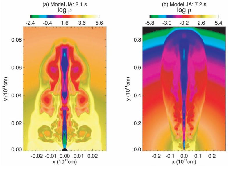
Figure 1.4: Density structure in the local rest frame for model JA at (a) t=2.1 s and (b) 7.2 s. In (a), only the central region of the star is shown. The radius of the star is $8\times 10^{10}$ cm (Zhang, Woosley, MacFadyen 2003).

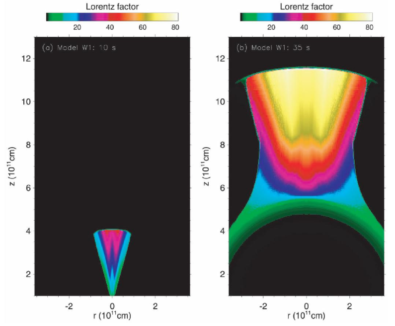
Figure 1.5: Bulk Lorentz factor for model W1 at (a) t=10 s and (b) t=35 s after the jets start to propagate in the stellar wind. The initial opening angle is 3^∘. At t=35 s, the opening angle is $\sim 15^{\circ}$. Because the power and Lorentz factor decrease gradually after 10 s, the tail of the jet has much more lateral expansion (Zhang, Woosley, MacFadyen 2003).

Because of the large radio of internal to kinetic energy in both the jet ($\geq 80\%$) and its cocoon, the opening angle of the final jets after breakout is significant greater than at breakout. Figure 1.5 is an example of Lorentz factor at t=10 and t=35 after the jets break out of the star and propagate in the star wind. A small amount of material emerges at large angles, with a Lorentz factor still sufficiently large to make a weak GRB. This suggests a unified scenario which can explain various types of high-energy transients from X-ray flashes to classic GRBs, depending on the angle at which at standard collapsar is observed. Later Zhang, Woosley & Heger (2004) used new 2-D and 3-D simulations to further studied the relativistic jet propagation and breakout in massive WR stars and improved their former results. The highly relativistic jets are ($3^{\circ}-5^{\circ}$, $\Gamma\geq 100$) is surrounded by a cocoon with moderately relativistic ejecta ($\Gamma\sim 15$) that expands and become visible at large polar angles ($\sim 10^{\circ}$). As a results, XRFs and GRBs should be different expressions of the sam basic phenomenon from collapsars.

Another way to produced $\gamma$-ray and X-ray transients related with cocoon was proposed by Mészáros & Rees (2001) and Ramirez-Ruiz, Celotti & Rees (2002). Most of the energy output during the period that the jet through the stellar core goes in a cocoon of relativistic plasma surrounding the jet. This cocoon material subsequently forms a bubble of magnetized plasma that takes several hours to expand, subrelativistically, through the envelope of a massive star. Mészáros & Rees (2001) showed that the shock waves and magnetic dissipation in the escaping bubble can contribute a nonthermal UV/X-ray afterglow, and also excite Fe line emission from thermal gas, in additional to the standard jet deceleration power-law afterglow. Ramirez-Ruiz et al. (2002) also discussed that a rebrightening caused by the cocoon photospheric emission might appear with energy greater than $10^{50}$ ergs. If the relativistic jet cames less energy and inertia than the cocoon plasma itself, it will start to decelerate at a smaller radius than the collimated cocoon fireball, and the afterglow would be dominated by the emission of the cocoon material. On the other hand, if the jet produced by the accretion maintains its energy for much longer than it takes the jet head to reach the surface of the helium envelope, the relativistic jet is likely to contain substantially more energy than the off-axis cocoon material.

Besides jet and cocoon’s propagation and breakout, in Nagataki et al. (2007) and Nagataki (2009), jet formation process in collapsars is studied. Nagataki et al. (2007) investigated the dynamics of collapsar using 2-D MHD simulations (Newtonian ZEUS-2D code) that generates a jet, taking account of realistic equation of state (contribution of electrons, positrons, radiation and ideal gas of nuclei), neutrino cooling and heating processes, magnetic fields, and gravitational force from the central black hole and self-gravity. It is founded that neutrino heating processes ($\nu\bar{\nu}$ pair annihilation and $\nu_{e}\bar{\nu}_{e}$ captures on free nucleons) are not so efficient to launch a jet in the Newtonian scenario. On the other hand, a jet could be launched by $B_{\phi}$ fields that are amplified by the winding-up effect. However, Tagataki et al. (2007) showed that the radio of total energy relative to the rest mass energy in the jet at the final stage of simulations suggest the bulk Lorentz factor of the jet $\Gamma$ will not reach to as several hundreds, therefore the jet will not be a GRB jet. Later Tagataki (2009) developed a 2-D general relativistic MHD (GRMHD) code to further investigate the formation of relativistic jets from a collapsar. He adopted a model from Woosley & Heger (2006), which corresponds to a 12 $M_{\odot}$ star initially with 1% of solar metallicity and relatively large iron core of 1.82 $M_{\odot}$. Effects of magnetic fields are taken into account with the vector potential $A_{\phi}\propto{\rm max}(\rho/\rho_{\rm max}-0.2,0)\textrm{sin}^{4}\theta$, where $\rho_{\rm max}$ is the peak density in the progenitor. This magnetic structure is initially introduced in Fishbone-Moncrief’s solution with magnetic fields (Gammie et al. 2003). On the other hand, he did not consider the neutrino emission and heating processes. Based on these considerations, it is shown that a jet is launched from the center of the progenitor. Figure 1.6 shows the contours of the plasma $\beta$($=p_{gas}/p_{mag}$) in logarithms scale at $t=1.773$ s. The plasma $\beta$ is low in the jet region but high in the accretion disk region. The jet is a Poynting flux jet surrounded by a funnel-wall jet.

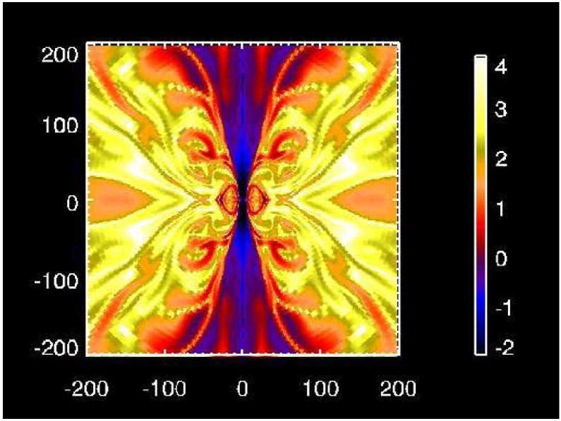
Figure 1.6: Contour of the plasma $\beta$ ($p_{gas}/p_{mag}$) at t = 1.773 s in logarithmic scale (Nagataki 2009).

However, even at the final stage of the simulation with a time evolution of 1.773 s, the bulk Lorentz factor of the jet is still low, and the total energy of the jet is as small as $\sim 10^{48}$ ergs. Since the energy flux per unit rest-mass flux is $\sim 100$ at the bottom of the jet, Tagataki (2009) suggested it is still possible the jet Lorentz factor to be high enough when it propagates outwards. Also, a long duration of the collapsar activity could still make the total energy of jet large enough to $\sim 10^{50}-10^{51}$ ergs. Moreover, in this GRMHD simulations, jet is launched mainly by the magnetic field amplified by the gravitational collapse and differential rotation around the black hole, rather than the Blandford-Znajek mechanism. Therefore, more detailed simulations with a time evolution $\sim 10$ s should be operated for determining the jet formation scenario. On the other hand, it is interesting to describe the collapsar model as an entire consistent scenario from the progenitor to the jet and cocoon breakout. What is the role played by magnetic fields in angular momentum transportation and jet formation and propagation? As Tagataki (2009) studied Poynting flux jet rather than baryonic jet, it is still interesting to simulate the propagation of such magnetized jets.

1.3.4 GRB-SNe Association

GRB-SN (XRF-SN) association greatly show the linking between the GRBs and the collapse of massive stars in star formation regions. Woosley & Bloom (2006) reviewed the evidence for and theoretical implications of this assocation detailed. As GRB-SN association is one of the key evidence to support the collapsar model, I also give a brief review in this section.

There are at least five examples of GRB-SN or XRF-SN association had been confirmed spectroscopically. Table 1.5 gives the properties of these GRB(XRF)-SN events. The first case of GRB-SN association was GRB 980425, which has been associated with SN 1998 bw.

GRB/SN	$z$	Eiso($\gamma$)	ESN	M(56Ni)	SN type	References
		($10^{49}$ ergs)	($10^{52}$ ergs)	($M_{\odot}$)
980425/1998bw	0.0085	0.06-0.08	2-3	0.5-0.7	Ic-BL	Iwamoto et al. (1998)
030329/2003dh	0.1685	1070	2-5	0.3-0.55	Ic-BL	Stanek et al. (2003), Mazzali et al. (2003), etc
031203/2003lw	0.1005	2.94$\pm$0.11	2-3	0.5-0.7	Ibc-BL	Malesani et al. (2004), Gal-Yam et al. (2004), etc.
060218/2006aj	0.0335	5.9$\pm$0.3	0.025	0.2$\pm$0.04	Ic	Soderberg et al. (2006b), Mazzali et al. (2006)
080109/2008D	0.00649	$\sim 0.002$	0.3-0.6	0.05-0.1	Ib	Soderberg et al. (2008), Mazzali et al. (2008)

Table 1.5: Physical Properties of confirmed GRB-SNe association events up to 2008.

GRB 980425 triggered detectors on broad both BeppoSAX and BATSE (Kippen, 1998). At high energies, it was seemingly unremarkable (Kippen 1998; Galama et al. 1998) with a typical soft spectrum ($E_{\rm peak}\approx 150$keV) and moderate duration ($\triangle T\approx$23 s). GRB 980425 arose from the redshift $z=0.085$ galaxy, and has $R_{\gamma,\rm iso}=8.5\pm 0.1\times 10^{47}$ ergs if assuming isotropic emission. This energy is more than three orders of magnitude fainter than the majority of long-duration GRBs. Any collimation would imply an even smaller energy release in GRBs. The evolution of SN 1998bw was unusually at all wavelengths. The discovery of prompt radio emission just a few days after the GRB (Kulkarni et al. 1998, see Figure ** in detail) was novel. Almost irrespective of modeling assumptions, the rapid rise of radio emission from SN 1998bw showed that the time of the SN explosion was the same as the GRB to about one day. The brightness temperature several days after the GRB suggested the radio photosphere moved relativistically with $\Gamma\geq 3$. The total supernova kinetic energy is as large as $\sim 2-5\times 10^{52}$ ergs more than ten times the previous know energy of supernova. So the explosion is called a ’hypernova’. Such a C+O star is the stripped core of a very massive star that has lost both of its hydrogen and helium envelopes.

The first truly solid evidence for a association between ordinary GRBs and SNe came with the detection of the low-redshift ($z=0.1685$, Greiner et al. 2003) GRB 030329 and its associated supernova, SN 2003dh. Shortly after its discovery (the brightest burst HETE-2 ever saw), the afterglow of the GRB was very bright ($R\sim 13$mag). If faded slowly, undergoing several major rebrightening events in the first few days (Burenin et al., 2003; Greiner et al. 2003, etc.). Given the low redshift, several spectroscopic campaigns were initiated. Spectra of the afterglow, 6.6 and 7.7 days after the GRB, showed a deviation from a pure power-law and the mergence of broad SN spectral feature.

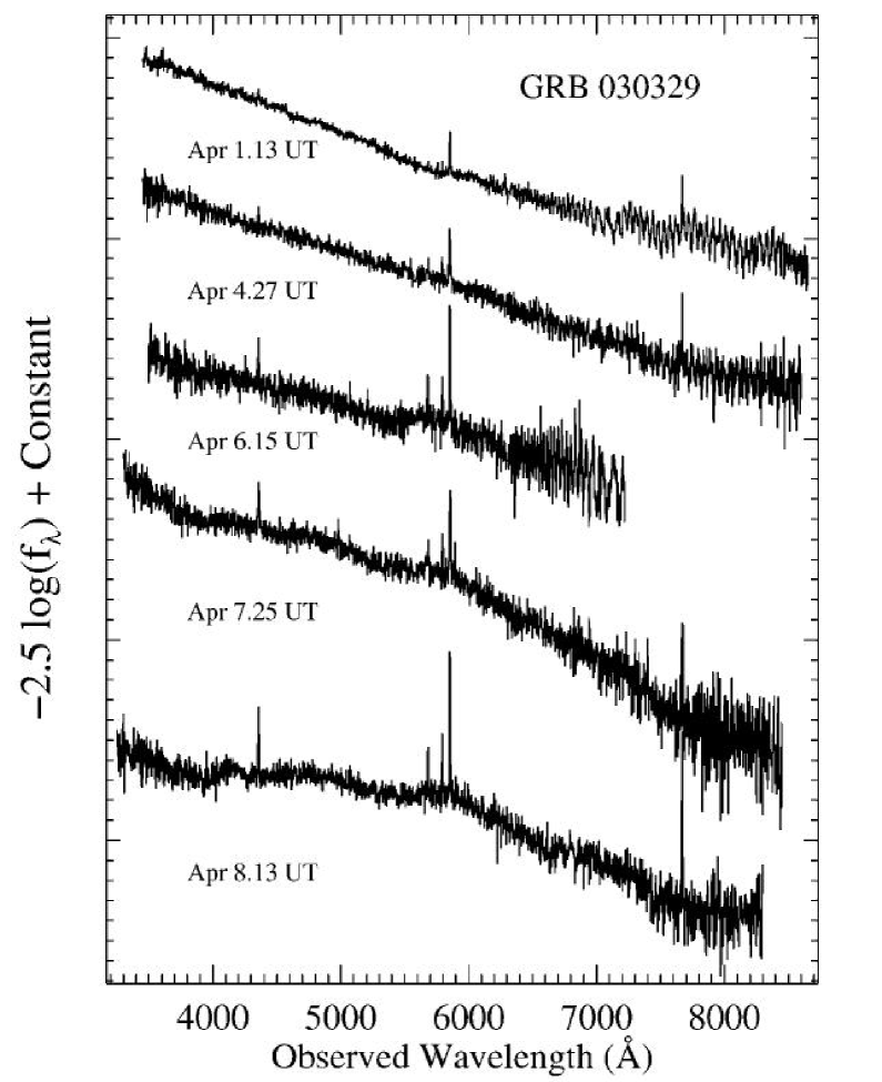
Figure 1.7: 1.Evolution of the GRB 03029/SN 2003 spectrum, from April 1.13 UT (2.64 days after the burst) to April 8.13 UT (9.64 days after the burst). The early spectra consist of a power-law continuum with narrow emission lines originating from H II regions in the host galaxy at a $z=0.168$. Spectra taken after April 5 show the development of broad peaks in the spectra characteristic of a supernova (Stanek et al. 2003).

Figure 1.7 shows the evolution of the GRB 030329/Sn 2003dh spectrum from Stanek et al. (2003). Spectrapolarimetric observations at later times showed that the SN light was somewhat polarized ($P<1\%$) indicating mild asymmetry in the subrelativistic ejecta. Given the broad spectral features, indicating high velocities ($\geq 250000$km s^-1; Stanek et al. 2003), and apparent absence of hydrogen, helium and strong Si II $\lambda$6355 absorption, a classification as Type Ic-BL was natural.

The association of XRF 080109 with SN 2008D is the first GRB-SN event which shows a Type Ib supernova. The unabsorbed peak X-ray luminosity of XRF 080109 (or called X-ray outburst by Soderberg et al. 2008) is $L_{X,p}\approx 6.1\times 10^{43}$ergs s^-1 which the fluence is $f_{X}\approx 2\times 10^{46}$ergs (Soderberg et al. 2008). The peak luminosity of the XRF(XRO) is about 2 orders of magnitude brighter than ULX outbursts, and about 3 orders of magnitude brighter than Type I X-ray bursts, which additionally have blackbody spectra. In comparison to other GRBs/XRFs, the value of $E_{X}$ is about three orders of magnitude lower. Therefore, the properties of XRF 080109 are distinct from those of all know X-ray transients. These properties can be explained as the breakout of the supernova shock through a dense wind surrounding the compact ($\sim 10^{11}$ cm) progenitor star. Moreover, SN 2008D also showed several unusual features including (i) an early narrow optical peak (ii) disappearance of the broad lines typical of SN Ic hypernovae and (iii) development of helium lines as in SN Ib (Mazzali et al. 2008). Detailed analysis shows that SN 2008D was not a normal supernova. Its explosion energy $E\approx 6\times 10^{51}$ergs and ejected mass $\sim 7M_{\odot}$ are intermediate between normal SNe Ibc and hypernovae. SN 2008D is probably among the weakest explosions that produce relativistic jets.

Besides the above examples showed in Table 1.5, there are other GRBs whose late-time deviations from the power-law decline typically observed for optical afterglows have been seen in a number of cases, and these bumps in the light curves have been interpreted as evidence of supernovae. A report of a red emission "bump" following GRB 980326 (Bloom & Kulkarni, 1999), was interpreted as due to a coincident SN at about a redshift of unity (see Figure 1.8).

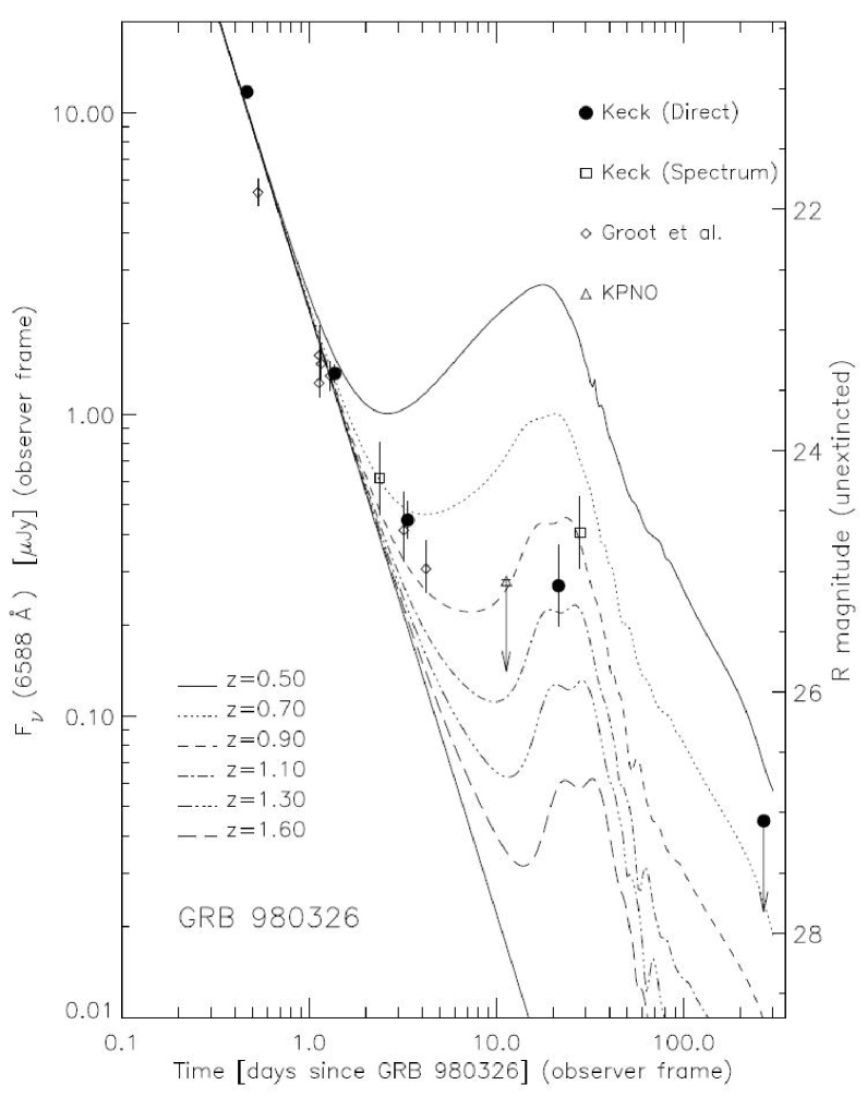
Figure 1.8: An "optical bump" on the afterglow of GRB 980326 (Bloom et al. 1999). Models of SN 1998 bw at different redshifts are shown.

Without a spectroscopic redshift for GRB 980326 and multi-band photometry around the peak of the bump, the absolute peak brightness and type of the purported SN could not be known. The available date were also consistent with a dust echo (Esin & Blandford, 2000), or dust re-radiation (Waxman & Draine, 2000) from material surrounding the GRB. A subsequent reanalysis of the afterglow of GRB 970228 revealed evidence for a bump which appeared to be the same absolute magnitude as SN 1998bw with similar rise time (Reichart, 1999; Galama et al. 2000). Similar reports of bumps were made (Sahu et al., 2000; Frucher et al., 2000; Björnsson et al., 2001; Lazzati et al., 2001; Castro-Tirado et al., 2001; Sokolov, 2001; Berger et al., 2001; Gorosabel et al., 2005; Masetti et al., 2005), but mone as significant and with as clear cut association to SNe as GRB 980326 and GRB 970228.

Concerted multi-epoch ground-based and space-based observing campaigns following several GRBs strengthened the notation that late-time bumps were indeed SNe. For example, the SN 0f GRB 011121 showed a spectral rollover during peak around 4000Å, nominally expected of core-collapse SNe in the photospheric phase. Garnavich et al. (2003) showed evidence that the brightness and color evolution resembled 1998S and Type IIn; on the other hand, Bloom et al. (2002) showed consistency with a Ic-like curve interpolated between the faint and fast 1994I and the bright and slow 1998bw. Zeh et al. (2004) published an important photometric study of bumps in GRBs, fitting 21 of the best sampled afterglows and finding evidence of 9 bumps. Statistically significant evidence for bumps are found in 4 GRB afterglows (990712, 991208, 011121, and 020405) while 5 have marginal significance (970228, 980703, 000911, 010921, and 021211). All of these GRBs had bumps claimed prior to the Zeh analysis. Zeh et al. (2004) emphasize that all GRBs with $z\leq 0.7$ appear to have bumps, which of course, would be expected if all long-duration GRBs have associated SNe. However, bump detection does not necessarily imply a SN detection. There are, in fact, important cases where multi-band photometry has curves of GRB990712 and XRF 030723, for example, do not appear consistent with a supernova. Table 1.6 shows the properties of good candidate supernovae associated with GRBs, XRFs and XRR (X-ray rich GRBs) up to 2005.

GRB/SN	$z$	Peak	$T^{a}_{\rm peak}$	SN likeness	References
		[mag]	[day]	designation)
XRF 020903	0.25	$M_{V}=-18.6\pm 0.5$	$\sim 15$	Ic-BL	Soderberg et al. (2005)
GRB 011121/2001dk	0.365	$M_{V}$=-18.5 to -19.6	12-14	I(IIn?)	Bloom et al. (2002), etc.
GRB 050525a	0.606	$M_{V}\approx-18.8$	12	I	Della Valle et al. (2006)
GRB 021211/2002lt	1.00	$M_{V}=-18.4$ to -19.2	$\sim 14$	Ic	Della Valle et al. (2004)
GRB 970228	0.695	$M_{V}\sim-19.2$	$\sim 17$	I	Galama et al. (2000)
XRR 041006	0.716	$M_{V}=$-18.8 to -19.5	16-20	I	Stanek et al. (2005), etc.
XRR 040924	0.859	$M_{V}=-17.6$	$\sim 11$	I	Soderberg et al. (2006a)
GRB 020405	0.695	$M_{V}\sim-18.7$	$\sim 17$	I	Price et al. (2003)

Table 1.6: Properties of good candidate SNe associated with GRBs, X-Ray Flashes, and X-Ray Rich GRBs, up to mid 2005 (Woosley & Bloom 2006).

The collapsar model suggested the supernova and the GRB derive their energies from different sources. The supernova, and the ⁵⁶Ni to make it bright, are produced by a disk "wind" (MacFadyen & Woosley, 1999; Kohri et al. 2005). This wind is subrelativistic with a speed comparable to the escape velocity of the inner disk, or about 0.1c. On the other hand, Nagataki et al. (2006) studied that ⁵⁶Ni produced in the jet of the collapsar is not sufficiently to explain the observed amount of a hypernova when the duration of the explosion is $\sim$10 s, which is considered to be the typical timescale of explosion in the collapsar model. This result also suggest that the sufficient ⁵⁶Ni is provided from the accretion disk outflow.

We should keep in mind there are at least some GRBs do not have associated supernovae. Woosley & Bloom (2006) discussed some extrinsic biases which against detecting the associated SNe: for example, poor localizations of bursts from their afterglows dramatically hamper the ability for large aperture telescope to discover emerging SNe; fainter SNe are expected from bursts that occur near the line-of-sight through the Galaxy, or in especially extinction-riddled regions of their host, which diminished the sensitivity of the supernova observations; the host galaxies of GRBs may still contaminate the light of GRB SNe at late times. However, Fynbo et al. (2006) and Watson et al. (2007) discussed that no supernova emission associated the two nearby long-duration bursts 060505 at $z$=0.089 and 060614 at $z$=0.125, otherwise the associated supernovae should down to limits hundered of times fainter than the archetypal SN 1998bw, and fainter than any type Ic SN ever observed. Since the luminosity of a SN is roughly proportional to the total amount of ⁵⁶Ni produced in the explosion it would mean that some GRBs produced very little ⁵⁶Ni ($<0.007M_{\odot}$). This would be explained as the case for Type II collapsar (Fryer, Young, & Hungerford 2006); or it is possible that such GRBs without SNe are from low-mass, long-lived progenitors which might be similar to those producing short GRBs.

1.4 Progenitor II: Merges of Compact Stars

1.4.1 Binary Evolution and Mergers Rate

Mergers of compact objects as the sources of short-hard GRBs have been studied for years (Paczynski 1986, 1990; Eichler et al. 1989). In the collapsar model, which is a good candidate for long-duration GRBs, a spinning black hole with a accretion disk is formed. Mergers of compact objects can also lead to the formation of a stellar-mass black hole. The black hole would be unable to swallow the large amount of angular momentum present in the binary system. The debris from the tidally disrupted compact object forms a transient accretion disk or tours, and ultimately falls into the black hole and release a fraction of the gravitational binding energy. This hyperaccreting disk scenario is similar to the central engine suggested for long GRBs, and naturally explain the similarity between these two phenomena.

Compact objects related to short-hard GRBs can be classified to several types: neutron stars (NS-NS) mergers, black hole-neutron star (BH-NS) mergers, black hole helium star (BH-He) mergers, black hole white dwarf (BH-WD) mergers and merging white dwarfs binary (WD-WD). The binaries formation scenario always begins with two massive stars, which evolve to different types of binaries. Here we provides various scenarios for forming NS/NS, BH/NS and BH/He based on the review by Fryer, Woosley & Hartmann (1999).

NS/NS Scenarios

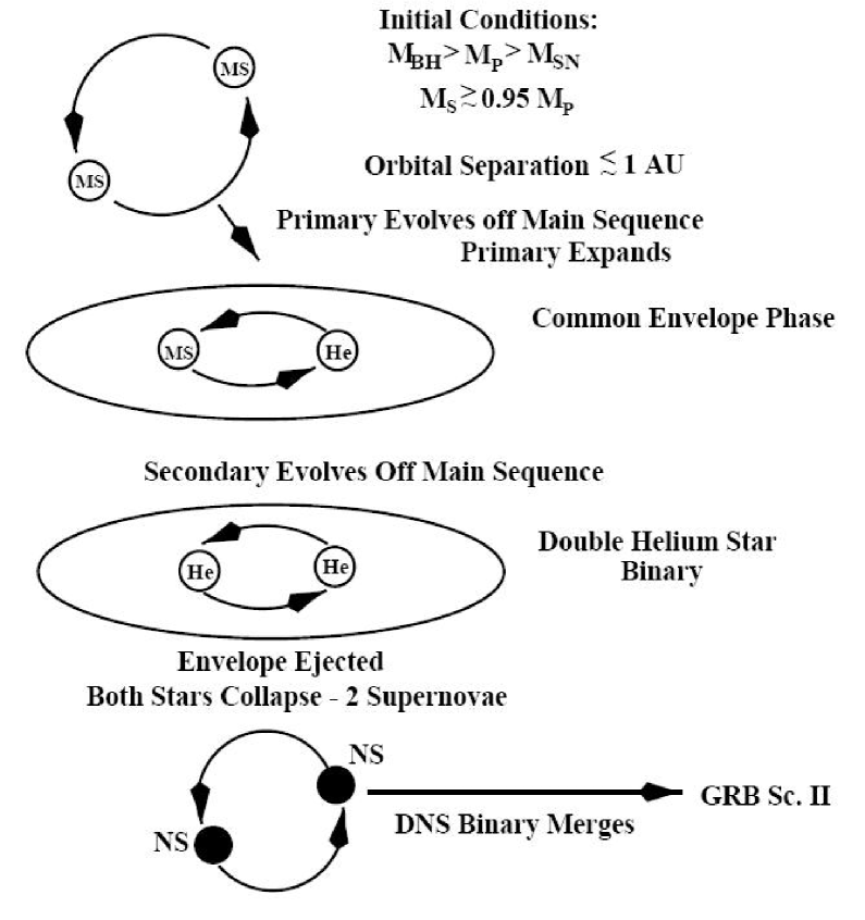
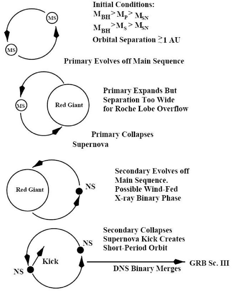
Figure 1.9: Two Scenarios NS/NS-b, NS/NS-c for neutron star binary formation from Fryer, Woosley and Hartmann (1999). Scenario NS/NS-a, which evolves through the common envelope phase, is unlike to form NS/NS binary system (Bethe & Brown 1998).

• Scenario NS/NS-a: "Standard" double NS formation scenario. The more massive star (primary) evolves off the main sequence, overfills its Roche lobe, and transfers mass to its companions. The primary then evolves to the end of its life, forms a NS in a SN explosion. Next this system passes through an X-ray binary phase, which then evolves through a common envelops phases in the standard model. The neutron star spirals into the massive companion and forms a NS/BH binary, which finally evolves to a close NS/NS binary, after the explosion of the helium star.

  However, farther calculations reveal that, during the common envelope phase, the NS accretes at the Bondi-Hoyle rate and collapse to form a black hole (Chevalier 1993, 1996; Brown 1995; Bethe & Brown 1998; etc.). As a result, this "standard" scenario for NS/Ns systems may in fact form BH/NS binaries.

• Scenario NS/NS-b: "Brown" mechanism for NS/NS binaries (Brwon 1995). The initial binary system is comprised of two massive stars of nearly equal mass. The secondary evolves off the main sequence before the explosion of the primary as a supernova. The two stars then enter a common envelope phase with two helium cores orbiting within one combined hydrogen envelope. After the hydrogen envelope is ejected, first one helium star, then the other, explodes. if the kicks kicks imparted to the NSs during the supernova explosion do not disrupt the binary, a NS/SN system can form.

• Scenario NS/NS-c: Kick scenario for double NS binaries. The system avoids any common envelope phase but requires that the NS formed in the explosion of the secondary receive a kick that places it into an orbit that will allow the two NSs to merge within a Hubble time. However, to aviod a common envelope phase, the presupernova orbital separation must be $>1AU$. The range of kick magnitudes and directions that will produce a small orbit. This case is probably rare compared to other scenarios.

Figure 1.9 shows the scenarios to form NS/NS binary systems.

BH/NS Scenarios

• Scenario BH/NS-a: "Standard" BH/NS binary formation scenario. The primary, with a mass greater than the limit for black hole from fallback $M_{\rm BH}\approx 25M_{\odot}$, evolves off the main sequence, overfill its Roche lobe, and transfers mass to its companion. After the end of its life, the primary forms a BH, and possibly, a supernova explosion. Then a binary consisting of a BH and a massive star passes through an X-ray binary phase if this system does not suffer from large kicks. Next the binary system evolves through a common envelope, and the BH spiral into the massive secondary and ejects the secondary’s hydrogen envelope. The BH/NS binary finally forms after the secondary’s supernova explosion.

• Scenario BH/NS-b: This scenario is similar to the NS/NS-a scenario. The neutron star gains too much matter during common envelop phase and collapses into a BH. This formation scenario produces a binary consisting of a low-mass BH ($\sim 3M_{\odot}$) and a NS.

• Scenario BH/NS-c: Kick scenario for BH/NS binaries. Just as with the NS/NS system, a BH/NS binary can form under a third mechanism, avoiding any common envelope evolution for appropriate kick magnitudes and directions. However, as the NS/NS kick formation scenario, the probability of this kick scenario is somewhat rare.

BH/WD Scenarios

• As WD/BH binary merge, the white dwarf is tidally disrupted and most of its matter is converted into an accretion disk around the BH. The accretion of this disk matter onto the BH may drive a GRB. The energy from neutrino annihilation process is negligible for most cases in WD-BH megers (Popham et al. 1999). The timescale of accretion for disk formed in BH-WD mergers is in the range of long-duration GRBs, but the rate of BH-WD merger is even lower than NS-NS and BH-NS mergers. Therefore, BH/WD mergers are not likely to be the leading causes of most GRBs. BH/WD binary may begin with a binary consisting of a primary with mass great than $M_{\rm BH}$ mentioned above and a low-mass ($<10M_{\odot}$) companion, or it can also from neutron star system with low-mass ($<10M_{\odot}$) companions scenario.

Table 1.7 provides a list of various rate estimates for some of these possible short-hard GRBs progenitors based on the review Lee & Ramirez-Ruiz (2007), and compared them to the rate of SNe events. However, there are many factors to cause the uncertain of these rates, such as the supernova kicks, the mass ratio distribution in binaries, mass limit for BH formation, stellar radii and common envelope evolution and so on (e.g. Fryer et al. 1999; Clark et al. 1979; Lipunov et al. 1987; Phinney 1991; Tutukov e& Yungelson 1993; Lipunov et al. 1995; Bloom et al. 1999; Belczynski et al. 2001, 2002, 2006).

Progenitor	Rate ($z=0$)
NS-NS	1-800
BH-NS	0.1-1000
BH-WD	0.01-1000
BH-He	$\sim 1000$
NS AIC	0.1-100
WD-WD	3000
SN Ib/c	60000
SN Ia	150000
SGRBs	10(4$\pi/\Omega$)

Table 1.7: Estimated progenitors of SGRBs and their plausible rates in yr^-1 Gpc^-3. The rates for these various occurrences are plauged by a variety of uncertainties in many aspects. The observed rates of Type (Ia+Ib/c) events given here provide a generous upper limit (Lee & Ramirez-Ruiz, 2007).

The mergers rate and typical lifetime of NS/NS binaries are estimated based on the observed system in our Galaxy or theoretical population synthesis. The current detection of NS/NS binaries in our Galaxy depends on at least one of the companions being a recycle pulsar. The sample of observed NS/NS binaries is still small today. We have only three NS/NS binaries examples: PRS B1913+16, PSR B1934+12 and PSR J0737-3039. The first calculations of the Galactic NS-NS merger rate, which were based on two systems (PRS B1913+16 & PSR B1934+12), showed the rate is between $10^{-6}$ to $10^{-5}$ per yr per galaxy (Phinney 1991; Narayan, Piran & Shemi 1991). The discovery of the relativistic third binary pulsar PSR J0737-3039 makes the Galactic mergers rate increased to $1.7\times 10^{-5}-2.9\times 10^{-4}$yr^-1 at 95% confidence and the local universe mergers rate to be 200-3000 Gpc^-3 yr^-1 (Kalogera et al. 2004). On the other hand, population synthesis showed the NS-NS mergers rate span over two orders of magnitude, which include the range inferred from observed Galactic binaries. Bethe & Brown (1998) suggested that the productions and mergers rate of low-mass BH and NS should be an order of magnitudes greater than NS-NS mergers. They carried a assumption that the semimajor axes of binaries of heavy main sequence stars are distributed as $da/a$, and that this distribution extends out to $a=2\times 10^{8}$km, or to orbital periods as long as 100 days.

The rate of BH-NS mergers could only be evaluated via population synthesis. Bethe & Brown (1998) concluded the BH-NS mergers rate is $\sim 10^{-4}$ yr^-1 galaxy^-1, which was in a factor of $\sim 10$ more merging than the commonly though before them ($\sim 10^{-5}$ yr^-1 galaxy^-1). Evaluating the fraction of binaries that survive both supernovae is important to an upper limit on the local rate of compact objects mergers. However, this fraction depends mostly on the distribution of the supernova kick velocity, which is not well constrained. According to the review of short-hard GRBs (SGRBs) by Nakar (2007), the upper limit on the local rate of short-lived NS-NS and NS-BH binaries ($\tau\leq 1$ Gyr) mergers is $\sim$ 1000 Gpc^-3 yr^-1 (Cappellaro et al. 1999), and an upper limit of $10^{4}$ Gpc^-3 yr^-1 on the local mergers rate of long-lived binaries ($\tau\geq 4$ Gyr) could be obtained by relating it to the rate of core-collapse SNe at redshift 0.7 (Dahlen et al. 2004). While the current observations point toward a lift time of progenitors of SGRBs is dominated by several Gyr old, the upper limit of the SGRBs must be $\sim 10^{4}$ Gpc^-3 yr^-1 if they are the results of mergers of compact binaries. On the other hand, the observed BATSE local rate of SGRBs is $\sim 10$ Gpc^-3 yr^-1 (Nakar, Gal-Yam & Fox 2006), then the SGRBs rate due to mergers must be in the range (Nakar 2007)

$$10\leq\Re_{SGRB=merger}\leq 10^{4}\rm Gpc^{-3}yr^{-1},$$ (1.2)

and the actual SGRBs local rate may be evaluated as (Nakar, Gal-Yam & Fox 2006)

$$\Re_{SGRB}\approx 40f_{b}^{-1}\left(\frac{L_{\rm min}}{10^{49}\rm ergs/s}\right)^{-1}\rm Gpc^{-3}yr^{-1},$$ (1.3)

where $f_{b}^{-1}$ is the beaming factor (the fraction of the total solid angle into which the prompt $\gamma$-rays are emitted) with $1\ll f_{b}\leq 100$, $L_{\rm min}$ is the lower cutoff of the luminosity function ($\phi(L)\propto L^{-2}$, $L>L_{\rm min}$).

Several groups of researchers have estimated the progenitor lifetime of SGRBs directly based on their host galaxy types, and showed that their lifetime is about several Gyr. Zheng & Ramirez-Ruiz (2007) considered that the constraints of the SGRB progenitors lifetime can be derived from separating the host galaxies into early and late types. The convolution of the split star formation history and a give lifetime distribution predicts the fraction of short-hard GRBs in each host type. Zheng & Ramirez-Ruiz (2007) suggested at least half of the short GRB progenitors that can outburst within a Hubble time have lifetimes greater than 7 Gyr. Gal-Yam et al. (2008) analyzed new and archival observation of the fields of well-located IPN SGRBs. They compared the distribution of SGRBs host types to that of Type Ia SNe. SGRBs apparently occur in host galaxies of all types, as do SNe Ia. However, compared to SNe Ia, SGRBs appear to favor earlier type hosts. Even if the shorter values derived for the typical Sn Ia delay time is adopted ($\sim 1$ Gyr), the progenitors appear to require a larger delay time, of order several Gry old.

On the other hand, the observed NS/NS systems in our Galaxy represent a population with a typical lifetime of $\sim 100$ Myr. A binary with total mass 10$M_{1}M_{\odot}$ mass radio $Q_{M}$ and period $P_{d}$ in a nearly circular orbit will merge in

$$\tau=1\times 10^{9}P_{d}^{8/3}M_{1}^{-5/3}(1+Q_{M})(1+1/Q_{M})\rm yr$$ (1.4)

Therefore for a merger to occur with a Hubble time, spiral-in most have reduced to orbital period to $\leq 1$ day. The merger rate derived based on the observed Galactic sources is dominated by PSR 0737-3039 (Nakar 2007), which has a period of 2.4 hours and will merge in about 85 Myr (Burgay et al. 2003). Therefore, this method predict that the lifetime distribution of NS/NS binaries is dominated by short-lived systems $\ll 1$ Gyr. Since both the observed SGRB sample and the Galactic NS.NS sample are small today, it is somewhat early to make a determined conclusion about the lifetime of short GRBs and Galactic NS/NS systems. However, if further observations support the result that the observed Galactic binaries are representative of the cosmological NS/NS population, and most short GRBs are actual as old as several Gyr, then the candidates of progenitors for most short GRBs should only be BH/NS rather than NS/NS binaries.

1.4.2 NS-NS Merger Simulations

We followed Nakar (2006) and Lee & Ramirez-Ruiz (2007) to review the NS-NS and BH-NS merger simulations in §1.4.2 and §1.4.3. Moreover, we also discuss the recent NS-NS and BH-NS simulation results after 2007.

The numerical studies of merging binaries began in the 1980s and 1990s, with computations of the gravitational wave emission and determinations of the stability and dynamics of the system at separations comparable with the stellar radius under various simplifying approximation (Oohara & Nakamura 1989, 1990, 1992; Nakamura & Oohara 1989, 1991; Zhuge et al. 1994, 1996; Shibata et al. 1992, 1993; Shibata 1997; Wilson et al. 1996; Marronett et al. 1998; Mathews et al. 2000; etc.). The thermodynamical evolution of the fluid during mergers, with the potential for electromagnetic energy release and GRBs was also considered by various groups (Davies et al. 1994; Janka et al. 1996; Ruffert et al. 1996, 1997, 2001; Rosswog et al. 2003). These studies used Newtonian or Post-Newtonian gravity with additional terms included in the equation so motion to mimic gravitational radiation reaction by various methods such as Lagrangian Smooth Particle Hydrodynamics (SPH) and Eulerian Piecewise Parabolic Method (PPM).

For double NSs, synchronization during spiral-in is impossible because the viscosity in neutron star matter is too small (Kochanek 1992) and so they merge with spin frequencies close to zero compared with the orbital frequency (i.e., irrotational case). Contact occurs at subsonic velocities and a shear larger then develops at the interface. Modeling this numerically is extremely difficult, because the larger is unstable at all wavelength s and vortices develop all along it (Faber & Rasio 2000), possibly amplifying the magnetic field to extremely large values very quickly. The mass ratio in double NS binaries is quite close to unity, so a fairly symmetrical remnant would be a natural and expected outcome. However, in general even small departures from unity can have important consequence in the inner structure of the final object: the lighter star is disturbed and spread over the surface of its massive companion, which can remain largely undisturbed (Rasio & Shapiro 1994; Rosswog et al. 2000). The final configuration now consists of a supra-massive neutron star surrounded again by a thick shock-heated envelop and hot torus similar to that formed in BH-NS mergers, in the range of 0.03-0.3$M_{\odot}$. The center of the remnant is rapidly, and in many cases, differentially rotating, which can have a profound impact on its subsequent evolution. A narrow funel along the axis of symmetry is relatively baryonic free and may serve as a potential site for launching a GRB jet (Ruffert & Janka 1998, 1999).

In addition to Newtonian and Post-Newtonian simulations, General Relativistic calculations have also been studied (Shibata & Uryū 2000; Oechslin, Rosswog & Thielemann 2002), and recently progressed even further, going beyond the adoption of a simple polytropic pressure-density relation (Shiabata et al. 2005, 2006; Oechslin & Janka 2006). The outcome is predictably complicated and depends sensitively on the total mass of the system and the initial mass ratio. For example, Shibata & Taniguchi (2006) use a full general simulations with a hybrid equation of state (EOS) that mimics a realistic stiff EOS, for which the maximum allowed cold mass of spherical neutron stars $M_{sph}$ is larger than $2M_{\odot}$. ALso ,they focused on binary NSs of the ADM mass (Arnowitt, Deser & Misner 1962) $M\geq 2.6M_{\odot}$. For an ADM mass larger than a threshold mass $M_{thr}$, the merger results in prompt formation of a black hole irrespective of the mass ratio $Q_{M}$ with $0.7\leq Q_{M}\leq 1$, but the disk mass steeply increases with decreasing the value of $Q_{M}$ for given ADM mass and EOS for $Q_{M}<0.7$. Here the value of $M_{ths}$ is about $1.3\sim 1.35M_{sph}$, depending on EOS. For $M<M_{thr}$, the outcome is a hypermassive neutron star (HMNS) of a large ellipticity. Figure 1.10 is the results in Shibata & Taniguchi (2006). Kiuchi et al. (2009) recently studied longterm GR simulation from NS/NS binary with a large initial orbital separation to the formation of disk+BH system.

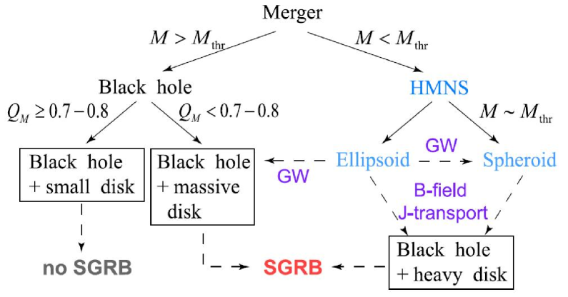
Figure 1.10: Summary about the outcome after the merger. "HMNS", "GW", "B-field" and "J-transport" are hypermassive neutron star, gravitational wave emission, magnetic field, and angular momentum transport, respectively. "Small disk", "massive disk" and "heavy disk" imply that the disk mass is $M_{\rm disk}\ll 0.01M_{\odot}$, $0.01M_{\odot}\leq M_{\rm disk}\leq 0.03M_{\odot}$, and $M_{\rm disk}\geq 0.05M_{\odot}$, respectively (Shibata & Taniguchi 2006).

Besides studies on unmagnetized NS-NS mergers, full GR magneto-hydrodynamics (GRMHD) simulations are indeed necessary to model such NS-NS systems with strong magnetic fields. The first two GRMHD codes capable of evolving the GRMHD equations in dynamical spacetimes were developed by Duez et al. (2005) and Shibata & Sekiguchi (2005). Later they used these codes to study magnetic fields in HMNSs, which are possible transient remnants of binary NS-NS mergers (Duez et al. 2006a, 2006b; Shibata et al. 2006). Secular angular momentum transport due to magnetic braking and the magnetorotational instability results in the collapse of an HMNS to a rotating black hole, accompanied by a gravitational wave burst. The nascent black hole is surrounded by a hot, massive torus undergoing quasistationary accretion and a collimated magnetic field. Recently, Anderson et al. (2008) and Liu et al. (2008) have sued GRMHD codes to study the magnetized NS-NS mergers directly. Anderson et al. (2008) showed that the aligned magnetic fields delay the full merger of the stars compared to the unmagnetized case. Liu et al. (2008) showed that the effects of magnetic fields during and short after the merger phase are significant but not dramatic. The most important role of magnetic fields is long-term, secular evolution of the newly formed disk+BH or HMNS system.

1.4.3 BH-NS Merger Simulations

Mergers of a black hole and a neutron star (BH-NS) is the second class of mergers. Paczyński (1991) and Narayan et al. (1992) also suggested that the merger of a neutron star with a preexisting black hole of several solar masses might produce GRBs. In the dominant formation scenario of binaries consisting of a BH and NS, the BH is formed via hypercritical accretion during a common-envelop phase (Bethe & Brown 1998). The resulting BH has a very low mass ($\sim 3M_{\odot}$) and a NS. Figure 1.11 shows the Newtonian dynamical evolution of a merging BH-NS binary, during which the NS (modeled as a polytrope) is tidally disrupted and an accretion disk promptly forms (Lee & Kluźniak 1999a, 1999b; Lee 2000, 2001).

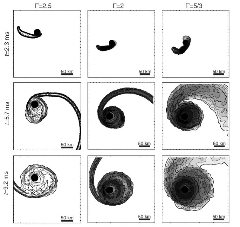
Figure 1.11: The tidal disruption of a NS by a BH in a binary (Lee & Ramirez-Ruiz, 2007) Each column depicts the interaction for a given value of the adiabatic index $\Gamma$ in polytrope EOS. Logarithmic density contours of density (with the lowest one at log (g cm^-3) = 11), are shown in the orbital plane. All three cases initially had identical mass ratios, $Q_{M}=0.31$.

The general conclusion of this body of work, which includes a mock radiation reaction force to account for gravitational wave emission, is that when the orbital separation is of the order of a few stellar radius, the star becomes greatly deformed due to tidal effects, and the system becomes dynamically unstable. for stellar component with relatively stiff EOS ($\Gamma>5/2$), the instability is due to a strong steepening of of the effective potential because of tidal effects mass loss leads to an expansion and Roche lobe overflow, further accelerating the process sand leading to a runaway in which disruption occurs. All of the features anticipated in the work of Lai et al. (1993, 1994) concerning the stability of the binary are apparent, and are also seen in the Rasio & Shapiro (1995). The main additional result in terms of the dynamics is that configurations that are stable in principle up to Roche lobe overflow are de-stabilized by the mass transfer process itself, and fully merge as well within a few orbital periods. It is also clear that in the presence of gravitational radiation reaction, the system enters a dynamical infall at small separations that no amount of mass transfer can revert. Qualitatively, the result is largely independent of the mass ratio, the assumed initial condition in terms of NS spin, both tidally locked and irrotational cases, and the assumed compressibility. Quantitatively, the details are different, and are primarily reflected in the final disk mass and the gravitational waves. Anyway, after a few initial orbital periods, a BH of $M\sim 3-5M_{\odot}$, surrounded by a thick and hot debris disk (torus) with $M_{\rm disk}\sim 0.01-0.1M_{\odot}$ approximately $4\times 10^{7}$cm across is all that remains of the initial couple (Lee & Kluzniak 1999a, 1999b; Lee 2000, 2001; Duez et al. 2002).

It is important to note that the debris disks are formed in only a few dynamical timescale about a few millisecond, which is practically instantaneous considering their later, more leisurely evolution. The possibility that a fraction of the NS in a BH-NS binary would survive the initial mass transfer episode and produce cycles of accretion was explored at long timescales by Davies et al. (2005). This was motivated by the fact that numerical simulations employing relatively stiff equations of state at high binary mass ratios Lee 2000; Rosswog et al. 2004) showed that this might actually occur. However, this is most likely not the case, as the required EOS was unrealistically stiff and gravity was essentially computed in a Newtonian formalism. More recent calculations with pseudo-Newtonian potentials and the use of General Relativity consistently fail to reproduce this behavior for a range of compressibleness in EOS (Rosswog 2005; Lee et al. 2005; Faber et al. 2006a, 2006b). Instead, the neutron star is promptly and fully disrupted soon after the onset of mass transfer.

While Newtonian simulations seen to give a qualitatively correct picture of the dynamics in at least some of the NS-NS mergers scenarios, it is not clear at all that they are applicable also in the case of BH-NS mergers. More importantly, it is also not even clear how to estimate its effects with simple analytical consideration. Computations of the location of the innermost stable circular orbit (ISCO) in black hole systems indicate that tidal disruption may be avoided completely, with the star plunging directly beyond the horizon, essentially being accreted whole in a matter of a millisecond (Miller 2005). This would preclude the formation of a GRB lasting 10 to 100 times longer. But we stress that, just as for stability considerations in the Newtonian case, even if the location of the ISCO can be a useful guide in some cases, it cannot accurately describe the dynamical behavior of the system once mass transfer beings. In pseudo-Newtonian numerical simulation (Rosswog 2005) and post-Newtonian (Prakash et al. 2004), even when a near radial plunge is observed, the star is frequently distorted enough by tidal forces that long tidal tails and disk-like structures can form. The outcome is particularly sensitive to the mass ratio $Q_{M}=N_{\rm NS}/M_{\rm BH}$. Moreover, the spin of the BH is also very important, with rotating BHs favoring the creation of disks. Dynamical calculations of BH-NS systems in pseudo-Newtonian potential that mimic General Relativity effects typically show that for mass ratios $Q_{M}\simeq 0.25$ it is possible to form a disk, although of lower mass than previously thought, $M_{\rm disk}\approx 10^{-2}M_{\odot}$. Faber et al. (2006a, 2006b) presented their results for the dynamical merger phase of a BH-NS binary for low mass ratio ($Q_{M}\simeq 0.1$) using the conformal flatness approximation for GR for a Schwarzschild BH. WHile a polytropic relation with $\Gamma=2$ was assumed, the final outcome is clearly dependent on the complex dynamics of mass transfer. Even though at one point in the evolution most of the stellar material lies within the analytically computed ISCO, tidal torques transfer enough angular momentum to a large fraction of the fluid, producing an accretion disk with $M_{\rm disk}\simeq 0.1M_{\odot}$ by the end of the simulation at $t\simeq 70$ ms. Table 1.8 gives a summary of the disk properties for different progenitors based on the calculations of various groups up to 2006 (Lee & Ramirez-Ruiz 2007).

Prog.	$M_{\rm disk}/M_{\odot}$	Gravity, Method	EOS	References
BH/NS	0.1-0.3	N, SPH	Polytropes	Lee & Kluzniak (1999a, 1999b); Lee 2000, 2001
BH/NS	0.03-0.04	PW, SPH	Polytropes	Lee et al. (2005)
BH/NS	0.26-0.67	N, Grid	LS	Janka et al. (1999)
BH/NS	0.001-0.1	PW, SPH	Shen	Rosswog et al. (2004), Rosswog (2005)
BH/NS	0.001-0.1	GR, SPH	Polytropes	Faber et al. (2006a, 2006b)
NS/NS	0.2-0.5	N, SPH	Polytropes	Rasio & Shapiro (1992, 1994)
NS/NS	0.4	N, SPH	Polytropes	Davies et al. (1994)
NS/NS	0.01-0.25	N, Grid	LS	Ruffert et al. (1996, 1997, 2001)
NS/NS	0.25-0.55	N, SPH	LS	Rosswog et al. (1999, 2000, 2002, 2003), etc.
NS/NS	0.05-0.26	GR, SPH	Shen	Oechislin & Janka (2006)
NS/NS	0.0001-0.01	GR, Grid	APR	Shibata & Taniguchi (2006)

Table 1.8: Remnant disk masses in compact mergers of a variety of equations of state: polytropes, Lattimer & Swesty (LS), Shen et al. (Shen); and various gravity methods: Newtonian (N), Paczynski & WIita (PW), General Relativity (GR). (from Lee & Ramirez-Ruiz , 2007)

Recently, more advanced full relativistic BH-NS simulations were carried out by Shibata & Uryū (2007), Shibata & Taniguchi (2008), Duez et al. (2008), Etienne et al. (2009) and Shibata et al. (2009). Shibata & Taniguchi (2008) studied BH-NS binaries in a quasi-circular orbit as the initial condition and adopted EOS with $\Gamma=2$ and the irrotational velocity fields. They found the resulting torus mass surrounding the BH depends significant on the initial NS mass and radius: $M_{\rm disk}\leq 0.05M_{\odot}$ for $R_{\rm NS}=12$km and $M_{\rm disk}\sim 0.15M_{\odot}$ for $R_{\rm NS}=14.7$km. The total released energy is $\sim 10^{49}$ergs for NS compactness $\leq 0.145$. Etienne et al. (2009) explained the effects of BH spins aligned and antialigned with the orbital angular momentum. Only a small disk $M_{\rm disk}<0.01M_{\odot}$ forms for the antialigned spin core $a/M_{\rm BH}=-0.5$ and for the most extreme-mass -ratio case ($Q_{M}=0.5$). On the other hand, a massive hot disk $M_{disk}\approx 0.7M_{\odot}$ forms in the rapidly spinning aligned ($a/M_{BH}=0.75$). Such a disk could drive a short-hard GRB.

1.4.4 WD-WD Merger Simulations

WD-WD merger scenario (the double-degenerate scenario) has been widely studied as a possible candidate for Type Ia supernova progenitor since Iben & Tutukov (1984) and Webbink (1984). On the other hand, it is not likely that WD-WD mergers could directly lead to GRB phenomena. However, researchers have showed that WD-WD mergers could also form a neutron star remnant in some cases (Saio & Nomoto 1985, 1998; Kawai, Saio & Nomoto 1987; Mochkovitch & Livio 1990; Timmes, Woosley & Taam 1994; Mochkovitch, Guerrero & Segretain 1997; King, Pringle & Wickramasinghe 2001). The newly formed NS, particularly the magnetar or highly magnetized NS, could be the central engine of GRBs (Levan et al. 2006; Chapman et al. 2006). We will discuss the magnetar and neutron star models in §1.5.1.

The process of WD-WD merger itself was first studied by Mochkovitch & Livio (1989, 1990), using an approximate method. The full SPH simulation have been carried out by Benz, Thielemann & Hills (1989), Benz, Cameron & Bowers (1989), Benz, Hill & Thielemann (1989), Benz et al. (1990), Rasio & Shapiro (1995), Segretain et al. (1997), Guerrero et al. (2004); Lorén-Aguilar et al. (2005) Yoon et al. (2007), Shioya et al. (2007) and Lorén-Aguilar et al. (2009). For example, Benz, Hills & Thielemann (1989) studied the mergers of two WDs $0.6+0.6M_{\odot}$ and $0.7+0.9M_{\odot}$ respectively, using 5000 SPH particles. Segretain et al. (1997) used $\sim 6\times 10^{4}$ SPH particles to simulate the coalescence of a $0.9+0.6M_{\odot}$ system. Guerrero et al. (2004) studied a large range of masses and chemical components of the merging binaries, paying special attention to the issue of whether or not thermonuclear runaway occurs during the process of merging. Lorén-Aguilar et al. (2004) studied gravitational wave (GW) radiation from a $0.6+0.6M_{\odot}$ WDs binary, and recently Lorén-Aguilar et al. (2009) adopted a high-resolution SPH code with an improved treatment of the artificial viscosity in this algorithm to study the merging process again. Figure 1.12 shows the temporal evolution of the density for the merger of the $0.6+0.8M_{\odot}$ WD binary system.

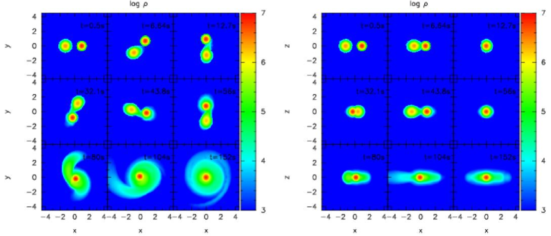
Figure 1.12: Temporal evolution of the density for the coalescence of the $0.6+0.8M_{\odot}$ double WD binary system. The positions of the particles have been projected onto the $xy$ plane (left panels) and in the $xz$ plane (right panels). The disk and central object evolution should be carried out in future study (Lorén-Aguilar et al. 2009).

The first step of WDs binary system evolution in these simulations is more or less the same. The WDs are brought together by GW radiation, until the less massive, and thus the less dense one fils its Roche lobe and begins to transfer mass. However, depending on the initial condition, mass transfer (accretion) could proceed either stably or dynamically unstably, which lead to different outcomes. If the mass transfer process is stable, mass will flow at relatively low accretion rates with a period of order $\sim 10^{6}$ yr. The destruction of the accreting WD in a thermonuclear explosion could produce a Type Ia supernova. On the contrary, unstable accretion make the whole merging process to finish within a few minutes. At such high accretion rate, the primary WD is believed to collapse to form a NS, not to produce a SN Ia. The difference between the two cases relies on the ability of the binary system to return enough angular momentum back to the orbit. In fact, there are two competing processes. On the one hand, the donor star is supported by the pressure of degenerate electrons and, hence, it will expand as it loses mass, thus enhancing the mass-transfer rate. On the other, if orbital angular momentum is conserved the orbit will expand as the donor star loses mass thus reducing the mass-transfer rate. The precise trade-off between both physical processes determines the stability of mass transfer.

Up to this date, almost all the WD-WD merger simulations only adopted SPH code and showed that a compact central object surrounded by a hot corona or disk as the merged configuration. More detailed simulation should be carry out to calculate the evolution of the disk with its angular momentum transfer and the final fate of the central object have been done. And of course, GR or GRMHD methods will instead SPH techniques for the future generation of WD-WD merger simulations.

1.4.5 Gravitational Waves from Merges

Gravitational radiation plays an observable role in the dynamics of many known astronomical systems. Mergers of compact binaries (NS-NS, BH-NS, BH-BH) are expected to be the first cosmological sources of GW detected by ground-based observations. If short-hard GRBs are generated by NS-NS or BH-NS mergers, then they are the electromagnetic counterpart of the most accessible GW sources. In principle the mergers are expected to have three different phases of GW emission: the chirp inspiral signal, the merger signal and the signal from the ringdown of the remaining BH. Figure 1.13 shows an example of GW radiation from Shibata et al. (2009), who studied NS with a polytropic $\Gamma=2$ and the irrotational velocity field tidally disrupted and shallowed by the stellar-mass BH.

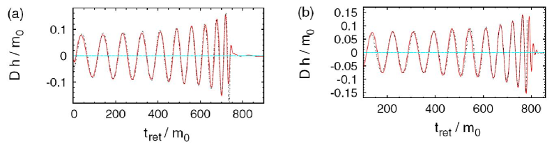
Figure 1.13: Gravitational waveforms observed along the z axis (solid curve) for NS-BH merger models in Shibata et al. (2009). $m_{0}$ is the total mass defined by $M_{\rm BH}$+$M_{\rm NS}$. $h$ denotes a gravitational-wave amplitude and $D$ is a distance between the source and an observer.

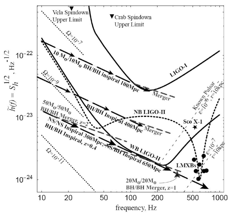
Figure 1.14: The noise $\tilde{h}(f)$ in several planned LIGO interferometers plotted as a function of gravity-wave frequency $f$, and compared with the estimated signal strengths $\tilde{h}_{s}(f)$ from various sources (Cutler & Thorne 2002).

Figure 1.14 shows the three noise curves (LIGO-I, "wide-band" LIGO-II and "narrow-band" LIGO-II), and the possible signal from NS and BH binaries in the last few minutes of their inspiral (Cutler & Thorne 2002). At its current LIGO-I can detect a NS-NS merger up to an average distance of about 15 Mpc, and a merger of a NS with $10M_{\odot}$ BH up to about $30M_{\odot}$. Next generation observatories, such as LIGO-II (advanced-LIGO), are expected to be ten times more sensitive. LIGO-II would detect mergers between NS binary up to $\sim 300$ Mpc, and NS and 10 $M_{\odot}$ BH to 650 Mpc.

1.5 Other Progenitor Models

1.5.1 Magnetized Neutron Star and Magnetar

GRBs were once considered from pulsar-like activities in our Galaxy before 1990s. The "cyclotron features" in the spectra (20-40keV) of several GRBs observed by KONUS and Ginga seemed to support the conclusion that GRBs are produced by strongly magnetized ($\sim 1.7\times 10^{12}$ G) neutron stars with energy releasing rate of $10^{31}$ ergs s^-1 (see §1.1 in detail). Later, however, BATSE and BeppoSAX confirmed that GRBs actually come from cosmological distances, which indicate that most Galactic pulsar models were incorrect. New cosmological pulsar models involving much more energetic pulsar-like activities ($\sim 10^{50}$ ergs s^-1) require the pulsar to be a millisecond-rotation-period NS with very high surface magnetic fields up to $B_{s}>10^{14}$ G.

Neutron star might be formed via the accretion-induced collapse (AIC) of WDs (Nomoto et al. 1979; Canal et al. 1980; Nomoto & Kondo 1991; Usov 1992; Woosley & Baron 1992; Thompson & Duncan 1995; Kluźniak and M. Ruderman 1998; Ruderman et al. 2000; Dessart et al. 2006), the WD-WD binary merges (see §1.4.4) and NS-NS binary mergers (see §1.4.3 and Figure 1.6, or Dai et al. 2006; Gao & Fan 2006) as well as core collapse of massive stars.

AIC of Magnetized WDs to NSs

Some WDs in tight binaries can accrete enough mass from their companions to initiate implosions as they approach the Chandrasekhar limit. After such an implosion begins, there is a competition between energy release from nuclear fusion reactions, which act to explode the star, and the growing rate of electron captures, which removes pressure support and accelerates collapse. The outcome of such WD AIC is Type Ia SNe or NSs. Particularly, NSs could form when the core evolves to sufficiently high density prior to carbon or neon "ignition" (typically $\rho\geq 10^{10}$g cm^-3), that electron captures lead to an underpressure and consequent collapse of the WD (Timmes & Woosley 1992). Figure 1.15 shows the final fate of accreting O+Ne+Mg and C+O WDs, which mainly depends on the mass accretion rate. Also, the outcome for the case WD mass $M\geq 1.1M_{\odot}$ and that of $M\geq 1.1M_{\odot}$ are different. (Nomoto 1986, 1987; Nomoto & Kondo 1991). Next we focus on the case of successful NS formation by WD AIC.

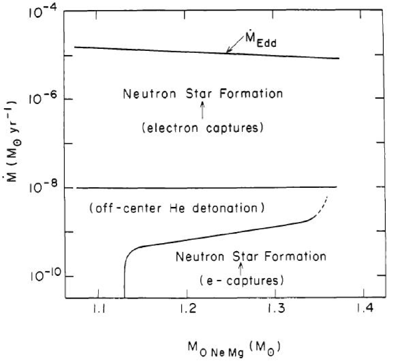
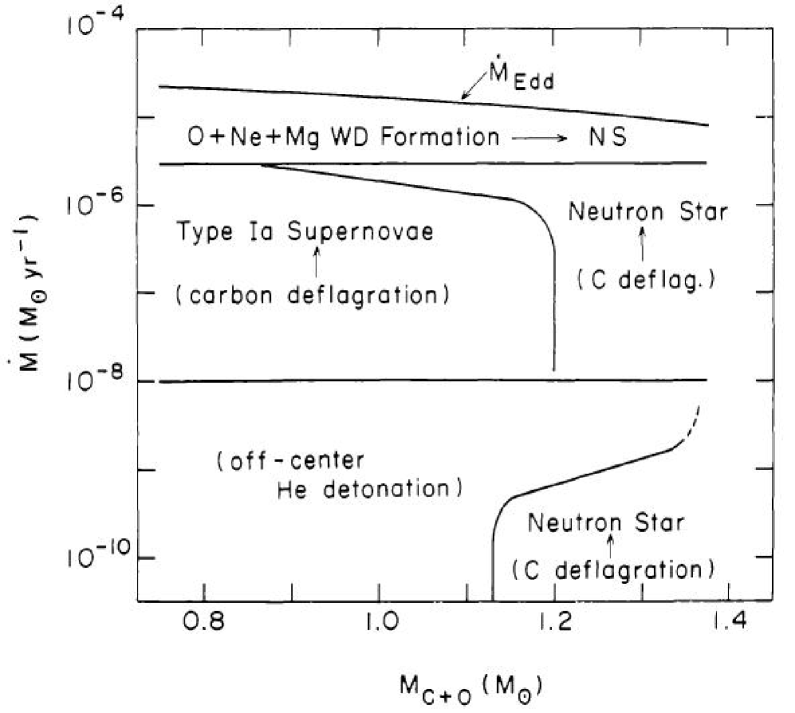
Figure 1.15: The final fate of accreting O+Me+Mg WD (left panel) and C+O WD (right panel) expected for their initial mass and accretion rate $\dot{M}$ (Nomoto & Kondo 1991).

Usov (1992) considered a WD with a surface magnetic fields $B_{s}$ to be a few times of $10^{9}$ G, which might exist, for instance, in magnetic cataclysmic binaries. In the process of collapse, the stellar radius changes from $R_{WD}\approx 10^{9}$ cm for typical WD to $R_{NS}\approx 10^{6}$ cm for Ns, and the surface magnetic fields on the newly formed NS can reach ${B}_{NS}=B_{WD}(R_{WD}/R_{NS})^{2}\sim 10^{15}$ G. Moreover, from angular momentum conservation during the collapse process, the expected angular velocity of the created NS can reach the maximum possible value of NS $\Omega_{NS}\approx 10^{4}$ s^-1 for the angular velocity of WD $\Omega_{WD}\approx 10^{-2}$ s^-1. As a result, the highly magnetized WD could form a millisecond magnetar, which would lose its rotational kinetic energy on a timescale of second or less by electromagnetic or gravitational radiation. Levan et al. (2006) discussed that the WDs with magnetic fields $10^{9}$ G doa actual exist, although they are only in a small fraction $(\sim 10\%$) of all WDs (Figure 1.16). Therefore, it is plausible that the AIC of a WD could create a magnetar, whose magnetic fields are organized mainly by collapse of the WD. Kluźanik & Ruderman (1998) and Ruderman et al. (2000), on the other hand, requires a relatively much lower magnetic fields from WDs $B_{WD}\approx 10^{6}$ G and $B_{NS}\approx 10^{12}$ G for a millisecond-period NS formed by AIC of a WD. The magnetic fields can farther amplified by differential rotating as well as by the AIC process.

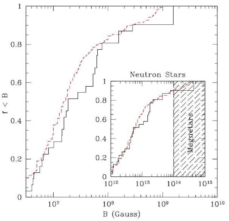
Figure 1.16: The distribution of WD magnetic fields seen in mCVs (black line) and isolated WDs (red dashed) from Levan et al. (2006) and Chapman et al. (2006).

WD-WD and NS-NS Binary Mergers

Strictly speaking, WD-WD merger to form a NS is another process of AIC of a WD. As mentioned in §1.4.4., the less massive star in the WD binary can be tidally disrupted and begin to transfer mass to the primary. A high accretion rate induced by dynamical instability make the accreting primary to become a accretion-induced NS. Levan et al. (2006), Chapman et al. (2006), Chapman, Priddey & Tanvir (2008, 2009) suggested that the scenario of WD-WD merger with a magnetar remnant could be the progenitor of SGRs, and even be the progenitor of a population of nearby short GRBs (Tanvir et al. 2005, Salvaterra et al. 2008), which can be explained as the extra-Galactic SGR giant flares (see also Nakar 2007).

NS-NS merger simulations show that HMNS could be formed in some cases (see §1.4.3 and Figure 1.11). Dai et al. (2006) first suggested that, the new-born magnetic HMNSs, which is formed by NS-NS binary mergers, could be a long-activity GRBs central engine and produce the X-ray flares after the prompt emission (see also Gao & Fan 2006).

Formation of Strong Magnetic Fields in NS

Besides AIC of WDs and compact object mergers, the more commonly way to produce NSs is by core collapse of massive stars, which has been studied for decades since Baade & Zwicky (1934). The problem for GRB progenitors in magnetar mor magnetized NS scenario is that, how could the new-born NS to generate a strong magnetic fields, and extract the rotating energy of NS via magnetic activities to produce a GRB? (Another way to produce a GRB is via thermal hyperaccreting onto the NS, as studied by Zhang & Dai 2008, 2009a and Metzger, Quataert & Thompson 2008. However, the NS with its magnetic fields is still considered the central engine to produce the prompt extension emission or the early afterglow such as X-ray flares.)

The magnetic fields in a magnetar can be as strong as $10^{15}-10^{16}$ G. Such strong fields are generated via three processes: collapse of highly magnetized WDs, amplification from differentially rotation and Paker instability inside the NS, and convective dynamo action during a period of gradient-driven convection after NS formation. Collapse-induced magnetic fields, as mentioned before, satisfied the relation $B_{NS}=B_{WD}(R_{WD}/R_{NS})^{2}$. In this AIC scenario, strong magnetic fields is generated as soon as the NS forms. Differential rotation and convection, on the other hand, could amplify the magnetic fields by extracting the rotating energy to electromagnetic energy for a period of time after NS formation (i.e., post-collapse evolution of magnetic fields). Differential rotation may be caused for two reasons (Thompson & Duncan 1993; Ruderman et al. 2000). First, NSs are less centrally condensed than the degenerate electron pressure-supported cores out of which they form. For a polytropic EOS, the central density $\rho_{c}$ of a WD is $\rho_{c}(WD)\approx 55\bar{\rho}_{WD}$, where $\bar{\rho}_{WD}$ is the initial average WD density. The central density of a NS satisfies $\rho_{c}(NS)\approx 5\bar{\rho}_{NS}$ (Shapiro & Teukolsky 1983). Second, the angular momentum of various mass shells are conserved to a first approximation in the collapse. As a result, the central regions of the newly born NS should initially be spinning much less rapidly than most of the mass in that star by a a factor of about 0.2 (Ruderman et al. 2000).

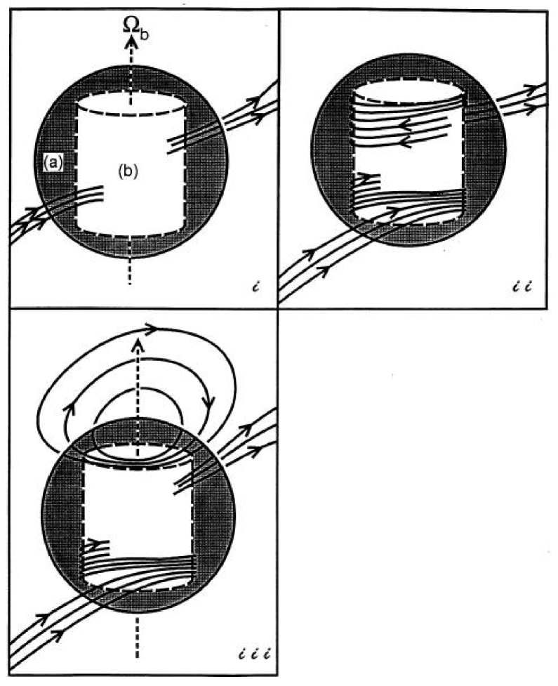
Figure 1.17: Magnetic field evolution in a differential rotation NS for three stages (Kluźanik & Ruderman 1998): (i) poloidal field passing through the NS; (ii) toroidal field amplification; (iii) effect of packer buoyancy instability. See §1.5.1 for detailed discussion.

On the other hand, according to Thompson & Duncan (1993), convection in the NS may be driven by a radial gradient in the lepton number per baryon (Epstein 1979) or by an entropy gradient with the convective velocity $\sim 1.3\times 10^{8}$ cm^-1, after the NS neutrinosphere has shrunk to a radius of $10-20$ km. NS convection is a transient phenomenon and has an extremely high magnetic Reynold number $\sim 10^{17}$. The convective motions are only mildly turbulent on scales larger than the $\sim 10^{2}$ cm neutrino mean free path, but the turbulence is well developed on smaller scales. If the ratio of mean free path, but the turbulence is well developed on smaller scale. If the ratio of mean magnetic pressure to turbulent pressure equals that observed in the upper convection zone of the Sun, and the initial rotation period exceeds $\sim 30$ ms, the energy for field amplification comes mostly from convection, not different rotation, and fields as strong as $3\times 10^{15}$ G can be generated by convection during the first few seconds after NS formation. On the other hand, large-scale $\alpha-\Omega$ dynamo action is possible NS $P\leq 30$ ms to generate strong magnetic fields. For NSs with rapid rotation period $P\sim 1$ ms, the fields generated by differential rotation may be strong enough to suppress convection in some regions, the wrapping of fields around the star by the shear motion allows the formation of large scale magnetic structure. Duncan & Thompson (1992) argued that the fields could reach to $3\times 10^{17}(P/1\textrm{ms})^{-1}$ G as the differential rotation is smoothed by growing magnetic stresses (see also Kluźniak & Ruderman 1998). When the strength of magnetic fields has been sufficiently amplified, the Parker buoyancy tends to change the topology of the fields, drive flux ropes across the surface of the star, where they reconnect, diffuse and eject into the surround medium, and directly provide the energy of GRBs (e.g. Duncan & Thompson 1992; Thompson & Duncan 1993; Kluźanik & Ruderman 1998; Dai & Lu 1998b; Ruderman et al. 2000; Dai et al. 2000).

1.5.2 Supranova Model

Vietri & Stellar (1998, 1999) presented a scenario (they called "supranova model") for the formation of GRBs occuring when a hypermassive neutron star (HMNS) lose so much angular momentum that centrifugal support against self-gravity becomes impossible and the implodes to a BH about 2-3 $M_{\odot}$ surrounded by a transient disk $\sim 0.1M_{\odot}$. The HMNS could be formed directly in the SN explosion of a core with too much mass and angular momentum to end up in a normal NS (Vietri & Stellar 1998), or by accreting matter onto a normal NS from a close companion during a low-mass binary phase (LMXB), while the transport of mass and angular momentum from the secondary makes the NS to become a HMNS (Vietri & Stellar 1999). The maximum mass for a differentially rotating HMNS (Cook, Shapiro & Teukolsky 1994a, 1994b) can reach to $\approx 2-3.5M_{\odot}$. Then the HMNS lose angular momentum via the usual magnetic dipole radiation or gravitational waves radiation. Slowly the HMNS collapses into a BH. Since the neutrinos inside the HMNS have short mean free paths, the implosion from HMNS to BH is almost adiabatic. A mass of $\sim 0.1M_{\odot}$ in the equatorial belt can easily reach centrifugal equilibrium and forms a accretion tours or disk. The new formed BH+disk system is similar to the final results of collapsar and compact object mergers evolution. However, the mechanism of extraction of energy from the system in the supranova scenario is mainly via the conversion of Poynting flux into a magnetized relativistic wind, not the baryonic or neutrino annihilation process.

The advantage of the supranova model is that, it keeps the environment baryon-free. The internal shock scenario requires a small baryon contamination $\sim 10^{-4}M_{\odot}$ to produce a relativistic jet with the bulk Lorentz factor $\Gamma$ to be several hundred (Rees & Mészáros 1992). The powerful wind from a collapsar may still contains lots of baryons, but his is not the case for the supranova model. The GRB jet produced via the collapse of a HMNS does not have to punch a whole through the stellar envelope, both because the former SN explosion has swept away the medium surrounding the remnant, and because of the clean and silent collapse of the HMNS once centrifugal support weakens critically. The small baryon contamination is a natural consequence of the supranova scenario, with typical values of $\sim 10^{-5}M_{\odot}$ well below the $\sim 10^{-4}M_{\odot}$ upper limit.

The main two difficulties of the supranova model are that, the delay between supernova and the following GRB is quite long in this model; and the uncertainty of the torus mass and the lacking of an envelope may not produce long GRBs. Vietri & Stellar (1998) considered the major source of HMNS angular momentum loss is through the usual magnetic dipole radiation. The timescale between a normal SN where a HMNS formed and the implosion to a BH is

$$t_{\rm sd}=\frac{J}{\dot{J}}=10{\rm yr}\frac{j}{0.6}\left(\frac{M}{3M_{\odot}}\right)^{2}\left(\frac{15{\rm km}}{R_{eq}}\right)^{6}\left(\frac{10^{4}{\rm s}^{-1}}{\omega}\right)^{4}\left(\frac{10^{12}{\rm G}}{B}\right)^{2},$$ (1.5)

where the mass in the range of $M\approx 2-3.5M_{\odot}$, equatorial radius $R_{eq}\approx 11-18$ km, angular velocity $\omega\approx 8000-12,000$ s^-1, and the angular momentum $j\approx 0.6-0.78$. However, it is clear in the case of events like GRB 980425 and GRB 030329 that the supernova and the GRB happened nearly simultaneously-within a few days of each other at most (e.g. Hjorth et al. 2003). Therefore, the supranova model, with the long delay betwen SNs and GRBs, could probably only explain few GRB events. Moreover, the main uncertainty in this model is the mass of the formed disk or torus, although Vietri & Stellar estimate a disk $M_{\rm disk}\sim 0.1M_{\odot}$. The mass of the remaining disk depends strongly on the EOS and magnetic fields strength (e.g., Cook, Shapiro & Teukolsky, 1994a, 1994b; Shibata & Shapiro 2002; Shibata 2003; Shapiro 2004; Duez et al. 2006a, 2006b, Stephens et al. 2008). A HMNS with a polytropic and soft EOS $\gamma-4/3\ll 1$, a massive disk may form after its collapse into a BH. On the other hand, Shibata (2003) showed that a HMNS with $\gamma>3/2$ leaves a disk $M_{\rm disk}<10^{-3}M_{\odot}$. However, strong magnetic fields with the MHD angular momentum transfer make a massive disk towards the equator of a HMNS even with a stiff EOS $\Gamma=2$ (Duez et al. 2006a, 2006b; Stephens et al. 2008). Anyway, without an remaining stellar envelope contained around the HMNS, the new formed BH+disk system could only produce short GRBs at most. From this point of view, whether the suprannova scenario allows a lifetime $\geq 1$ Gyr, as mentioned in §1.4, is still questionable.

Chapter 2 Black Hole Accretion Disks, Accretion Flows and GRB Central Engines

Most GRB progenitor scenarios lead to a formation of a stellar-mass black hole and a hyperaccretion disk around it. The accreting black hole system is commonly considered as the direct central engine of GRBs. In this chapter, we first discuss the equations and the classical solutions of the accreting black hole systems, and then focus on the hyperaccreting black-hole disks, which could only be cooled via neutrino emissions.

2.1 Conservation Equations

Basic Equations

The general mass conservation or continuity equation is

$$\frac{\partial\rho}{\partial t}+\nabla\cdot(\rho\textbf{v})=0.$$ (2.1)

Moreover, the general momentum conservation equation with viscosity, i.e., the Navier-Stokes equation is (Landau & Lifshitz, 1959)

$$\frac{\partial\textbf{v}}{\partial t}+(\textbf{v}\cdot\nabla)\textbf{v}=-\frac{1}{\rho}\nabla p-\nabla\Phi+\frac{\eta}{\rho}\triangle\textbf{v}+(\xi+\frac{\eta}{3})\nabla(\nabla\cdot\textbf{v}),$$ (2.2)

where $\Phi$ is the gravitational potential, the constant $\eta$ and $\xi$ are called coefficients of viscosity. For incompressible fluid, the term $(\xi+\eta/3)\nabla(\nabla\cdot\textbf{v})$ in the right hand of equation 2.2 is vanished.

For accretion disks under axial symmetry assumption, we adopt cylindrical coordinates ($r,\varphi,z$), and take $\partial/\partial\varphi=0$. Three velocity components of accretion flow at a radius $r$ from the central compact object ($v_{r},v_{\varphi},v_{z}$) can be divided into two parts: an toroidal component $v_{\phi}=\Omega r$ with $\Omega$ as the disk angular velocity, and a small poloidal component $\textbf{v}_{p}=(v_{r},v_{z})$. If we also consider the disk is in a steady state, i.e., $\partial/\partial t=0$. Then the mass conservation equation can be written as

$$\frac{1}{r}\frac{\partial}{\partial r}(\rho rv_{r})+\frac{\partial}{\partial z}(\rho v_{z})=0.$$ (2.3)

The three components of the momentum equation are (Frank, King & Raine 2002)

$$v_{r}\frac{\partial v_{r}}{\partial r}+v_{z}\frac{\partial v_{r}}{\partial z}=(\Omega^{2}-\Omega_{K}^{2})r-\frac{1}{\rho}\frac{\partial p}{\partial r}+\frac{1}{\rho}\left[\frac{\partial\sigma_{rr}}{\partial r}+\frac{\sigma_{rr}-\sigma_{\varphi\varphi}}{r}+\frac{\partial\sigma rz}{\partial z}\right],$$ (2.4)

$$v_{r}\frac{\partial v_{z}}{\partial r}+v_{z}\frac{\partial v_{z}}{\partial z}=-\Omega_{K}^{2}z-\frac{1}{\rho}\frac{\partial p}{\partial z}+\frac{1}{\rho}\left[\frac{1}{r}\frac{\partial(r\sigma_{rz})}{\partial r}+\frac{\partial\sigma_{zz}}{\partial z}\right],$$ (2.5)

$$\frac{v_{r}}{r}\frac{\partial(r^{2}\Omega)}{\partial r}+v_{z}\frac{\partial(r\Omega)}{\partial z}=\frac{1}{\rho}\left[\frac{1}{r^{2}}\frac{\partial(r^{2}\sigma_{r\varphi})}{\partial r}+\frac{\partial\sigma_{\varphi z}}{\partial z}\right],$$ (2.6)

where $\Omega_{K}$ is the Kepler angular velocity $\Omega_{K}=\sqrt{(GM)/r^{3}}$ with $M$ being the mass of central star, and the nine components of stress tensor $\sigma$ for incompressible fluid are

$$\sigma_{r\varphi}=\sigma_{\varphi r}=\mu r\frac{\partial\Omega}{\partial r},$$

$$\sigma_{rz}=\sigma_{zr}=\mu\left(\frac{\partial v_{z}}{\partial r}+\frac{\partial v_{r}}{\partial z}\right),$$

$$\sigma_{\varphi z}=\sigma_{z\varphi}=\mu\frac{\partial(r\Omega)}{\partial z},$$

$$\sigma_{rr}=2\mu\frac{\partial v_{r}}{\partial r},\sigma_{zz}=2\mu\frac{\partial v_{z}}{\partial z},\sigma_{\varphi\varphi}=2\mu\frac{v_{r}}{r}.$$ (2.7)

The axial symmetry assumption and the disk geometry half-height $H\ll$ radius $r$ allows us to take the approximation that the terms $v_{z}$ and $\partial/\partial z$ are much smaller compared to other terms in equations (2.4) to (2.6). The the radial component of the momentum equation (2.4) can be simplified as

$$v_{r}\frac{\partial v_{r}}{\partial r}=(\Omega^{2}-\Omega_{K}^{2})r-\frac{1}{\rho}\frac{\partial p}{\partial r}+\frac{2}{\rho r}\left[\frac{\partial}{\partial}\left(\mu\frac{\partial v_{r}}{\partial r}\right)+\mu\frac{\partial}{\partial r}\left(\frac{v_{r}}{r}\right)\right].$$ (2.8)

The angular momentum equation (2.6) to be

$$\frac{v_{r}}{r}\frac{\partial(r^{2}\Omega)}{\partial r}=\frac{1}{\rho r^{2}}\frac{\partial}{\partial r}\left(\mu r^{3}\frac{\partial\Omega}{\partial r}\right).$$ (2.9)

The z-direction momentum equation (2.5) be rewritten as

$$\Omega_{K}^{2}z+\frac{1}{\rho}\frac{\partial p}{\partial z}\approx 0.$$ (2.10)

For ’thin’ disk with $z\ll H$, we can set $|\partial p/\partial z|\sim p/H$ and $z\sim H$, the half-height of the disk $H$ satisfies

$$H\cong\frac{c_{s}}{\Omega_{K}}.$$ (2.11)

where $c_{s}=\sqrt{p/\rho}$ is the isothermal sound speed. Furthermore, the energy balance in a steady-state disk is established among the heating rate $q^{+}$, the cooling rate $q^{-}$ and the advection rate $q_{\rm adv}$ per unit volume. The heating rate term $q^{+}$ is usually contributed by local viscous dissipation (Thompson 1972)

$$q^{+}=\mu r^{2}\left(\frac{d\Omega}{dr}\right)^{2}.$$ (2.12)

Cooling is mainly via phonon or high-energy particle emissions. The advection term $q_{\rm adv}$ is energy flux driven by entropy gradient in the accretion process. Thus the local energy conservation energy is written

$$q_{\rm adv}=\rho v_{r}T\frac{ds}{dr}=q^{+}-q^{-}.$$ (2.13)

where $s$ is the specify entropy and $T$ is the temperature of the disk at radius $r$.

Conversation equations (2.3), (2.8), (2.9), (2.13) and relation (2.11) are commonly used for disks under the assumptions of axisymmetry and ’thin’ disk geometry (e.g., Abramowicz et al. 1988; Narayan & Popham 1993; Narayan & Yi 1994).

$\alpha$-Prescription

The radio of dynamic viscosity $\eta$ and the density $\rho$ ,i. e., $\nu=\eta/\rho$, is called the kinematic viscosity. We adopt the relation that the kinematic viscosity $\nu$ is proportional to the isothermal sound speed $c_{s}$ and the disk half-thickness $H$, and write

$$\nu=\alpha c_{s}H.$$ (2.14)

with the viscosity parameter $\alpha\leq 1$ in most cases. This famous $\alpha$-prescription was first adopted by Shakura & Sunyave (1973) from another point of view. More detailed description based on microphysics scenario can be seen in many classical references (e.g., Landau & Lifshitz 1959; Frank et al. 2002). Although MHD simulations beyond $\alpha$-prescription for understanding the physical mechanisms which may generate a viscosity in disks have been carried out for years (see Balbus & Hawley 1998 for a review), the $\alpha$-prescription, which is a much simpler treatment with clear physical scenario, is still very useful and will continue to be used for analytic and semi-analytic calculations. Now we use the relation $\mu=\nu\rho=\alpha c_{s}\rho H$ in all of our equations.

Vertically Integrated Equations

A farther reasonable approximation treatment which could simplify the group of partial differential equations and make them to be differential equations, is the "vertical integration" treatment along the $z$-direction. The disk may be described by vertically average physical quantities as a function of radius $r$. The surface density is $\sum=2\rho H$. Thus the equations of continuity, radial and angular momentum (2.3, 2.8, 2.9) are

$$\dot{M}=-2\pi rv_{r}\Sigma,$$ (2.15)

$$v_{r}\frac{dv_{r}}{dr}=(\Omega^{2}-\Omega_{K}^{2})r-\frac{1}{\sum}\frac{d}{dr}\left(\Sigma c_{s}^{2}\right),$$ (2.16)

$$\frac{v_{r}}{r}\frac{d(r^{2}\Omega)}{dr}=\frac{1}{\Sigma r^{2}}\frac{d}{dr}\left(\Sigma\nu r^{3}\frac{d\Omega}{dr}\right),$$ (2.17)

The angular equation (2.17) can be further integrated. If we take the angular velocity of the accretion flow $\Omega\approx\Omega_{K}$, then we obtain the angular momentum equation as

$$\nu\Sigma=\frac{\dot{M}}{3\pi}f,$$ (2.18)

where $f=1-l_{0}/l$ with $l=r^{2}\Omega$ is the specific angular momentum and $l_{0}$ is the special angular momentum constant at the inner edge of the disk. Usually we can write $f=1-\sqrt{r_{*}/r}$ with $r_{*}$ being the inner edge of the disk (Frank et al. 2002). Furthermore, combining equations (2.12) and (2.18) the vertically intergraded local viscous dissipation rate of a nearly Keplerian disk is

$$Q^{+}=\frac{3}{8\pi}\frac{GM\dot{M}}{r^{3}}f,$$ (2.19)

and the integrated energy equation is

$$\frac{1}{2}\Sigma Tv_{r}\frac{ds}{dr}=\frac{3}{8}\frac{GM\dot{M}}{8\pi r^{3}}f-Q^{-}.$$ (2.20)

The factor 1/2 in the left side of equation (2.20) is added because we only study the vertically-integrated energy equation over a half-thickness $H$.

2.2 Equations for Magnetized Flows

For magnetized accretion flows, we need to consider the effects of magnetic fields on momentum transfer and energy dissipation. The momentum equation of accretion flows (2.2) is modified as

$$\frac{\partial\textbf{v}}{\partial t}+(\textbf{v}\cdot\nabla)\textbf{v}=-\frac{1}{\rho}\nabla p-\nabla\Phi+\frac{\eta}{\rho}\triangle\textbf{v}+\frac{1}{\rho c}\textbf{J}\times\textbf{B},$$ (2.21)

with the added term of Lorentz force in the right side of the equation. The current density $J$ satisfies

$$\textbf{J}=\frac{4\pi}{c}(\nabla\times\textbf{B}),$$ (2.22)

In cylindrical coordinates ($r,\varphi,z$), the three components of Lorentz force are

$$\frac{1}{\rho c}(\textbf{J}\times\textbf{B})_{r}=-\frac{1}{2\rho}\frac{\partial}{\partial r}\left(\frac{B_{\varphi}^{2}+B_{z}^{2}}{4\pi}\right)+\frac{B_{z}}{4\pi\rho}\frac{\partial B_{z}}{\partial z}-\frac{B_{\varphi}^{2}}{4\pi\rho r},$$ (2.23)

$$\frac{1}{\rho c}(\textbf{J}\times\textbf{B})_{\varphi}=\frac{B_{r}B_{\varphi}}{4\pi\rho}+\frac{B_{r}}{4\pi\rho}\frac{\partial B_{\varphi}}{\partial r}+\frac{B_{z}}{4\pi\rho}\frac{\partial B_{\varphi}}{\partial z},$$ (2.24)

$$\frac{1}{\rho c}(\textbf{J}\times\textbf{B})_{r}=-\frac{1}{2\rho}\frac{\partial}{\partial z}\left(\frac{B_{\varphi}^{2}+B_{z}^{2}}{4\pi}\right)+\frac{B_{r}}{4\pi\rho}\frac{\partial B_{z}}{\partial r}.$$ (2.25)

The right side of equations (2.23), (2.23) and (2.23) need to be added to the right side of equations (2.4), (2.5) and (2.6) respectively.

The energy equation should include Joule dissipation (or Ohmic dissipation) as well as viscous dissipation,

$$\rho v_{r}T\frac{ds}{dr}=q^{+}_{\rm vis}+q^{+}_{\rm Joule}-q^{-},$$ (2.26)

where

$$q^{+}_{\rm Joule}=\frac{4\pi}{c^{2}}\eta_{m}\textbf{J}^{2}$$

$$=\frac{\eta_{m}}{4\pi}\left(\frac{\partial B_{\varphi}}{\partial z}\right)^{2}+\frac{\eta_{m}}{4\pi}\left(\frac{\partial B_{r}}{\partial z}-\frac{\partial B_{z}}{\partial r}\right)^{2}+\frac{\eta_{m}}{4\pi r^{2}}\left[\frac{\partial}{\partial r}(rB_{\varphi})\right]^{2}$$ (2.27)

with $\eta_{m}$ being the magnetic diffusivity of the disk. If we define the Alfvén sound speeds along the three directions $c_{r,\varphi,z}^{2}=B_{r,\varphi,z}^{2}/(4\pi\rho)$, then the vertically integrated momentum equations read (Zhang & Dai 2008b)

$$v_{r}\frac{\partial v_{r}}{\partial r} = (\Omega^{2}-\Omega_{K}^{2})r-\frac{1}{\Sigma}\frac{\partial}{\partial r}(\Sigma c_{s}^{2})$$ (2.28)

$$-\frac{1}{2\Sigma}\frac{\partial}{\partial r}[\Sigma(c_{z}^{2}+c_{\varphi}^{2})]+\frac{1}{\sqrt{\Sigma}}c_{z}\frac{\partial}{\partial z}(\sqrt{\Sigma}c_{r})-\frac{c_{\varphi}^{2}}{r},$$

$$\frac{v_{r}}{r}\frac{\partial(rv_{\varphi})}{\partial r}+v_{z}\frac{\partial v_{\varphi}}{\partial z} = \frac{1}{\Sigma r^{2}}\frac{\partial}{\partial r}\left(\Sigma\nu r^{3}\frac{\partial\Omega}{\partial r}\right)$$ (2.29)

$$+\frac{c_{r}c_{\varphi}}{r}+\frac{c_{r}}{\sqrt{\Sigma}}\frac{\partial}{\partial r}(\sqrt{\Sigma}c_{\varphi})+\frac{c_{z}}{\sqrt{\Sigma}}\frac{\partial}{\partial z}(\sqrt{\Sigma}c_{\varphi}),$$

$$\frac{v_{r}}{r}\frac{\partial v_{z}}{\partial r} = -\Omega_{K}^{2}z-\frac{1}{\Sigma}\frac{\partial}{\partial z}(\Sigma c_{s}^{2})$$ (2.30)

$$-\frac{1}{2\Sigma}\frac{\partial}{\partial z}[\Sigma(c_{r}^{2}+c_{\varphi}^{2})]+\frac{1}{\sqrt{\Sigma}}c_{r}\frac{\partial}{\partial r}(\sqrt{\Sigma}c_{z}).$$

And the energy conservation equation becomes

$$\frac{1}{2}\Sigma v_{r}T\frac{ds}{dr} = \frac{3}{8\pi}\frac{GM\dot{M}}{r^{3}}f+\eta_{m}\left[\frac{\partial}{\partial z}\left(\sqrt{\Sigma}c_{\varphi}\right)\right]^{2}$$ (2.31)

$$\eta_{m}\left[\frac{\partial}{\partial z}\left(\sqrt{\Sigma}c_{r}\right)-\frac{\partial}{\partial r}\left(\sqrt{\Sigma}c_{\varphi}\right)\right]^{2}+\frac{\eta_{m}}{r^{2}}\left[\frac{\partial}{\partial r}(r\sqrt{\Sigma}c_{\varphi})\right]^{2}.$$

Lovelace, Wang & Sulkanen (1987) derived similar momentum equations as (2.28) to (2.31). The magnetic fields symmetry requires

$$B_{r}(r,z)=+B_{r}(r,-z),$$

$$B_{\varphi}(r,z)=+B_{\varphi}(r,-z),$$

$$B_{z}(r,z)=-B_{z}(r,-z)..$$ (2.32)

The $r,\varphi,z$-component equations are

$$\Sigma v_{r}\frac{\partial v_{r}}{\partial r}=\Sigma\frac{v_{\varphi}^{2}}{r}-\Sigma\frac{GM}{r^{2}}-\frac{1}{8\pi r^{2}}\frac{\partial}{\partial r}[2Hr^{2}<(B_{\varphi}^{2}-B_{r}^{2})>]+\frac{1}{4\pi}B_{r}B_{z}|_{z=-H}^{z=H},$$ (2.33)

$$\frac{\dot{M}}{3\pi}f=\Sigma\nu+\frac{1}{3\pi\Omega}\left[\left(\frac{r_{*}}{r}\right)^{2}<B_{r}B_{\varphi}>_{r=r_{*}}-<B_{r}B_{\varphi}>\right],$$ (2.34)

$$\left(\frac{GM\Sigma}{2r^{3}}\right)\left(\int_{0}^{H}z\rho dz/\int_{0}^{H}\rho dz\right)=p|_{z=0}-\frac{B_{r}^{2}+B_{\varphi}^{2}}{8\pi},$$ (2.35)

respectively, where $<...>$ is defined as

$$<B_{\xi}>=\frac{1}{2H}\int_{-H}^{H}dzB_{\xi}(r,z).$$ (2.36)

2.3 Photon Radiation and Shakura-Sunyaev Solutions

In accretion disks, the vertical energy transfer mechanism may be either radiative or convective, depending on the temperature gradient along the $z$-direction. We will discuss the convection effect later in §1.1.4. In this section we first consider the energy transfer is radiative. The specific flux is

$$F_{\nu}(z)=-\frac{4\pi}{3\kappa_{\nu}\rho}\frac{\partial B_{\nu}(T)}{\partial z},$$ (2.37)

where $\kappa_{\nu}$ is the opacity coefficient for a particular frequency $\nu$. Here we assume the radiation field in the disk has reached thermal equilibrium in the layer $z$ to $z+dz$, and $B_{\nu}(T)$ is the Planck blackbody function. Intergrading (2.37) over frequency we obtain

$$F(z)=\int_{0}^{\infty}F_{\nu}(z)dz=-\frac{c}{3\kappa_{R}\rho}\frac{\partial}{\partial z}(a_{B}T^{4})=-\frac{4c\sigma_{B}}{3\kappa_{R}\rho}\frac{\partial}{\partial z}(T^{4}),$$ (2.38)

where $a_{B}$ is the radiation constant while $\sigma_{B}$ the Stefan-Boltzmann constant, $\kappa_{R}$ is the Rosseland mean opacity. Hubeny (1990, see also Popham & Narayan 1995) derived an more elaborate expression for the vertical flux

$$F(z)=\frac{\sigma_{B}T^{4}}{3(\tau/2+1/\sqrt{3}+1/3\tau_{a})},$$ (2.39)

where $\tau=\kappa_{R}\rho H$ and $\tau_{a}=\kappa_{a}\rho H$ are the total and absorption optical depths.

The generated dissipation energy in the disk is mainly cooled by thermal photon emission. Thus we have the cooling rate $Q^{-}_{\rm rad}$ over a half-thickness disk

$$Q^{-}_{\rm rad}=\int_{0}^{H}\frac{\partial F(z)}{\partial z}dz=F(H)-F(0).$$ (2.40)

We adopt the simplified energy equation, i.e., energy balance is established between radiation and viscous dissipation

$$Q^{-}_{\rm rad} =F(H)-F(0)=\frac{4\sigma_{B}T_{c}^{4}}{3\tau}$$ (2.41)

$$=\int_{0}^{H}q^{+}_{\rm vis}(z)=Q^{+}_{\rm vis}=\frac{3}{8\pi}\frac{GM\dot{M}}{r^{3}}f.$$

$T_{c}$ is the central temperature at $z$=0, and we assume $T_{c}\gg T(H)$. The main contribution to the opacity for a normal thermal disk comes from Thompson scattering on free electrons, and free-free absorption (Shakura & Sunyave 1973)

$$\sigma_{T}=6.65\times 10^{-25}\textrm{cm}^{2},\sigma_{ff}=0.11T^{-7/2}n\textrm{cm}^{3}\textrm{g}^{-1},$$ (2.42)

For a complete set of equations we also need thermodynamical equation, or the expression of pressure, which include both gas pressure and radiation pressure

$$p=p_{g}+p_{r}=\frac{\rho T\Re}{\mu_{\rm acc}}+\frac{4\sigma_{B}}{3c}T_{c}^{4},$$ (2.43)

where $\Re$ is the gas constant, $\mu_{\rm acc}$ is the mean molecular weight.

Combining equations (2.11), (2.14), (2.18), (2.41), (2.42) and (2.43), we are able to determine the physical properties of a thin photon radiative disk as functions of accretion rate $\dot{M}$, central object mass $M$, radius $r$ and inner edge radius $r_{*}$. The analytical solutions were first derived by Shakura & Sunyaev (1973), who divided the disk into three regions, and gave different solution in different region:

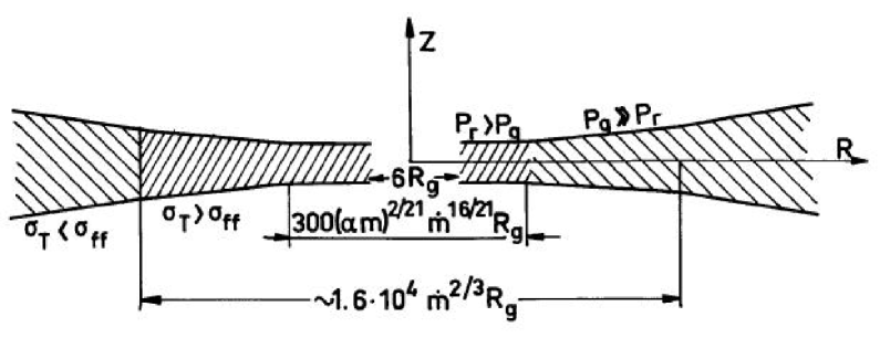
Figure 2.1: Physical scenario of Shakura & Sunyavae disk.

a) $p_{r}\gg p_{g}$, $\sigma_{T}\gg\sigma_{ff}$

$$\Sigma=4.6\alpha^{-1}m^{-1}\hat{r}^{3/2}f^{-1}$$

$$T=2.3\times 10^{7}(\alpha m)^{-1/4}\hat{r}^{-3/4}$$

$$n=\Sigma/(2Hm_{p})=4.3\times 10^{17}\alpha^{-1}\dot{m}^{-2}m^{-1}\hat{r}^{3/2}f^{-2}$$

$$H=3.2\times 10^{6}\dot{m}mf$$

$$v_{r}=7.7\times 10^{7}\alpha\dot{m}^{2}\hat{r}^{-5/2}f,$$ (2.44)

b) $p_{g}\gg p_{r}$, $\sigma_{T}\gg\sigma_{ff}$

$$\Sigma=1.7\times 10^{5}\alpha^{-4/5}\dot{m}^{3/5}m^{1/5}\hat{r}^{-3/5}f^{3/5}$$

$$T=3.1\times 10^{8}\alpha^{-1/5}\dot{m}^{2/5}m^{-1/5}\hat{r}^{-9/10}f^{2/5}$$

$$n=4.2\times 10^{24}\alpha^{-7/10}\dot{m}^{2/5}m^{-7/10}\hat{r}^{-33/20}f^{2/5}$$

$$H=1.2\times 10^{4}\alpha^{-1/10}\dot{m}^{1/5}m^{9/10}r^{21/20}f^{1/5}$$

$$v_{r}=2\times 10^{6}\alpha^{4/5}\dot{m}^{2/5}m^{-1/5}\hat{r}^{-2/5}f^{-3/5},$$ (2.45)

b) $p_{g}\gg p_{r}$, $\sigma_{ff}\gg\sigma_{T}$

$$\Sigma=6.1\times 10^{5}\alpha^{-4/5}\dot{m}^{7/10}m^{1/5}\hat{r}^{-3/4}f^{7/10}$$

$$T=8.6\times 10^{7}\alpha^{-1/5}\dot{m}^{3/10}m^{-1/5}\hat{r}^{-3/4}f^{3/10}$$

$$n=3\times 10^{25}\alpha^{-7/10}\dot{m}^{11/20}m^{-7/10}\hat{r}^{-15/8}f^{11/20}$$

$$H=6.1\times 10^{3}\alpha^{-1/10}\dot{m}^{3/20}m^{9/10}\hat{r}^{9/8}f^{3/20}$$

$$v_{r}=5.8\times 10^{5}\alpha^{4/5}\dot{m}^{3/10}m^{-1/5}\hat{r}^{-1/4}f^{-7/10},$$ (2.46)

where

$$m=\frac{M}{M_{\odot}},\dot{m}=\frac{\dot{M}}{\dot{M}_{cr}}=\frac{\dot{M}}{3\times 10^{-8}M_{\odot}yr^{-1}}\times\left(\frac{M_{\odot}}{M}\right),\hat{r}=\frac{r}{3r_{g}}=\frac{1}{m}\left(\frac{r}{9\textrm{km}}\right),$$ (2.47)

and the units of surface density $\Sigma$, temperature $T$, number density $n$, half-thickness $H$ and radial velocity $v_{r}$ are g cm^-2, K, cm^-3, cm and cm s^-1. The general scenario of the disk structure is summarized in Figure 2.1, which shows the three regions having different physical properties.

2.4 Accretion Flows with Self-Similar Structure

We switch back to the basic energy equation (2.13)

$$q_{\rm adv}=q^{+}-q^{-}$$

where $q_{\rm adv}$ is the advection transport of energy driven by the entropy gradient. In last section §2.1.3, we approximately set $q_{\rm adv}\simeq 0$. In fact, depending on the relative magnitudes of the terms in equation (2.13), we may identify three cases of accretion flows (Narayan, Mahadevan & Quataert, 1998)

• $q^{+}\simeq qq^{-}\gg q_{\rm adv}$, the cooling-dominated flow where all the energy released by viscous stresses is radiated. The S-S thin disk solutions correspond to this case.

• $q_{\rm adv}\simeq q^{+}\gg qq^{-}$, an advection-dominated accretion flow (ADAF) where almost all the viscous energy is stored in the gas and is deposited into the central BH. For a given $\dot{M}$, an ADAF is much less luminous than a cooling-dominated flow. Moreover, the effect of convection in an ADAF is significant for sufficiently low viscosity parameter $\alpha$. Convective ADAF is called "convection-dominated accretion flow" (CDAF, Narayan et al. 2000).

• $-q_{\rm adv}\simeq q^{-}\gg qq^{+}$, advection-cooling-balance accretion flow, where energy generation by viscosity is negligible, but the entropy of the inflowing gas is converted to radiation.

Self-similar treatment is very useful to describe the properties of various fluid since Sedov (1969) and Taylor (1950). The analytical ADAF solution based on self-similar treatment has been derived by Narayan & Yi (1994). The integrated equations (2.15), (2.16), (2.17) and the energy equation

$$\Sigma v_{r}T\frac{ds}{dr}=\frac{3+3\epsilon}{2}\Sigma\nu\frac{dc_{s}^{2}}{dr}-2c_{s}^{2}Hv_{r}\frac{d\rho}{dr}=f\frac{\alpha\Sigma c_{s}^{2}r^{2}}{\Omega_{K}}\left(\frac{d\Omega}{dr}\right)^{2}$$ (2.48)

permit a self-similar solution of the form (Spruit et al. 1987):

$$\rho\propto r^{-3/2},v_{r}\propto r^{-1/2},\Omega\propto r^{-3/2},c_{s}^{2}\propto r^{-1}$$ (2.49)

Here $\epsilon=p_{r}/p$ is the fraction of radiation pressure, and $f$ measures the degree to which the flow is advection-dominated. Thus the self-similar solution of an ADAF is (Narayan & Yi, 1994)

$$v_{r}(r)=-(5+2\epsilon^{\prime})\frac{g(\alpha,\epsilon^{\prime})}{3\alpha}v_{K}$$ (2.50)

$$\Omega(r)=\left[\frac{2\epsilon^{\prime}(5+2\epsilon^{\prime})g(\alpha,\epsilon^{\prime})}{9\alpha^{2}}\right]^{1/2}\Omega_{K}$$ (2.51)

$$c_{s}^{2}(r)=\frac{2(5+2\epsilon^{\prime})}{9}\frac{g(\alpha,\epsilon^{\prime})}{\alpha^{2}}v_{K}^{2}$$ (2.52)

where

$$v_{K}\equiv\left(\frac{GM}{r}\right)^{1/2},\epsilon^{\prime}\equiv\frac{\epsilon}{f}=\frac{1}{f}\left(\frac{5/3-\gamma}{\gamma-1}\right),g(\alpha,\epsilon^{\prime})\equiv\left[1+\frac{18\alpha^{2}}{(5+2\epsilon^{\prime})}\right]^{1/2}-1$$ (2.53)

Taking the assumption $\alpha^{2}\ll 1$, the solution (2.50) to (2.52) takes a simple form

$$\frac{v}{v_{K}}\approx-\frac{3\alpha}{5+2\epsilon^{\prime}},\frac{\Omega}{\Omega_{K}}\approx\left(\frac{2\epsilon^{\prime}}{5+2\epsilon^{\prime}}\right)^{1/2},\left(\frac{c_{s}}{v_{K}}\right)^{2}\approx\frac{2}{5+2\epsilon^{\prime}}$$ (2.54)

In the limit of very efficient cooling, $f\rightarrow 0$ and $\epsilon^{\prime}\rightarrow 0$, we obtain $v_{r},c_{s}\ll v_{K}$ and $\Omega\rightarrow\Omega_{K}$, which correspond the Keplerian accretion flows. In the opposite limit of an ADAF $f\rightarrow 1$, we have the extreme case $\Omega\rightarrow 0$ for $\gamma\rightarrow 5/3$ and $c_{s}\sim v_{K}$, $H\sim c_{s}/v_{K}\sim v_{K}/\Omega_{K}=r$, which correspond to the spherical Bondi accretion limit.

Next we discuss the effect of convection in ADAFs. The $r$-direction integrated form of angular momentum equation (2.9) read

$$0=\dot{J}_{v}+\dot{J}_{\rm adv}=-\alpha\frac{c_{s}^{2}}{\Omega_{K}}\rho r^{3}\frac{d\Omega}{dr}+\rho rv_{r}\Omega r^{2},$$ (2.55)

where the viscosity next flux

$$\dot{J}_{v}=-\alpha\frac{c_{s^{2}}}{\Omega_{K}}\rho r^{3}\frac{d\Omega}{dr}.$$ (2.56)

Analogous to the viscosity flux and viscosity parameter $\alpha$, Narayan et al. (2000) introduced the "convection parameter" $\alpha_{c}$ and the angular flux due to convection as

$$\dot{J}_{c}=-\alpha_{c}\frac{c_{s}^{2}}{\Omega_{K}}\rho r^{3(1+g)/2}\frac{d}{dr}[\Omega r^{3(1-g)/2}],$$ (2.57)

with the index $g$ describes the physics of convective angular momentum transport. When $g=1$, expression (2.57) becomes

$$\dot{J}_{c}=-\alpha_{c}\frac{c_{s}^{2}}{\Omega_{K}}\rho r^{3}\frac{d\Omega}{dr},$$ (2.58)

convection angular momentum flux is oriented down the angular velocity gradient. While when $g=-1/3$,

$$\dot{J}_{c}=-\alpha_{c}\frac{c_{s}^{2}}{\Omega_{K}}\rho r\frac{d\Omega r^{2}}{dr},$$ (2.59)

convection angular momentum flux is due to the specific angular momentum gradient. The $r$-direction angular momentum equation reads

$$0=\dot{J}_{v}+\dot{J}_{c}+\dot{J}_{\rm adv}=-\alpha\frac{c_{s}^{2}}{\Omega_{K}}\rho r^{3}\frac{d\Omega}{dr}-\alpha_{c}\frac{c_{s}^{2}}{\Omega_{K}}\rho r^{3(1+g)/2}\frac{d}{dr}[\Omega r^{3(1-g)/2}]+\rho rv_{r}\Omega r^{2}.$$ (2.60)

We take the diffusion constant $K_{c}$ as

$$K_{c}=\alpha_{c}\frac{c_{s}^{2}}{\Omega_{K}},$$ (2.61)

and the energy flux via convection is

$$F_{c}=-K_{c}\rho\frac{de}{dt}=-\alpha_{c}\frac{c_{s}^{2}}{\Omega_{K}}\rho T\frac{ds}{dr}.$$ (2.62)

Thus the energy transport by convection in cylindrical coordinates is $r^{-1}d(rF_{c})/dr$. In this section we follow Narayan et al. (2000) and adopt the expression $r^{-2}d(r^{2}F_{c})/dr$ in spherical coordinates and obtain the energy equation including convection as

$$\rho v_{r}T\frac{ds}{dr}+\frac{1}{r^{2}}\frac{d}{dr}(r^{2}F_{c})=Q^{+}=(\alpha+\alpha_{c})\frac{c_{s}^{2}}{\Omega_{K}}\rho r^{2}\left(\frac{d\Omega}{dr}\right)^{2}.$$ (2.63)

The radial momentum equation (2.8), and new angular momentum and energy equations (2.60) and (2.62) allow us to obtain the self-similar solutions for ADAF with convection. We take the self-similar structure

$$\rho=\rho_{0}r^{-s},v_{r}=v_{0}v_{K},\Omega=\Omega_{0}\Omega_{K},c_{s}^{2}=c_{0}^{2}v_{K}^{2},H=c_{0}r,$$ (2.64)

where the index $s$ is equal to 3/2 in normal ADAF structure (e.g., Narayan & Yi 1994), and $\rho_{0},v_{0},\Omega_{0},c_{0}$ is the dimensionless constant to be determined. Thus we can derive the relation

$$\Omega_{0}^{2}=1-(s+1)c_{0}^{2}$$ (2.65)

$$v_{0}=-\frac{3}{2}(\alpha+g\alpha_{c})c_{0}^{1}$$ (2.66)

$$\left(s-\frac{1}{\gamma-1}\right)v_{0}+\left(s-\frac{1}{2}\right)\left(s-\frac{1}{\gamma-1}\right)\alpha_{c}c_{0}^{1}=\frac{9}{4}\Omega_{0}^{2}(\alpha+g\alpha_{c})$$ (2.67)

Moreover, another microphysics equation based on the mixing length theory can be adopted (Narayan et al. 2000)

$$\alpha_{c}=\frac{l_{M}^{2}}{4\sqrt{2}(1+g)^{2}c_{0}^{2}}\left\{\frac{(1+s)[(\gamma+1)-(\gamma-1)s]}{\gamma}c_{0}^{2}-1\right\}^{1/2}$$ (2.68)

Combining equations (2.65) to (2.67 and taking $s=3/2$ (i.e., the case of normal ADAF), we have

$$\frac{5-3\gamma}{\gamma-1}\left[\frac{3}{2}\alpha+\left(\frac{3}{2}g-1\right)\alpha_{c}\right]c_{0}=\frac{9}{2}(\alpha+g\alpha_{c})\left(1-\frac{5}{2}c_{0}^{2}\right)$$ (2.69)

Equations (2.68) and (2.69) can be used to determine $\alpha_{c}$ and $\alpha$ as the function of $c_{0}$. For $g<2/3$, the minimum value of $\alpha$ can be reached when the sound speed takes on its maximum value, $c_{0}^{2}=2/5$, and the minimum value of $\alpha$ is

$$\alpha_{\rm crit1}=\left(\frac{2}{3}-g\right)\frac{l_{M}^{2}}{20}\left(\frac{5-3\gamma}{\gamma}\right)^{1/2}>0.$$ (2.70)

Therefore, the normal ADAF self-similar solution can not exist when $g<2/3$ and $\alpha$ satisfies $0<\alpha<\alpha_{\rm crit1}$ at the same time. What happens if $\alpha<\alpha_{\rm crit1}$? If $\alpha$ is small and $g<2/3$, the viscous flux is unable to cope with the with inward flux due to convection, and there is no consistent accretion solution. However, a completely different solution is possible if $g<0$. Equation (2.69) could also be satisfied if $s=1/2,\alpha=-g\alpha_{c}$ and $v_{0}=0$. The new self-similar solution is referred as a "convective envelope" solution or "convection-dominated accretion flow" (CDAF). We obtain

$$\alpha=-g\alpha_{c}=-\frac{gl_{M}^{2}}{9\sqrt{2}c_{0}^{2}}\left[\frac{3(\gamma+1)}{4\gamma}c_{0}^{2}-1\right]^{1/2},$$ (2.71)

and the maximum value of $\alpha$ for CDAF solution

$$\alpha_{\rm crit2}=-\frac{gl_{M}^{2}}{12}\left(\frac{3-\gamma}{\gamma}\right)^{1/2}.$$ (2.72)

We list the different solutions with the range of parameters $\alpha$ and $g$ following Narayan et al. 2000:

• $g>2/3$, ADAF solution for $\alpha\leq 1$

• $0<g<2/3$, ADAF solution for $\alpha\geq\alpha_{\rm crit1}$

• $g<0$, ADAF solution for $\alpha\geq\alpha_{\rm crit1}$; CDAF solution for $\alpha>\alpha_{\rm crit2}$.

Figure 2.2 shows the variation of $\alpha_{c}$ as a function of $\alpha$ for various adiabatic index and $g=-1/3$. We note that, since $\alpha_{\rm crit2}>\alpha_{\rm crit1}$, the self-similar solution is not unique for $\alpha_{\rm crit1}<\alpha<\alpha_{\rm crit2}$, and both ADAF and CDAF solutions exist in this case.

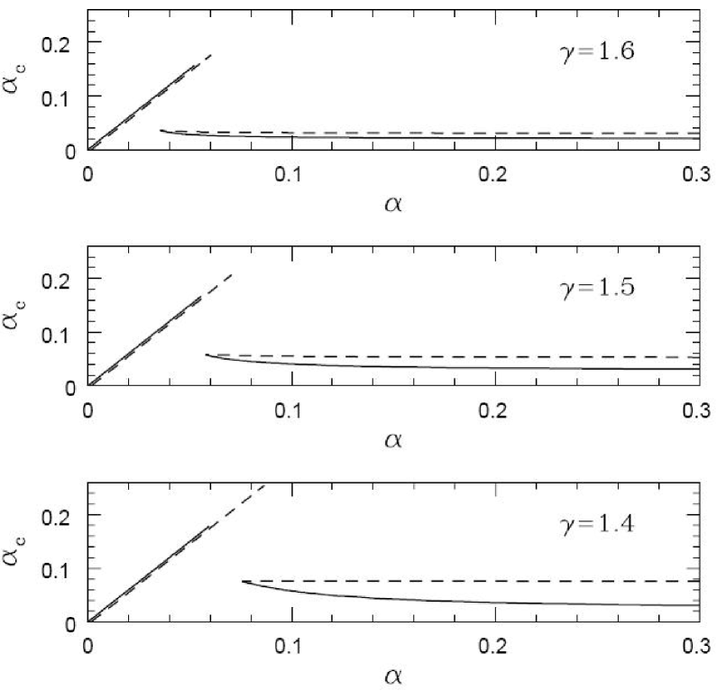
Figure 2.2: Variation of the convective parameter $\alpha_{c}$ as a function of the viscosity parameter $\alpha$ for three values the adiabatic index $\gamma$ (Narayan et al. 2000).

Self-similar solutions for ADAF with large-scale magnetic fields have also been studied (e.g.,Shadmehri 2004; Shadmehri & Khajenabi 2005; Akizuki & Fukue 2006; Shadmehri & Khajenabi 2006; Ghanbari, Salehi & Abbassi 2007; Zhang & Dai 2008b; Bu, Yuan & Xie 2009). The physical properties of magnetized flows are different to that without magnetic fields. For example, Akizuki & Fukue (2006) examined the effects of toroidal magnetic fields and mass-loss from the disk. They found that the disk becomes thick due to the magnetic pressure, and the radial infalling velocity and rotation becomes fast. Zhang & Dai (2008b) also discussed the self-similar solutions for CDAFs with large-scale fields. We will discuss these results in §3 in details.

2.5 NDAFs and Neutrino-Cooled Disks I: Formulae

If the accreting matter has a sufficiently high temperature and density, the photon optical depth is enormous and radiation cannot escape. However, it can cooled by neutrino emission, leading to a neutrino-dominated accretion flow (NDAF, Popham, Woosley & Fryer 1999).

Neutrino-cooled accretion disk around BH has been considered as the central engine of GRBs. Both processes of massive star collapses or compact object mergers lead to the formation of BH + neutrino-cooled disk systems. These disk are typically compact, with the bulk of the mass residing with $4\times 10^{7}$ cm of the BH ($\sim 3-5M_{\odot}$) and temperature ($10^{9}\textrm{K}\leq T\leq 10^{11}\textrm{K}$), density ($10^{9}$ g cm^-3$\leq\rho\leq$ $10^{11}$ g cm^-3), and a huge accretion rate up to $\sim 1M_{\odot}$ s^-1. The accretion timescale of these disks $t_{\rm acc}\sim M_{\rm disk}/\dot{M}$ is short, from tens of milliseconds after mergers to tens of seconds after collapses.

Neutrino Cooling Rates and Optical Depths

The generated viscosity can be cooled via neutrino emission via various cooling processes, including absorption processes such as electron-positron pair annihilation, electron-positron capture rate by nucleons, nucleon-nucleon bremsstrahlung, plasmon decay into neutrinos, and scattering processes such as neutrino-nucleon scattering and neutrino-electron scattering.

The rates of electron-positron pair annihilation into neutrinos are (Burrows & Thompson 2004)

$$q^{-}_{e^{-}e^{+}\rightarrow\nu_{e}\bar{\nu}_{e}}=2.56\times 10^{33}T_{11}^{9}f(\eta_{e})\,\textrm{ergs}\,\textrm{cm}^{-3}\,\textrm{s}^{-1},$$ (2.73)

$$q^{-}_{e^{-}e^{+}\rightarrow\nu_{\mu}\bar{\nu}_{\mu}}=q^{-}_{e^{-}e^{+}\rightarrow\nu_{\tau}\bar{\nu}_{\tau}}=1.09\times 10^{33}T_{11}^{9}f(\eta_{e})\,\textrm{ergs}\,\textrm{cm}^{-3}\,\textrm{s}^{-1},$$ (2.74)

where $T_{11}=T/10^{11}$ K,

$$f(\eta_{e})=\frac{F_{4}(\eta_{e})F_{3}(-\eta_{e})+F_{4}(-\eta_{e})F_{3}(\eta_{e})}{2F_{4}(0)F_{3}(0)}$$ (2.75)

and

$$F_{n}(\eta_{e})=\int_{0}^{\infty}\frac{x^{n}}{e^{x\mp\eta_{e}}+1}dx.$$ (2.76)

The electron-positron capture rate by nucleons (or, the URCA reaction) is represented by the sum of three terms:

$$q_{eN}=q_{p+e^{-}\rightarrow n+\nu_{e}}+q_{n+e^{-}\rightarrow p+\bar{\nu}_{e}}+q_{n\rightarrow p+e^{-}+\bar{\nu}_{e}},$$ (2.77)

with

$$q_{p+e^{-}\rightarrow n+\nu_{e}}=\frac{G_{F}^{2}C_{V}^{2}(1+3g_{A}^{2})}{2\pi^{3}\hbar^{7}c^{6}}n_{p}\int_{Q}^{\infty}dE_{e}E_{e}\sqrt{E_{e}^{2}-m_{e}^{2}c^{4}}(E_{e}-Q)^{3}\frac{1}{e^{(E_{e}-\mu_{e})/k_{B}T}+1},$$ (2.78)

$$q_{n+e^{-}\rightarrow p+\bar{\nu}_{e}}=\frac{G_{F}^{2}C_{V}^{2}(1+3g_{A}^{2})}{2\pi^{3}\hbar^{7}c^{6}}n_{n}\int_{m_{e}c^{2}}^{\infty}dE_{e}E_{e}\sqrt{E_{e}^{2}-m_{e}^{2}c^{4}}(E_{e}+Q)^{3}\frac{1}{e^{(E_{e}+\mu_{e})/k_{B}T}+1},$$ (2.79)

$$q_{n\rightarrow p+e^{-}+\bar{\nu}_{e}}=\frac{G_{F}^{2}C_{V}^{2}(1+3g_{A}^{2})}{2\pi^{3}\hbar^{7}c^{6}}n_{n}\int_{m_{e}c^{2}}^{Q}dE_{e}E_{e}\sqrt{E_{e}^{2}-m_{e}^{2}c^{4}}(Q-E_{e})^{3}\left(1-\frac{1}{e^{(E_{e}-\mu_{e})/k_{B}T}+1}\right),$$ (2.80)

where the constants $G_{F}=1.463\times 10^{-49}$ ergs cm^-3, $C_{V}^{2}=0.947$, axial vector $g_{A}=1.26$, $Q$ is defined as $(m_{n}-m_{p})c^{2}$, and $n_{p}$ and $n_{n}$ are the number density of protons and neutrons in the flows.

The nucleon-nucleon bremsstrahlung rate through $n+n\rightarrow n+n+\nu+\bar{\nu}$ is represented by

$$q^{-}_{\rm brems}=3.4\times 10^{33}T_{11}^{8}\rho_{13}^{1/3}\,\textrm{ergs}\,\textrm{cm}^{-3}\,\textrm{s}^{-1},$$ (2.81)

in the degeneracy regime of nucleons, and

$$q^{-}_{\rm brems}=1.5\times 10^{33}T_{11}^{5.5}\rho_{13}^{2}\,\textrm{ergs}\,\textrm{cm}^{-3}\,\textrm{s}^{-1},$$ (2.82)

in the nondegeneracy regime of nucleons (Hannestad & Raffelt 1998). Here $\rho_{13}=\rho/10^{13}$ g cm^-3.

Plasmon decay into neutrino through $\tilde{\gamma}\rightarrow\nu_{e}+\bar{\nu}_{e}$ is estimated as (Ruffert et al. 1996)

$$q^{-}_{\rm plasmon}=1.5\times 10^{32}T_{11}^{9}\gamma_{p}^{6}e^{-\gamma_{p}}(1+\gamma_{p})\left(2+\frac{\gamma_{p}^{2}}{1+\gamma_{p}}\right)\,\textrm{ergs}\,\textrm{cm}^{-3}\,\textrm{s}^{-1},$$ (2.83)

where $\gamma_{p}=5.656\times 10^{-2}[(\pi^{2}+3\eta_{e}^{2})/3]^{1/2}$. However, in most cases, both the $n-n$ bremsstrahlung and plasmon decay are less important than URCA and $e^{-}e^{+}$ pair annihilation in a NDAF. Thus, the absorption optical depths for three different types of neutrino can be calculated by (e. g., Popham et al. 1999; Kohri et al. 2005)

$$\tau_{a,\nu_{e}}=\frac{(q^{-}_{eN}+q^{-}_{e^{-}e^{+}\rightarrow\nu_{e}\bar{\nu}_{e}}+q^{-}_{\rm brems}+q^{-}_{\rm plasmon})H}{4(7/8\sigma_{B}T^{4})}\approx\frac{(q^{-}_{eN}+q^{-}_{e^{-}e^{+}\rightarrow\nu_{e}\bar{\nu}_{e}})H}{4(7/8\sigma_{B}T^{4})}$$ (2.84)

$$\tau_{a,\nu_{\mu,\tau}}=\frac{(q^{-}_{e^{-}e^{+}\rightarrow\nu_{\mu}\bar{\nu}_{\mu}}+q^{-}_{\rm brems})H}{4(7/8\sigma_{B}T^{4})}\approx\frac{q^{-}_{e^{-}e^{+}\rightarrow\nu_{\mu}\bar{\nu}_{\mu}}H}{4(7/8\sigma_{B}T^{4})}$$ (2.85)

Furthermore, the neutrino scattering processes include elastic scattering off background nucleons, $\nu_{i=e,\mu,\tau}+\{p,\>n\}\rightarrow\nu_{i=e,\mu,\tau}+\{p,\>n\}$. The total $\nu_{i}-p$ scattering cross section (Burrows & Thompson 2004)

$$\sigma_{p}=\frac{\sigma_{0}}{4}\left(\frac{\varepsilon_{\nu}}{m_{e}c^{2}}\right)^{2}[(C_{V}-1)^{2}+3g_{A}^{2}(C_{A}-1)^{2}],$$ (2.86)

and the transport cross section is

$$\sigma_{p}^{tr}=\frac{\sigma_{0}}{6}\left(\frac{\varepsilon_{\nu}}{m_{e}c^{2}}\right)^{2}[(C_{V}-1)^{2}+5g_{A}^{2}(C_{A}-1)^{2}],$$ (2.87)

where $\sigma_{0}=1.705\times 10^{-44}$ cm², $\varepsilon_{\nu}$ is the average neutrino energy. The total $\nu_{i}-n$ scattering cross section is

$$\sigma_{n}=\frac{\sigma_{0}}{4}\left(\frac{1+3g_{A}^{2}}{4}\right),$$ (2.88)

and the transport cross section is

$$\sigma_{n}^{tr}=\frac{\sigma_{0}}{4}\left(\frac{1+5g_{A}^{2}}{6}\right),$$ (2.89)

Neutrino-electron scattering rate is given by Tubbs & Schramm (1975) for electrons with different physical properties: (a) relativistic, nondegenerate electrons:

$$\sigma_{e\nu_{e}}=\frac{3}{8}\sigma_{0}\frac{\varepsilon_{\nu}}{m_{e}c^{2}}k_{B}T[(C_{V}+C_{A})^{2}+(C_{V}-C_{A})^{2}/3],$$ (2.90)

(b) relativistic degenerate electrons, and high energy neutrinos $\varepsilon_{\nu}\gg\varepsilon_{F}$ (Fermi energy of degenerate electrons):

$$\sigma_{e\nu_{e}}=\frac{3}{32}\sigma_{0}\frac{\varepsilon_{\nu}\varepsilon_{F}}{m_{e}c^{2}}[(C_{V}+C_{A})^{2}+(C_{V}-C_{A})^{2}/3],$$ (2.91)

(c) relativistic degenerate electrons, and low energy neutrinos $\varepsilon_{\nu}\ll\varepsilon_{F}$

$$\sigma_{e\nu_{e}}=\frac{1}{32}\sigma_{0}\left(\frac{\varepsilon_{\nu}}{m_{e}c^{2}}\right)^{2}\left(\frac{\varepsilon_{\nu}}{\varepsilon_{F}}\right)[(C_{V}+C_{A})^{2}+(C_{V}-C_{A})^{2}/3],$$ (2.92)

As a result, the neutrino scattering optical depth, which is contributed by neutrino-nucleon scattering and neutrino-electron, is given by

$$\tau_{s,\nu_{i}(e,\mu,\tau)}=H[\sigma_{p,\nu_{i}}n_{p}+\sigma_{n,\nu_{i}}n_{n}+\sigma_{e,\nu_{i}}(n_{e^{-}}+n_{e^{+}})]$$ (2.93)

Using the formulae of neutrino optical depths (2.84), (2.85) and (2.93) above, the total neutrino cooling rate per unit area is (Popham & Narayan 1995; Di Matteo et al. 2002)

$$Q^{-}_{\nu}=\sum_{i=e,\mu,\tau}\frac{(7/8)\sigma_{B}T^{4}}{(3/4)[\tau_{\nu_{i}}/2+1/\sqrt{3}+1/(3\tau_{a,\nu_{i}})]}$$ (2.94)

where the total optical depth of the neutrino is $\tau_{\nu_{i}}=\tau_{a,\nu_{i}}+\tau_{s,\nu_{i}}$. Formula (2.94) is designed to operate in both the optically very thin and optically very thick limits.

Thermodynamics

The cooling term in energy equation (2.20) has two contributions: neutrino emission (see formula 2.94) and photodisintegration of $\alpha$-particles

$$Q^{-}=Q^{-}_{\nu}+Q^{-}_{\rm photodis},$$ (2.95)

where

$$Q_{\rm photodis}=6.8\times 10^{38}\,\textrm{ergs}\,\textrm{cm}^{-3}\,\textrm{s}^{-1}\rho\left(\frac{A}{4}\right)^{-1}\left(\frac{B}{28.3\textrm{Mev}}\right)\left(\frac{v_{r}}{\textrm{cm}\,\textrm{s}^{-1}}\right)\left(\frac{dX_{nuc}/dr}{\textrm{cm}^{-1}}\right)$$ (2.96)

with $A$ being the mass number of the nucleons, $B$ being the binding energy of the nucleons (=28.3 Mev for ⁴He) and $X_{nuc}$ being the mass fraction of free nucleons

$$X_{nuc}=\textrm{min}\{1,\quad 295.5\rho_{10}^{-3/4}T_{11}^{9/8}\textrm{exp}(-0.8209/T_{11})\}.$$ (2.97)

The effect of photodisintegration can be neglected in the region with sufficiently high temperature and rare $\alpha$-particles $X_{nuc}\approx 1$.

The advection term in energy equation (2.20) is (Di Matteo et al. 2002; Liu et al. 2007)

$$Q_{\rm adv} = \rho v_{r}HT\frac{ds}{dr}$$ (2.98)

$$\approx\xi v_{r}\frac{H}{r}T\left(\frac{4}{3}a_{B}T^{4}+\frac{3}{2}\rho\Re\frac{1+3X_{nuc}}{4}+\frac{4}{3}\frac{u_{\nu}}{T}\right),$$

where $\xi\propto-d\textrm{ln}s/d\textrm{ln}r$ can be approximately taken as equal to 1. Another expression of $Q_{\rm adv}$ can be seen in Zhang & Dai (2008a) that

$$Q_{\rm adv}\approx\frac{\dot{M}T}{4\pi r^{2}}\left[\frac{\Re}{2}(1+Y_{e})\left(\frac{1+3X_{nuc}}{4}\right)+\frac{4}{3}g_{*}\frac{aT^{3}}{\rho}+\frac{4}{3}\frac{u_{\nu}}{T}\right],$$ (2.99)

where $Y_{e}$ is the radio of electron to nucleon number density, the parameter $g_{*}=2$ for photons and $g_{*}=11/2$ for a plasma of photons together with relativistic $e^{-}-e^{+}$ pairs.

The total pressure in the disk is

$$p=p_{e}+p_{\rm rad}+p_{\rm gas}+p_{v}.$$ (2.100)

The pressure $p_{e}$ is contributed by electrons and positrons $p_{e}=p_{e^{-}}+p_{e^{+}}$ with

$$p_{e^{\pm}}=\frac{1}{3}\frac{m_{e}^{4}c^{5}}{\pi^{2}\hbar^{3}}\int^{\infty}_{0}\frac{x^{4}}{\sqrt{x^{2}+1}}\frac{dx}{e^{(m_{e}c^{2}\sqrt{x^{2}+1}\mp\mu_{e})/k_{B}T}+1},$$ (2.101)

where $\mu_{e}$ is the chemical potential of the electron gas. The radiation pressure is

$$p_{\rm rad}=a_{B}T^{4}/3,$$ (2.102)

while Popham et al. (1999), Narayan et al. (2001), Di Matteo et al. (2002) took $p_{\rm rad}=11a_{B}T^{4}/12$, which include the contribution of relativistic $e^{-}-e^{+}$ pairs. We calculate the pressure of $e^{-}-e^{+}$ pairs in the term of $P_{e}$, not $P_{\rm rad}$. Moreover, The gas pressure, can be written as

$$p_{\rm gas}=\rho\Re T\left(\frac{1+3X_{nuc}}{4}\right),$$ (2.103)

as ideal gas pressure is still a good approximation in the neutrino-cooled disks. A more elaborate expression considered the series correction is (Janiuk et al. 2007)

$$p_{i(p,n)}=\frac{2\sqrt{2}}{3\pi^{2}}\frac{(m_{i}c^{2})^{4}}{(\hbar c)^{3}}\beta_{i}^{5/2}[F_{3/2}(\eta_{i},\beta_{i})+\beta_{i}F_{5/2}(\eta_{i},\beta_{i})/2],$$ (2.104)

where $\beta_{i}=kT/m_{e}c^{2}$, $\eta_{i}=\mu_{i}/k_{B}T$ with $\mu_{i}$ being the chemical potential, and $F_{k}(\eta_{i},\beta_{i})$ is the incomplete Fermi-Dirac integral for an index $k$. The pressure of neutrinos $p_{\nu}=u_{\nu}/3$, on the other hand, can be neglected in neutrino-cooled disks for most cases.

Charge Equilibrium and Chemical Equilibrium

The charge equilibrium requires

$$n_{p}=\frac{\rho Y_{e}}{m_{B}}=n_{e^{-}}-n_{e^{+}},$$ (2.105)

where

$$n_{e^{\mp}}=8\pi\left(\frac{m_{e}c}{h}\right)^{3}\int_{0}^{\infty}x^{2}dx\frac{dx}{e^{(m_{e}c^{2}\sqrt{x^{2}+1}\mp\mu_{e})/k_{B}T}+1},$$ (2.106)

The chemical equilibrium requires

$$n_{p}(\Gamma_{p+e^{-}\rightarrow n+\nu_{e}}+\Gamma_{p+\bar{\nu}_{e}\rightarrow n+e^{+}}+\Gamma_{p+e^{-}+\bar{\nu}_{e}\rightarrow n})$$

$$=n_{n}(\Gamma_{n+e^{+}\rightarrow p+\bar{\nu}_{e}}+\Gamma_{n\rightarrow p+e^{-}+\nu_{e}}+\Gamma_{n+\nu_{e}\rightarrow p+e^{-}})$$ (2.107)

We define a coefficient $K$ equal to $G_{F}^{2}C_{V}^{2}(1+3g_{A}^{2})/2\pi^{3}\hbar^{7}c^{6}$, then the transition reaction rates from neutrons to protons and from protons to neutrons are

$$\Gamma_{p+e^{-}\rightarrow n+\nu_{e}}=K\int_{Q}^{\infty}dE_{e}E_{e}\sqrt{E_{e}^{2}-m_{e}^{2}c^{4}}(E_{e}-Q)^{2}f_{e^{-}},$$ (2.108)

$$\Gamma_{p+e^{-}\leftarrow n+\nu_{e}}=K\int_{Q}^{\infty}dE_{e}E_{e}\sqrt{E_{e}^{2}-m_{e}^{2}c^{4}}(E_{e}-Q)^{2}(1-f_{e^{-}}),$$ (2.109)

$$\Gamma_{n+e^{+}\rightarrow p+\bar{\nu}_{e}}=K\int_{m_{e}c^{2}}^{\infty}dE_{e}E_{e}\sqrt{E_{e}^{2}-m_{e}^{2}c^{4}}(E_{e}+Q)^{2}f_{e^{+}},$$ (2.110)

$$\Gamma_{n+e^{+}\leftarrow p+\bar{\nu}_{e}}=K\int_{m_{e}c^{2}}^{\infty}dE_{e}E_{e}\sqrt{E_{e}^{2}-m_{e}^{2}c^{4}}(E_{e}+Q)^{2}(1-f_{e^{+}}),$$ (2.111)

$$\Gamma_{n\rightarrow p+e^{-}+\nu_{e}}=K\int_{m_{e}c^{2}}^{Q}dE_{e}E_{e}\sqrt{E_{e}^{2}-m_{e}^{2}c^{4}}(Q-E_{e})^{2}(1-f_{e^{-}}),$$ (2.112)

$$\Gamma_{n\leftarrow p+e^{-}+\nu_{e}}=K\int_{m_{e}c^{2}}^{Q}dE_{e}E_{e}\sqrt{E_{e}^{2}-m_{e}^{2}c^{4}}(Q-E_{e})^{2}f_{e^{-}},$$ (2.113)

where $f_{e^{\mp}}=\{\textrm{exp}[(E_{e}-\mu_{e})/k_{B}T]+1\}^{-1}$. If the neutrinos are perfectly thermalized and have an ideal Fermi-Dirac distribution, we can simplify equation (2.107) as

$$\left(\frac{n_{n}}{n_{p}}\right)_{\rm Eq}=\textrm{exp}\left\{\frac{\mu_{e}-Q}{k_{B}T}\right\}$$ (2.114)

for the neutrino-opaque limit and (Yuan 2005)

$$\left(\frac{n_{n}}{n_{p}}\right)_{\rm Eq}=\textrm{exp}\left\{\frac{2\mu_{e}-Q}{k_{B}T}\right\}$$ (2.115)

for the neutrino-transparent limit. A combined form for both neutrino-opaque and transparent cases can be given by (Lee et al. 2005; Liu et al. 2007)

$$\textrm{ln}\left(\frac{n_{n}}{n_{p}}\right)_{\rm Eq}=f(\tau_{\nu})\left\{\frac{2\mu_{e}-Q}{k_{B}T}\right\}+[1-f(\tau_{\nu})]\left\{\frac{\mu_{e}-Q}{k_{B}T}\right\}$$ (2.116)

Let us give a brief summary in this section. We have list all the formulae and equations for determining the structure of neutrino-cooled disks as functions of accretion rate $\dot{M}$, central BH mass $\dot{M}$, and the radius $r$ completely. The accretion disks satisfies the conservation equations (2.15), (2.16), (2.18) and (2.20). The total neutrino cooling rate is expressed as formula (2.94), while formulae (2.73) to (2.93) show how to calculate various cooling processes and neutrino optical depths. Photodisintegration is showed as formula (2.96), while advection flux can be estimated using formula (2.98) or (2.99). The total pressure is contributed by four terms as showed in equation (2.100), with formulae (2.101) to (2.104) discuss each type of pressure. Finally, we need the charge and chemical equilibrium equations (2.105) and (2.107), with density equation (2.106) and transition rates formulae (2.108) to (2.113).

Effects of Highly Strong Magnetic Fields

Now we discuss the neutrino-cooled disk with highly strong magnetic fields $\geq 10^{14}$ G. Such ultrahigh magnetic fields may be generated by amplification processes in disks such as differential rotation, or directly form the central BH. Strong magnetic fields could change the disk physical properties significantly. The effect of magnetic fields on macrophysical conservation equations have been discussed in §2.1.2 (see Xie et al. 2007 and Lei et al. 2008 for more discussion). Here er mainly focus on microphysics. The main modification in the case of strong magnetized disk comes from the available phase space for the electrons. The phase space for $B=0$ should be replaced as

$$\frac{2}{h^{3}}\int d^{3}p\longrightarrow\sum_{n=0}^{\infty}g_{nL}\int\frac{eB_{m}}{h^{2}c}dp_{z},$$ (2.117)

where the free degree $g_{nL}=1$ for $n=1$ and $g_{nL}=2$ for $n\geq 1$. Thus the energy of electron is

$$E=\sqrt{p_{z}^{2}c^{2}+m^{2}c^{4}+2n_{L}eB\hbar c},$$ (2.118)

which is the form of "Landau $n_{L}$-level of energy". The electron number density reads

$$n_{e^{\mp}}=\sum_{n=0}^{\infty}g_{nL}\int_{-\infty}^{\infty}dp\frac{eB_{m}}{h^{2}c}f_{e^{\mp}},$$ (2.119)

and the charge equilibrium condition satisfies

$$\frac{\rho Y_{e}}{m_{B}}=\sum_{n=0}^{\infty}g_{nL}\int_{-\infty}^{\infty}dp\frac{eB_{m}}{h^{2}c}(f_{e^{-}}-f_{e^{+}}).$$ (2.120)

The pressure of electrons and positrons is modified as

$$P_{e_{\mp}}=\sum_{n=0}^{\infty}g_{nL}\int_{-\infty}^{\infty}dp\frac{eB_{m}}{3h^{2}}\frac{p^{2}c}{\sqrt{p^{2}c^{2}+m^{2}c^{4}+2n_{L}eB_{m}\hbar c}}f_{e^{\mp}}.$$ (2.121)

The various neutrino cooling rates should also be modified under in strong magnetic fields environment. We give the examples of the $e^{-}-e^{+}$ capture rate, which is the most important cooling term in neutrino-cooled disks:

$$q_{p+e^{-}\rightarrow n+\nu_{e}}=\frac{G_{F}^{2}C_{V}^{2}(1+3a^{2})}{8\pi^{3}\hbar^{6}c^{5}}eB_{z}(m_{e}c^{2})^{4}\sum_{n=0}^{\infty}g_{nL}n_{p}\int\frac{\varepsilon(\varepsilon-q)^{3}d\varepsilon}{\sqrt{\varepsilon^{2}-1-2n_{L}eB_{m}\hbar c}}f_{e^{-}},$$ (2.122)

$$q_{n+e^{-}\rightarrow p+\bar{\nu}_{e}}=\frac{G_{F}^{2}C_{V}^{2}(1+3a^{2})}{8\pi^{3}\hbar^{6}c^{5}}eB_{z}(m_{e}c^{2})^{4}\sum_{n=0}^{\infty}g_{nL}n_{p}\int\frac{\varepsilon(\varepsilon+q)^{3}d\varepsilon}{\sqrt{\varepsilon^{2}-1-2n_{L}eB_{m}\hbar c}}f_{e^{+}},$$ (2.123)

$$q_{n\rightarrow p+e^{-}+\bar{\nu}_{e}}=\frac{G_{F}^{2}C_{V}^{2}(1+3a^{2})}{8\pi^{3}\hbar^{6}c^{5}}eB_{z}(m_{e}c^{2})^{4}\sum_{n=0}^{\infty}g_{nL}n_{p}\int\frac{\varepsilon(q-\varepsilon)^{3}d\varepsilon}{\sqrt{\varepsilon^{2}-1-2n_{L}eB_{m}\hbar c}}(1-f_{e^{-}}),$$ (2.124)

The above equations allows us to solve the structure of neutrino-cooled disks with ultrahighly magnetic fields.

2.6 NDAFs and Neutrino-Cooled Disks II: Solutions

Analytical Solutions

Popham, Woosley & Fryer (1999) first studied the structure of neutrino-cooled disks with huge accretion rate from $0.01M_{\odot}$ s^-1 to $10.0M_{\odot}$ s^-1. They simplified the formulae of neutrino cooling emission (2.73), (2.77) in last section as

$$q_{\nu\bar{\nu}}\approx 5.0\times 10^{33}T_{11}^{9}\,\textrm{ergs}\,\textrm{cm}^{-3}\,\textrm{s}^{-1}$$ (2.125)

for pair annihilation, and

$$q_{eN}\approx 9.0\times 10^{33}\rho_{10}T_{11}^{6}X_{nuc}\,\textrm{ergs}\,\textrm{cm}^{-3}\,\textrm{s}^{-1}$$ (2.126)

for the capture of pairs on nucleons. Thus the neutrino cooling rate over a half-thickness disk can be written as

$$Q_{\nu}^{-}=(q_{\nu\bar{\nu}}+q_{eN})H.$$ (2.127)

Moreover, the pressure of electrons is assumed mainly due to relativistic degenerate electrons; $P_{e}\propto(\rho_{e}Y)^{4/3}$ with $Y_{e}$ being fixed as 0.5. Based on these simplifications, Narayan, Piran & Kumar (2001) derived the analytical solutions of NDAFs. They took the disk mass ($m_{d}M_{\odot}$) and the outer radius ($r_{out}R_{S}$, $R_{S}$ is the Schwarzschild radius of the central BH). GRBs could only be produced when the disk is small enough, i.e., $r_{out}<118\alpha_{-1}^{-2/7}m_{3}^{-1}m_{d}^{3/7}$ with $\alpha_{-1}=\alpha/0.1$, $m_{3}=M/(3M_{\odot})$ and $\dot{m}=\dot{M}/M_{\odot}\,\textrm{s}^{-1}$, because small disk can be sufficiently cooled via neutrino emission and accreted most of its mass into the central BH. On the other hand, large accretion disk with its CDAF structure are unlikely to produce GRBs since very little cooling mass reaches the BH. When the outer radius satisfies $26.2\alpha_{-1}^{-2/7}m_{3}^{-46/49}m_{d}^{20/49}<r_{out}<118\alpha_{-1}^{-2/7}m_{3}^{-1}m_{d}^{3/7}$, gas pressure dominates in the NDAF. As a result, the temperature, accretion timescale and accretion rate of the disk are

$$T_{11}=0.548\alpha_{-1}^{1/5}m_{3}^{-1/5}r^{-3/10},$$

$$t_{acc}=2.76\times 10^{-2}\alpha_{-1}^{-6/5}m_{3}^{6/5}r_{out}^{4/5},$$

$$\dot{m}=36.2\alpha_{-1}^{6/5}m_{3}^{-6/5}m_{d}r_{out}^{-4/5}.$$ (2.128)

When $r_{out}<26.2\alpha_{-1}^{-2/7}m_{3}^{-46/49}m_{d}^{20/49}$, electron degeneracy pressure takes over from gas pressure and the disk quantities are

$$T_{11}=0.800\alpha_{-1}^{1/6}m_{3}^{-13/42}m_{d}^{1/21}r^{-5/12},$$

$$t_{acc}=2.82\times 10^{-3}\alpha_{-1}^{-1}m_{3}^{13/7}m_{d}^{-2/7}r_{out}^{3/2},$$

$$\dot{m}=355\alpha_{-1}m_{3}^{-13/7}m_{d}^{9/7}r_{out}^{-3/2}.$$ (2.129)

However, these solutions are derived based on the assumption that the accreting gas is neutrino optically thin. Since the NDAF may become neutrino optically thick when $r<20.5\alpha_{-1}^{-4/17}m_{3}^{-110/119}m_{d}^{46/119}$. Inside the radius, neutrino transport should be considered.

The accretion timescale $t_{acc}$ is sensitive dependence on the viscosity parameter $\alpha$. However, the accretion timescale is unlikely to be sufficiently long to explain long GRBs, because the above discussions are based on the scenario that the disk or debris torus is formed after mergers immediately without supplementary feeding material. If the accretion disk can be fed by fallback of material after the collapse of a massive star, as in the collapsar model, then the timescale of the burst id determined by fallback, not accretion. Such a disk can produce long GRBs. On the other hand, as showed in numerical calculations, a disk with a fixed huge hyperaccretion rate may contains different regions such as convection-dominated region, neutrino-dominated and gas-pressure-dominated or degeneracy-pressure-dominated region at the same time. This scenario is different to that in Narayan et al. (2001) that a disk is either CDAF or NDAF, depending on its size and total mass.

Kohri & Mineshige (2002) used semi-analytical method to study NDAFs with high surface density $\Sigma\geq 10^{20}$ g cm^-2, which is realized when about a solar mass of accreting matter is contained within a disk of size $\sim 5\times 10^{6}$ cm. Electron degeneracy pressure dominates over gas and radiation pressure. This result is consistent with that in Narayan et al. (2001). On the other hand, Kohri & Mineshige (2002) also showed the discrepancies between their results and those in Narayan et al. (2001). For example, the relation $p_{\rm rad}\gg p_{\rm gas}$ is always realized in the nondegenerate electron region at $T\geq m_{e}c^{2}/k_{B}$, while Narayan et al. (2001) showed $p_{\rm gas}>p_{\rm rad}$ in this region. More elaborate numerical calculations (e.g., Kohri et al. 2005) support the analytical result of Kohri & Mineshige (2002). Table 2.1 gives the five cases for $T-\Sigma$ and $\dot{M}-\Sigma$ relations from Kohri & Mineshige (2002).

Region	$p$	$Q^{+}_{\rm vis}$	$Q^{-}_{\nu}$	$T-\Sigma$ relation	$\dot{M}-\Sigma$ relation
I	$p_{\rm gas}$	$\alpha\Sigma Tr^{-3/2}M^{1/2}$	$Q_{\rm rad}^{-}\propto\Sigma^{-1}T^{4}$	$\alpha^{1/3}\Sigma^{2/3}r^{-1/2}M^{1/6}$	$\alpha^{4/3}\Sigma^{5/3}rM^{-1/3}$
II	$p_{\rm rad}$	$\alpha\Sigma^{-1}T^{8}r^{3/2}M^{-1/2}$	$Q_{\rm rad}^{-}\propto\Sigma^{-1}T^{4}$	$\alpha^{-1/4}\Sigma^{0}r^{-3/8}M^{1/6}$	$\alpha^{-1}\Sigma^{-1}r^{3/2}M^{-1/2}$
III	$p_{\rm rad}$	$\alpha\Sigma^{-1}T^{8}r^{-3/2}M^{-1/2}$	$Q_{\rm adv}^{-}\propto\alpha\Sigma^{-3}T^{16}r^{11/2}M^{-5/2}$	$\alpha^{0}\Sigma^{1/4}r^{-1/2}M^{1/4}$	$\alpha\Sigma r^{1/2}M^{1/2}$
IV	$p_{\rm d,rel}$	$\alpha\Sigma^{9/7}Tr^{-27/14}M^{9/14}$	$Q_{\rm adv}^{-}\propto\alpha\Sigma T^{2}r^{-1/2}M^{-1/2}$	$\alpha^{0}\Sigma^{1/7}r^{-5/7}M^{4/7}$	$\alpha\Sigma^{9/7}r^{15/14}M^{-5/14}$
V	$p_{\rm d,rel}$	$\alpha\Sigma^{9/7}Tr^{-27/14}M^{9/14}$	$Q_{\nu}^{-}\propto\eta_{e}^{9}T^{9}\Sigma^{1/7}r^{9/7}M^{-3/7}$	$\Sigma^{4/7}r^{-6/7}M^{2/7}$	$\alpha\Sigma^{9/7}r^{15/14}M^{-5/14}$

Table 2.1: $T-\Sigma$ and $\dot{M}-\Sigma$ relations in various regions. Here $p$ shows the dominant type of pressure. $p_{\rm d,rel}$ is the electron relativistic degeneracy pressure (Kohri & Mineshige 2002).

Zhang & Dai (2008a) also obtained a group of analytical solutions both for ADAF we do not consider the effect of convection) and NDAF region in a disk with fixed accretion rate. The disk region for a radiation-pressure-dominated ADAF is

$$r_{6}f^{1/5}>2.28m^{-3/5}\dot{m}_{d}^{6/5}\alpha_{-1}^{-2},$$

$$r_{6}f^{-7/3}<74.6\left(1+Y_{e}\right)^{-8/3}m^{7/3}\dot{m}_{d}^{-2/3}\alpha_{-1}^{2/3},$$

$$r_{6}f^{-7/3}<74.6\left(1+Y_{e}\right)^{-8/3}m^{7/3}\dot{m}_{d}^{-2/3}\alpha_{-1}^{2/3},$$ (2.130)

where the notations in these relations are slightly different to those in Narayan et al. (2001): $\dot{M}=0.01\dot{m}_{d}M_{\odot}$ s^-1, $M=1.4mM_{\odot}$, $r=10^{6}r_{6}$ cm. Also, the gas-pressure-dominated ADAF region satisfies

$$r_{6}^{47/22}f^{-20/11}>128\left(1+Y_{e}\right)^{-26/11}m^{29/22}\dot{m}_{d}^{10/11}\alpha_{-1}^{-21/11},$$

$$r_{6}f^{-7/3}>74.6\left(1+Y_{e}\right)^{-8/3}m^{7/3}\dot{m}_{d}^{-2/3}\alpha_{-1}^{2/3}.$$ (2.131)

The neutrino-cooled dominated region, where satisfies $Q_{\rm adv}<Q_{\nu}^{-}$ is

$$r_{6}^{47/22}f^{-20/11}<128\left(1+Y_{e}\right)^{-26/11}m^{29/22}\dot{m}_{d}^{10/11}\alpha_{-1}^{-21/11},$$ (2.132)

and the gas-pressure-dominated NDAF is the region where

$$r_{6}f^{-20/33}>3.18Y_{e}^{80/33}\left(1+Y_{e}\right)^{-36/11}m^{1/3}\dot{m}_{d}^{20/33}\alpha_{-1}^{-38/33},$$

$$r_{6}f^{-20/33}<6.90\alpha_{-1}^{-38/33}f^{20/33}m^{1/3}\dot{m}_{d}^{20/33}(1+Y_{e})^{-28/33}.$$ (2.133)

Finally, we derived the region where is degeneracy-pressure-dominated NDAF

$$r_{6}f^{-7/3}>8.07\times 19^{3}m^{7/3}\dot{m}_{d}^{-2/3}\alpha_{-1}^{2/3}Y_{e}^{-44/3}\left(1+Y_{e}\right)^{12}\alpha_{-1}^{-38/33},$$

$$r_{6}f^{-7/3}>174m^{7/3}\alpha_{-1}^{2.3}\dot{m}_{d}^{-2/3}Y_{e}^{-8/3},$$ (2.134)

which could only be satisfied for very large radius.

On the other hand, for a fixed radius $r$, we could obtain the range of $\dot{m}_{d}$ for two types of accretion flows with various dominated pressure. More details about the analytical solutions of neutrino-cooled disk will be discussed in §3.3.1.

Numerical Solutions

Numerical methods have been carried out to study the neutrino-cooled disks first by Popham et al. (1999), then by Di Matteo et al. (2002), Lee & Ramirez-Ruiz (2002), Lee et al. (2004, 2005), Janiuk et al. (2004, 2007), Kohri et al. (2005), Gu et al. (2006), Chen & Beloborodov (2007), Liu et al. (2007), Shibata et al. (2007), etc. Their numerical outcomes are slightly different with each other, due to the different simplifications and energy transport forms.

Popham, Woosley & Fryer (1999) adopted the conservation equations based on Kerr geometry, but used simplified equations of neutrino emission and pressure mentioned above. They did not consider the effect of neutrino opacity. The disk is advection-dominated outside about $10^{8}$ cm, and neutrino-dominated inside. Di Matteo et al. (2002) followed Kohri & Mineshige (2002) to discuss various neutrino cooling processes, and focused on the effect of neutrino opacity at high $\dot{M}$. They found that, for $\dot{M}\geq 1M_{\odot}$ s^-1, neutrinos are sufficiently trapped that energy advection becomes the dominant cooling mechanism in the flow. Thus the neutrino luminosity would decrease for high accretion rate, and $\nu\bar{\nu}$ annihilation above the neutrino-cooled disk is an inefficient mechanism. Similar to Popham et al. (1999), they mainly considered the contribution of relativistic degeneracy pressure $p_{e}\propto(\rho Y_{e})^{4/3}$ in the term of electron pressure, and fix $Y_{e}$ to be 0.5 in their calculations. Gu et al. (2006), on the other hand, argued that in the optically thick region advection does not necessary dominate over neutrino cooling because the advection factor $f_{\rm adv}=Q_{\rm adv}/Q_{\rm vis}^{+}$ is relevant to the geometrical depth rather tan the optical depth of the flow (Abramowicz et al. 1986)

$$f_{\rm adv}\propto(H/r)^{2}.$$ (2.135)

This conclusion is consistent with the more elaborate numerical calculations by Kohri et al. (2005).

Kohri, Narayan & Piran (2005) calculated the electron pressure and density using the Fermi-Dirac distribution (2.101) and (2.106), and adopt the full equation (2.94) for neutrino cooling rate, thermal equation (2.114) for chemical equilibrium calculation. Figure 2.3 shows the contours of matter density $\rho_{10}=\rho/10^{10}$ g cm^-3, temperature $T_{11}=T/10^{11}$ K, the degeneracy parameter $\eta_{e}$ and the dominant cooling process in the radius-accretion rate parameter plane. Moreover, Figure 2.4 is the contour of the nucleon fraction $X_{nuc}$, neutrino-to-proton ratio, the dominant source of pressure and number density of electrons. These two figures well describe the physical properties of the Newtonian Keplerian neutrino-cooled disk from accretion rate less than $0.1M_{\odot}\,\textrm{s}^{-1}$ to $10^{3}M_{\odot}\,\textrm{s}^{-1}$ in the disk of size $\sim 6\times 10^{7}(M/M_{\odot})$ cm.

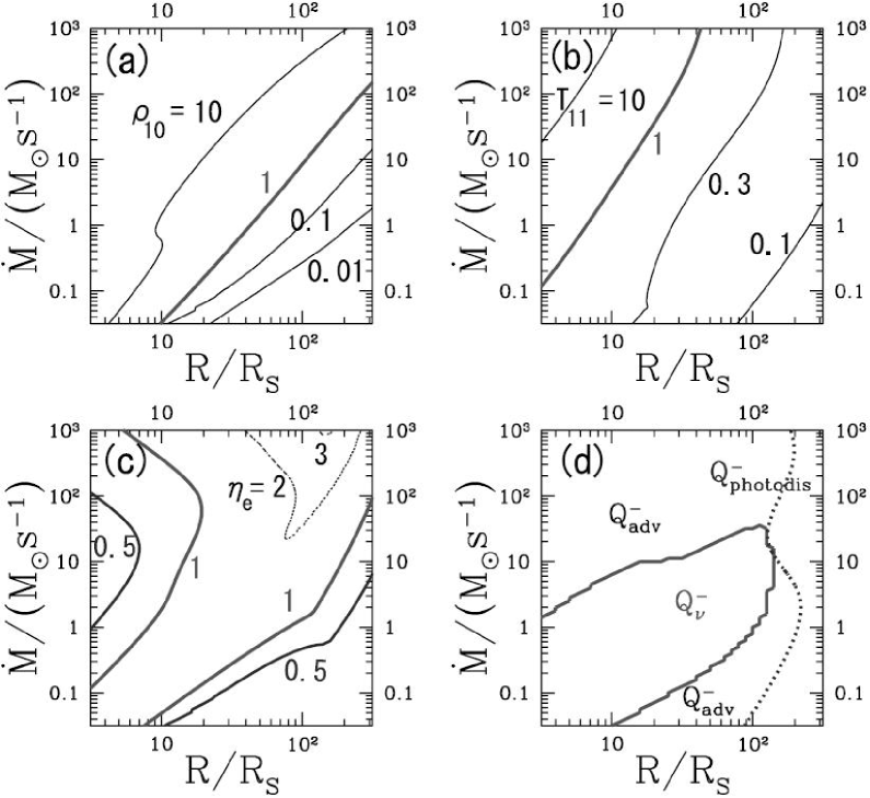
Figure 2.3: contours of matter density $\rho_{10}=\rho/10^{10}$ g cm^-3, temperature $T_{11}=T/10^{11}$ K, the degeneracy parameter $\eta_{e}$ and the dominant cooling process in the radius-accretion rate parameter plane (kohri et al. 2005).

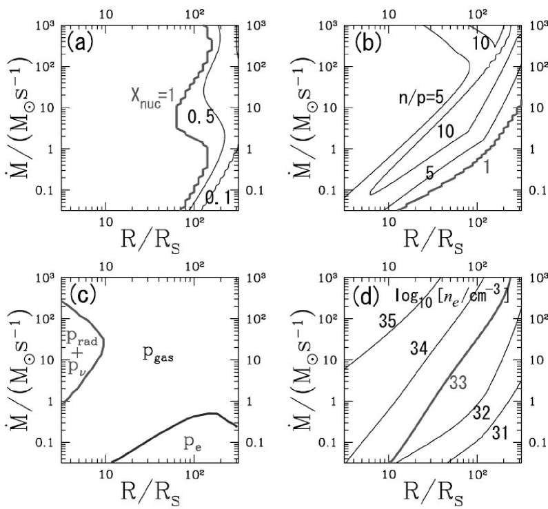
Figure 2.4: Contour of the nucleon fraction $X_{nuc}$, neutron-to-proton ratio, the dominant source of pressure and number density of electrons (kohri et al. 2005).

Similar to Popham et al. (1999), Chen & Beloborodov (2007) presented general relativistic calculation of macrophysical structure of neutrino-cooled disks around Kerr BHs. Also, they adopted Fermi-Dirac distributions to calculate the electron density and pressure. However, they only considered the $e^{-}-e^{+}$ pair capture onto nucleons among various neutrino cooling processes, and simplified the equations of neutrino transfer and total cooling rate. Figure 2.5 gives the scenario of an accretion disk around a Kerr BH with a huge accretion rate, where radius $r_{\alpha}$, $r_{\rm ign}$, $r_{\nu}$, $r_{\bar{\nu}}$, $r_{\rm tr}$ are five characteristic radii:

• Radius $r_{\alpha}$, where 50% of the $\alpha$-particles are decomposed into three nucleons via photodisintegration process.

• "Ignition" radius $r_{\rm ign}$, where the neutrino emission switches on, i.e., the accretion flow becomes neutrino-cooled. The ignition radius exists only if $\dot{M}>\dot{M}_{\rm ign}$, where the critical accretion rate $\dot{M}_{\rm ign}$ depends on the viscosity parameter $\alpha$ and spin parameter $a$.

• Radius $r_{\nu}$, where the disk becomes opaque for neutrinos and they relax to a thermal distribution.

• Radius $r_{\bar{\nu}}$, where the disk becomes opaque for antineutrinos. Then both neutrinos and antineutrinos are now in thermal equilibrium with the matter.

• Radius $r_{\rm tr}$, where the timescale of neutrino diffusion becomes longer than the accretion timescale, and neutrinos get rapped and advected into the black hole.

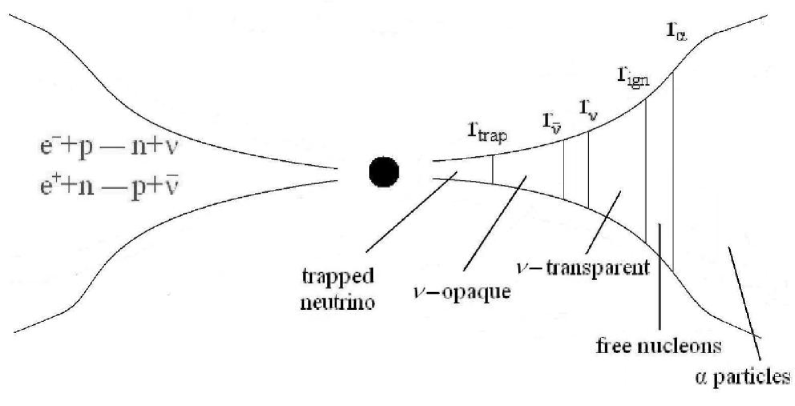
Figure 2.5:

2D and 3D time-dependent simulations were given by Lee & Ramirez-Ruiz (2002), Lee et al. (2004, 2005) and Setiawan et al. (2004). Lee & Ramirez-Ruiz (2002) took the disk initial condition from 3D BH-NS simulations and studied the time dependence of the disk structure for 0.2 s in 2D cylindrical coordinates ($r,z$). They showed the dynamical evolution of the accretion disks formed after BH-NS mergers. A neutrino-cooled disk could produce a short impulsive energy input $L_{\nu\bar{\nu}}\propto t^{-5/2}$ via $\nu\bar{\nu}$-annihilation, while strong fields $B\approx 10^{16}$ G being anchored in the dense matter could also power a short GRB. However, the equation of state was simplified in Lee & Ramirez-Ruiz (2002) with a ideal gas and adiabatic index $\Gamma=4/3$. Also, they assumed that all the energy dissipated by viscosity is radiated away. Next Lee et al. (2004) improved the equations of state following Popham et al. (1999) and Di Matteo et al. (2002), and considered pair capture on nucleons as the main neutrino cooling process. The improved simulations last approximately 1 s. The inclusion of neutrino optical depth effects produces important qualitative temporal and spatial transitions in the evolution and structure of the disk, which may directly reflect on the duration and variability of short GRBs. Later, more elaborate 2D simulations were carried out, also by Lee et al. (2005), who used much more details detailed equation of state, neutrino emission processes and optical depths. They construct the bridging formula for chemical equilibrium in both optical thin and thick cases (i.e., equation [2.115]). However, the effect of neutrino absorption was still neglected, since the total neutrino cooling luminosity is computed according

$$L_{\nu}=\int\rho^{-1}(q_{eN}+q_{e^{-}e^{+}}+q_{\rm brem}+q_{plasmon}).$$ (2.136)

Also, as conservation equations were not included, the initial conditions were also taken from the results of BH-NS merger simulations. Setiawan, Ruffert, & Janka (2004) presented 3D simulations of a time-dependent hyperaccretion disk around a BH, while the initial data is obtained from Janka et al. (1999) with a BH mass of $4.017M_{\odot}$ and torus mass changing from $0.0120M_{\odot}$ to $0.1912M_{\odot}$. The accretion duration in their model is about tens of milliseconds.

The above 2D and 3D simulations stared with initial disk conditions obtained from the early-phase simulations of compact stars merger, and focused on disk dynamical evolution less than 1 s. Janiuk et al. (2004) self-consistently obtained the initial disk structure based on the equations as showed in Popham et al. (1999), Di Matteo et al. (2002), Kohri et al. (2005); and extended the study of disk evolution to much longer timescale. The time-dependent evolution is mainly cased by density and temperature variation, which can be determined by time-dependent equations of mass and angular momentum conservation

$$\frac{\partial\Sigma}{\partial t}=\frac{1}{r}\frac{\partial}{\partial r}\left[3r^{1/2}\frac{\partial}{\partial r}(r^{1/2}\nu\Sigma)\right],$$ (2.137)

$$\frac{\partial T}{\partial t}+v_{r}\frac{\partial T}{\partial r}=\frac{T}{\Sigma}\frac{4-3\chi}{12-9\chi}\left(\frac{\partial\Sigma}{\partial t}+v_{r}\frac{\partial\Sigma}{\partial t}+v_{r}\frac{\partial\Sigma}{\partial r}\right)+\frac{T}{pH}\frac{1}{12-9\chi}(Q^{+}_{\rm vis}-Q^{-}_{\nu}),$$ (2.138)

where $\chi=(p-p_{\rm rad})/p$. Moreover, the contribution of photodisintegration varies with time as

$$Q_{\rm photo}^{-}\propto v_{r}\frac{\partial X_{nuc}}{\partial r}+\frac{\partial X_{nuc}}{\partial t}.$$ (2.139)

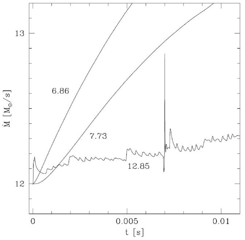
Figure 2.6: The evolution of local accretion, for several chosen radial locations in the disk: 6.87, 7.73 and 12.85 $R_{s}$. The starting accretion rate is $\dot{M}=12M_{\odot}$ s^-1 (Janiuk et al. 2007).

Janiuk et al. (2007) found that, for sufficiently large accretion rates ($\dot{M}\geq 10M_{\odot}$ s^-1, the inner regions of the disk develop a viscous and thermal instability, which might be relevant for GRB observations. For example, Figure 2.6 showed the behavior of the local accretion rate in the unstable disk at several chosen locations with the instability strip. Furthermore, Metzger, Piro & Quataert (2008) presented the dynamical evolution of the neutrino-cooled disks in a timescale of $\sim 100$ s based on their "ring model", which treats the disk as a single annulus that is evolved forward in time. They also obtained analytic self-similar time-depend solution that the disk mass $M_{d}\propto t^{-5/8}$, the accretion rate $\dot{M}\propto t^{-13/8}$ for neutrino-cooled thin disk, and $M_{d}\propto t^{-1/3}$, $\dot{M}\propto t^{-4/3}$ for late-time advective case.

2.7 Neutrino Annihilation and Jet Production

In neutrino-cooled disks and other compact high-energy objects, a significant fraction of the gravitational energy is converted during the accretion into neutrino flux. This energy is available to extracted via $\nu\bar{\nu}$-annihilation and subsequent pair production. The problem is that, could the process of $\nu\bar{\nu}$-annihilation launch a relativistic jet, and provide sufficient energy for a GRB? We have mentioned some results of $\nu\bar{\nu}$-annihilation above disks, now we discuss this process more detailed.

Motivated by the delayed explosion of Type II supernovae, the energy deposition rate due to the $\nu\bar{\nu}$-annihilation above the spherical neutrinosphere has been calculated by Cooperstein et al. (1986), Goodman et al. (1987), Berezinsky & Prilutsky (1987) and later by Salmonson & Wilson (1999). The $\nu\bar{\nu}\rightarrow e^{-}e^{+}$ deposition per unit time per volume in Newtonian case is (Goodman et al. 1987)

$$q_{\nu\bar{\nu}}(\textbf{r})=\int\int f_{\nu}(\textbf{p}_{\nu},\textbf{r})f_{\bar{\nu}}(\textbf{p}_{\bar{\nu}},\textbf{r})\{\sigma|\textbf{v}_{\nu}-\textbf{v}_{\bar{\nu}}|\varepsilon_{\nu}\varepsilon_{\bar{\nu}}\}\frac{\varepsilon_{\nu}+\varepsilon_{\bar{\nu}}}{\varepsilon_{\nu}\varepsilon_{\bar{\nu}}}\textrm{d}^{3}\textbf{p}_{\nu}\textrm{d}^{3}\textbf{p}_{\bar{\nu}},$$ (2.140)

where $f_{\nu}$ and $f_{\bar{\nu}}$ are the numbers of neutrinos and antineutrinos per unit volume per momentum state, $\textbf{v}_{\nu}$ is the velocity of the neutrino, and $\sigma$ is the appropriate rest-frame cross section, which can be calculated as

$$\{\sigma|\textbf{v}_{\nu}-\textbf{v}_{\bar{\nu}}|\varepsilon_{\nu}\varepsilon_{\bar{\nu}}\}=2\mathscr{K}G_{F}^{2}(\varepsilon_{\nu}\varepsilon_{\bar{\nu}}-\textbf{p}_{\nu}\cdot\textbf{p}_{\bar{\nu}}c^{2})^{2},$$ (2.141)

where $G_{F}^{2}=5.29\times 10^{-44}$ cm² Mev^-2 and

$$\mathscr{K}=\frac{1\pm 4\textrm{sin}^{2}\theta_{W}+8\textrm{sin}^{4}\theta_{W}}{6\pi},$$ (2.142)

with the plus sign being for $\nu_{e}\bar{\nu}_{e}$ pairs and minus sign being for $\nu_{\mu}\bar{\nu}_{\mu}$ and $\nu_{\tau}\bar{\nu}_{\tau}$ pairs, and $\textrm{sin}^{2}\theta_{W}\approx 0.23$. Taking $\textrm{d}^{3}\textbf{p}_{\nu}=(\varepsilon_{\nu}^{2}/c^{3})\textrm{d}\varepsilon_{\nu}\textrm{d}\varepsilon_{\nu}$, we obtain

$$q_{\nu\bar{\nu}}(\textbf{r})=\frac{2\mathscr{K}G_{F}^{2}}{c^{5}}\Theta(\textbf{r})\int\int f_{\nu}f_{\bar{\nu}}(\varepsilon_{\nu}+\varepsilon_{\bar{\nu}})\varepsilon_{\nu}^{3}\textrm{d}\varepsilon_{\nu}\varepsilon_{\bar{\nu}}^{3}\textrm{d}\varepsilon_{\bar{\nu}},$$ (2.143)

where the angular integration factor

$$\Theta(\textbf{r})=\int\int(1-\Omega_{\nu}\cdot\Omega_{\bar{\nu}})^{2}\textrm{d}\Omega_{\nu}\textrm{d}\Omega_{\nu}.$$ (2.144)

The phase factor integrations are

$$\int_{0}^{\infty}f_{\nu}\varepsilon_{\nu}^{3}\textrm{d}\varepsilon_{\nu}=\frac{2(k_{B}T)^{4}}{h^{3}}\frac{7\pi^{4}}{120},$$ (2.145)

$$\int_{0}^{\infty}f_{\nu}\varepsilon_{\nu}^{4}\textrm{d}\varepsilon_{\nu}=\frac{2(k_{B}T)^{5}}{h^{3}}\frac{45\zeta(5)}{2}.$$ (2.146)

Thus the $\nu\bar{\nu}$-annihilation energy deposition rate is

$$q_{\nu\bar{\nu}}(\textbf{r})=\frac{14\mathscr{K}G_{F}^{2}\pi^{4}\zeta(5)}{c^{5}h^{6}}(k_{B}T)^{9}\Theta(\textbf{r})\propto T^{9}\Theta(\textbf{r}),$$ (2.147)

where the angular integration can be analytically derived as

$$\Theta(\textbf{r})=\frac{2\pi^{3}}{3}(1-x)^{4}(x^{2}+4x+5)$$ (2.148)

with $x=\sqrt{1-(R_{\nu}/r)^{2}}$. Here $R_{\nu}$ is the radius of neutrinosphere. Goodman et al. (1987) estimated the total rate of annihilation energy input

$$Q(\nu_{e}\bar{\nu}_{e})=\int_{R_{\nu}}^{\infty}q(\nu_{e}\bar{\nu}_{e})4\pi r^{2}dr=0.682\times 10^{51}\,\textrm{ergs}\,\textrm{s}^{-1}$$

$$Q(\nu_{\mu}\bar{\nu}_{\mu})=Q(\nu_{\tau}\bar{\nu}_{\tau})=0.585\times 10^{51}\,\textrm{ergs}\,\textrm{s}^{-1}$$

$$Q({\rm total})=1.9\times 10^{51}\,\textrm{ergs}\,\textrm{s}^{-1}.$$ (2.149)

Salmonson & Wilson (1999) calculated the annihilation rate in Schwarzchild coordinates

$$Q_{\nu\bar{\nu}}=\int_{R_{\nu}}^{\infty}q_{\nu\bar{\nu}}\frac{4\pi r^{2}dr}{\sqrt{1-(2GM/c^{2}r)}}\propto L_{\infty}^{9/4}R_{\nu}^{-3/2},$$ (2.150)

where $L_{\infty}$ is the luminosity at $r\rightarrow\infty$. It is found that the efficiency of $\nu\bar{\nu}$-annihilation is enhanced over the Newtonian values up to a factor of more than 4 times for a spherical neutrinosphere.

Asano & Fukuyama (2000), on the contrary , argued that the gravitational effects do not substantially change the annihilation energy deposition rate. They studied the gravitational effects on the annihilation rate for neutrinosphere with either spherical or disk geometry, assuming the neutrinosphere is isothermal and the gravitational fields by the Schwarzchild BH. The main discrepancy between Salmonson & Wilson (1999) and Asano & Fukuyama (2000), is probably that, the former considered the proper energy deposition rate per unit proper time, but the latter computed the deposition rate per unit world time under the isothermal assumption (Birkl et al. 2007). Later Asano & Fukuyama (2001) investigated the effects of Kerr BH on the neutrino-cooled accretion disks. They found that the energy deposition rate can be either decreased or increased up to a factor about 2, depending on the Kerr parameter $a$ and temperature distribution of the neutrinosphere.

Miller et al. (2003) considered the full 3D calculations of the $\nu\bar{\nu}$-annihilation above a thin disk around a Kerr BH using full geodesic equations.Formula (2.140) is still used to calculate the energy deposition rate at a point $\bar{x}$. The momentum and velocity vector in (2.140) is measured in the local frame at $\bar{x}$ with an orthonormal base

$$(\textbf{e}_{t}^{\alpha})=\frac{1}{\sqrt{g_{tt}}}(1,0,0,0),\quad(\textbf{e}_{r}^{\alpha})=\frac{1}{\sqrt{-g_{rr}}}(1,0,0,0),$$

$$(\textbf{e}_{\theta}^{\alpha})=\frac{1}{\sqrt{-g_{\theta\theta}}}(0,0,1,0),$$

$$(\textbf{e}_{\phi}^{\alpha})=\sqrt{\frac{g_{tt}}{g_{t\phi}^{2}-g_{\phi\phi}g_{tt}}}(0,0,1,0)$$ (2.151)

where ($t,r,\theta,\phi$) is measured in the global Boyer-Lindquist spacetime metric. The steps for evaluating $f_{\nu}(\textbf{p})$ with a chosen direction p in the local frame in (2.140) are as follows:

• Transform p to global Boyer-Linquist frame by $p_{G}^{\alpha}=p^{\beta}e_{\beta}^{\alpha}$.

• Trace the geodesics to the disk starting at the observer point back to the point at the disk ($t_{D},x_{D}$) and 4-momentum $p_{D}=(E_{D},p_{D})$. The geodesic equation is

  $$\frac{dx^{\alpha}}{d\lambda}=p_{G}^{\alpha},\quad\frac{dp^{\alpha}_{G}}{d\lambda}=-\Gamma_{\beta\gamma}^{\alpha}p^{\alpha}_{G}p^{\gamma}_{G}$$ (2.152)

• Compute $f_{\nu}(t,\bar{x},p_{G})=f_{\nu}(t_{D},x_{D},p_{D})=[1+\textrm{exp}(E_{D}/k_{B}T_{D})]^{-1}$, where $E_{D}=p_{D}\cdot U_{D}$ with $u_{D}(t_{D},x_{D})$ being the 4-velocity at the disk.

In many cases, $f_{\nu}(\textbf{p})=0$ because the geodesics cannot be traced back to the surface of the disk. Birkl et al. (2007) used the similar geodesics trace method to investigate the effects of general relativity (GR) on the $\nu\bar{\nu}$-annihilation, and they studied different shapes of the neutrinospheres, such as spheres, thin disks and thick accretion torus. It was found that, GR effects increase the total annihilation rate measured by an observer at infinity by a factor of two when the neutrinosphere is a thin disk, but the increase is only $\approx 25\%$ for toroidal and spherical neutrinospheres.

The above works mainly focus on the process of $\nu\bar{\nu}$-annihilation and the effects of GR. The properties of disk or torus neutrinosphere is simplified. On the other hand, some researchers, as mentions in last section §2.1.6, derived the disk structure and neutrino luminosity by solve the group of equations of state, hydrodynamics, thermodynamics and microphysics in detail; but they adopted a relatively simple method to calculate the $\nu\bar{\nu}$-annihilation process. Since GR effect cannot change the result dramatically, Newtonian scenario is a good approximation for annihilation calculation. Popham, Woosley & Fryer (1999) calculated the neutrino annihilation at any point above a neutrino-cooled disk by a simplified expression (see also Ruffert et al. 1997; Rosswog et al. 2003)

$$l_{\nu\bar{\nu}}^{+}(\nu_{i}\bar{\nu}_{i}) = A_{1}\Sigma_{k}\frac{\Delta L_{\nu_{i}}^{k}}{d_{k}^{2}}\Sigma_{k^{\prime}}\frac{\Delta L_{\nu_{i}}^{k^{\prime}}}{d_{k^{\prime}}^{2}}[\varepsilon_{\nu_{i}}+\varepsilon_{\bar{\nu}_{i}}](1-\textrm{cos}\theta_{kk^{\prime}})^{2}$$ (2.153)

$$+A_{2}\Sigma_{k}\frac{\Delta L_{\nu_{i}}^{k}}{d_{k}^{2}}\Sigma_{k^{\prime}}\frac{\Delta L_{\nu_{i}}^{k^{\prime}}}{d_{k^{\prime}}^{2}}\frac{\varepsilon_{\nu_{i}}+\varepsilon_{\bar{\nu}_{i}}}{\varepsilon_{\nu_{i}}\varepsilon_{\bar{\nu}_{i}}}(1-\textrm{cos}\theta_{kk^{\prime}}),$$

where $A_{1}\approx 1.7\times 10^{-44}$ cm ergs^-2 s^-1 and $A_{2}\approx 1.6\times 10^{-56}$ cm ergs^-2 s^-1 are the neutrino cross section constants for electron neutrinos. The disk is modeled as a grid of cells in the plane with neutrino mean energy $\varepsilon_{\nu_{i}}$ and luminosity $\Delta L_{\nu_{i}}^{k}$. For each pair of cells and a given point above the scale half-thickness of the disk $H(r)$, $d_{k}$ is the distance from each cell to that point, and ($\theta$) is angle between the neutrinos and antineutrinos from the pair of cells interact. The summation over all pairs of cells gives the energy density from pair production $l_{\nu\bar{\nu}}^{+}(\nu_{i}\bar{\nu}_{i})$ at that point. Moreover, integrating over the distance above the plane and taking advantage of the cylindrical symmetry of the disk,

$$2\pi r\int_{H(r)}^{\infty}l_{\nu\bar{\nu}}^{+}(\nu_{i}\bar{\nu}_{i})dz,$$ (2.154)

demonstrates the distribution of annihilation energy deposition rate along the disk radius $r$. Further integrating the luminosity over the equatorial raids gives the total neutrino annihilation luminosity. Figure 2.7 gives the $\nu\bar{\nu}$ annihilation luminosity distribution along the disk radius and the z-direction for $\dot{M}=0.1M_{\odot}$ s^-1 and the mass of BH $M=3.0M_{\odot}$. The total luminosity out to each radius is also plotted in Figure 2.7 for the same models. In these examples, a half of the annihilation energy is injected in a narrow beam with radii$\leq 2\times 10^{6}$ cm.

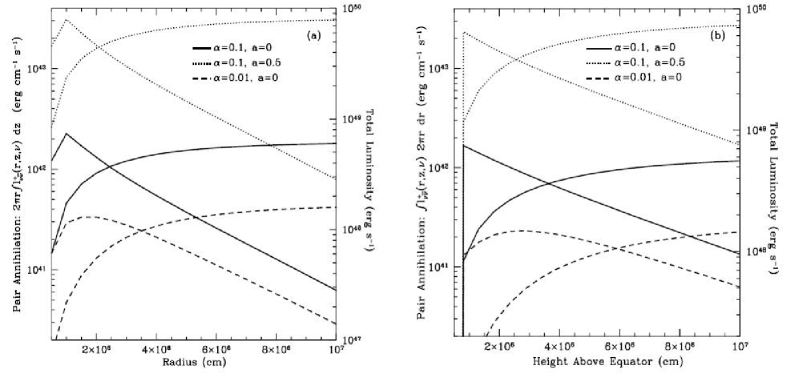
Figure 2.7: $\nu\bar{\nu}$ annihilation luminosity distribution along the disk radius (left panel) and the z-direction (right panel) for $\dot{M}=0.1M_{\odot}$ s^-1 and the mass of BH $M=3.0M_{\odot}$. The total luminosity out to each radius is also plotted (Popham et al. 1999).

$\dot{M}$	$\alpha$	$a$	$M$	$L_{\nu}$	$L_{\nu\bar{\nu}}$	Efficiency
($M_{\odot}$ s-1)			($M_{\odot}$)	(1051 ergs s-1)	(1051 ergs s-1)	%
0.01	0.1	0	3	0.015	$3.9\times 10^{-8}$	0.0003
0.01	0.03	0	3	0.089	$2.9\times 10^{-7}$	0.0003
0.01	0.01	0	3	0.650	$9.0\times 10^{-6}$	0.001
0.01	0.1	0.5	3	0.036	$5.9\times 10^{-7}$	0.002
0.01	0.01	0	10	0.049	$6.4\times 10^{-9}$	$10^{-5}$
0.05	0.1	0.5	3	1.65	$1.8\times 10^{-3}$	0.11
0.1	0.1	0	3	3.35	$3.0\times 10^{-3}$	0.09
0.1	0.1	0	3	6.96	$1.7\times 10^{-3}$	0.02
0.1	0.03	0	3	6.15	$8.0\times 10^{-4}$	0.01
0.1	0.01	0.5	3	8.03	0.039	0.5
0.1	0.1	0.95	3	46.4	2.0	4.2
0.1	0.1	0.95	6	26.2	0.79	3.0
1.0	0.1	0	3	86.3	0.56	0.6
1.0	0.1	0.5	3	142	3.5	2.5
10.0	0.1	0	3	781?	200?	26?
10.0	0.1	0.5	3	1280?	820?	64?

Table 2.2: The neutrino annihilation efficiency for different cases. (Popham, Woosley, & Fryer 1999).

Table 2.2 gives the neutrino annihilation energies and efficiencies for all models studied by Popham et al. (1999). The efficiency increases with the increasing of accretion rate and spin parameter $a$. The energy conversion efficiencies become extremely high for $\dot{M}=10M_{\odot}$ s^-1 . However, the results showed in Table 2.2 is too optimistic, as they do not consider neutrino opacity and overestimate the neutrino luminosity. Di Matteo et al. (2002) showed that the effect of neutrino opacity becomes significant for $\dot{M}>1M_{\odot}$ s^-1, and recalculated the annihilation rate by

$$L_{\nu\bar{\nu}} \sim 6\times 10^{-35}\frac{2\varepsilon_{\nu}L_{\nu}^{2}}{\pi c^{2}[1-(r_{\rm min}/r_{rmsurf})^{2}]^{2}}$$ (2.155)

$$\times\frac{1}{r_{rmsurf}}\int_{0}^{\infty}d\epsilon\Phi(\textrm{cos}\theta_{\rm min}-\textrm{cos}\theta_{\rm surf})^{2}\,\textrm{ergs}\,\textrm{s}^{-1},$$

where $L_{\nu}$ is the neutrino luminosity, $r_{\rm min}$ is the inner edge of the disk, $r_{\rm surf}$ is the radius where $\tau_{\nu}=2/3$, and $\varepsilon_{\nu}$ is the average energy of the escaping neutrinos. Di Matteo et al. (2002) demonstrated that the $L_{\nu\bar{\nu}}$ increases up to its maximum value of $\sim 10^{50}\,\textrm{ergs}\,\textrm{s}^{-1}$ at $\dot{M}>1M_{\odot}$ s^-1 and decreases for large $\dot{M}$. Thus Di Matteo et al. (2002) concluded that the annihilation in hyperaccreting BHs is an inefficient mechanism for liberating large amounts of energy. However, they neglected the neutrino emission from the region with neutrino optical depth $\tau>2/3$. Gu et al. (2006), on the other hand, showed that the energy released by annihilation is still sufficient, if the contribution from the optically thick region of the neutrino-cooled disks $\tau>2/3$ is included. Liu et al. (2007) improved the results of Gu et al. (2007) based on more elaborate calculations similar to Kohri et al. (2005). The electron degeneracy and the lower $Y_{e}<0.5$ resulting from the neutronization processes indeed suppress the neutrino emission considerably, thus the resulting $L_{\nu}$ and $L_{\nu\bar{\nu}}$ are lower than the simplified calculations by Gu et al. (2006). However, the corrected $L_{\nu\bar{\nu}}$ still reaches to $\sim 10^{52}$ ergs s^-1 for $\dot{M}\sim 10M_{\odot}$ s^-1, thus can provide the energy of GRBs. Figure 2.8 gives the neutrino radiation efficiency $\eta_{\nu}(\equiv L_{\nu}/\dot{M}c^{2})$ and neutrino annihilation efficiency $\eta_{\nu\bar{\nu}}(\equiv L_{\nu\bar{\nu}}/L_{\nu}$) as a function of accretion rate. $\eta_{\nu\bar{\nu}}$ increases rapidly with increasing $\dot{M}$. Figure 2.9 is the contour of $2\pi rl_{\nu\bar{\nu}}^{+}$ in units of ergs s^-1 cm^-2. Similar to the results in Popham et al. (1999), the $\nu\bar{\nu}$-annihilation strongly concentrates near the central region of space. Nearly 60% of the total annihilation luminosity is ejected from the region $r<20r_{g}$. Also, Figure 2.9 shows that the annihilation luminosity varies more rapidly along the $z$-direction than along the $r$-direction.

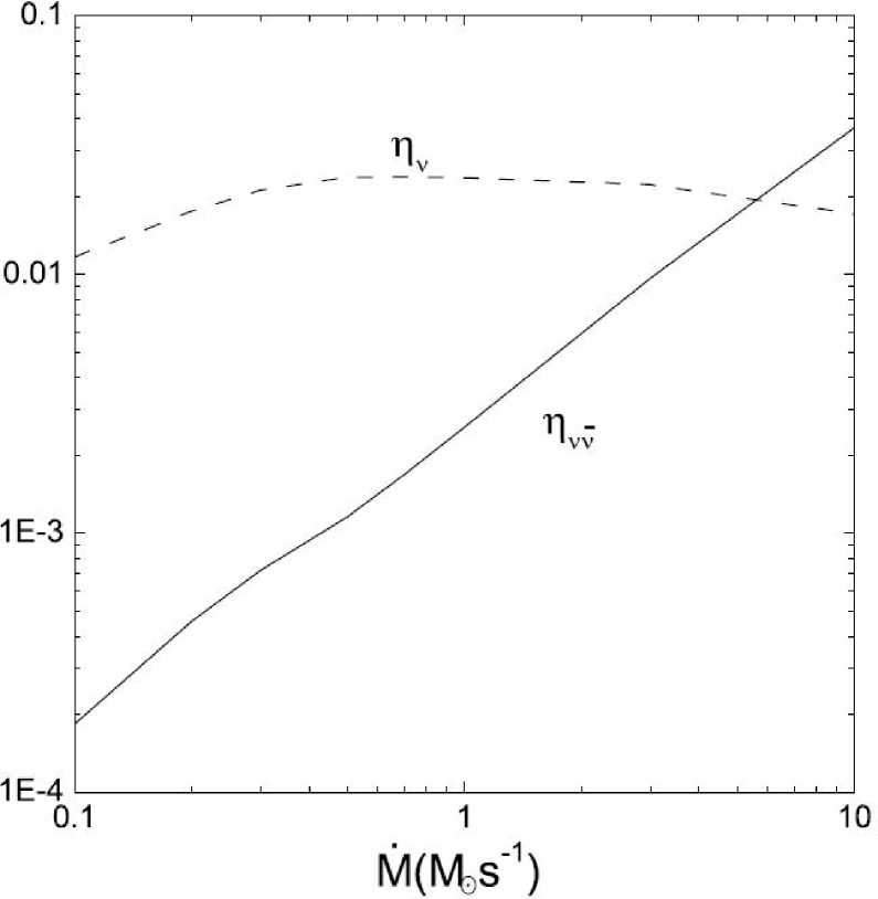
Figure 2.8: Neutrino emission efficiency $\eta_{\nu}$ and neutrino annihilation efficiency $\eta_{\nu\bar{\nu}}$ with $M=3M_{\odot}$, $\alpha=0.1$ (Liu et al. 2007).

Figure 2.9: Contours of the $\nu\bar{\nu}$-annihilation luminosity above the disk in units of ergs s^-1 cm^-2. The parameters are the same as in Fig. 2.8 (Liu et al. 2007).

Although the space distribution of the $\nu\bar{\nu}$-annihilation energy deposition rate can be calculated, it is less clear how could such process produce a narrowly collimated relativistic jet, which is required in the GRB inner shock model. In the collapsar scenario, as mentioned in §1.3.3, Aloy et al. (2000) and Zhang et al. (2003, 2004) showed that the jets from the central BH+disk systems are collimated by their passage through passage through the stellar mantle. But how can a jet, or called “the seed of jet", forms inside $10^{17}$ cm? MacFayden et al. (1999, 2001) discussed that it is not possible to produce a strong jet very early when the momentum of the infalling material along the axis is too high. At $\sim 1$ s, for example, the density of the infalling material is $\geq 10^{7}$ g cm^-3 and its velocity is $\sim 10^{10}$ cm s^-1 for Type I collapsar. Thus any energy deposited by neutrino will be advected into the BH. As time passes, the density especially the density along the polar direction declines, and a disk is formed with the accretion rate up to $\sim 0.1M_{\odot}$ s^-1 about 10 s after core collapse. Thus MacFayden et al. (1999, 2001) discussed that the jets could be initiated when the disk has fully formed, although the initial jets are not well collimated. However, their work did not includes the detailed microphysics of the $\nu\bar{\nu}$-annihilation heating for jets formation. More detailed Mewtonian simulations (e.g., Nagataki et al. 2007) and GR simulations (e.g., Nagataki et al. 2009) showed that, the $\nu\bar{\nu}$-annihilation processes are not efficient to launch a relativistic jet.

Figure 2.10: Density contour with velocity fields for BH-disk model without magnetic fields in Nagataki et al. (2007): $t=2.1s$ (left panel) and $t=2.2s$ (right panel). The central region is $r\leq 10^{8}$ cm in this figure. No jet is launched.

Figure 2.10 shows the density contour of the central region of collapsar without magnetic fields at $t=2.1$ s and $t=2.2$ s. No jet occurs in this case, partly because the accretion rate which drops monotonically from $\sim 0.1M_{\odot}$ s^-1 to $\sim 10^{-3}M_{\odot}$ s^-1 is not high enough to provide energy along the polar axis. It is possible longterm simulations (at least $\sim 10$ s) is needed to see whether the jets could be formed.

Besides the collapsar scenario, jets formation after compact object mergers has also been studied. As the environment outside the BH+disk systems $>10^{7}$ cm does not collimate the initial jets as showed in the stellar mantle of collapsars in this case, other mechanism should be considered. For example, Rosswog et al. (2003) found that the $\nu\bar{\nu}$-annihilation may fail to explain the apparent isotropized energies implied for short GRBs, unless the jet is beamed into less than 1 per cent of the solid angle. They argued that the energetic, neutrino-driven wind may have enough pressure, and thus provide adequate collimation to the $\nu\bar{\nu}$-annihilation-driven jet, based on the mechanism pointed out by Levinson & Eichler (2000) that the pressure and inertia of a baryonic wind can lead to the collimation of a baryon-poor jet, However, such pressure-driven collimation was not self-consistently obtained in the simulations of Rosswog et al. (2003). As a result, it is still an open question that whether the $\nu\bar{\nu}$-annihilation mechanism is efficient to launch a relativistic collimated jet which can produce a GRB.

2.8 MHD Processes and Jet Production

Jets produced in accreting systems surrounded by magnetic fields via MHD processes have been widely studied in various astrophysics objects such as active galactic nuclei, galactic microquasars as well as GRBs. Strong magnetic fields up to $10^{14}-10^{15}$ G is required to launch relativistic Poynting-flux-jets from the stellar-mass BH+ diks systems and rive the GRB phenomena. Even if the initial magnetic fields are low in the progenitors such as weak magnetic massive collapsar, it is still expected that magnetic fields can be amplified by the magneto-rotational instability (MRI, Balbus & Hawley, 1991; or see Balbus & Hawley 1998 for a review). Although the mechanisms for the creation of MHD jets are still a matter of much debate. there are two basic types of MHD mechanisms that may account for the jet formation (Garofalo 2009). The first involves a magnetocentrifugal or MHD wind similiar to the solar wind phenomena (e.g., Blandford & Payne 1982; Koide et al. 1998, 1999). The second class of mechanism applied only to BH accretors, which drive jets by their ergosphere (e.g., Pernose 1969; Blandford & Znajek 1977).

Blandford & Payne (1982) illustrated that a centrifugally driven wind from the disk is possible if the poloidal component of the magnetic field makes an angle of less than $\sim 60^{\circ}$ with the disk surface. At large distances from the disk, the toroidal component of the field becomes important and collimates the outflow into a pair of anti-parallel jets moving perpendicular to the disk. Close to the disk, the flow is probably driven by gas pressure in a hot magnetically dominated corona. As a result, magnetic stresses can extract the angular momentum from a thin disk and enable matter to be acreted, independently of the disk viscosity. Although the basic purpose of Blandford & Payne (1982) was to explain the radio jets which emerging from the AGNs, this mechanism does also work in the stellar-mass BH+ disk system as the GRB central engine. However, this mechanism tends to produce relatively cold jets, in the sense that the thermal energy of the jet is not initially large compared to either the rest mass of the jet or the jet kinetic energy. MacFadyen et al. (2001) discussed that cold MHD jets may be collimated both by magnetic fields and by geometry.

Christodolou (1970) first discussed that for a rotating hole described by the Kerr metric, a portion of the rest mass can be regarded as “reducible" in the snes that it can be removed and extracted to infinity. The possibility of extracting the reducible mass was discussed by Pernose (1969) that the existence of negative energy orbits within the ergosphere surrounding a Kerr BH permits the mechanical extraction of energy via certain types of particle collision (see Teukolsky & Press 1974 for a similar process study). However, neither process seems likely to operate effectively in any astrophysical situation. Blandford & Znajek (1977) studied a rotating BH surrounded by a stationary axisymmetric magnetized plasma (see Figure 2.11).

Figure 2.11: Schematic cross-section of BH and magnetosphere. A current $I$ is flowing from the magnetosphere into the hole, and back out of the hole into the disk D lying in the $\theta=\pi/2$ plane. Between the disk and the hole there is a transition region $T$ in which the matter is falling from the disk to the hole. More details can be seen in Blandford & Znajek (1977).

They showed an effective mechanism which can extracted the rotational energy of the BH by ergosphere. This mechanism appears when the charges around the BH are sufficient to provide the force-free condition. The fundamental equations describing a stationary axiymmetric magnetosphere were derived in Blandford & Znajek (1977), and the details of the energy and angular momentum balance were discussed. The poloidal components of the conserved electromagnetic energy flux $\mathscr{E}_{r}$ and angular momentum flux $\mathscr{L}_{r}$ satisfy

$$\mathscr{E}_{r}=\omega(\Omega_{H}-\omega)\left(\frac{A_{\phi,\theta}}{r_{+}^{2}+a^{2}cos^{2}\theta}\right)(r_{+}^{2}+a^{2})\epsilon_{0},$$ (2.156)

$$\mathscr{L}_{r}=\mathscr{E}_{r}/\omega,$$ (2.157)

where $\Omega_{H}\equiv a/(r_{+}^{2}+a^{2})$ is the angular velocity of the hole with $r_{+}$ being the radius of the event horizon, $\omega$ is the “rotation frequency" of the electromagnetic fields, and $A_{\phi}$ is the $\phi$-component of a vector potential $A_{\mu}$. Here the Boyer-Lindqust coordinates are adopted. Thus $\mathscr{E}_{r},\mathscr{L}_{r}\geq 0$ implies $0\leq\omega\leq\Omega_{H}$. Furthermore, Blandford & Znajek (1977) adopted a perturbation technique to provide approximate solutions for slowly rotating holes $a\ll 1$. Particularly, for the force-free magnetosphere with a paraboloidal magnetic force, the extracted energy appears to be focused along the rotation axis, and the power radiated satisfies

$$L_{BZ}\approx\frac{1}{32}\frac{\omega(\Omega_{H}-\omega)}{\Omega_{H}^{2}}B^{2}r_{+}^{2}a^{2}c.$$ (2.158)

Although the formula (2.158) was originally obtained for $a\ll 1$, Komissarov (2001) has performed a numerical study of the BZ solution concluding that the formula is valid at least up to $a=0.9$.

GRMHD simulations in the Kerr metric in 2D (McKinney & Gammie 2004; Mckiney 2005, 2006; Garofalo 2009) and in 3D (De Villiers et al. 2003, 2005; Hirose et al. 2004; Krolik et al. 2005; Hawley & Krolik 2006) have been carried out to investigate the properties of the MHD jets from the central BHs surrounded by the magnetized plasma. For example, McKinney & Gammie (2004) used a general relativistic MHD code (HARM) to evolve a weakly magnetized thick disk around a Kerr BH. They found an outward electromagnetic energy flux on the event horizon as anticipated by Blandford & Znajek (1977). The funnel region near the polar axis of the BH is consistent with the BZ model. The outward electromagnetic energy flux is, however, overwhelmed by the inward flux of energy associated with the rest-mass and internal energy of the accreting plasma. This result that suggested confirms work by Ghosh & Abramowicz (1997) that suggested the BZ luminosity should be small or comparable to the nominal accretion luminosity. Hawley & Krolik (2006) examined the unbound axial outflows (jets) that develop within 3D GRMHD simulations. Different to most of other studies that magnetic field boundary conditions are imposed on the simulations, they simulated how accretion dynamics self-consistently creates magnetic field and explore the outflows and jets. They jets have two major components: a matter-dominated outflow that moves at a modest velocity ($v/c\sim 0.3$) along the centrifugal barrier surrounding an evacuated axial funnel, and a highly relativistic Poynting flux-dominated jet within the funnel. The funnel-wall jet is accelerated and collimated by magnetic and gas pressure forces in the inner torus and the surrounding corona.

Figure 2.12: Specific angular momentum and mass flux at late time in the KDPs simulation in Hawley & Krolik (2006), Colar contours show the mass-weighted mean angular momentum in the funnel-wall outflow. Th radius is in unit of $M$ with $G=c=1$.

The Poynting flux jet results from the formation of a large-scale radial magnetic field within the funnel. This field is spun by the rotating spacetime of the BH. Figure 2.12 shows the specific angular momentum and mass flux at late time of MHD outflows and jets evolution in Hawley & Krolik (2006). Their results are in general agreement with those of Blandford & Znajek (1977), but there are also specific differences from the classical Blandford-Znajek model. For instance, it is not in general in a state of force-free equilibrium in the magnetically dominated funnel region. Also, the electromangetic luminosity in the outflows that places entirely as a by-produce of accretion in Hawley & Krolik (2006), whereas in the classical BZ model there was zero accretion. Recently, Garofalo (2009) studies the spin-dependence of the BZ effect. Large scale magnetic fields are enhanced on the BH compared to the inner accretion flow and that the ease with which this occurs for lower prograde BH spin, produces a spin dependence in the BZ effect.

The GRMHD simulations mentioned above are not directly applicable to the GRB case, as they do not consider the dense disks with huge accretion rate with a fraction of solar mass per second and the neutrino cooling and heating processes. Nagataki (2009) studied the outgoing Poynting flux exists at the horizon of the central BH around the polar region inside a collapsar. They concluded that the jet is launched mainly by the magnetic field amplified by the gravitational collapse and differential rotation around the BH, rather than the BZ mechanism in this study. However, no microphysics is included in the code such as nuclear reactions, neutrino processes, and equation of state for dense matter. Further studied should be done in subsequent work.

Chapter 3 Hyperaccretion Disks around Neutron Stars

3.1 Introduction

Gamma-ray bursts (GRBs) are commonly divided into two classes: short-duration, hard-spectrum bursts, and long-duration, soft-spectrum bursts. The observations have provided growing evidence that short bursts result from the mergers of compact star binaries and long bursts originate from the collapses of massive stars (for recent reviews see Zhang & Mészáros 2004; Piran 2004; Mészáros 2006; Nakar 2007). It is usually assumed that both a compact-star merger and a massive-star collapse give rise to a central black hole and a debris torus around it. The torus has a mass of about $0.01-1M_{\odot}$ and a large angular momentum enough to produce a transient accretion disk with a huge accretion rate up to $\sim 1.0M_{\odot}\,{\rm s}^{-1}$. The accretion timescale is short, e.g., a fraction of one second after the merger of two neutron stars, and tens of seconds if a disk forms due to fallback of matter during the collapse process.

The hyperaccretion disk around a black hole is extremely hot and dense. The optical depth of the accreting gas is so enormous that radiation is trapped inside the disk and can only be advected inward. However, in some cases, this hot and dense disk can be cooled via neutrino emission (Narayan et al. 1992). According to the disk structure and different cooling mechanisms, flows in the disk fall into three types: advection-dominated accretion flows (ADAFs), convection-dominated accretion flows (CDAFs), and neutrino-dominated accretion flows (NDAFs). The first two types of flow are radioactively inefficient (Narayan et al. 1998, 2000, 2001) and the final type cools the disk efficiently via neutrino emission (Popham et al. 1999; Di Matteo et al. 2002). In view of effects of these three flows, hyperaccretion disks around black holes have been studied both analytically and numerically (e.g., see Popham et al. 1999; Narayan et al. 2001; Kohri & Mineshige 2002; Di Matteo et al. 2002; Gu et al. 2006; Chen & Beloborodov 2007; Liu et al. 2007; Janiuk et al. 2007).

However, newborn neutron stars have been invoked to be central engines of GRBs in some origin/afterglow models. First, the discovery of X-ray flares by Swift implies that the central engines of some GRBs are in a long-living activity (at least hundreds of seconds) after the bursts (Zhang 2007). This provides a challenge to conventional hyperaccretion disk models of black holes. Recently, Dai et al. (2006) argued that newborn central compact objects in the GRBs could be young neutron stars, at least transiently-existing neutron stars, rather than black holes (for alternative models see Perna et al. 2006 and Proga & Zhang 2006). These neutron stars may have high angular momentum and their maximum mass may be close to or slightly larger than the upper mass limit of nonrotating Tolman-Oppenheimer-Volkoff neutron stars. According to this argument, Dai et al. (2006) explained X-ray flares of short GRBs as being due to magnetic reconnection-driven events from highly-magnetized millisecond pulsars. It is thus reasonable to assume a unified scenario: a prompt burst originates from a highly-magnetized, millisecond-period neutron star surrounded by a transient hyperaccretion disk, and subsequent X-ray flares are due to a series of magnetic activities of the neutron star.

Second, the shallow decay phase of X-ray afterglows about several hundreds of seconds after a sizable fraction of GRBs discovered by Swift has been understood as arising from long-lasting energy injection to relativistic forward shocks (Zhang 2007). It was proposed before Swift observations that pulsars in the unified scenario mentioned above can provide energy injection to a forward shock through magnetic dipole radiation, leading to flattening of an afterglow light curve (Dai & Lu 1998a; Zhang & Mészáros 2001; Dai 2004). Recent model fitting (Fan & Xu 2006; Yu & Dai 2007) and data analysis (Liang et al. 2007) indeed confirm this result. An ultra-relativistic pulsar wind could be dominated by electron/positron pairs and its interaction with a postburst fireball gives rise to a reverse shock and forward shock (Dai 2004). The high-energy emission due to inverse-Compton scattering in these shocks is significant enough to be detectable with the upcoming Gamma-ray Large-Area Space Telescope (Yu et al. 2007).

Third, we note that, in some origin models of GRBs (e.g., Kluźniak & Ruderman 1998; Dai & Lu 1998b; Wheeler et al. 2000; Wang et al. 2000; Paczyński & Haensel 2005), highly-magnetized neutron stars or strange quark stars surrounded by hyperaccretion disks resulting from fallback of matter could occur during the collapses of massive stars or the mergers of two neutron stars. A similar neutron star was recently invoked in numerical simulations of Mazzali et al. (2006) and data analysis of Soderberg et al. (2006) to understand the properties of supernova SN 2006aj associated with GRB 060218. In addition, hyperaccretion disks could also occur in type-II supernovae if fall-back matter has angular momentum. It would be expected that such disks play an important role in supernova explosions via neutrino emission, similar to some effects reviewed by Bethe (1990).

Based on these motivations, we here investigate a hyperaccretion disk around a neutron star. To our knowledge, this paper is the first to study hyperaccretion disks around neutron stars related possibly with GRBs. Chevalier (1996) discussed the structure of dense and neutrino-cooled disks around neutron stars. He considered neutrino cooling due to electron-positron pair annihilation, which is actually much less important than the cooling due to electron-positron pair capture in the hyperaccreting case of our interest, since the accretion rate assumed in Chevalier (1996) ($\sim M_{\odot}\,{\rm yr}^{-1}$) is much less than that of our concern ($\sim 0.1M_{\odot}\,{\rm s}^{-1}$). In this chapter we consider several types of neutrino cooling by using elaborate formulae developed in recent years. In addition, we focus on some differences between black hole and neutron star hyperaccretion. A main difference is that, the internal energy in an accretion flow may be advected inward into the event horizon without any energy release if the central object is a black hole, but the internal energy must be eventually released from the disk if the central object is a neutron star, because the stellar surface prevents any heat energy from being advected inward into the star. Since the accretion rate is always very high, the effective cooling mechanism in the disk is still neutrino emission, and as a result, the efficiency of neutrino cooling of the entire disk around a neutron star should be higher than that of a black hole disk.

There have been a lot of works to study accretion onto neutron stars in binary systems (e.g., Shapiro & Salpeter 1975; Kluźniak & Wilson 1991; Medvedev & Narayan 2001; Frank et al. 2002) and supernova explosions (e.g., Chevalier 1989, 1996; Brown & Weingartner 1994; Kohri et al. 2005). In the supernova case, spherically symmetric accretion onto neutron stars (the so-called Bondi accretion) was investigated in detail. In particular, Kohri et al. (2005) tried to use the hyperaccretion disk model with an outflow wind to explain supernova explosions. In the binary systems, as the accretion rate is not larger than the Eddington accretion rate ($\sim 10^{-8}M_{\odot}\,{\rm yr}^{-1}$), the physical properties of the disk must be very different from those of a hyperaccretion disk discussed here.

This chapter is organized as follows: in §3.3.2, we describe a scheme of our study of the structure of a quasi-steady disk. We propose that the disk around a neutron star can be divided into two regions: inner and outer disks. Table 3.1 gives the notation and definition of some quantities in this chapter. In order to give clear physical properties, we first adopt a simple model in §3.3, and give both analytical and numerical results of the disk properties. In §3.4, we study the disk using a state-of-the-art model with lots of elaborate considerations about the thermodynamics and microphysics, and compare results from this elaborate model with those from the simple model. §3.5 presents conclusions and discussions.

notation	definition	§/Eq.
$m$	mass of the central neutron star, $m=M/1.4M_{\odot}$	§3.3.1, (3.21)
$\dot{m}_{d}$	mass accretion rate, $\dot{m}_{d}=\dot{M}/0.01M_{\odot}\,{\rm s}^{-1}$	§3.3.1, (3.21)
$Y_{e}$	ratio of the electron to nucleon number density in the disk	§3.2.2, (3.9)
$r_{*}$	radius of the neutron star	§3.2.3, (3.13)
$r_{\rm out}$	outer radius of the disk	§3.2.3, (3.13)
$\Omega_{*}$	angular velocity of the stellar surface	§3.3.3, (3.52)
$\varepsilon$	efficiency of energy release in the inner disk	§3.2.3, (3.17)
$\tilde{r}$	radius between the inner and outer disks	§3.2.3, (3.12)
$\bar{r}$	radius between the neutrino optically-thick & -thin regions	§3.3.2, (3.50)
$k=\bar{r}/\tilde{r}$	parameter to measure the neutrino optically-thick region	—
$f=1-\sqrt{\frac{r_{*}}{r}}$	useful factor as a function of $r$	§3.2.2, (3.7)
$\tilde{f}=1-\sqrt{\frac{r_{*}}{\tilde{r}}}$	value of $f$ at radius $\tilde{r}$	§3.3.2, (3.41)
$\bar{f}_{\nu}$	average efficiency of neutrino cooling in the outer disk	§3.2.3, (3.13)

Table 3.1: Notation and definition of some quantities in this chapter.

3.2 Description of Our Study Scheme

3.2.1 Motivations of a two-region disk

We study the quasi-steady structure of an accretion disk around a neutron star with a weak outflow. We take an accretion rate to be a parameter. For the accretion rates of interest to us, the disk flow may be an ADAF or NDAF. In this chapter, we do not consider a CDAF. Different from the disk around a black hole, the disk around a neutron star should eventually release the gravitational binding energy of accreted matter (which is converted to the internal energy of the disk and the rotational kinetic energy) more efficiently.

The energy equation of the disk is (Frank et al. 2002)

$$\Sigma v_{r}T\frac{ds}{dr}=Q^{+}-Q^{-},$$ (3.1)

where $\Sigma$ is the surface density of the disk, $v_{r}$ is the radial velocity, $T$ is the temperature, $s$ is the entropy per unit mass, $r$ is the radius of a certain position in the disk, and $Q^{+}$ and $Q^{-}$ are the energy input (heating) and the energy loss (cooling) rate in the disk. From the point of view of evolution, the structure of a hyperaccretion disk around a neutron star should be initially similar to that of the disk around a black hole, because the energy input is mainly due to the local viscous dissipation, i.e., $Q^{+}=Q^{+}_{\rm vis}$. However, since the stellar surface prevents the matter and heat energy in the disk from advection inward any more, a region near the compact object should be extremely dense and hot as accretion proceeds. Besides the local viscous heating, this inner region can also be heated by the energy ($Q^{+}_{\rm adv}$) advected from the outer region of the disk. Thus, the heat energy in this region may include both the energy generated by itself and the energy advected from the outer region, that is, we can write $Q^{+}=Q^{+}_{\rm vis}+Q^{+}_{\rm adv}$. Initially, such a region is so small (i.e., very near the compact star surface) that it cannot be cooled efficiently for a huge accretion rate ($\sim 0.01-1M_{\odot}\,{\rm s}^{-1}$). As a result, it has to expand its size until an energy balance between heating and cooling is built in this inner region. Such an energy balance can be expressed by $Q^{+}=Q^{-}$ in the inner region of the disk.

Once this energy balance is built, the disk is in a steady state as long as the accretion rate is not significantly changed. For such a steady disk, therefore, the structure of the outer region is still similar to that of the disk around a black hole, but the inner region has to be hotter and denser than the disk around a black hole, and could have a different structure from both its initial structure and the outer region that is not affected by the neutron star surface.

Based on the above consideration, the hyperaccretion disk around a neutron star could have two different regions. In order to discuss their structure using a mathematical method clearly, as a reasonable approximation, we here divide the steady accretion disk into an inner region and an outer region, called inner and outer disks respectively. The outer disk is similar to that of a black hole. The inner disk, depending on its heating and cooling mechanisms discussed above, should satisfy the entropy conservation condition $Tds/dr\propto Q^{+}-Q^{-}=0$, and thus we obtain $P\propto\rho^{\gamma}$, where $P$ and $\rho$ are the pressure and the density of the disk, and $\gamma$ is the adiabatic index of the disk gas. Also, the radial momentum equation is

$$(\Omega^{2}-\Omega_{K}^{2})r-\frac{1}{\rho}\frac{d}{dr}(\rho c_{s}^{2})=0,$$ (3.2)

where $\Omega$ and $\Omega_{K}$ are the angular velocity and Keplerian angular velocity of the inner disk, and $c_{s}=\sqrt{P/\rho}$ is the isothermal sound speed. We here neglect the radial velocity term $v_{r}dv_{r}/dr$ since we consider the situation $v_{r}dv_{r}/dr\ll|\Omega^{2}-\Omega_{K}^{2}|r$, which can still be satisfied when $v_{r}\ll r\Omega_{K}$ with $\Omega\sim\Omega_{K}$ but $|\Omega-\Omega_{K}|\geq v_{r}/r$. Equation (3.2) gives $\Omega\propto r^{-3/2}$ and $c_{s}\propto r^{-1/2}$. Moreover, from the continuity equation, we have $v_{r}\propto(\rho rH)^{-1}$ with the disk’s half-thickness $H=c_{s}/\Omega\propto r$. Thus we can derive a self-similar structure in the inner region of the hyperaccretion disk of a neutron star,

$$\rho\propto r^{-1/(\gamma-1)},\,\,P\propto r^{-\gamma/(\gamma-1)},\,\,v_{r}\propto r^{(3-2\gamma)/(\gamma-1)},$$ (3.3)

This self-similar structure has been given by Chevalier (1989) and Brown & Weingartner (1994) for Bondi accretion under the adiabatic condition and by Medvedev & Narayan (2001) and Medvedev (2004) for disk accretion under the entropy conservation condition. In addition, if the gas pressure is dominated in the disk, we have $\gamma=5/3$ so that equation (3.3) becomes $\rho\propto r^{-3/2}$, $P\propto r^{-5/2}$, and $v_{r}\propto r^{-1/2}$, which have been discussed by Spruit et al. (1987) and Narayan & Yi (1994).

An important problem we next solve is to determine the size of the inner disk. Since the total luminosity of neutrinos emitted from the whole disk significantly varies with the inner-region size, we can estimate the inner region size by solving an energy balance between neutrino cooling and heating in the entire disk. The details will be discussed in §3.2.3.

Finally, we focus on two problems in this subsection. First, we have to discuss a physical condition of the boundary layer between the outer and inner disks. There are two possible boundary conditions. One condition is to assume that a stalled shock exists at the boundary layer. Under this assumption, the inner disk is a post-shock region, and its pressure, temperature and density just behind the shock are much higher than those of the outer disk in front of the shock. The other condition is to assume that no shock exists in the disk, and that all the physical variables of two sides of this boundary change continuously. We now have to discuss which condition is reasonable.

Let us assume the mass density, pressure, radial velocity, and internal energy density of the outer disk along the boundary layer to be $\rho_{1}$, $P_{1}$, $v_{1}$, and $u_{1}$, and the corresponding physical variables of the inner disk to be $\rho_{2}$, $P_{2}$, $v_{2}$, and $u_{2}$ at the same radius. Thus the conservation equations are

$$\begin{array}[]{ll}\rho_{1}v_{1}=\rho_{2}v_{2}\\ P_{1}+\rho_{1}v_{1}^{2}=P_{2}+\rho_{2}v_{2}^{2}\\ (u_{1}+P_{1}+\rho_{1}v_{1}^{2}/2)/\rho_{1}=(u_{2}+P_{2}+\rho_{2}v_{2}^{2}/2)/\rho_{2}.\end{array}$$ (3.4)

From the Rankine-Hugoniot relations, we know that if $P_{2}\gg P_{1}$, the densities of two sides of the boundary layer are discontinuous, which means that a strong shock exists between the inner and outer disks. On the other hand, if $P_{1}\sim P_{2}$, we can obtain $\rho_{1}\sim\rho_{2}$, which means that only a very weak shock forms at this boundary layer, or we can say that no shock exists. Therefore, we compare $P_{1}$ and $\rho_{1}v_{1}^{2}$ of the outer disk. If $P_{1}\ll\rho_{1}v_{1}^{2}$ or $c_{s}\ll v_{1}$, we can assume that a stalled shock exists at the boundary layer, i.e., the first boundary condition is correct. If $P_{1}\gg\rho_{1}v_{1}^{2}$ or $c_{s}\gg v_{1}$, otherwise, we consider $P_{1}\sim P_{2}$, and thus no shock exists. In §3.3 and §3.4, we will use this method to discuss which boundary condition is reasonable.

Second, what we want to point out is that the effect of the magnetic field of the central neutron star is not considered in this chapter. We estimate the order of magnitude of the Alfvén radius by using the following expression (Frank et al 2002), $r_{A}\simeq 2.07\times 10^{4}\dot{m}_{d}^{-2/7}m^{-1/7}\mu_{30}^{4/7}$, where $\dot{m}_{d}=\dot{M}/0.01M_{\odot}\,{\rm s}^{-1}$ is the accretion rate, $m=M/1.4M_{\odot}$ is the mass of the neutron star, and $\mu_{30}$ is the magnetic moment of the neutron star in units of $10^{30}{\rm G}\,{\rm cm}^{3}$. Let $r_{*}$ be the neutron star radius. If the stellar surface magnetic field $B_{s}\leq B_{s,{\rm cr}}=2.80\times 10^{22}\dot{m}_{d}^{1/2}m^{1/4}r_{*}^{-5/4}\,$G or $B_{s}\leq B_{s,{\rm cr}}=0.89\times 10^{15}\dot{m}_{d}^{1/2}m^{1/4}\,$G when $r_{*}=10^{6}$ cm, then the Alfvén radius $r_{A}$ is smaller than $r_{*}$. The critical value $B_{s,{\rm cr}}$ increases with increasing the accretion rate. This implies that the stellar surface magnetic field affects the structure of the disk significantly if $B_{s}\geq B_{s,{\rm cr}}\sim 10^{15}-10^{16}\,$G for typical accretion rates. Therefore, we assume a neutron star with surface magnetic field weaker than $B_{s,{\rm cr}}$ in this chapter. This assumption is consistent with some GRB-origin models such as Kluźniak & Ruderman (1998), Dai & Lu (1998b), Wang et al. (2000), Paczyński & Haensel (2005), and Dai et al. (2006), because these models require a neutron star or strange quark star with surface magnetic field much weaker than $B_{s,{\rm cr}}$.

3.2.2 Structure of the outer disk

Here we discuss the structure of the outer disk based on the Newtonian dynamics and the standard $\alpha$-viscosity disk model for simplicity. The structure of the hyperaccretion disk around a stellar-mass black hole has been discussed in many previous works. The method and equations we use here are similar to those in the previous works since the outer disk is very similar to the disk around a black hole.

We approximately consider the angular velocity of the outer disk to be the Keplerian value $\Omega_{K}=\sqrt{GM/r^{3}}$. The velocity $\Omega_{K}$ should be modified in a relativistic model of accretion disks (Popham et al. 1999; Chen & Beloborodov 2007), but we do not consider it in this chapter. We can write four equations to describe the outer disk, i.e., the continuity equation, the energy equation, the angular momentum equation and the equation of state.

The continuity equation is

$$\dot{M}=4\pi r\rho v_{r}H\equiv 2\pi r\Sigma v_{r},$$ (3.5)

where the notations of the physical quantities have been introduced in $\S$3.2.1.

In the outer disk, the heat energy could be advected inward and we take $Q_{\rm adv}^{-}=(1/2)\Sigma Tv_{r}ds/dr$ to be the quantity of the energy advection rate, where the factor $1/2$ is added because we only study the vertically-integrated disk over a half-thickness $H$. Thus the energy-conservation equation (3.1) is rewritten as

$$Q^{+}=Q_{\rm rad}^{-}+Q_{\rm adv}^{-}+Q_{\nu}^{-}.$$ (3.6)

The quantity $Q^{+}$ in equation (3.6) is the viscous heat energy generation rate per unit surface area. According to the standard viscosity disk model, we have

$$Q^{+}=\frac{3GM\dot{M}}{8\pi r^{3}}f$$ (3.7)

where $f=1-(r_{*}/r)^{1/2}$ (Frank et al. 2002).

The quantity $Q_{\rm rad}^{-}$ in equation (3.6) is the photon cooling rate per unit surface area of the disk. Since the disk is extremely dense and hot, the optical depth of photons is always very large and thus we can take $Q_{\rm rad}^{-}=0$ as a good approximation.

The entropy per unit mass of the disk is (similar to Kohri & Mineshige 2002)

$$s=s_{\rm gas}+s_{\rm rad}=\frac{S_{\rm gas}}{\rho}+\frac{S_{\rm rad}}{\rho}=\sum_{i}n_{i}\left\{\frac{5}{2}\frac{k_{B}}{\rho}+\frac{k_{B}}{\rho}\textrm{ln}\left[\frac{(2\pi k_{B}T)^{3/2}}{h^{3}n_{i}}\right]\right\}+S_{0}+\frac{2}{3}g_{*}\frac{aT^{3}}{\rho},$$ (3.8)

where the summation runs over nucleons and electrons, $k_{B}$ is the Boltzmann constant, $h$ is the Planck constant, $a$ is the radiation constant, $S_{0}$ is the integration constant of the gas entropy, and the term $2g_{*}aT^{3}/3\rho$ is the entropy density of the radiation with $g_{*}=2$ for photons and $g_{*}=11/2$ for a plasma of photons and relativistic $e^{+}e^{-}$ pairs. We assume that electrons and nucleons have the same temperature. Then we use equation (3.8) to calculate $ds/dr$ and approximately take $dT/dr\approx T/r$ and $d\rho/dr\approx\rho/r$ to obtain the energy advection rate,

$$Q_{\rm adv}^{-}=v_{r}T\frac{\Sigma}{2r}\left[\frac{R}{2}\left(1+Y_{e}\right)+\frac{4}{3}g_{*}\frac{aT^{3}}{\rho}\right],$$ (3.9)

where the gas constant $R=8.315\times 10^{7}$ ergs mole^-1 K^-1 and $Y_{e}$ is the ratio of electron to nucleon number density. The first term in the right-hand bracket of equation (3.9) comes from the contribution of the gas entropy and the second term from the contribution of radiation.

The quantity $Q_{\nu}^{-}$ in equation (3.6) is the neutrino cooling rate per unit area. The expression of $Q_{\nu}^{-}$ will be discussed in detail in $\S$3.3 and $\S$3.4.

In this chapter we ignore the cooling term of photodisintegration $Q_{\rm photodis}^{-}$, and approximately take the free nucleon fraction $X_{\rm nuc}\approx 1$. For the disks formed by the collapses of massive stars, the photodisintegration process that breaks down $\alpha$-particles into neutrons and protons is important in a disk region at very large radius $r$. However, the effect of photodisintegration becomes less significant for a region at small radius, where contains less $\alpha$-particles. On the other hand, for the disks formed by the mergers of double compact stars, there will be rare $\alpha$-particles in the entire disk. As a result, we reasonably take all the nucleons to be free ($X_{\rm nuc}\approx 1$) and neglect the photodisintegration process, since we mainly focus on small disks or small regions of the disks (as we will mention in §3.3.4 with the outer boundary $r_{\rm out}$ to be 150 km.)

Furthermore, the angular momentum conservation and the equation of sate can be written as

$$\nu\Sigma=\frac{\dot{M}}{3\pi}f,$$ (3.10)

$$P=P_{e}+P_{\rm nuc}+P_{\rm rad}+P_{\nu},$$ (3.11)

where $\nu=\alpha c_{s}H$ in equation (3.10) is the kinematic viscosity and $\alpha$ is the classical viscosity parameter, and $P_{e}$, $P_{\rm nuc}$, $P_{\rm rad}$ and $P_{\nu}$ in equation (3.11) are the pressures of electrons, nucleons, radiation and neutrinos. In $\S$3.3 we will consider the pressure of electrons in extreme cases and in $\S$3.4 we will calculate the $e^{\pm}$ pressure using the exact Fermi-Dirac distribution function and the condition of $\beta$-equilibrium.

Equations (3.5), (3.6), (3.10) and (3.11) are the basic equations to solve the structure of the outer disk, which is important for us to study the inner disk.

3.2.3 Self-similar structure of the inner disk

In §3.2.1 we introduced a self-similar structure of the inner disk, and described the method to determine the size of the inner disk. Now we will establish the energy conservation equation in the inner disk. We assume that $\tilde{r}$ is the radius of the boundary layer between the inner and outer disks, and that $\tilde{\rho}$, $\tilde{P}$, and $\tilde{v}_{r}$ are the density, pressure and radial velocity of the inner disk just at the boundary layer respectively. From equation (3.3), thus, the variables in the inner disk at any given radius $r$ can be written by

$$\rho=\tilde{\rho}(\tilde{r}/r)^{1/(\gamma-1)},P=\tilde{P}(\tilde{r}/r)^{\gamma/(\gamma-1)},v_{r}=\tilde{v}_{r}(\tilde{r}/r)^{(2\gamma-3)/(\gamma-1)}.$$ (3.12)

We take the outer radius of the accretion disk to be $r_{\rm out}$. The total energy per unit time that the outer disk advects into the inner disk is (Frank et al. 2002)

$$\dot{E}_{\rm adv}=(1-\bar{f}_{\nu})\frac{3GM\dot{M}}{4}\left\{{\frac{1}{\tilde{r}}\left[1-\frac{2}{3}\left(\frac{r_{*}}{\tilde{r}}\right)^{1/2}\right]-\frac{1}{r_{\rm out}}\left[1-\frac{2}{3}\left(\frac{r_{*}}{r_{\rm out}}\right)^{1/2}\right]}\right\},$$ (3.13)

where $\bar{f}_{\nu}$ is the average neutrino cooling efficiency of the outer disk,

$$\bar{f}_{\nu}=\frac{\int_{\tilde{r}}^{r_{\rm out}}Q_{\nu}^{-}2\pi rdr}{\int_{\tilde{r}}^{r_{\rm out}}Q^{+}2\pi rdr}.$$ (3.14)

If the outer disk flow is mainly an ADAF, $Q_{\nu}^{-}\ll Q^{+}$, then $\bar{f}_{\nu}\sim 0$; if the outer disk flow is mainly an NDAF, $Q_{\nu}^{-}\gg Q_{\rm rad}^{-}$ and $Q_{\nu}^{-}\gg Q_{\rm adv}^{-}$, we have $\bar{f}_{\nu}\sim 1$. The heat energy in the inner disk should be released more efficiently than the outer disk, we can still approximately take $\Omega\simeq\Omega_{K}$ in the inner disk, and the maximum power that the inner disk can release is

$$L_{\nu,max} \approx \frac{3GM\dot{M}}{4}\left\{\frac{1}{3r_{*}}-\frac{1}{r_{\rm out}}\left[1-\frac{2}{3}\left(\frac{r_{*}}{r_{\rm out}}\right)^{1/2}\right]\right\}$$ (3.15)

$$-\bar{f}_{\nu}\frac{3GM\dot{M}}{4}\left\{\frac{1}{\tilde{r}}\left[1-\frac{2}{3}\left(\frac{r_{*}}{\tilde{r}}\right)^{1/2}\right]-\frac{1}{r_{\rm out}}\left[1-\frac{2}{3}\left(\frac{r_{*}}{r_{\rm out}}\right)^{1/2}\right]\right\},$$

where we have integrated vertically over the half-thickness. The first term in the right-hand of this equation is the total heat energy per unit time of the entire disk, and the second term is the power taken away through neutrino cooling in the outer disk. Considering $r_{\rm out}\gg r_{*}$, we have

$$L_{\nu,max}\approx\frac{3GM\dot{M}}{4}\left\{\frac{1}{3r_{*}}-\frac{\bar{f}_{\nu}}{\tilde{r}}\left[1-\frac{2}{3}\left(\frac{r_{*}}{\tilde{r}}\right)^{1/2}\right]\right\}.$$ (3.16)

The maximum energy release rate of the inner disk is $GM\dot{M}/4r_{*}$ if the outer disk flow is mainly an ADAF and $\bar{f}_{\nu}\sim 0$. This value is just one half of the gravitational binding energy and satisfies the Virial theorem. If the outer disk flow is an NDAF, then the energy release of the inner disk mainly results from the heat energy generated by its own.

Following the above consideration, most of the energy generated in the disk around a neutron star is still released from the disk, so we have an energy-conservation equation,

$$\int_{r_{*}}^{\tilde{r}}Q_{\nu}^{-}2\pi rdr=\varepsilon\frac{3GM\dot{M}}{4}\left\{{\frac{1}{3r_{*}}-\frac{\bar{f}_{\nu}}{\tilde{r}}\left[1-\frac{2}{3}\left(\frac{r_{*}}{\tilde{r}}\right)^{1/2}\right]}\right\},$$ (3.17)

where $\varepsilon$ is a parameter that measures the efficiency of the energy release. If the central compact object is a black hole, we have $\varepsilon\approx 0$ and the inner disk cannot exist. If the central compact object is a neutron star, we can take $\varepsilon\approx 1$ and thus we are able to use equation (3.17) to determine the size of the inner disk.

3.3 A Simple Model of the Disk

In $\S$3.2, we gave the equations of describing the structure of a hyperaccretion disk. However, additional equations about microphysics in the disk are needed. In order to see the physical properties of the entire disk clearly, we first adopt a simple model for an analytical purpose. Comparing with §3.4, we here adopt a relatively simple treatment with the disk microphysics similar to Popham et al. (1999) and Narayan et al. (2001), and discuss some important physical properties, and then we compare analytical results with numerical ones which are also based on the simple model.

If the disk is optically thin to its own neutrino emission, the neutrino cooling rate can be written as a summation of four terms including the electron-positron pair capture rate, the electron-positron pair annihilation rate, the nucleon bremsstrahlung rate and the plasmon decay rate, that is, $Q_{\nu}^{-}=(\dot{q}_{\rm eN}+\dot{q}_{e^{+}e^{-}}+\dot{q}_{\rm brems}+\dot{q}_{\rm plasmon})H$ (Kohri & Mineshige 2002). We take two major contributions of these four terms and use the approximative formulae: $\dot{q}_{e^{+}e^{-}}=5\times 10^{33}T_{11}^{9}\textrm{ergs\,cm}^{-3}\,\textrm{s}^{-1}$, and $\dot{q}_{\rm eN}=9\times 10^{23}\rho T_{11}^{6}\textrm{ergs\,cm}^{-3}\,\textrm{s}^{-1}$. Thus equation (3.6) can be rewritten as

$$\frac{3GM\dot{M}}{8\pi r^{3}}f=\frac{\dot{M}T}{4\pi r^{2}}\left[\frac{R}{2}\left(1+Y_{e}\right)+\frac{22}{3}\frac{aT^{3}}{\rho}\right]+(5\times 10^{33}T_{11}^{9}+9\times 10^{23}\rho T_{11}^{6})\frac{c_{s}}{\Omega_{K}}.$$ (3.18)

If neutrinos are trapped in the disk, we use the blackbody limit for the neutrino emission luminosity: $Q_{\nu}^{-}\sim(\frac{7}{8}\sigma_{B}T^{4})/\tau$, where $\tau$ is the neutrino optical depth. We approximately estimate the neutrino optical depth as $(\dot{q}_{e^{+}e^{-}}+\dot{q}_{\rm eN})H/(4\times\frac{7}{8}\sigma_{B}T^{4})$.

Moreover, we take the total pressure in the disk to be a summation of three terms $P_{e}$, $P_{\rm nuc}$ and $P_{\rm rad}$, and neglect the pressure of neutrinos: $P_{e}=n_{e}kT+K_{1}\left(\rho Y_{e}\right)^{4/3}$, $P_{\rm nuc}=n_{\rm nuc}kT$, and $P_{\rm rad}=11aT^{4}/12$, where $K_{1}\left(\rho Y_{e}\right)^{4/3}$ is the relativistic degeneracy pressure of electrons, $n_{e}$ and $n_{\rm nuc}$ are the number densities of electrons and nucleons respectively. Here we also neglect the non-relativistic degeneracy pressure of nucleons. We thus obtain

$$P=P_{e}+P_{\rm nuc}+P_{\rm rad}=\rho\left(1+Y_{e}\right)RT+K_{1}\left(\rho Y_{e}\right)^{4/3}+\frac{11}{12}aT^{4},$$ (3.19)

where $K_{1}=\frac{2\pi hc}{3}\left(\frac{3}{8\pi m_{p}}\right)^{4/3}=1.24\times 10^{15}\,{\rm cgs}$.

Equations (3.10), (3.18) and (3.19) can be solved for three unknowns (density, temperature and pressure) of the steady outer disk as functions of radius $r$ for four given parameters $\alpha$, $Y_{e}$, $\dot{M}$ and $M$ in the simple model. Once the density, temperature and pressure profiles are determined, we can present the structure of the outer disk and further establish the size and the structure of the inner disk.

3.3.1 The outer disk

We analytically solve equations (3.10), (3.18) and (3.19) in this subsection. Our method is similar to that of Narayan et al. (2001). However, what is different from their work is that we use the same equations to obtain both ADAF and NDAF solutions in different conditions. Besides, we find that the factor $f=1-(r_{*}/r)^{1/2}$ cannot be omitted because of its importance. In this subsection, for convenience, we expand the solution range to the entire disk (i.e., $r_{*}<r<r_{\rm out}$) rather than just consider it in the outer region. The size of the inner disk, which depends on the structure of the outer disk, will be solved in $\S$3.3.2.

First we show a general picture. If the accretion rate is not very high, most of the energy generated in the disk is advected inward and we call the disk as an advection-dominated disk. As the accretion rate increases, the density and temperature of the disk also increase and the neutrino cooling in some region of the disk becomes the dominant cooling mechanism. Thus we say that this region becomes neutrino-dominated. When the accretion rate is sufficiently large, the disk may totally become neutrino-dominated. Also, there are some other factors such as the mass of the central neutron star, $M$, and the electron-nucleon ratio, $Y_{e}$, are also able to influence the disk structure.

In order to obtain analytic solutions, we have to make some assumptions. First of all, we assume that the disk flow is an ADAF with the radiation pressure to be dominated. Let the mass of neutron star $M=1.4mM_{\odot}$, the accretion rate $\dot{M}=\dot{m}_{d}\times 0.01M_{\odot}\,{\rm s}^{-1}$, $\alpha=0.1\alpha_{-1}$, $r=10^{6}r_{6}\,$cm, $\rho=10^{11}\rho_{11}\,\textrm{g}\,\textrm{cm}^{-3}$, $T=10^{11}T_{11}\,{\rm K}$, and $P=10^{29}P_{29}\,\textrm{ergs\,cm}^{-3}$. Combining equations (3.10), (3.18) and (3.19) to eliminate pressure $P$, we obtain

$$\begin{array}[]{ll}m\dot{m}_{d}fr_{6}^{-3}=0.199\dot{m}_{d}T_{11}^{4}\rho_{11}^{-1}r_{6}^{-2}\\ m^{2/3}\rho_{11}^{1/3}\dot{m}_{d}^{2/3}f^{2/3}\alpha_{-1}^{-2/3}r_{6}^{-2}=0.953T_{11}^{4}.\end{array}$$ (3.20)

Then we find that the density and temperature in the disk are

$$\begin{array}[]{ll}\rho_{11}=0.0953\dot{m}_{d}m^{-1/2}f^{-1/2}\alpha_{-1}^{-1}r_{6}^{-3/2}\\ T_{11}=0.832m^{1/8}\dot{m}_{d}^{1/4}f^{1/8}\alpha_{-1}^{-1/4}r_{6}^{-5/8}.\end{array}$$ (3.21)

Also, the pressure of the disk from equation (3.19) becomes

$$P_{29}=3.32m^{1/2}\dot{m}_{d}f^{1/2}\alpha_{-1}^{-1}r_{6}^{-5/2}.$$ (3.22)

Equations (3.21) and (3.22) tell us that for an advection-dominated disk with the radiation pressure to be dominated, the density $\rho$, pressure $P$ and temperature $T$ all decrease as radius $r$ increase. These quantities increase with increasing the accretion rate $\dot{m}_{d}$, and are all independent of the electron fraction $Y_{e}$. $\rho$ decreases but $P$ and $T$ increase with increasing the mass of the central compact star. Besides, in the region near the neutron star surface where the radius $r$ is relatively small, the term $f$ is able to decrease $P$ and $T$ but increase $\rho$ significantly.

We have to check the validity of the assumption made in deriving the above solution. First, the assumption of ADAF is valid only if $Q_{\rm adv}^{-}>Q_{\nu}^{-}$. Since the radiation entropy in the quantity $Q_{\rm adv}^{-}$ is always much larger than the gas entropy in an ADAF, and $Q_{\rm eN}^{-}$ is usually the dominant term $Q_{\nu}^{-}$ (where we consider that the outer disk is optically thin to neutrinos), $Q_{\rm adv}^{-}>Q_{\rm eN}^{-}$ requires

$$r_{6}f^{1/5}>2.28m^{-3/5}\dot{m}_{d}^{6/5}\alpha_{-1}^{-2}.$$ (3.23)

Furthermore, we require that the gas pressure and the degeneracy pressure are smaller than the radiation pressure ( $P_{\rm rad}>P_{\rm gas}$ and $P_{\rm rad}>P_{\rm deg}$ ). From equations (3.21) and (3.22), we obtain

$$r_{6}f^{-7/3}<74.6\left(1+Y_{e}\right)^{-8/3}m^{7/3}\dot{m}_{d}^{-2/3}\alpha_{-1}^{2/3},$$ (3.24)

and

$$r_{6}f^{-7/3}<174m^{7/3}\dot{m}_{d}^{-2/3}\alpha_{-1}^{2/3}Y_{e}^{-8/3}.$$ (3.25)

Inequation (3.23) gives the range of an advection-dominated region in the disk with the radiation pressure to be dominated, and this region decreases with decreasing the mass of the center compact star $m$, $\alpha$ or increasing the accretion rate $\dot{m}_{d}$. For a fixed radius $r$, we can rewrite inequation (3.23) as

$$\dot{m}_{d}<0.504m^{1/2}\alpha_{-1}^{5/3}r_{6}^{5/6}f^{1/6}.$$ (3.26)

which means that a larger radius allows a larger upper limit of the accretion rate for the radiation-pressure-dominated region. On the other hand, if the parameters $m$, $\alpha$ and $\dot{m}_{d}$ in some region of the disk do not satisfy inequations (3.23) or (3.26), the other types of pressure can exceed the radiation pressure but the region can still be advection-dominated. For an analytical purpose, we want to discuss the range of different types of pressure in two extreme cases where $Y_{e}\sim 1$ or $Y_{e}\ll 1$. From inequation (3.24), we can see that, since the minimum value of $r_{6}f^{-7/3}$ is 19.9, when $\dot{m}_{d}>0.453m^{7/2}\alpha_{-1}$ for $Y_{e}\sim 1$, or $\dot{m}_{d}>7.25m^{7/2}\alpha_{-1}$ for $Y_{e}\ll 1$ , the gas pressure takes over the radiation pressure in the disk and the entire disk becomes gas-pressure-dominated. On the other hand, the degeneracy pressure is larger than the radiation pressure at a very large radius if the electron fraction $Y_{e}$ is not very small. However, we do not consider this situation for an ADAF region of the disk, because the degeneracy pressure, even if larger than the radiation pressure, cannot exceed the gas pressure.

When the gas pressure is dominated and the outer disk flow is still an ADAF, we consider another set of equations,

$$\begin{array}[]{ll}m\dot{m}_{d}fr_{6}^{-3}=0.199\dot{m}_{d}T_{11}^{4}\rho_{11}^{-1}r_{6}^{-2}\\ m^{2/3}\rho_{11}^{1/3}\dot{m}_{d}^{2/3}f^{2/3}\alpha_{-1}^{-2/3}r_{6}^{-2}=1.14\left(1+Y_{e}\right)\rho_{11}T_{11}.\end{array}$$ (3.27)

and obtain the density, temperature and pressure of the disk,

$$\begin{array}[]{ll}\rho_{11}=0.556\left(1+Y_{e}\right)^{-12/11}m^{5/11}\dot{m}_{d}^{8/11}f^{5/11}\alpha_{-1}^{-8/11}r_{6}^{-21/11}\\ T_{11}=1.29\left(1+Y_{e}\right)^{-3/11}m^{4/11}\dot{m}_{d}^{2/11}f^{4/11}\alpha_{-1}^{-2/11}r_{6}^{-8/11}\\ P_{29}=5.98\left(1+Y_{e}\right)^{-4/11}m^{9/11}\dot{m}_{d}^{10/11}f^{9/11}\alpha_{-1}^{-10/11}r_{6}^{-29/11}.\end{array}$$ (3.28)

Equation (3.28) tells us that for an advection-dominated disk with dominant gas pressure, $\rho$, $P$ and $T$ increase with increasing parameters $\dot{m}_{d}$ and $m$ or decreasing $Y_{e}$.

The assumption of a gas-pressure-dominated ADAF disk requires $Q^{-}_{\rm adv}>Q^{-}_{\nu}$, and thus we obtain

$$r_{6}^{47/22}f^{-20/11}>128\left(1+Y_{e}\right)^{-26/11}m^{29/22}\dot{m}_{d}^{10/11}\alpha_{-1}^{-21/11}.$$ (3.29)

$P_{\rm gas}>P_{\rm rad}$ can be written by

$$r_{6}f^{-7/3}>74.6\left(1+Y_{e}\right)^{-8/3}m^{7/3}\dot{m}_{d}^{-2/3}\alpha_{-1}^{2/3}.$$ (3.30)

$P_{\rm gas}>P_{\rm deg}$ leads to

$$r_{6}f^{-7/3}<8.07\times 10^{3}\left(1+Y_{e}\right)^{12}Y_{e}^{-44/3}m^{7/3}\dot{m}_{d}^{-2/3}\alpha_{-1}^{2/3},$$ (3.31)

which is satisfied for a large parameter space.

If $Y_{e}\sim 1$ and the parameters $m$ and $\alpha$ make $0.453m^{7/2}\alpha_{-1}<\dot{m}_{d}<1.73m^{-29/20}\alpha_{-1}^{21/10}$ valid, the entire disk becomes an advection-dominated disk with the gas pressure to be dominated. However, if $Y_{e}\ll 1$, such a disk cannot exist, since inequation (3.29) cannot be always satisfied in the entire disk and some region of the disk would become neutrino-dominated. Also, when the mass accretion rate $\dot{m}_{d}$ becomes higher, most region of the disk becomes neutrino-dominated.

In the region where neutrino cooling is efficient, using equations (3.10), (3.18) and (3.19) to eliminate $P$ and $T$, we have an equation about the density,

$$m^{2/3}\dot{m}_{d}^{2/3}f^{2/3}\alpha_{-1}^{-2/3}r_{6}^{-2} = 0.618\left(1+Y_{e}\right)\rho_{11}^{5/9}m^{7/36}\dot{m}_{d}^{1/9}f^{1/9}r_{6}^{-7/12}\alpha_{-1}^{1/18}$$ (3.32)

$$+0.794Y_{e}^{4/3}\rho_{11}+0.0810m^{7/9}\dot{m}_{d}^{4/9}f^{4/9}r_{6}^{-7/3}\alpha_{-1}^{2/9}\rho_{11}^{-7/9}.$$

From this equation, we can obtain two solutions if $\dot{m}_{d}$ is large enough to satisfy the assumption of NDAF. The first solution is gas or relativistic degeneracy pressure-dominated, and the second is radiation pressure-dominated. From the second solution, we can find a hotter but thinner disk than the first solution. However, using the second solution to calculate $Q_{\rm adv}^{-}$ and $Q_{\nu}^{-}$, we find $Q_{\rm adv}^{-}>Q_{\nu}^{-}$, which contradicts with the assumption of NDAF. Therefore, we have to choose the first solution. We further assume that the gas pressure dominates over the degeneracy pressure and obtain

$$\begin{array}[]{ll}\rho_{11}=2.38\left(1+Y_{e}\right)^{-9/5}m^{17/20}\dot{m}_{d}f\alpha_{-1}^{-13/10}r_{6}^{-51/20}\\ T_{11}=0.490\left(1+Y_{e}\right)^{1/5}m^{1/10}\alpha_{-1}^{1/5}r_{6}^{-3/10}\\ P_{29}=9.71\left(1+Y_{e}\right)^{-3/5}m^{19/20}\dot{m}_{d}f\alpha_{-1}^{-11/10}r_{6}^{-57/20}.\end{array}$$ (3.33)

In this case, the temperature is independent of the accretion rate $\dot{m}_{d}$. In addition, as $Y_{e}$ decreases (that is, the disk contains more neutrons), the temperature decreases, which is quite different from the situation of ADAF.

Finally we check the gas pressure-dominated assumption. Using equation (3.33) and assuming $P_{\rm gas}>P_{\rm deg}$, we obtain

$$r_{6}f^{-20/33}>3.18Y_{e}^{80/33}\left(1+Y_{e}\right)^{-36/11}m^{1/3}\dot{m}_{d}^{20/33}\alpha_{-1}^{-38/33}.$$ (3.34)

Inequation (3.34) is always satisfied if $Y_{e}\ll 1$, and thus we can say that the gas pressure-dominated assumption is valid. However, if $Y_{e}\sim 1$, a part of the disk becomes degeneracy pressure-dominated if $\dot{m}_{d}>64.5\alpha_{-1}^{19/10}m^{-11/20}$. In particular, in the case of $Y_{e}\sim 1$ and large accretion rate $\dot{m}_{d}$, a set of solutions on the part of the disk are

$$\begin{array}[]{ll}\rho_{11}=1.26Y_{e}^{-4/3}m^{2/3}\dot{m}_{d}^{2/3}f^{2/3}\alpha_{-1}^{-2/3}r_{6}^{-2}\\ T_{11}=0.526Y_{e}^{4/27}m^{13/108}\dot{m}_{d}^{1/27}f^{1/27}\alpha_{-1}^{7/54}r_{6}^{-13/36}\\ P_{29}=7.85Y_{e}^{-4/9}m^{8/9}\dot{m}_{d}^{8/9}f^{8/9}\alpha_{-1}^{-8/9}r_{6}^{-8/3}.\end{array}$$ (3.35)

which describe an NDAF with the degeneracy pressure to be dominated. However, we should remember that in deriving the above solutions we have not considered the constraint of $r>\tilde{r}$.

Here we make a summary of $\S$ 3.3.1. We used an analytical method to solve the density, pressure and temperature of the outer disk based on a simple model discussed at the beginning of $\S$3.3. The accretion flow may be ADAF or NDAF with the radiation, gas or degeneracy pressure to be dominated. We fix radius $r$ and show the possible cases in the disk with different accretion rate $\dot{m}_{d}$ in Table 3.2. Moreover, for different electron fraction $Y_{e}$ and fixing $m=1$ and $\alpha_{-1}=1$, we calculate the upper limit of $\dot{m}_{d}$. If $Y_{e}\sim 1$, the advection-dominated region in the disk can be radiation or gas pressure-dominated, and the neutrino-cooled region can be gas or degeneracy pressure-dominated. However, if $Y_{e}\ll 1$, the gas pressure-dominated region in the ADAF case is very small, and the degeneracy pressure-dominated region cannot exist. In §3.3.4 we will obtain similar results by using a numerical method.

dominant pressure	accretion flow	range of $\dot{m}_{d}$	$Y_{e}\sim 1$	$Y_{e}\ll 1$
$P_{\rm rad}$…………………..	ADAF	(a) & (b)	0.453	7.25
$P_{\rm gas}$…………………..	ADAF	(c) & (d)	1.73	—
$P_{\rm gas}$…………………..	NDAF	(e) & (f)	64.5	$\infty$
$P_{\rm deg}$…………………..	NDAF	(g)	$\infty$	—

Table 3.2: Range of the accretion rate in different regions as follows: $(\textrm{a}):\,\dot{m}_{d}<0.504m^{1/2}\alpha_{-1}^{5/3}r_{6}^{5/2}f^{1/6}$; $(\textrm{b}):\,\dot{m}_{d}<644(1+Y_{e})^{-4}m^{7/2}\alpha_{-1}r_{6}^{-3/2}f^{7/2}$; $(\textrm{c}):\,\dot{m}_{d}>644(1+Y_{e})^{-4}m^{7/2}\alpha_{-1}r_{6}^{-3/2}f^{7/2}$; $(\textrm{d}):\,\dot{m}_{d}<4.81\times 10^{-3}(1+Y_{e})^{13/5}m^{-29/20}\alpha_{-1}^{21/10}r_{6}^{47/20}f^{-2}$; $(\textrm{e}):\,\dot{m}_{d}>4.81\times 10^{-3}(1+Y_{e})^{13/5}m^{-29/20}\alpha_{-1}^{21/10}r_{6}^{47/20}f^{-2}$; $(\textrm{f}):\,\dot{m}_{d}<0.148Y_{e}^{-4}(1+Y_{e})^{27/5}m^{-11/10}\alpha_{-1}^{19/10}r_{6}^{33/20}f^{-1}$; $(\textrm{g}):\,\dot{m}_{d}>0.148Y_{e}^{-4}(1+Y_{e})^{27/5}m^{-11/10}\alpha_{-1}^{19/10}r_{6}^{33/20}f^{-1}$.

The solutions given in this subsection can also be used to discuss the properties of the disk around a black hole. Our analytical solutions of the outer disk are similar to those of Narayan et al. (2001) and Di Matteo et al. (2002), who took $Y_{e}$ to be a parameter. Narayan et al. (2001) found that advection-dominated disks can be radiation or gas pressure-dominated, and neutrino-dominated disks can be gas or degeneracy pressure-dominated instead. This is consistent with our conclusion for $Y_{e}\sim 1$. However, these authors did not consider the factor $f=1-\sqrt{r_{*}/r}$, which is an important factor because a small $r$, as we have mentioned above, can dramatically change the parameter space of the outer disk. Di Matteo et al. (2002) discussed the different pressure components (their Fig. 2), which is also consistent with our conclusion. Chen & Beloborodov (2007) calculated the value of $Y_{e}$ and showed that $Y_{e}\ll 1$ when $r$ is small. According to the above discussion, therefore, the degeneracy-pressure-dominated region in the NDAF disk cannot exist. This is consistent with Chen & Beloborodov (2007) that the pressure in a neutrino-cooled disk is dominated by baryons (gas).

On the other hand, our analytical results are partly different with Kohri et al. (2005) and Chen & Beloborodov (2007) which showed that the electron pressure is dominant in some advection-dominated regions of the disk. This difference is mainly because that we take $P_{\rm rad}=11aT^{4}/12$ in our analytical model, which includes the contribution of relativistic electron-positron pairs. However, Kohri et al. (2005) and Chen & Beloborodov (2007) took $P_{\rm rad}=aT^{4}/3$ and calculated the pressure of $e^{+}e^{-}$ pairs in the term of electron pressure $P_{e}$. As a result, the radiation pressure we consider in this subsection is actually the pressure of a $\gamma$-$e^{+}e^{-}$ plasma.

In the following subsection, we will solve the structure of the inner disk and use the value of $\tilde{r}$ to further constrain the solutions that we have obtained.

3.3.2 The inner disk

Boundary layer between the inner disk and outer disk

We use the method discussed in §3.2.1 and compare the radial velocity with the local speed of sound of the outer disk using the results given in section §3.3.1.

The radial velocity of the outer disk at radius $r$ is

$$v_{1}=\frac{\dot{M}}{2\pi r\Sigma}=\frac{\dot{M}}{4\pi r\rho_{1}H}=\frac{\dot{M}\sqrt{GM}}{4\pi r^{5/2}\sqrt{P_{1}\rho_{1}}}.$$ (3.36)

Hence, we have

$$\frac{v_{1}^{2}}{c_{s}^{2}}\sim\frac{\rho_{1}v_{1}^{2}}{P_{1}}=\frac{\dot{M}^{2}GM}{16\pi^{2}r^{5}P_{1}^{2}}=0.0465\frac{\dot{m}_{d}^{2}m}{r_{6}^{5}P_{1,29}^{2}}.$$ (3.37)

In the case where the outer disk is ADAF and the radiation pressure is dominated, using solutions (3.21) and (3.22), we have

$$\frac{v_{1}^{2}}{c_{s}^{2}}\sim 4.22\times 10^{-3}\alpha_{-1}^{2}f^{-1}.$$ (3.38)

Therefore, we see $v_{1}\ll c_{s}$ for typical values of the parameters.

In the case of ADAF with the gas pressure to be dominated, using solution (3.28), we have

$$\frac{v_{1}^{2}}{c_{s}^{2}}\sim 1.302\times 10^{-3}\left(1+Y_{e}\right)^{8/11}m^{-7/11}\dot{m}_{d}^{2/11}\alpha_{-1}^{20/11}f^{-18/11}r_{6}^{3/11}.$$ (3.39)

For NDAF, using expression (3.33) to compare the radial velocity with the speed of sound, we have

$$\frac{v_{1}^{2}}{c_{s}^{2}}\sim 4.94\times 10^{-4}\left(1+Y_{e}\right)^{6/5}m^{-9/10}\alpha_{-1}^{11/5}f^{-2}r_{6}^{7/10}.$$ (3.40)

Note that this ratio is independent of the accretion rate. From (3.39) and (3.40), we still find that $v_{1}\ll c_{s}$ is always satisfied except for the region very near the surface of the neutron star, where the factor $f$ is very small. This region, however, is so small that it belongs to the inner disk where we have to use the self-similar structure, which we will discuss later in details.

Therefore, for the hyperaccretion disk discussed in this chapter, as the disk is extremely hot and dense, the radial velocity is always subsonic. So there is no stalled shock between the inner and outer disks. Thus, all physical variables between two sides of the boundary layer between two regions of the disk change continuously. Besides, the rotational velocity is assumed to be the Keplerian value and has no jump at the boundary layer.

Solution of the inner disk

We now study the inner disk analytically based on the results given in $\S$3.1. The main problem that we should solve in this subsection is to determine the size of the inner disk for a range of parameters and to describe the structure of the inner disk. In the case where the radiation pressure is dominated, by using the self-similar structure (3.12), we obtain the temperature of the inner disk,

$$T_{11}=\left(\frac{P_{29}}{6.931}\right)^{1/4}=1.01m^{1/6}\tilde{\rho}_{11}^{1/2}\dot{m}_{d}^{1/6}\tilde{f}^{1/6}\alpha_{-1}^{-1/6}\tilde{r}_{6}^{\frac{2-\gamma}{4(\gamma-1)}}r_{6}^{\frac{-\gamma}{4(\gamma-1)}}.$$ (3.41)

where $\tilde{r}$ and $\tilde{\rho}$ are the radius and density of the boundary layer between the inner and outer disk, and $\tilde{f}=1-(r_{*}/\tilde{r})^{1/2}$.

Using the self-similar condition and the above expression of $T_{11}$, we find the total neutrino cooling rate,

$$\int_{r_{*}}^{\tilde{r}}Q_{\nu}^{-}2\pi rdr=10^{51}\times\int 120\tilde{\rho}_{11}^{7/6}m^{5/6}\dot{m}_{d}^{4/3}\alpha_{-1}^{-4/3}\tilde{f}^{4/3}\tilde{r}_{6}^{\frac{9-4\gamma}{2(\gamma-1)}}r_{6}^{\frac{\gamma-6}{2(\gamma-1)}}dr_{6}.$$ (3.42)

The outer disk flow is mainly an ADAF, using the solution of a radiation pressure-dominated ADAF (i.e., solutions 3.21 and 3.22), we have the total neutrino cooling rate,

$$L_{\nu}=1.55\times 10^{52}\,{\rm ergs}\,{\rm s}^{-1}\left(\frac{\gamma-1}{8-3\gamma}\right)m^{1/4}\dot{m}_{d}^{5/2}\tilde{f}^{3/4}\alpha_{-1}^{-5/2}\tilde{r}_{6}^{\frac{25-15\gamma}{4(\gamma-1)}}\left(r_{*,6}^{\frac{3\gamma-8}{2(\gamma-1)}}-\tilde{r}_{6}^{\frac{3\gamma-8}{2(\gamma-1)}}\right).$$ (3.43)

From the energy-conservation equation (3.17), the position of the boundary layer satisfies the following equation,

$$\tilde{r}_{6}^{\frac{5(5-3\gamma)}{4(\gamma-1)}}\left(1-\sqrt{\frac{r_{*,6}}{\tilde{r}_{6}}}\right)^{3/4}\left(r_{*,6}^{\frac{3\gamma-8}{2(\gamma-1)}}-\tilde{r}_{6}^{\frac{3\gamma-8}{2(\gamma-1)}}\right)=0.0597\left(\frac{8-3\gamma}{\gamma-1}\right)m^{3/4}\dot{m}_{d}^{-3/2}\alpha_{-1}^{5/2}r_{*,6}^{-1}$$ (3.44)

where we take $\varepsilon\sim 1$ and $\bar{f}_{\nu}\sim 0$ in equation (3.17). The left-hand term of equation (3.44) increases with increasing $\tilde{r}_{6}$, so $\tilde{r}_{6}$ decreases if $\dot{m_{d}}$ increases in the right-hand term of this equation. In other words, the size of the inner disk decreases as the accretion rate increases. From equation (3.44), we can also see that its solution, $\tilde{r}_{6}$, is independent of $Y_{e}$, and increases with the mass of the central star. In addition, since the gas pressure has its own contribution to the disk, the actual adiabatic index $\gamma$ is larger than 4/3, which can makes the solution of equation (3.44) larger. For an analytical purpose, we assume several different sets of parameters to solve equation (3.44). Table 3.3 clearly shows that, in the radiation-pressure-dominated disk with an advection-dominated outer region, as the accretion rate increases, the value of $\tilde{r}$ decreases, and that $\tilde{r}$ increases with increasing $\gamma$ or decreasing $m$.

$\dot{m}_{d}$	0.01	0.05	0.1	0.5
Case 1	6.38	3.53	2.76	1.65
Case 2	13.87	5.66	3.92	1.84
Case 3	6.83	3.76	2.94	1.74

Table 3.3: Equation (3.44) gives $\tilde{r}_{6}$ in several cases. Case 1: $m=1,\gamma=4/3$; case 2: $m=1,\gamma=1.4$; case 3: $m=2.0/1.4,\gamma=4/3$.

In the case where the gas pressure is dominated and the outer disk flow is still an ADAF, we obtain the temperature of the inner disk,

$$T_{11}=\left(1+Y_{e}\right)^{-1}\frac{1}{8.315}\frac{P_{29}}{\rho_{11}}=\left(1+Y_{e}\right)^{-1}0.874m^{2/3}\tilde{\rho}_{11}^{-2/3}\dot{m}_{d}^{2/3}\tilde{f}^{2/3}\alpha_{-1}^{-2/3}\tilde{r}_{6}^{-1}r_{6}^{-1}.$$ (3.45)

Similarly, from equations (3.17) and (3.28), we have

$$\int_{r_{*}}^{\tilde{r}}Q_{\nu}^{-}2\pi rdr=10^{51}\times\int 45.0\tilde{\rho}_{11}^{-10/3}\left(1+Y_{e}\right)^{-6}m^{23/6}\dot{m}_{d}^{13/3}\tilde{f}^{13/3}\tilde{r}_{6}^{(\frac{1}{\gamma-1}-\frac{13}{2})}r_{6}^{-(4+\frac{1}{\gamma-1})}dr_{6}.$$ (3.46)

The neutrino luminosity of the inner disk reads

$$L_{\nu} = 3.53\times 10^{53}\,{\rm ergs}\,{\rm s}^{-1}\left(\frac{\gamma-1}{3\gamma-2}\right)\left(1+Y_{e}\right)^{-26/11}$$ (3.47)

$$\times m^{51/22}\dot{m}_{d}^{21/11}\tilde{f}^{\frac{31}{11}}\alpha_{-1}^{-21/11}\tilde{r}_{6}^{(\frac{1}{\gamma-1}-\frac{3}{22})}\left(r_{*,6}^{\frac{2-3\gamma}{\gamma-1}}-\tilde{r}_{6}^{\frac{2-3\gamma}{\gamma-1}}\right).$$

The energy-conservation equation of the inner disk is

$$\left(1-\sqrt{\frac{r_{*,6}}{\tilde{r}_{6}}}\right)^{-31/11}\tilde{r}_{6}^{(\frac{-1}{\gamma-1}+\frac{3}{22})}\left(r_{*,6}^{\frac{2-3\gamma}{\gamma-1}}-\tilde{r}_{6}^{\frac{2-3\gamma}{\gamma-1}}\right)^{-1}$$

$$=\frac{382(\gamma-1)}{3\gamma-2}\left(1+Y_{e}\right)^{-26/11}m^{29/22}\dot{m}_{d}^{10/11}\alpha_{-1}^{-21/11}r_{*,6}.$$ (3.48)

From equation (3.48), we see that the size of the inner disk ($\tilde{r}$) also decreases with increasing the accretion rate $\dot{m}_{d}$. Table 3.4 gives solutions of equation (3.48) with different sets of parameters. We can see that $\tilde{r}$ also decrease with increasing $\tilde{\gamma}$, $m$ or decreasing $Y_{e}$.

$\dot{m}_{d}$	0.5	1	3	5	10
Case 1	2.17	1.91	1.62	1.52	1.42
Case 2	2.05	1.83	1.59	1.50	1.40
Case 3	1.68	1.54	1.38	1.33	1.27
Case 4	1.97	1.76	1.52	1.44	1.36

Table 3.4: Equation (3.48) gives $\tilde{r}_{6}$ in several cases. Case 1: $Y_{e}=1,\gamma=5/3,m=1$; case 2: $Y_{e}=1,\gamma=3/2,m=1$; case 3: $Y_{e}=1/9,\gamma=5/3,m=1$; case 4: $Y_{e}=1,\gamma=5/3,m=2.0/1.4$.

We above study the case where the outer disk is advection-dominated, and find that the size of the inner disk always increase with the accretion rate. In the case where the outer disk is mainly neutrino-dominated, using expression (3.33) and equation (3.17), we obtain an energy-conservation equation in the inner disk,

$$2.77\left(\frac{\gamma-1}{3\gamma-2}\right)\tilde{r}_{6}^{\frac{2\gamma-1}{\gamma-1}}\tilde{f}\left(r_{*,6}^{\frac{2-3\gamma}{\gamma-1}}-\tilde{r}_{6}^{\frac{2-3\gamma}{\gamma-1}}\right)=0.924\left\{\frac{1}{r_{*,6}}-\frac{3\bar{f}_{\nu}}{\tilde{r}_{6}}\left[1-\frac{2}{3}\left(\frac{r_{*,6}}{\tilde{r}_{6}}\right)^{1/2}\right]\right\}.$$ (3.49)

This equation shows us that $\tilde{r}_{6}$ in NDAF is independent of $Y_{e}$, $m$, $\dot{m}_{d}$, and $\alpha$, but only dependent on $\gamma$ and $\bar{f}_{\nu}$. The size of the inner disk is constant no matter how much the components, the accretion rate of the disk, and the mass of the central neutron star are. If the outer disk is mainly an NDAF, we have $\bar{f}_{\nu}\sim 1$. We choose several different sets of parameters to obtain the solution of equation (3.49) (see Table 3.5). As $\bar{f}_{\nu}$ increases, the value of $\tilde{r}$ decreases slightly. Here we also consider an intermediate case of $\gamma$ between $5/3$ and $4/3$, the decline of $\gamma$ makes the size of the inner disk decrease.

$\bar{f}_{\nu}$$\setminus$$\gamma$	5/3	3/2	4/3
0.9	1.31	1.28	1.26
0.7	1.46	1.43	1.39
0.5	1.56	1.53	1.47

Table 3.5: Equation (3.49) gives $\tilde{r}_{6}$. We take $\bar{f}_{\nu}$ and $\gamma$ as parameters to solve this equation.

However, in the above discussion about an NDAF, we have not considered the effect of neutrino opacity but simply assumed that neutrinos escape freely. Actually, if the accretion rate is sufficiently large and the disk flow is mainly an NDAF, and the disk’s region near the neutron star surface can be optically thick to neutrino emission. With increasing the accretion rate, the area of this optically thick region increases. We now estimate the effect of neutrino opacity on the structure of the inner disk. Let the region of $r_{*}<r<\bar{r}$ be optically thick to neutrino emission, the region of $\bar{r}<r<\tilde{r}$ be optically thin, and the electron/positron pair capture reactions be the dominant cooling mechanism. Thus equation (3.17) becomes

$$\int_{r_{*}}^{\bar{r}}\frac{4\left(\frac{7}{8}\sigma_{B}T^{4}\right)}{\tau}2\pi rdr+\int_{\bar{r}}^{\tilde{r}}9\times 10^{34}\rho_{11}T_{11}^{6}H2\pi rdr=\frac{3GM\dot{M}}{4}\left\{{\frac{1}{3r_{*}}-\frac{\bar{f}_{\nu}}{\tilde{r}}\left[1-\frac{2}{3}\left(\frac{r_{*}}{\tilde{r}}\right)^{1/2}\right]}\right\}.$$ (3.50)

where we take $\varepsilon\approx 1$. Using the self-similar relations and performing some derivations, we find

$$18.7\left(1+Y_{e}\right)^{8/5}\left(\frac{\gamma-1}{2-\gamma}\right)m^{-1/5}\dot{m}_{d}^{-1}\tilde{f}^{-1}\alpha_{-1}^{8/5}\tilde{r}_{6}^{(\frac{18}{5}-\frac{1}{\gamma-1})}\left[\bar{r}_{6}^{-1+1/(\gamma-1)}-r_{*,6}^{-1+1/(\gamma-1)}\right]$$

$$+2.77\left(\frac{\gamma-1}{3\gamma-2}\right)m\dot{m}_{d}\tilde{f}\tilde{r}_{6}^{\frac{2\gamma-1}{\gamma-1}}\left(\bar{r}_{6}^{\frac{2-3\gamma}{\gamma-1}}-\tilde{r}_{6}^{\frac{2-3\gamma}{\gamma-1}}\right)=0.924m\dot{m}_{d}\left[\frac{1}{r_{*,6}}-\frac{3\bar{f}_{\nu}}{\tilde{r}_{6}}+\frac{2\bar{f}_{\nu}}{\tilde{r}_{6}}\left(\frac{r_{*,6}}{\tilde{r}_{6}}\right)^{1/2}\right].$$ (3.51)

The solution shown by equation (3.51) gives $\tilde{r}$. We take $\bar{f}_{\nu}\approx 1$ and $\alpha=0.1$. Moreover, we define a new parameter $k=\bar{r}_{6}/\tilde{r}_{6}$, and assume several sets of parameters to give the solution of equation (3.51).

$\dot{m}_{d}$	80	100	120	150
Case 1	4.28	5.13	5.94	7.10
Case 2	6.26	7.48	8.65	10.33
Case 3	5.09	6.09	7.05	8.43
Case 4	4.10	4.99	5.86	7.11
Case 5	4.87	5.90	6.89	8.32

Table 3.6: Equation (3.51) gives $\tilde{r}_{6}$ in several different cases. Case 1: $Y_{e}=1,m=1,k=1,\gamma=5/3$; case 2: $Y_{e}=1/9,m=1,k=1,\gamma=5/3$; case 3: $Y_{e}=1,m=2.0/1.4,k=1,\gamma=5/3$, Case 4: $Y_{e}=1,m=1,k=0.7,\gamma=5/3$; case 5: $Y_{e}=1,m=1,k=1,\gamma=3/2$.

From Table 3.6, we can see that the size of the inner disk increases with the accretion rate. In addition, an increase of $m$ or $k$, or an decrease of $Y_{e}$ also makes the inner-disk size larger. We will compare the analytical results from Tables 3.3 to 3.6 with numerical results in $\S$3.3.4 in more details.

3.3.3 Discussion about the stellar surface boundary

Now we want to discuss the physical condition near the neutron star surface. We know that if the rotational velocity of the neutron star surface is different from that of the inner boundary of the disk, then the disk can act a torque on the star at the stellar radius. Here we take the rotational velocity of the inner disk $\Omega\simeq\Omega_{K}$ approximately as mentioned in §3.2.1 and §3.2.3. Then we always have the stellar surface angular velocity $\Omega_{*}$ to be slower than that of the inner disk $\Omega_{K}$ (i.e., $\Omega_{*}<\Omega_{K}$). As a result, the kinetic energy of the accreted matter is released when the angular velocity of the matter decreases to the angular velocity of the neutron star surface. From the Newtonian dynamics, we obtain a differential equation,

$$G_{*}r_{*}=\frac{d(I\Omega_{*})}{dt},$$ (3.52)

where $G_{*}r_{*}=\dot{M}r_{*}^{2}(\Omega_{K}-\Omega_{*})$ is the torque acting on the star surface from the disk, $I$ is the moment of inertia of the star, $I=\xi Mr_{*}^{2}$, with $\xi$ being a coefficient. The above equation can be further written as

$$[\Omega_{K}-\Omega_{*}(1+\xi)]dM=\xi Md\Omega_{*}.$$ (3.53)

From equation (3.53) we can see that if $\Omega_{*,0}<\Omega_{K}/(1+\xi)$ initially, we always have $d\Omega_{*}/dM>0$, i.e., the neutron star is spun up as accretion proceeds. On the other hand, if $\Omega_{*,0}>\Omega_{K}/(1+\xi)$ initially, then the star is always spun down by the disk. The limit value of $\Omega_{*}$ is $\Omega_{K}/(1+\xi)$ in both cases. The solution of equation (3.53) is

$$\left|\Omega_{*}-\frac{\Omega_{K}}{1+\xi}\right|=\left(\frac{M_{0}}{M_{0}+\Delta M}\right)^{\frac{\xi+1}{\xi}}\left|\Omega_{*,0}-\frac{\Omega_{K}}{1+\xi}\right|\approx\left[1-\left(\frac{\xi+1}{\xi}\right)\frac{\Delta M}{M_{0}}\right]\left|\Omega_{*,0}-\frac{\Omega_{K}}{1+\xi}\right|,$$ (3.54)

where $M_{0}$ is the initial mass of the neutron star, and $\Delta M$ is the mass of the accreted matter from the disk by the star. The change of $\Omega_{*}$ depends on the ratio $\Delta M/M_{0}$. For example, if we assume $M_{0}=1.4M_{\odot}$, $\Delta M=0.01M_{\odot}$ and set $\xi=2/5$, then we have $(\frac{\Omega_{K}}{1+\xi}-\Omega_{*})=0.98(\frac{\Omega_{K}}{1+\xi}-\Omega_{*,0})$. Or if we take $\Delta M=0.1M_{\odot}$, $\xi=2/5$, and the central stellar mass is unchanged, then we obtain $(\frac{\Omega_{K}}{1+\xi}-\Omega_{*})=0.79(\frac{\Omega_{K}}{1+\xi}-\Omega_{*,0})$.

Here we consider that the energy released from the surface boundary is also taken away by neutrino emission, and assume that neutrinos emitted around the stellar surface are opaque. We can estimate the temperature of the neutron star surface through $\frac{7}{8}\sigma_{B}T^{4}4\pi r_{*}H\sim\frac{GM\dot{M}}{2r_{*}}(2-\varepsilon)$, where $H$ is the half thickness of the inner boundary of the disk, and the parameter $\varepsilon$ has the same meaning as that in $\S$2.3. Then we can estimate the surface temperature as $T_{11}\sim 0.415(2-\varepsilon)^{1/4}m^{1/4}\dot{m}_{d}^{1/4}H_{6}^{-1/4}r_{*,6}^{-1/2}$. This estimation of the temperature is only valid if the inner disk is optically thin for neutrinos and only the surface boundary is optically thick. If the inner disk, due to a large accretion rate, becomes optically thick to neutrino emission, the surface temperature should be higher.

3.3.4 Comparison with numerical results

In order to give an analytical solution of the accretion disk around a neutron star in the simple model, we can choose the dominant terms in equations (3.18) and (3.19). We now consider one type of pressure to be dominated, and assume extreme cases from ADAF to NDAF. For example, we consider the neutrino-dominated region with $\bar{f}_{\nu}\sim 1$ and the advection-dominated region with $\bar{f}_{\nu}=0$. In this subsection, we solve the hyperaccretion-disk structure numerically based on the simple model. In order to compare the numerical results with what we have obtained analytically, we keep on with using the equations and definitions of all the parameters in this chapter. However, we first need to point out several approximations and some differences between numerical and analytical methods based in the simple model.

First of all, we choose the range of $r_{6}$ from 1 to 15 in our numerical calculations. In other words, we take the range of the accretion disk to be from the surface of the neutron star to the radius of 150 km as the outer boundary. During the compact-star merger or massive-star collapse, the torus around a neutron star has only some part that owns a large angular momentum to form a debris disk, so the mass of the disk may be smaller than the total mass of the torus. From view of simulations (Lee & Ramirez-Ruiz 2007), if the debris disk forms through the merger of two neutron stars, its outer radius can be slightly smaller than the value we give above. On the other hand, the disk size may be slightly larger than that we assume above if the disk forms during the collapse of a massive star. The changes of physical variables of the disk due to a change of the outer radius may be insignificant, and we don’t discuss the effect of the outer radius in this chapter.

Second, we fix the viscosity parameter $\alpha$ to be 0.1. If $\alpha$ decreases (or increases), the variables of the disk increases (or decreases). More information can be seen in analytical solutions in §3.3.1 and §3.3.2. In numerical calculation, we take $\alpha$ to be a constant.

Third, we still set $Y_{e}$ as a parameter in numerical calculations in §3.4. In order to show results clearly, we consider two conditions: one is an extreme condition with $Y_{e}=1$, which means that the disk is made mainly of electrons and protons but no neutrons; the other is $Y_{e}=1/9$, which means that the number ratio of electrons, protons and neutrons is $1:1:8$. An elaborate work should consider the effect of $\beta$-equilibrium, and we will discuss it in detail in $\S$3.4.

For numerical calculations, we consider all the terms of the pressure and an intermediate case between ADAF and NDAF. In analytical calculations we take the adiabatic index $\gamma$ of the inner disk to be 5/3 if the disk is gas pressure-dominated or $\gamma=4/3$ if the disk is radiation or degeneracy pressure-dominated. In numerical calculations, however, it is convenient to introduce an “equivalent" adiabatic index $\gamma$ based on the original definition of $\gamma$ from the first law of thermodynamics, $\gamma=1+P/u$, where $P$ is the pressure of the disk at a given $r$, and $u$ is the internal energy density at the same radius. Therefore $\gamma$ is a variable as a function of radius. We obtain the self-similar structure,

$$\frac{\rho(r)}{\rho(r+dr)}=\left(\frac{r}{r+dr}\right)^{-1/(\gamma(r)-1)},\,\,\,\,\frac{P(r)}{P(r+dr)}=\left(\frac{r}{r+dr}\right)^{-\gamma(r)/(\gamma(r)-1)}.$$ (3.55)

If $\gamma$ does not vary significantly in the inner disk, the difference between the approximate solution where $\gamma$ is a constant and the numerical solution where we introduce an “equivalent" $\gamma$ is not obvious.

In addition, some region of the accretion disk is optically thick to neutrino emission when $\dot{m}_{d}$ is sufficiently large. We use the same expressions of neutrino optical depth and emission at the beginning of §3. We also require that the neutrino emission luminosity per unit area is continuous when the optical depth crosses $\tau=1$.

We first calculate the value of $\tilde{r}$, which is the radius of the boundary layer between the inner and outer disks. Figure 3.1 shows $\tilde{r}$ as a function of $\dot{m}_{d}$ for different values of $m$. We can see that when the disk flow is an ADAF at a low accretion rate, $\tilde{r}$ decreases monotonously as the accretion rate increases until the value of $\tilde{r}$ reaches a minimum. At this minimum, the outer disk flow is an NDAF and most of the neutrinos generated from the outer disk can escape freely, and the effect of neutrino opacity is not important. If the accretion rate is higher and makes the effect of neutrino opacity significant, the value of $\tilde{r}$ increases with increasing the accretion rate. From Figure 3.1, we see that when the accretion rate is either low or sufficiently high, $\tilde{r}$ is very large and even reaches the value of the outer radius, which means that the inner disk totally covers the outer disk. In this situation, since the outer disk is covered, no part of the disk is similar to that of the accretion disk around a black hole as we discussed in $\S$3.1, and thus we say that the entire disk becomes a self-similar structure and that the physical variables of the entire disk are adjusted to build the energy balance between heating and neutrino cooling. For this situation, we do not want to discuss in details any more. We focus on the accretion rate which allows the two-steady parts of disks to exist.

Figure 3.1: The radius $\tilde{r}_{6}$ of the boundary layer between the inner and outer disks as a function of accretion rate $\dot{m}_{d}$ in the simple model for several sets of parameters: (1) $M=1.4M_{\odot}$ and $Y_{e}=1.0$ (solid line), (2) $M=1.4M_{\odot}$ and $Y_{e}=1/9$ (dashed line), (3) $M=2.0M_{\odot}$ and $Y_{e}=1.0$ (dotted line), and (4) $M=2.0M_{\odot}$ and $Y_{e}=1/9$ (dash-dotted line).

In Figure 3.2, we choose several special conditions to plot the density, temperature and pressure of the whole disk as functions of radius $r$. If the parameter $\dot{m}_{d}$ is larger, or the disk contains more neutrons (i.e., $Y_{e}$ becomes smaller), then the density, temperature and pressure of the disk are larger, and the change of the density and pressure is more dramatic than that of the temperature. The change of the temperature cannot be very large because it greatly affects the neutrino cooling rate of the disk.

Figure 3.2: The density (in units of $10^{11}$g cm^-3), pressure (in units of $10^{29}$ ergs cm^-3) and temperature (in units of $10^{11}$K) of the disk as functions of radius $r$ (in units of $10^{6}$ cm) in the simple model for several sets of parameters: (1) $M=1.4M_{\odot}$, $Y_{e}=1.0$, and $\dot{M}=0.01M_{\odot}\,{\rm s}^{-1}$ (thin solid line), (2) $M=1.4M_{\odot}$, $Y_{e}=1.0$, and $\dot{M}=0.1M_{\odot}\,{\rm s}^{-1}$ (thin dashed line), (3) $M=1.4M_{\odot}$, $Y_{e}=1.0$, and $\dot{M}=1.0M_{\odot}\,{\rm s}^{-1}$ (thin dotted line), (4) $M=2.0M_{\odot}$, $Y_{e}=1.0$, and $\dot{M}=0.01M_{\odot}\,{\rm s}^{-1}$ (thick solid line), (5) $M=2.0M_{\odot}$, $Y_{e}=1.0$, and $\dot{M}=0.1M_{\odot}\,{\rm s}^{-1}$ (thick dashed line), and (6) $M=2.0M_{\odot}$, $Y_{e}=1.0$, and $\dot{M}=1.0M_{\odot}\,{\rm s}^{-1}$ (thick dotted line).

If the mass of the central neutron star ($m$) becomes larger or the electron fraction $Y_{e}$ becomes smaller, then the value of $\tilde{r}$ in the monotonous decreasing segment of $\dot{m}_{d}-\tilde{r}$ becomes smaller, and the value of $\tilde{r}$ in the monotonous increasing segment of $\dot{m}_{d}-\tilde{r}$ is larger. And the minimum value of $\tilde{r}$ is almost independent of $Y_{e}$ and $m$. All of these conclusions are consistent with the analytical solutions, except for the case of the advection-dominated outer disk with the radiation pressure to be dominated. In $\S$3.3.2.2, we found that the size of the inner disk increases with increasing $m$ for our analytical solutions. However, by calculating the “equivalent" adiabatic index $\gamma$, we find that $\gamma$ decreases slightly with increasing $m$. This makes the value of $\tilde{r}_{6}$ decrease, which is also consistent with the analytical results (see Table 3.3). Figure 3.3 shows the “equivalent" adiabatic index $\gamma$ as a function of radius of the entire disk for several different sets of parameters. In the case where the accretion rate is low, the radiation pressure is important. As the accretion rate increases, the gas pressure becomes more dominant and the value of $\gamma$ is larger. On the other hand, the ratio of the degeneracy pressure to the total pressure is larger in the case of a higher accretion rate and $Y_{e}\sim 1$. However, the gas pressure is always dominant for the accretion rate chosen here. We see from Figure 3 that the change of $\gamma$ in the inner disk is insignificant.

Figure 3.3: The “equivalent" adiabatic index $\gamma$ of the disk as a function of radius $r$ in the simple model. The meanings of different lines are the same as those in Fig. 3.2.

Figure 3.4: The distribution of a dominant pressure in the $\dot{m}_{d}-r$ plane for two different values of $Y_{e}$. (a) Left panel: $Y_{e}=1$. (b) Right panel: $Y_{e}$=1/9. The neutron star $M=1.4M_{\odot}$. The dotted lines in two panels show the boundary where NDAF becomes significant as a result of higher accretion rate. The dashed lines show the inner disk size $\tilde{r}$ as a function of $\dot{m}_{d}$ for different $Y_{e}$. The three regions in Figure 3.4a divided by two solid lines from bottom to top are radiation, gas and degeneracy pressure-dominated regions. Two regions divided by one solid line in Figure 4b are radiation and gas pressure-dominated regions.

Figure 3.4 shows the distribution of a dominant pressure in the $\dot{m}_{d}-r$ plane for different $Y_{e}$. The results are quite similar to what we have discussed in §3.3.1. At low accretion rates, most of the disk is radiation pressure-dominated, and some inner region of the disk can be degeneracy pressure-dominated only if $Y_{e}\sim 1$ and the accretion rate is sufficiently high. In addition, the gas pressure-dominated region in the ADAF case is smaller if $Y_{e}$ is smaller, and the disk flow can become an NDAF for a lower accretion rate if $Y_{e}$ is smaller. We also plot $\tilde{r}$ in the $\dot{m}_{d}-r$ plane to obtain final results. We note that in the case of $m=1$ and $Y_{e}=1$, the region where the degeneracy pressure is dominant in the outer disk is entirely covered by the region of the inner disk, which means that the outer disk is hardly degeneracy pressure-dominated. In order to see this result more clearly, we here take the value of the accretion rate in Figure 3.4 to be wider. We do not plot the distribution of the dominant pressure of the inner disk in this chapter. In most cases, the dominant pressure of the inner disk is similar to that of the outer disk.

Figure 3.5 shows the ratio of the radial velocity $v_{r}$ and local speed of sound $c_{s}$ as a function of $r$. The ratio is always much smaller than unity, which means that the accretion flow is always subsonic and no stalled shock exists in the disk. In many cases the peak of this ratio is just at the boundary between the inner and outer disks. The reason can be found in $\S$3.2.1, where we gave the analytical expression of the ratio. $f=1-(r_{*}/r)^{1/2}$ is the major factor that affects the value of $v_{r}/c_{s}$ of the outer disk. However, in the inner disk, $v_{r}/c_{s}$ always decreases since the isothermal sound speed can be greater at smaller radii (i.e., $c_{s}\propto r^{-1/2}$), and the radial velocity of the accreting gas, which satisfies the self-similar solution (3.12), cannot change dramatically for the disk matter to strike the neutron star surface.

Figure 3.5: The ratio of the radial velocity $v_{r}$ and local speed of sound $c_{s}$ as a function of $r$. (a) Left panel: $M=1.4M_{\odot}$, $Y_{e}=1.0$; (b) Right panel: $M=1.4M_{\odot}$, $Y_{e}=1/9$. The accretion rate: $\dot{m}_{d}=0.01M_{\odot}\,{\rm s}^{-1}$ (solid line), $\dot{m}_{d}=0.1M_{\odot}\,{\rm s}^{-1}$ (dashed line), and $\dot{m}_{d}=1.0M_{\odot}\,{\rm s}^{-1}$ (dotted line)

Figure 3.6 gives the change of $\bar{f}_{\nu}$ of the outer disk as a function of $\dot{m}_{d}$ for several different sets of parameters (where $\bar{f}_{\nu}$ is defined by equation 3.14). In analytical calculations, we approximatively take $\bar{f}_{\nu}=0$ in an ADAF and $\bar{f}_{\nu}\sim 1$ in an NDAF. Here we give the numerical result. $\bar{f}_{\nu}$ increases monotonously as the accretion rate increases, and reaches the value $\sim 1$ as most of the disk region becomes NDAF. However, if the accretion rate is so large that the neutrino opacity begins to play a significant role, then $\bar{f}_{\nu}$ decreases with increasing $\dot{m}_{d}$. Furthermore, an increase of $M$ or decrease of $Y_{e}$ can make the value of $f_{\nu}$ and the average $\bar{f}_{\nu}$ be larger. This means that the efficiency of neutrino emission from the disk is higher if the disk contains more neutrons or the central neutron star is more massive.

Figure 3.6: The average neutrino emission efficiency $\bar{f}_{\nu}$ in the outer disk as a function of $\dot{m}_{d}$ (where the meanings of different lines are the same as those in Fig. 3.1.)

Figure 3.7: Neutrino luminosity from the disk around a neutron star in the simple model. $L_{\nu}$ is in units of $10^{51}$ergs s^-1. (a) Left panel: $M=1.4M_{\odot}$ and $Y_{e}=1.0$. (b) Right panel: $M=1.4M_{\odot}$ and $Y_{e}=1/9$. The solid line corresponds to the maximum energy release rate of the disk around a neutron star, the dashed line to the neutrino luminosity from the inner disk, the dotted line to the neutrino luminosity from the outer disk, and the the dash-dotted line to the neutrino luminosity from a black hole disk.

Figure 3.7 shows the total neutrino emission luminosity of the entire disk around a neutron star as a function of accretion rate for parameters $M$ and $Y_{e}$ (where we do not consider neutrino emission from the stellar surface discussed in §3.3.3), and we compare it with the neutrino luminosity from a black-hole disk. Also, we calculate the total neutrino luminosity from the inner and outer disks. Here we roughly take the mass of the black hole to be the same as that of the neutron star, and the innermost stable circular orbit of the disk has a radius which is equal to the radius of the neutron star. We approximately use the Newtonian dynamics for simplicity. In Fig. 3.7, we find that the difference in neutrino luminosity between the neutron-star and black-hole cases is a strong function of the accretion rate. When the accretion rate is low ($\dot{m}_{d}\leq 10$), the total neutrino luminosity of the black-hole disk $L_{\nu,\rm BH}$ is much smaller than that of the neutron-star disk $L_{\nu,\rm NS}$, but $L_{\nu,\rm BH}$ and $L_{\nu,\rm NS}$ are similar for a moderate accretion rate ($\dot{m}_{d}$ from 10 to 100). Actually, this result is consistent with the general scenario introduced in §3.2.1 and the basic result shown in Fig. 3.1: for a low accretion rate, the black-hole disk is mainly advection-dominated with most of the viscous dissipation-driven energy to be advected into the event horizon of the black hole, and we have $L_{\nu,\rm BH}\ll GM\dot{M}/(4r)$. On the other hand, a large size of the inner disk of the neutron-star disk for a low accretion rate makes the neutrino emission efficiency be much higher than its black-hole counterpart. However, for a moderate accretion rate, the black-hole disk is similar to the neutron-star disk, which owns a quite small inner disk, and we have $L_{\nu,\rm BH}\sim L_{\nu,\rm NS}$. Moreover, neutrino opacity leads the value of $L_{\nu,\rm BH}$ to be less again compared with $L_{\nu,\rm NS}$ for a high accretion rate, as this opacity decreases the neutrino emission efficiency in the black-hole disk but increases the size of the neutron-star disk again to balance the heat energy release.

3.4 An Elaborate Model of the Disk

In the last section we first studied the disk structure analytically. To do this, we used several approximations. First of all, we took the pressure as a summation of several extreme contributions such as the gas pressure of nucleons and electrons, and the radiation pressure of a plasma of photons and $e^{+}e^{-}$ pairs. However, electrons may actually be degenerate or partially degenerate, and the neutrino pressure should also be added to the total pressure. Following Kohri et al. (2005), a lot of works about hyperaccretion disks used the Fermi-Dirac distribution to calculate the pressure of electrons and even the pressure of nucleons. Second, neutrino cooling we used in the last section is simplified, following Popham et al. (1999) and Narayan et al. (2001) and neglecting the effect of electron degeneracy and the effect of different types of neutrinos and their different optical depth. In fact, these effects may be significant in some cases. Third, we took the electron-nucleon-radio $Y_{e}$ as a constant parameter in our analytic model in $\S$3.3. Realistically, $Y_{e}$ should be calculated based on $\beta$-equilibrium and neutronization in hyperaccretion disks. In this section, we still use the assumption of outer and inner disks discussed in $\S$3.2, but consider a state-of-the-art model with lots of elaborate (more physical) considerations on the thermodynamics and microphysics in the disk, which was recently developed in studying the neutrino-cooled disk of a black hole. In addition, we compare results from this elaborate model with those of the simple model discussed in $\S$3.3.

3.4.1 Thermodynamics and microphysics

The total pressure in the disk can be written as: $P=P_{\rm nuc}+P_{\rm rad}+P_{e}+P_{\nu}$. We still consider all the nucleons to be free ($X_{\rm nuc}\approx 1$) as mentioned in §3.2.2, and ignore the photodisintegration process. Also, we replace the term of radiation pressure $11aT^{4}/12$ in the simple model by $aT^{4}/3$ in this section, because the pressure of $e^{+}e^{-}$ pairs can be calculated in the electron pressure $P_{e}$ with the Fermi-Dirac distribution:

$$P_{e^{\pm}}=\frac{1}{3}\frac{m_{e}^{4}c^{5}}{\pi^{2}\hbar^{3}}\int^{\infty}_{0}\frac{x^{4}}{\sqrt{x^{2}+1}}\frac{dx}{e^{(m_{e}c^{2}\sqrt{x^{2}+1}\mp\mu_{e})/k_{B}T}+1},$$ (3.56)

where $x=p/m_{e}c$ is the dimensionless momentum of an electron and $\mu_{e}$ is the chemical potential of the electron gas. $P_{e}$ is the summation of $P_{e^{-}}$ and $P_{e^{+}}$. In addition, we take the neutrino pressure to be

$$P_{\nu}=u_{\nu}/3,$$ (3.57)

where $u_{\nu}$ is the energy density of neutrinos.

The “equivalent" adiabatic index can be expressed by

$$\gamma=1+(P_{\rm nuc}+P_{\rm rad}+P_{e}+P_{\nu})/(u_{\rm nuc}+u_{\rm rad}+u_{e}+u_{\nu}).$$ (3.58)

with the inner energy density to be

$$u_{\rm gas}=\frac{3}{2}P_{\rm gas},$$ (3.59)

$$u_{\rm rad}=3P_{\rm rad},$$ (3.60)

$$u_{e^{\pm}}=\frac{m_{e}^{4}c^{5}}{\pi^{2}\hbar^{3}}\int^{\infty}_{0}\frac{x^{2}\sqrt{x^{2}+1}}{e^{(m_{e}c^{2}\sqrt{x^{2}+1}\mp\mu_{e})/k_{B}T}+1}dx.$$ (3.61)

We then use equation (3.55) to obtain the self-similar inner disk.

In addition, we add the equation of charge neutrality among protons, electrons and positrons to establish the relation between $\rho$, $Y_{e}$ and $\mu_{e}$.

$$n_{p}=\frac{\rho Y_{e}}{m_{B}}=n_{e^{-}}-n_{e^{+}},$$ (3.62)

where we use the Fermi-Dirac form to calculate $n_{e^{-}}$ and $n_{e^{+}}$.

Moreover, in the elaborate model, we adopt the improved formula of the neutrino cooling rate $Q_{\nu}^{-}$, the inner energy density of neutrinos $u_{\nu}$ , as well as the absorption and scattering optical depth for three types neutrinos $\tau_{a,\nu_{i}(e,\mu,\tau)}$ and $\tau_{s,\nu_{i}(e,\mu,\tau)}$ following a series of previous work (e.g., Popham & Narayan 1995, Di Matteo et al. 2002, Kohri et al. 2005, Gu et al. 2006, Janiuk et al. 2007 and Liu et al. 2007). The three types of neutrino cooling rate per unit volume are

$$\dot{q}_{\nu_{e}}=\dot{q}_{\rm eN}+\dot{q}_{e^{-}e^{+}\rightarrow\nu_{e}\bar{\nu}_{e}}+\dot{q}_{\rm brem}+\dot{q}_{\rm plasmon},$$ (3.63)

$$\dot{q}_{\nu_{\mu}}=\dot{q}_{\nu_{\tau}}=\dot{q}_{e^{-}e^{+}\rightarrow\nu_{\tau}\bar{\nu}_{\tau}}+\dot{q}_{\rm brem},$$ (3.64)

where the meanings of four terms $\dot{q}_{\rm eN}$, $\dot{q}_{e^{-}e^{+}\rightarrow\nu_{i}\bar{\nu}_{i}}$, $\dot{q}_{\rm brem}$, and $\dot{q}_{\rm plasmon}$ have been shown at the beginning of $\S$3.3. Here $\dot{q}_{\rm eN}$ and $\dot{q}_{\rm plasmon}$ are only related to $\dot{q}_{\nu_{e}}$. Moreover, $\dot{q}_{\rm eN}$ is a summation of three terms,

$$\dot{q}_{\rm eN}=\dot{q}_{p+e^{-}\rightarrow n+\nu_{e}}+\dot{q}_{n+e^{+}\rightarrow p+\bar{\nu}_{e}}+\dot{q}_{n\rightarrow p+e^{-}+\bar{\nu}_{e}}.$$ (3.65)

The formulae of three terms in equation (3.65) are the same as Kohri et al. (2005), Janiuk et al. (2007) and Liu et al. (2007), who considered the effect of electron degeneracy. In addition, we use the same formulae of $\dot{q}_{e^{-}e^{+}\rightarrow\nu_{i}\bar{\nu}_{i}}$, $\dot{q}_{\rm brem}$, and $\dot{q}_{\rm plasmon}$ as the early works such as Kohri et al. (2002, 2005) and Liu et al. (2007).

Finally, different from the simple model in $\S$3.3 in which we took the electron fraction $Y_{e}$ as a free parameter, in this section we calculate $Y_{e}$ by considering the $\beta$-equilibrium in the disk among electrons and nucleons following Lee et al. (2005) and Liu et al. (2007)

$$\textrm{ln}\left(\frac{n_{n}}{n_{p}}\right)=f(\tau_{\nu})\frac{2\mu_{e}-Q}{k_{B}T}+[1-f(\tau_{\nu})]\frac{\mu_{e}-Q}{k_{B}T},$$ (3.66)

with the weight factor $f(\tau_{\nu})$=exp$(-\tau_{\nu_{e}})$ and $Q=(m_{n}-m_{p})c^{2}$. Equation (3.66) is a combined form to allow the transition from the neutrino-transparent limit case to the neutrino-opaque limit case of the $\beta$-equilibrium.

3.4.2 Numerical results in the elaborate model

Using equations (3.5), (3.6), (3.10) and (3.11) in $\S$3.2.2 and the improved treatment in $\S$3.4.1, we can solve the structure of the outer disk. Then using equations (3.12) and (3.17) in $\S$3.2.3, we determine the size and the structure of the inner disk, and calculate the neutrino luminosity of the entire disk.

Figure 3.8: (a) Left panel: the radius $\tilde{r}_{6}$ between the inner and the outer disks in the elaborate model with $M=1.4M_{\odot}$ (solid line), and $M=2.0M_{\odot}$ (dashed line). (b) Right panel: comparison of $\tilde{r}_{6}$ in different models with $M=1.4M_{\odot}$: (1) the elaborate model (solid line), (2) the simple model with $Y_{e}=1$ (dashed line), and (3) the simple model with $Y_{e}=1/9$ (dotted line).

The left panel of Figure 3.8 shows the size of the inner disk in the elaborate model. We still choose the mass of the central neutron star to be $M=1.4M_{\odot}$ and $M=2.0M_{\odot}$. From the left panel of Figure 6 we can see that the size of the inner disk $\tilde{r}$ decreases with increasing the accretion rate, and reaches a minimum at $\dot{M}\sim 0.1M_{\odot}s^{-1}$. Then the value of $\tilde{r}$ increases with increasing the accretion rate. This result is well consistent with what we have found in the simple model in §3.3. The physical reason for this result has been discussed in §3.3.3.2 and §3.3.4. Figure 3.6b shows the solution of the inner disk size both in the simple model and the elaborate model. We fix the central neutron star $M=1.4M_{\odot}$. In the simple model of $\S$3.3, we take $Y_{e}$ as a free parameter and plot two $\dot{m}_{d}-\tilde{r}_{6}$ lines with $Y_{e}=1$ and $Y_{e}=1/9$, while in the elaborate model we only plot one line since $Y_{e}$ can be directly determined through $\beta$-equilibrium in the disk. From the right panel of Figure 3.8 we conclude that the solutions of the two models are basically consistent with each other.

Figure 3.9: (a) Left panel: the “equivalent" adiabatic index $\gamma$ in the elaborate model. (b) Right panel: the electron fraction $Y_{e}$ in the elaborate model as a function of radius. The profiles are shown for three values of the accretion rate and two values of the central neutron star mass: (1) $M=1.4M_{\odot}$ and $\dot{M}=0.01M_{\odot}\,{\rm s}^{-1}$ (thin solid line), (2) $M=1.4M_{\odot}$ and $\dot{M}=0.1M_{\odot}\,{\rm s}^{-1}$ (thin dashed line), (3) $M=1.4M_{\odot}$ and $\dot{M}=1.0M_{\odot}\,{\rm s}^{-1}$ (thin dotted line), (4) $M=2.0M_{\odot}$ and $\dot{M}=0.01M_{\odot}\,{\rm s}^{-1}$ (thick solid line), (5) $M=2.0M_{\odot}$ and $\dot{M}=0.1M_{\odot}\,{\rm s}^{-1}$ (thick dashed line), and (6) $M=2.0M_{\odot}$ and $\dot{M}=1.0M_{\odot}\,{\rm s}^{-1}$ (thick dotted line).

In Figure 3.9, we shows the “equivalent" adiabatic index $\gamma$ and the electron fraction $Y_{e}$ in the entire disk for three values of the accretion rate $\dot{M}=0.01M_{\odot}s^{-1}$, $0.1M_{\odot}s^{-1}$ and $1.0M_{\odot}s^{-1}$, and for two values of the mass of the central neutron star $M=1.4M_{\odot}$ and $2.0M_{\odot}$. The “equivalent" adiabatic index $\gamma$ increases with increasing the accretion rate in most region of the disks, since gas will take over electrons and radiation to be the dominant pressure when the accretion rate is high enough. In addition, $\gamma$ decreases as the radius decreases in the inner disk. These are consistent with the results of the simple model (see Fig. 3.3). From the right panel of Figure 3.9, we can see that $Y_{e}\sim 1$ when the accretion rate is low, and $Y_{e}\ll 1$ when the accretion rate becomes sufficiently high. This result is consistent with Kohri et al. (2005, their Fig. 6b). Chen & Beloborodov (2007) and Liu et al. (2007) showed the electron fraction $Y_{e}\leq 0.5$ in the disk, since they supposed that initial neutrons and protons come from photodisintegration of $\alpha$-particles at some large radius far from a central black hole. However, since the hyperaccretion disk around a neutron star we discuss has a size smaller than that of a black-hole disk, we consider the mass fraction of free nucleons $X_{\rm nuc}=1$ in the entire disk. Therefore, the fraction of protons can be slightly higher and it is possible that the protons are richer than neutrons in the disk or $Y_{e}\geq 0.5$ if the accretion rate is low enough.

Figure 3.10: The density (in units of $10^{11}$g cm^-3), pressure (in units of $10^{11}$ ergs cm^-3) and temperature (in units of $10^{11}$K) of the entire disk in two models for $M=1.4M_{\odot}$. The profiles include three groups of lines and each group also includes three lines, which are shown for three values of the accretion rate $\dot{M}=0.01M_{\odot}\,{\rm s}^{-1}$, $0.1M_{\odot}\,{\rm s}^{-1}$ and $1.0M_{\odot}\,{\rm s}^{-1}$ from bottom to top in these figures. The solution in the simple model with $Y_{e}=1$ is shown by the thin dashed line, and $Y_{e}=1/9$ by the thin dotted line. The solution in the elaborate model is shown by the thick solid line.

Figure 3.11: (a) Left panel: the neutrino luminosity per unit area (in units of $10^{39}\,{\rm ergs}\,{\rm cm}^{-2}\,{\rm s}^{-1}$) in both the simple model and the elaborate model. The meaning of different lines are the same as those in Fig. 10. (b) Right panel: the neutrino luminosity from the disk in the elaborate model. The meanings of different lines are the same as those in Fig .3.7.

Figure 3.10 and the left panel of Figure 3.11 show the density, temperature, pressure and the neutrino luminosity per unit area in the entire disk with three different accretion rates. We fix $M=1.4M_{\odot}$, and also plot two other curves of solutions in the simple model with $Y_{e}=1$ and $Y_{e}=1/9$. The density $\rho$ and pressure $P$ in the elaborate model are smaller than those in the simple model when the accretion rate is low ($\dot{m}_{d}=1.0$), but are similar to the solution of the simple model with $Y_{e}=1/9$ in the high accretion rate ($\dot{m}_{d}=100$). In addition, $\rho$ and $P$ in the elaborate model change from one solution ($Y_{e}=1$) to another solution ($Y_{e}=1/9$) in the simple model for an intermediate accretion rate (e.g., $\dot{m}_{d}\sim 10$), since $Y_{e}\sim 0.5$ in the outer edge of the disk and $Y_{e}\ll 1$ in the inner disk. The distribution of the neutrino cooling rate $Q^{-}_{\nu}$ (luminosity per unit area) in the elaborate model is almost the same as that in the simple model with $Y_{e}=1$ and low accretion rate or $Y_{e}=1/9$ and a high accretion rate. However, the value of $Q^{-}_{\nu}$ is still different in these two models for the region that is optically thick to neutrino emission in the disk.

We also plot the the total neutrino emission luminosity of the entire disk, the outer and inner disks as functions of accretion rate with the central neutron star mass of $1.4M_{\odot}$, and compare the total neutrino luminosity with that of the black-hole disk (Figure 3.11, right). The results are similar to what we have found in the simple model (Figure 3.7).

3.5 Conclusions and Discussions

In this chapter we have studied the structure, energy advection and conversion, and neutrino emission of a hyperaccretion disk around a neutron star. We considered a quasi-steady disk model without any outflow. Similar to the disk around a black hole, the neutron star disk with a huge mass accretion rate is extremely hot and dense, opaque to photons, and thus is only cooled via neutrino emission, or even optically thick to neutrino emission in some region of the disk if the accretion rate is sufficiently high. However, a significant difference between black hole and neutron star disks is that the heat energy of the disk can be advected into the event horizon if the central object is a black hole, but if the central object is a neutron star, the heat energy should be eventually released from a region of the disk near the stellar surface. As a result, the neutrino luminosity of the neutron star disk should be much larger than that in black hole accretion. We approximately took the disk as a Keplerian disk. According to the Virial theorem, one half of the gravitational energy in such a disk is used to heat the disk and the other half to increase the rotational kinetic energy of the disk. We assumed that most of the heat energy generated from the disk is still cooled from the disk via neutrino emission and the rotational energy is used to spin up the neutron star or is released on the stellar surface via neutrino emission.

In a certain range of hypercritical accretion rates, depending on the mechanisms of energy heating and cooling in the disk, we considered a two-region, steady-state disk model. The outer disk is similar to the outer region of a black hole disk. We used the standard viscosity assumption, Newtonian dynamics and vertically integrated method to study the structure of the outer disk. Since the radial velocity of the disk flow is always subsonic, no stalled shock exists in the disk and thus we considered that physical variables in the disk change continuously when crossing the boundary layer between the inner and outer disks. The inner disk, which expands until a heating-cooling balance is built, could satisfy a self-similar structure as shown by equation (3.12).

In this chapter we first studied the disk structure analytically. To do this, we adopted a simple disk model based on the analytical method. We took the pressure as a summation of several extreme contributions and simple formulae of neutrino cooling. And we took the electron fraction $Y_{e}$ as a parameter in the simple model. We used an analytical method to find the dominant-pressure distribution (Table 2) and the radial distributions of the density, temperature and pressure (solutions 3.21, 3.22, 3.28, 3.33, 3.35) in the outer disk. Then we used the equation of energy balance between heating and neutrino cooling to calculate the size of the inner disk in four different cases: whether the advection-dominated outer disk is radiation or gas pressure-dominated, and whether the neutrino-cooled outer disk is optically thin or thick to neutrino emission (Table 3.3 to 3.6). Subsequently, we numerically calculated the size of the inner disk, the structure, and energy conversion and emission of the entire disk in the simple model (Fig. 3.2 to Fig. 3.7) and compared the numerical results with the analytical results. The numerical results are consistent with the analytical ones from the simple model.

When the accretion rate is sufficiently low, most of the disk is advection-dominated, the energy is advected inward to heat the inner disk, and eventually released via neutrino emission in the inner disk. In this case, the inner disk is very large, and quite different from a black hole disk, which advects most of the energy inward into the event horizon. If the accretion rate is higher, then physical variables such as the density, temperature and pressure become larger, the disk flow becomes NDAF, the advected energy becomes smaller, and heating of the inner disk becomes less significant. As a result, the size of the inner disk is much smaller, and the difference between the entire disk and the black hole disk becomes less significant. Furthermore, if the accretion rate is large enough to make neutrino emission optically thick, then the effect of neutrino opacity becomes important so that the efficiency of neutrino emission from most of the disk decreases and the size of the inner disk again increases until the entire disk becomes self-similar. Besides, a different mass of the central star or a different electron-nucleon ratio also makes physical variables and properties of the disk different. However, the accretion rate plays a more significant role in the disk structure and energy conversion, as it varies much wider than the other parameters.

The simple model is based on the early works such as Popham et al. (1999) and Narayan et al. (2001). We found that the simple model in fact gives us a clear physical picture of the hyperaccretion disk around a neutron star, even if we used some simplified formulae in thermodynamics and microphysics in the disk. In $\S$3.4 we considered an elaborate model, in which we calculated the pressure of electrons and positrons by using the Fermi-Dirac distribution and replaced the factor $11/12$ by $1/3$ in the radiation-pressure equation. We adopted more advanced expressions of the neutrino cooling rates, including the effect of all three types of neutrinos and the electron degeneracy. Moreover, we considered $\beta$-equilibrium in the disk to calculate the electron fraction $Y_{e}$. Then, in the elaborate model, we also calculated the the size of the inner disk (Fig. 3.8), the radial distributions of the “equivalent" adiabatic index $\gamma$, the electron fraction (Fig. 3.9), the density, temperature and pressure in the disk (Fig. 3.10), the neutrino cooling rate distribution of the disk (Fig. 3.11, left), the neutrino emission luminosity from the inner and outer disks, and the total neutrino luminosity of a neutron-star disk compared with that of a black-hole disk (Fig. 3.11, right).

The electron fraction $Y_{e}$ was also determined in the elaborate model. We found that $Y_{e}$ drops with increasing the accretion rate in the outer disk. $Y_{e}$ can be greater than 0.5 at a large radius if the accretion rate is sufficiently low, and $Y_{e}\ll 1$ in the disk when the accretion rate is high enough. If we put these results of $Y_{e}$ in the elaborate model into the simple model correctly (i.e. $Y_{e}\sim 1$ for low accretion rate and $Y_{e}\ll 1$ for high accretion rate), we find that they are basically consistent with each other (see Fig. 3.8, Fig. 3.9, Fig. 3.10, Fig. 3.11), and also consistent with most of the early works (see the discussion in the end of §3.3.1).

A main difference in the structure between the simple and elaborate models is caused by different expressions of pressure adopted in the two models. In order to see it clearly, we introduce the third model here. We still keep $P_{\rm rad}=11aT^{4}/12$ as the simple model but just change the relativistic degeneracy pressure term of electrons (the second term in equation 3.19) to the Fermi-Dirac distribution (formula 3.56 for $P_{e^{-}}$), and use all the other formulae in $\S$3.4. In other words, the third model is introduced by only changing one pressure term in the elaborate model. We can find that the results from the third model are even more consistent with those of the simple model than the elaborate model in §3.4. Take Figure 3.12 as an example. We compare the solution of the inner disk of the third model with that of the simple model. From Fig. 3.12 we can see that if the accretion rate is low and $Y_{e}\sim 1$, the thick solid line is much closer to the thin dashed line, which results from the simple model with $Y_{e}=1$; and if the accretion rate is high enough and $Y_{e}\ll 1$, the solid line is much closer to the thick dotted line, which is the result from the simple model with $Y_{e}=1/9$. Compared with Fig. 8a, this result is even more consistent with the simple model. The values of density $\rho$ and pressure $P$ in Fig. 10, for a low accretion rate, are smaller than those of the simple model, which is also due to different expressions of the radiation pressure used in these two models in §3.3 and §3.4. Therefore, we conclude that the main difference of the results between the simple model in §3.3 and the elaborate model in §3.4 come from different expressions of the pressure in disks. However, we believe that the pressure formulae given in the elaborate model are more realistic since $11aT^{4}/12$ is only an approximated formula for the pressure of a plasma of photons and $e^{+}e^{-}$ pairs. On the other hand, as what has been pointed out by Lee et al. (2005) and Liu et al. (2007), formulae $P_{\rm rad}=aT^{4}/3$ and (3.56) in §3.4.1.1 are better and can automatically take relativistic $e^{+}e^{-}$ pairs into account in the expression of $P_{e}$.

Figure 3.12: Comparison of $\tilde{r}_{6}$ in two models with $M=1.4M_{\odot}$. (1) The third model discussed in §5 (thick solid line), (2) the simple model with $Y_{e}=1$ (dashed line), and (3) the simple model with $Y_{e}=1/9$ (dotted line). The solution of $\tilde{r}_{6}$ in the third model is even more consistent with the simple model than that of the elaborate model discussed in §3.4.

The different expression of the neutrino cooling rate $Q^{-}_{\nu}$ makes the neutrino luminosity distribution different in the region where is optically thick to neutrino emission. A more advanced expression of neutrino cooling rate $Q_{\nu}^{-}$ gives better results of the neutrino luminosity per unit area than that given by the rough expression $\frac{7}{8}\sigma_{B}T^{4}/\tau$ in §3.

In this chapter §3 we studied the disk without any outflow, which may exist if the disk flow is an ADAF. However, it is still unclear whether an outflow or neutrino cooling plays a more important role since the size of the disk is quite small. The other case that we ignored is that, if the radius of the central neutron star is smaller than that of the innermost stable circular orbit of the accretion disk, the accreting gas eventually falls onto the neutron star freely. In this case, a shock could form in the region between the innermost stable circular orbit and neutron star surface (Medvedev 2004). This effect can be studied if other effects such as the equation of state of a differentially-rotating neutron star and its mass-radius relation are together involved.

Neutrinos from a hyperaccretion disk around a neutron star will be possibly annihilated to electron/positron pairs, which could further produce a jet. It would be expected that such a jet is more energetic than that from the neutrino-cooled disk of a black hole with same mass and accretion rate as those of the neutron star (Zhang & Dai 2009a, see the next chapter). This could be helpful to draw the conclusion that some GRBs originate from neutrino annihilation rather than magnetic effects such as the Blandford-Znajek effect.

We considered a central neutron star with surface magnetic field weaker than $B_{s,{\rm cr}}\sim 10^{15}-10^{16}$ G for typical hyperaccretion rates in §3. For magnetars (i.e., neutron stars with ultra-strongly magnetic fields of $\sim B_{s,{\rm cr}}$), however, the magnetic fields could play a significant role in the global structure of hyperaccretion disks as well as underlying microphysical processes, e.g., the quantum effect (Landau levels) on the electron distribution and magnetic pressure in the disks could become important. Thus, the effects of an ultra-strongly magnetic field on hyperaccretion disks around neutron stars are an interesting topic, which deserves a detailed study.

Chapter 4 Hyperaccreting Neutron-Star Disks and Neutrino Annihilation

4.1 Introduction

The hyperaccreting disk surrounding a stellar-mass black hole possibly formed by the merger of a compact object binary or the collapse of a massive star has been argued to be a candidate for central engines of gamma-ray bursts (GRBs) (e.g. Eichler et al. 1989; Narayan et al. 1992; Woosley 1993; Paczyński 1998; Popham et al. 1999; MacFadyen & Woosley 1999; Narayan et al. 2001). The typical mass of the debris dense torus or disk is about $0.01-1M_{\odot}$ with large angular momentum as well as high accretion rate up to $\sim 1.0M_{\odot}\,{\rm s}^{-1}$. Although the optical depth of the accreting matter in the disk is enormous, the disk can be cooled or partly cooled via neutrino emission. A number of studies have investigated the structure and energy transfer of the neutrino-cooled disk around a black hole both in steady-state and time-dependent considerations over last several years (Popham et al. 1999; Narayan et al. 2001; Kohri & Mineshige 2002; Di Matteo et al. 2002; Kohri et al. 2005; Gu et al. 2006; Chen & Beloborodov 2007; Liu et al. 2007; Janiuk et al. 2007; Metzger et al. 2008).

An alternative model of central engines of GRBs is newly, rapidly rotating neutron stars or magnetars (Usov 1992; Kluźniak & Ruderman 1998; Dai & Lu 1998b; Ruderman et al. 2000; Wheeler et al. 2000). In recent years, newborn neutron stars have also been suggested as an origin of some GRBs and their afterglows. For example, Dai et al. (2006) argued that the X-ray flares discovered by Swift can be explained as being due to magnetic instability and reconnection-driven events from highly-magnetized millisecond pulsars; the shallow decay phase of X-ray afterglows is considered to be due to energy injection to a forward shock by a relativistic pulsar wind (Dai 2004; Yu & Dai 2007); a newly-formed neutron star rather than a black hole is expected to explain the light curve of SN 2006aj associated with GRB 060218 (Mazzali et al. 2006; Soderberg et al. 2006). Moreover, simulations on the merger of a compact object binary show that it is possible to form a hypermassive neutron star, at least a transiently existing neutron star after the merger, depending on initial conditions of the binary, equations of state of neutron matter and the structure of magnetic fields (Shibata et al. 2003; Shibata 2003; Lee & Ramirez-Ruiz 2007; Anderson et al. 2008; Liu et al. 2008). Therefore, the hyperaccreting disk around a neutron star can also be considered as possible central engines for some GRBs. Based on these motivations, we have studied the structure of the hyperaccretion disk around a neutron star using both analytic and numerical methods (Zhang & Dai 2008a, hereafter ZD08). We found that the neutron-star disk can cool more efficiently and produce a higher neutrino luminosity than the black-hole disk.

In ZD08, the quasi-steady disk around a neutron star is approximately divided into two regions — inner and outer disks, depending on the energy transfer and emission in the disk. For the outer disk, the heating energy rate $Q^{+}$ is mainly due to local dissipation ($Q^{+}=Q_{\rm vis}^{+}$), and the structure of the outer disk is very similar to the black-hole disk. On the other hand, the heating energy in the inner disk includes both the energy generated by itself and the energy advected from the outer region ($Q^{+}=Q_{\rm vis}^{+}+Q_{\rm adv}^{+}$), so the inner disk has to be dense with a high pressure. We approximately take $Q^{+}=Q^{-}$ and the entropy-conservation self-similar condition $ds$=0 to describe the inner disk. The size of the inner disk is determined by the global energy equation of the inner disk. However, we need to point out that the entropy-conversation structure is not the only possible structure of the inner disk, which depends on the detailed form of energy and mass transfer. In the case where $Q^{-}<Q^{+}$ in the inner disk, we should take the advection-dominated self-similar structure to describe the inner disk.

The net gravitational binding energy of the accreting matter is proposed to drive a relativistic outflow or jet by two general mechanisms that could provide energy for GRBs: neutrino annihilation and magnetohydrodynamical mechanisms such as the Blandford-Znajek effect. The mechanism of neutrino annihilation is easy to understand and could be calculated based on the structure and neutrino luminosity in the disk (Ruffert et al. 1997, 1998; Popham et al. 1999; Asano & Fukuyama 2000, 2001; Di Matteo et al. 2002; Miller et al. 2003; Birkl et al. 2007; Gu et al. 2006; Liu et al. 2007). However, the annihilation rate due to neutrino emission from the black-hole disk may not be able to produce a sufficiently high luminosity to explain some energetic GRBs (Di Matteo et al. 2002). Gu et al. (2006) and Liu et al. (2007) showed that the annihilation luminosity can reach $10^{52}$ergs s^-1 even for an accretion rate $\sim 10M_{\odot}$ s^-1. However, such an accretion rate is too large for high-energy long GRBs, since this requires an unreasonable massive accretion disk around a compact object. As the neutron-star disk structure and neutrino luminosity are different from the black-hole disk, it is interesting to calculate the neutrino annihilation rate above the neutron-star disk and to consider whether the annihilation energy rate and luminosity above a neutron-star disk are high enough to produce energetic GRBs.

On the other hand, we do not consider any outflow from the disk in ZD08, which may play a significant role in the structure and energy transfer in the disks around neutron stars. A nonrelativistic or subrelativistic ouflow or “wind" from the disk can be considered as an energy source of supernovae (MacFadyen & Woosley 1999; Kohri et al. 2005). This theoretical model becomes more attractive after the discovery of the connection between some GRBs and supernovae (e.g. Galama et al. 1998, Stanek et al. 2003, Prochaska et al. 2004, Campana et al. 2006), while the GRB component is considered from a relativistic jet produced by neutrino annihilation. As a result, both outflow ejection and neutrino annihilation could be important in the events of GRB-SN connections within the framework of the collapsar model (Woosley & Bloom 2006). However, an outflow from the black-hole disk is expected and becomes important whenever the accretion flow is an advection-dominated accretion flow (ADAF) (Narayan & Yi 1994, 1995), while the neutrino luminosity is relatively low for ADAF. In other words, neutrino emission may not provide a sufficiently high amount of energy for GRBs associated with supernovae if a thermally-driven outflow is produced from the advection-dominated disk at the same time. Therefore, we need to calculate the neutrino luminosity and annihilation efficiency of the advection-dominated disk with outflow around a neutron star if the neutrino luminosity is much higher for the advection-dominated neutron-star disk than the black-hole disk.

In this chapter we still consider the case in which the central object is a neutron star rather than a black hole. Our purpose is to further study the structure of a hyperaccreting neutron-star disk following ZD08, and calculate the neutrino annihilation rate above such a disk. This chapter is organized as follows. In §4.2 we introduce basic equations of the neutrino-cooled disk. We discuss the properties of the inner disk in §4.3 based on the two-region disk scenario introduced in ZD08. We study the disk with different values of the viscosity parameter $\alpha$ and the energy parameter $\varepsilon$ (some quantities are given in this chapter in Table 4.1), and then study the disk structure with an outflow. Two models of an outflow driven from the neutron-star disk are introduced in §4.3.4. In §4.4, we calculate the neutrino annihilation rate and luminosity above the neutron-star disk in various cases, and compare the results with the black hole disk. We discuss the effect of the neutrino luminosity at the neutron star surface boundary layer on the annihilation rate. In §4.5, we particularly focus on an astrophysical application of the neutron-star disk in GRBs and GRB-SN connections. Conclusions are presented in §4.6.

Notation and definition of some quantities in this chapter. notation definition §/Eq. $\varepsilon$ energy parameter §4.2.1, eq.(4.13) $\gamma$ adiabatic index of the accreting matter §4.2.2, eq.(4.20) $s$ outflow index §4.3.3, eq.(4.31) $\zeta$ toroidal velocity difference between outflow and accretion disk §4.3.3, eq.(4.33) $\eta_{s}$ efficiency factor to measure the surface emission §4.4.1, eq.(4.43) $\eta_{s,ADAF}$ efficiency factor to measure the energy advected from the disk §4.4.1, eq.(4.46)

Table 4.1:

4.2 Basic Equations

4.2.1 Conservation equations

In this chapter, all quantities are used as their usual meanings (see ZD08). We adopt the cylindrical coordinates ($r,\varphi,z$) to describe the disk. $v_{r}$, $v_{\varphi}$ are the radial and rotational velocity, $\Omega$ is the angular velocity, and $\Omega_{K}$ is the Keplerian angular velocity. $\Sigma=2\rho H$ is the disk surface density with $\rho$ as the density and $H$ as the half-thickness of the disk. Vertical hydrostatic equilibrium gives $H=c_{s}/\Omega_{K}$, where the isothermal sound speed is $c_{s}=(P/\rho)^{1/2}$ with $P$ to be the gas pressure. The $\nu_{k}=\alpha c_{s}H$ is the kinematic viscosity coefficient in the disk with $\alpha$ to be the viscosity parameter.

The mass continuity equation is

$$\frac{1}{r}\frac{d}{dr}\left(r\Sigma v_{r}\right)=2\dot{\rho}H,$$ (4.1)

where $\dot{\rho}$ is the mass-loss term. If the outflow of the disk is weak, the mass accretion rate $\dot{M}$ can be considered as a constant and we have the accretion rate,

$$\dot{M}=-4\pi r\rho v_{r}H\equiv-2\pi r\Sigma v_{r}.$$ (4.2)

In §3.3 we will also discuss the disk structure with outflows.

The angular momentum conservation reads

$$\Sigma rv_{r}\frac{d(rv_{\varphi})}{dr}=\frac{d}{dr}\left(\Sigma\alpha\frac{c_{s}^{2}}{\Omega_{K}}r^{3}\frac{d\Omega}{dr}\right)+\frac{d}{dr}\dot{J}_{ext},$$ (4.3)

with $\dot{J}_{ext}$ as the external torque acted on the disk, such as the torque acted by the outflow from the disk. The angular momentum flows into the central compact star or the coupling exerted by the star on the inner edge of the disk is $C=-\dot{M}(GMr_{*})^{1/2}$ with $r_{*}$ being the neutron star radius (Frank et al. 2002). Therefore, for a weak outflow, combined with equation (4.1) and the above boundary condition, equation (4.3) is integrated as

$$\nu\Sigma=\frac{\dot{M}}{3\pi}\left(1-\sqrt{\frac{r_{*}}{r}}\right),$$ (4.4)

where $r_{*}$ is the neutron star radius. Here we adopted the standard assumption that the torque is zero at the inner boundary of the disk $r_{*}+b$ with $b\ll r_{*}$. In §4.3.3 we will discuss the angular momentum equation with outflow.

The energy equation of the disk is

$$\Sigma v_{r}T\frac{ds}{dr}=Q^{+}-Q^{-},$$ (4.5)

where $T$ is the temperature in the disk and $s$ is the local entropy per unit mass, $Q^{+}$ and $Q^{-}$ are the heating and cooling energy rates in the disk. In the outer disk, the energy input is mainly due to the local viscous dissipation,

$$Q^{+}=Q^{+}_{\rm vis}=\frac{3GM\dot{M}}{8\pi r^{3}}\left(1-\sqrt{\frac{r_{*}}{r}}\right).$$ (4.6)

The left term of equation (4.5) can be taken as the energy advection term $Q_{\rm adv}^{-}$. We can obtain (ZD08)

$$Q_{\rm adv}^{-}=\Sigma v_{r}T\frac{ds}{dr}=v_{r}T\frac{\Sigma}{2r}\left[\frac{R}{2}\left(1+Y_{e}\right)+\frac{4}{3}g_{*}\frac{aT^{3}}{\rho}\right],$$ (4.7)

where $R=8.315\times 10^{7}$ergs mole^-1 K^-1 is the gas constant, $Y_{e}$ is the ratio of electron to nucleon number density, the free degree factor $g_{*}$ is 2 for photons and 11/2 for a plasma of photons and relativistic $e^{-}e^{+}$ pairs.

The energy cooling rate $Q^{-}$ is mainly due to neutrino emission, i.e., $Q^{-}\approx Q^{-}_{\nu}$ (Popham & Narayan 1995; Di Matteo et al. 2002),

$$Q_{\nu}^{-}=\sum_{i=e,\mu,\tau}\frac{(7/8)\sigma_{B}T^{4}}{(3/4)[\tau_{\nu_{i}}/2+1/\sqrt{3}+1/(3\tau_{a,\nu_{i}})]}.$$ (4.8)

The three types of neutrino cooling rate per unit volume are

$$\dot{q}_{\nu_{e}}=\dot{q}_{\rm eN}+\dot{q}_{e^{-}e^{+}\rightarrow\nu_{e}\bar{\nu}_{e}}+\dot{q}_{\rm brem}+\dot{q}_{\rm plasmon},$$ (4.9)

$$\dot{q}_{\nu_{\mu}}=\dot{q}_{\nu_{\tau}}=\dot{q}_{e^{-}e^{+}\rightarrow\nu_{\tau}\bar{\nu}_{\tau}}+\dot{q}_{\rm brem},$$ (4.10)

where $\dot{q}_{\rm eN}$, $\dot{q}_{e^{-}e^{+}\rightarrow\nu_{i}\bar{\nu}_{i}}$, $\dot{q}_{\rm brem}$, and $\dot{q}_{\rm plasmon}$ are the electron-positron pair capture rate, the electron-positron pair annihilation rate, the nucleon bremsstrahlung rate, and the plasmon decay rate. Following Kohri et al. (2005), Janiuk et al. (2007) and Liu et al. (2007), we calculate the absorption and scattering optical depth for three types of neutrinos $\tau_{a,\nu_{i}(e,\mu,\tau)}$ and $\tau_{s,\nu_{i}(e,\mu,\tau)}$ as well as the neutrino cooling rates. For hyperaccretion disks, the electron-positron pair capture rate plays the most important role among several types of neutrino cooling rates.

Moreover, besides the local energy equation (4.5), we need the global energy conservation equation of the inner disk in order to decide the size of the inner disk. The maximum power that the inner disk an release is estimated as (ZD08)

$$L_{\nu,max} \approx \frac{3GM\dot{M}}{4}\left\{\frac{1}{3r_{*}}-\frac{1}{r_{\rm out}}\left[1-\frac{2}{3}\left(\frac{r_{*}}{r_{\rm out}}\right)^{1/2}\right]\right\}$$ (4.11)

$$-\bar{f}_{\nu}\frac{3GM\dot{M}}{4}\left\{\frac{1}{\tilde{r}}\left[1-\frac{2}{3}\left(\frac{r_{*}}{\tilde{r}}\right)^{1/2}\right]-\frac{1}{r_{\rm out}}\left[1-\frac{2}{3}\left(\frac{r_{*}}{r_{\rm out}}\right)^{1/2}\right]\right\}$$

$$\approx\frac{3GM\dot{M}}{4}\left\{{\frac{1}{3r_{*}}-\frac{\bar{f}_{\nu}}{\tilde{r}}\left[1-\frac{2}{3}\left(\frac{r_{*}}{\tilde{r}}\right)^{1/2}\right]}\right\},$$

where $\tilde{r}$ is the radius between inner and outer disks (i.e., the size of the inner disk), the average neutrino cooling efficiency $\bar{f}_{\nu}$ is determined by

$$\bar{f}_{\nu}=\frac{\int_{\tilde{r}}^{r_{\rm out}}Q_{\nu}^{-}2\pi rdr}{\int_{\tilde{r}}^{r_{\rm out}}Q^{+}2\pi rdr}.$$ (4.12)

Thus we derive

$$\int_{r_{*}}^{\tilde{r}}Q_{\nu}^{-}2\pi rdr=\varepsilon L_{\nu,max}=\varepsilon\frac{3GM\dot{M}}{4}\left\{{\frac{1}{3r_{*}}-\frac{\bar{f}_{\nu}}{\tilde{r}}\left[1-\frac{2}{3}\left(\frac{r_{*}}{\tilde{r}}\right)^{1/2}\right]}\right\}$$ (4.13)

with the energy parameter $\varepsilon$ being introduced to measure the neutrino cooling efficiency of the inner disk. When the outer disk flow is mainly an ADAF, we have $\bar{f}_{\nu}\sim 0$ and the maximum energy release rate of the inner disk to be $GM\dot{M}/4r_{*}$. When the outer disk flows is an efficiently NDAF, then $\bar{f}_{\nu}\simeq 1$ and the energy release of the inner disk mainly results from the heat energy generated by itself. The values of $\bar{f}_{\nu}$ are calculated analytically in Zhang (2009, Fig. 3.6). In ZD08, we simply set $\varepsilon=1$ and use the entropy-conservation self-similar structure to describe the inner disk. In §3, we also discuss the case of $\varepsilon<1$ with different structures of the inner disk. In addition, if we consider an outflow ejected from the disk, equation (4.13) should be modified. We will discuss the modification in §3.3.

4.2.2 Pressure and $\beta$-equilibrium

The total pressure in the disk is the summation of four terms: nucleons, radiation, electrons (including $e^{+}e^{-}$ pairs) and neutrinos,

$$P=P_{\rm nuc}+P_{\rm rad}+P_{e}+P_{\nu},$$ (4.14)

where the pressures of nucleons, radiation and electrons are

$$P_{\rm nuc}=\frac{\rho k_{B}T}{m_{B}},$$ (4.15)

$$P_{\rm rad}=\frac{1}{3}aT^{4},$$ (4.16)

$$P_{e^{\pm}}=\frac{1}{3}\frac{m_{e}^{4}c^{5}}{\pi^{2}\hbar^{3}}\int^{\infty}_{0}\frac{x^{4}}{\sqrt{x^{2}+1}}\frac{dx}{e^{(m_{e}c^{2}\sqrt{x^{2}+1}\mp\mu_{e})/k_{B}T}+1},$$ (4.17)

and

$$P_{e}=P_{e^{-}}+P_{e^{+}}.$$ (4.18)

We use the Fermi-Dirac distribution to calculate the pressure of electrons, where $\mu_{e}$ is the chemical potential of electron gas, and $k_{B}$ is the Boltzmann constant.

The ratio of the neutrino pressure to the total pressure becomes noticeable only in very opaque regions of the disk (e.g., Kohri et al. 2005, their Fig. 6; Liu et al. 2007, their Fig. 3). The neutrino pressure is

$$P_{\nu}=u_{\nu}/3,$$ (4.19)

where $u_{\nu}$ is the energy density of neutrinos. We adopt the expression of $u_{\nu}$ from previous work (e.g., Di Matteo et al. 2002).

The adiabatic index of the accreting matter is important to determine the size of the inner disk when it satisfies the entropy-conservation condition. It can be written as

$$\gamma=1+(P_{\rm nuc}+P_{\rm rad}+P_{e}+P_{\nu})/(u_{\rm nuc}+u_{\rm rad}+u_{e}+u_{\nu}).$$ (4.20)

Moreover, we need the equation of charge neutrality

$$n_{p}=\frac{\rho Y_{e}}{m_{B}}=n_{e^{-}}-n_{e^{+}},$$ (4.21)

and the chemical equilibrium equation

$$n_{p}(\Gamma_{p+e^{-}\rightarrow n+\nu_{e}}+\Gamma_{p+\bar{\nu}_{e}\rightarrow n+e^{+}}+\Gamma_{p+e^{-}+\bar{\nu}_{e}\rightarrow n})$$

$$=n_{n}(\Gamma_{n+e^{+}\rightarrow p+\bar{\nu}_{e}}+\Gamma_{n\rightarrow p+e^{-}+\nu_{e}}+\Gamma_{n+\nu_{e}\rightarrow p+e^{-}})$$ (4.22)

to determine the matter components in the disk, where $n_{p}$, $n_{e^{-}}$ and $n_{e^{+}}$ are the number densities of protons, electrons and positrons, and the various weak interaction rates $\Gamma_{p\rightarrow n}$ ($\Gamma_{n\rightarrow p}$) can be calculated following Janiuk et al. (2007; see also Kawanaka & Mineshige 2007). When neutrinos are perfectly thermalized, we derive the $\beta$-equilibrium distribution in the disk

$$\textrm{ln}\left(\frac{n_{n}}{n_{p}}\right)=f(\tau_{\nu})\frac{2\mu_{e}-Q}{k_{B}T}+[1-f(\tau_{\nu})]\frac{\mu_{e}-Q}{k_{B}T},$$ (4.23)

with $Q=(m_{n}-m_{p})c^{2}$, and the factor $f(\tau_{\nu})=\rm exp(-\tau_{\nu_{e}})$ combines the formula from the neutrino-transparent limit case with the the neutrino-opaque limit case of the $\beta$-equilibrium distribution. However, we should keep in mind that the $\beta$-equilibrium is established only if the neutronization timescale $t_{n}$ is much shorter than the accretion timescale $t_{a}$ in the disk $t_{n}<t_{a}$. Beloborodov (2003) found that the equilibrium requires the accretion rate $\dot{M}$ to satisfy

$$\dot{M}>\dot{M}_{eq}=2.24\times 10^{-3}(r/10^{6}\textrm{cm})^{13/10}(\alpha/0.1)^{9/5}(M/M_{\odot})^{-1/10}M_{\odot}s^{-1}.$$ (4.24)

When the accretion rate is sufficiently low, the electron fraction $Y_{e}$ would freeze out from weak equilibrium, while the disk becomes advection-dominated (e.g., Metzger et al. 2008b, 2009). In this case, the chemical composition of the disk is determined by its initial condition before its evolution. Metzger et al. (2009), for example, showed that the hyperaccreting disk around a black hole generically freeze out with the fixed $Y_{e}\sim 0.2-0.4$. We will discuss the effect of chemical equilibrium on neutron-star disks more detailedly in the next section. The $\beta$-equilibrium assumption can be approximately adopted in our calculations even for the ADAF case.

4.3 Properties of the Disk

The two-region disk scenario in ZD08 allows the gravitational energy of the neutron-star disk system to be released in three regions: outer disk, inner disk and neutron-star surface. The inner disk region is formed due to the prevention effect of the neutron-star surface, i.e., most advection energy generated in the disk still need to be released in a region near the neutron-star surface. Moreover, a difference between the angular velocity of the neutron-star surface and that of the disk inner boundary layer leads to neutrino emission in the surface boundary layer. In ZD08, we assume all the advected energy to be released in the disk and furthermore all the advected energy from the outer region to be released in the inner disk. Actually, it is possible that a part of the advected energy can be transferred onto the neutron-star surface and finally cooled by neutrino emission from the surface boundary layer rather than the inner disk. Local microphysics quantities such as the inner energy density, neutrino cooling rate, heating convection and conduction properties as well as the advection and cooling timescales should be calculated in order to simulate the inner disk formation and the cooling efficiency of the steady-state inner disk. In this chapter, however, we adopt a simple method to determine the inner disk structure, i.e., we use the global energy equation (4.13) with the global parameter $\varepsilon$ instead of the local energy equation (4.5). The inner disk can release all the advected energy transferred inward for $\varepsilon=1$, while a part of the advected energy can still be transferred onto the neutron-star surface for $\varepsilon<1$. Moreover, we approximately take $\varepsilon$ as a constant in the inner disk, and adopt the self-similar treatment to calculate the inner disk structure. We take $Q^{-}=Q^{+}$ or the entropy-conservation condition $ds=0$ for $\varepsilon=1$ in the entire inner disk, and $Q^{-}=\varepsilon Q^{+}$ for $\varepsilon<1$ with the advection-dominated self-similar structure.

With the energy parameter $\varepsilon$ in the global energy equation (4.13) and the self-similar treatment, the inner disk model can be simplified and calculated by assuming the accretion rate, the mass of the central compact object, and the self-similar structure of the inner disk. We discussed the disk structure with the entropy-conservation condition in ZD08, and in this section we further discuss the properties of the neutron-star disk in various cases. Furthermore, we need to consider the effect of an outflow from the neutron-star disk.

4.3.1 Entropy-Conservation Inner Disk with Different $\alpha$

The viscosity parameter $\alpha$ was first used by Shakura & Sunyaev (1973) to express the relation between viscous stress $t_{r\theta}$ and the pressure $P$ in the disk as $t_{r\theta}=\alpha P$. Another formula introduces the turbulent kinematic viscosity is $\nu_{k}=\alpha c_{s}H$ (Frank et al. 2002). MHD instability simulations show a wide range of $\alpha$ from 0.6 to about 0.005 or less (Hawley et al. 1995; Brandenburg et al. 1995; Balbus & Hawley 1998; King et al. 2007). King et al. (2007) summarized observational and theoretical estimates of the disk viscosity parameter $\alpha$. They showed that there is a large discrepancy between the typical values of $\alpha$ from the best observational evidence ($\alpha\sim 0.1-0.4$ for fully ionized thin disks) and those obtained from numerical MHD simulations ($\alpha\leq 0.02$ and even considerably smaller). More elaborate numerical simulations should be carried out for resolving this problem. For neutrino-cooled hyperaccreting disks, many previous papers choose $\alpha=0.1$ as the most typical value. The disk structure with $\alpha$ from 0.01 to 0.1 was discussed in Chen & Beloborodov (2007). On the other hand, hyperaccreting disks with very low $\alpha$ have also been discussed. For example, Chevalier (1996) studied the neutrino-cooled disk with an extremely small $\alpha\sim 10^{-6}$. In this section, we discuss the neutron-star disk with different $\alpha$. We choose the value of $\alpha$ from 0.001 to 0.1. The size of the inner disk alters with different $\alpha$, and we still adopt the entropy-conversation self-similar condition of the inner disk to study the effects of the viscosity parameter.

As discussed in ZD08, from equation (4.13), if $\varepsilon\simeq 1$, the heating energy advected from the outer disk together with the energy generated in the inner disk is totally released in the inner disk, and the energy balance can be established between heating and cooling in the inner disk, i.e., $Q^{+}=Q^{-}$, or from equation (4.5), $Tds/dr=0$. In the case where $v_{r}\ll v_{K}$ and $\Omega\sim\Omega_{K}$ but $|\Omega-\Omega_{K}|\geq v_{r}/r$, we can obtain the entropy-conservation self-similar structure of the inner disk (Medvedev & Narayan 2001; ZD08) by

$$\rho\propto r^{-1/(\gamma-1)},\,\,P\propto r^{-\gamma/(\gamma-1)},\,\,v_{r}\propto r^{(3-2\gamma)/(\gamma-1)}.$$ (4.25)

Since the adiabatic index of the accretion matter is not constant, we modify expression (4.25) as

$$\frac{\rho(r)}{\rho(r+dr)}=\left(\frac{r}{r+dr}\right)^{-1/(\gamma(r)-1)},\frac{P(r)}{P(r+dr)}=\left(\frac{r}{r+dr}\right)^{-\gamma(r)/(\gamma(r)-1)},$$

$$\frac{v(r)}{v(r+dr)}=\left(\frac{r}{r+dr}\right)^{(3-2\gamma(r))/(\gamma(r)-1)}.$$ (4.26)

Figure 4.1: The radius $\tilde{r}$ ($\tilde{r}_{6}$, in units of $10^{6}$ cm) of the boundary layer between the inner and outer disks as a function of accretion rate with different values of the viscosity parameter $\alpha$=0.1 (thick solid line), 0.01 (thick dashed line) and 0.001 (thick dotted line). The three thin lines labeled “a", “b", and “c" are the characteristic curves of $\beta$-equilibrium with three values of $\alpha$=0.1, 0.01 and 0.001 respectively. Each characteristic curve divides the $\dot{M}-\tilde{r}$ parameter plane into two regions with a chosen $\alpha$, and $\beta$-equilibrium can be established in the right region respectively.

The size of the inner disk $\tilde{r}$ with various $\alpha$ can be determined by equation (4.13) in §4.2.1. Figure 4.1 shows the size of the inner disk as a function of accretion rate with different viscosity parameter $\alpha$=0.1, 0.01 and 0.001. Same as in ZD08, the outer edge radius of the inner disk $\tilde{r}$ decreases with increasing the accretion rate for a low accretion rate when most part of the disk is advection-dominated. $\tilde{r}$ reaches its minimum value at $\dot{M}\sim 0.1M_{\odot}s^{-1}$ for $\alpha=0.1$, and then increases with increasing the accretion rate. However, the size of the inner disk becomes smaller for lower viscosity parameter $\alpha$ and would expand dramatically for a higher accretion rate. The characteristic rate $\dot{M}_{0}$ which minimizes the size of inner disk $\tilde{r}$ can be approximated by $\dot{M}_{\rm ch}\sim\alpha M_{\odot}$ s^-1. The value of accretion rate $\dot{M}_{\rm ch}$ is between those of characteristic rates $\dot{M}_{\rm ign}$ (rate of ignition) and $\dot{M}_{\rm opaque}$ (rate of transparency) in Chen & Beloborodov (2007).

Figure 4.2: The density, pressure, temperature, neutrino luminosity per unit area, adiabatic index $\gamma$ and height (half-thickness of the disk) of the entire disk with different values of the viscosity parameter $\alpha$=0.1 (solid line), 0.01 (dashed line) and 0.001 (dotted line) with a fixed accretion rate $\dot{M}=0.04M_{\odot}$ s^-1.

Actually, from ZD08, we derive an approximate analytic equation of the radius $\tilde{r}$ between the innner and outer disks as

$$\tilde{r}^{\frac{5(5-3\gamma)}{4(\gamma-1)}}\left(1-\sqrt{\frac{r_{*}}{\tilde{r}}}\right)^{3/4}\left(r_{*}^{\frac{3\gamma-8}{2(\gamma-1)}}-\tilde{r}^{\frac{3\gamma-8}{2(\gamma-1)}}\right)\propto\dot{M}^{-3/2}\alpha_{-1}^{5/2}$$ (4.27)

for a radiation-pressure-dominated ADAF outer disk, and

$$\left(1-\sqrt{\frac{r_{*}}{\tilde{r}}}\right)^{-31/11}\tilde{r}^{(\frac{-1}{\gamma-1}+\frac{3}{22})}\left(r_{*}^{\frac{2-3\gamma}{\gamma-1}}-\tilde{r}^{\frac{2-3\gamma}{\gamma-1}}\right)^{-1}\propto\dot{M}^{10/11}\alpha_{-1}^{-21/11}$$ (4.28)

for a gas-pressure-dominated ADAF. In both cases, the inner disk size delines as the accretion rate increases or the viscosity parameter $\alpha$ decreases. For a neutrino-dominated disk, the inner disk size $\tilde{r}$ reaches its minimum value

$$\left(\frac{\gamma-1}{3\gamma-2}\right)\tilde{r}^{\frac{2\gamma-1}{\gamma-1}}\left(1-\sqrt{\frac{r_{*}}{\tilde{r}}}\right)\left(r_{*}^{\frac{2-3\gamma}{\gamma-1}}-\tilde{r}^{\frac{2-3\gamma}{\gamma-1}}\right)\propto\left\{\frac{1}{r_{*}}-\frac{3\bar{f}_{\nu}}{\tilde{r}}\left[1-\frac{2}{3}\left(\frac{r_{*}}{\tilde{r}}\right)^{1/2}\right]\right\}.$$ (4.29)

The solution of minimum $\tilde{r}$ declines as $\alpha$ decreases because the lower-$\alpha$ disk has a higher value of $\bar{f}_{\nu}$. As a result, the inner disk size $\tilde{r}$ always decrease with decreasing $\alpha$ in the ADAF case. This conclusion is consistent with that of Figure 4.1.

For simplicity, we here adopt an unified model introduced in §4.2 to calculate the structure of the disk both in the ADAF and NDAF cases. In particular, we assume that the disk is always in the $\beta$-equilibrium state. Let us focus on this equilibrium assumption. Following Beloborodov (2003, i.e., equation [4.24] in our work), we plot the characteristic curves of equilibrium with different values of $\alpha$ in the $\dot{M}-\tilde{r}$ plane of Figure 4.1. The $\beta$-equilibrium state can only be established in the right region divided by the corresponding curve. In the left region, as mentioned at the end of §4.2.2, the weak interaction timescale become longer than the disk evolutionary timescale, and the electron fraction $Y_{e}$ freezes out with a fixed value. However, based on the analytic and numerical arguments in ZD08, we found that the solutions of disk structure are relatively insensitive to the value of $Y_{e}$, and the main results of Figure 4.1 can still be unchanged for various $Y_{e}$. In ZD08, we fixed the value of $Y_{e}=1/9$ and $Y_{e}=1$ as the two limits. The inner disk size increases slightly with increasing $Y_{e}$ in the case of ADAF, and the main result (i.e., the “U"-shape curve in the $\dot{M}-\tilde{r}$ plane as the solution of inner disk size) is still kept for both $Y_{e}=1/9$ and $Y_{e}=1$. Moreover, although larger $Y_{e}$ leads to slightly lower value of density, temperature and pressure for ADAF, the physical properties of the ADAF disk with low accretion rate beyond equation (4.24) is close to each other for the cases of $Y_{e}=1/9$ and 1 (ZD08, Fig. 8). Furthermore, if we adopt the equilibrium assumption in the ADAF case, the value of $Y_{e}$ will actually not deviate dramatically from $0.5$ (i.e., ZD08, the right panel of Fig. 7). Therefore, we always take $\beta$-equilibrium as an approximation in our calculation.

Figure 4.2 shows the structure of the disk for a chosen accretion rate $0.04M_{\odot}s^{-1}$ as a function of radius for three values of $\alpha$. The disk with lower $\alpha$ is denser and thinner with higher pressure and larger adiabatic index, and has a brighter neutrino luminosity in most part of the disk except for a part of the inner disk region, which satisfies the self-similar structure. A low-$\alpha$ accretion flow with less kinematic viscosity coefficient $\nu_{k}$ requires a higher surface density $\Sigma$ for a fixed accretion rate compared to a high-$\alpha$ accretion flow. We have listed approximate analytic solutions of accretion flows in various cases in ZD08. We obtain $\rho\propto\alpha^{-1}$, $P\propto\alpha^{-1}$, $H\propto\alpha^{0}$ for a radiation-pressure-dominated ADAF, $\rho\propto(1+Y_{e})^{-12/11}\alpha^{-8/11}$, $P\propto(1+Y_{e})^{-4/11}\alpha^{-10/11}$, $H\propto(1+Y_{e})^{4/11}\alpha^{-1/11}$ for a gas-pressure-dominated ADAF, $\rho\propto(1+Y_{e})^{-9/5}\alpha^{-13/10}$, $P\propto(1+Y_{e})^{-3/5}\alpha^{-11/10}$, $H\propto(1+Y_{e})^{3/5}\alpha^{1/10}$ for gas-pressure-dominated NDAF. The density and pressure always increase with decreasing $\alpha$. These results are consistent with those shown in Figure 4.2. The disk region where is radiation-pressure-dominated is extremely small for low $\alpha$ (eqs. [22] to [25] in ZD08). Also, as for a low-$\alpha$ disk, the electron fraction $Y_{e}$ is also low, so the disk is thinner compared to the high-$\alpha$ disk for gas-pressure-dominated ADAF and NDAF, although the viscosity parameter contributes an increasing factor $\alpha^{-1/11}$ for the low-$\alpha$ disk with gas-dominated ADAF.

4.3.2 Advection-Dominated Inner Disks

The entropy-conservation self-similar structure has been used by Medvedev & Narayan (2001) and ZD08 to discuss the global accretion disk structure. However, such a structure is not the only structure for the neutron-star inner disk, as the entropy-conservation condition $Q^{+}=Q^{-}$ can be satisfied only for $\varepsilon\simeq 1$ in equation (4.13). In the case where $\varepsilon<1$, i.e., the inner disk can only partly release the heating energy generated by itself and advected from the outer region, some part of the heating energy in the disk should be still advected onto the neutron star surface and released from the surface area, and thus the inner disk cannot satisfy the entropy-conservation self-similar structure. In this case, a part of the heating energy is still advected into the inner region until it is released around the neutron star surface. We can approximately take $Q^{-}=\varepsilon Q^{+}$ in the inner disk for $\varepsilon\lesssim 1$, and thus the structure of the inner disk can be described by the ADAF self-similar structure (Spruit et al. 1987, Narayan & Yi 1994):

$$\rho\propto r^{-3/2},\,\,P\propto r^{-5/2},\,\,v_{r}\propto r^{-1/2},$$ (4.30)

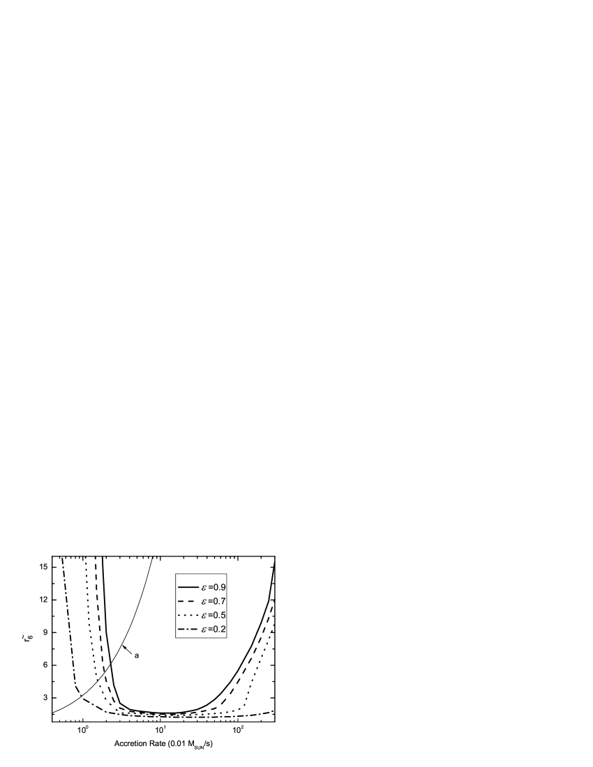
Figure 4.3: The radius $\tilde{r}$ (in units of $10^{6}$ cm) between the inner and outer disks as a function of accretion rate with different values of the energy parameter $\varepsilon$=0.9, 0.7, 0.5 and 0.2. The thin line labeled “a" is the characteristic curve of equilibrium as in Fig. 1 with $\alpha$=0.1.

In Figure 4.3, we show the inner disk size for four values of the energy parameter $\varepsilon$=0.9, 0.7, 0.5 and 0.2. We still fix $\alpha$=0.1 in this chapter in order to see the effects of advection in the inner disk with $\varepsilon<1$. This is because the size of the inner disk becomes smaller for lower $\varepsilon$, as more heating energy can be advected onto the neutron star surface, and the inner disk size is small enough to keep energy balance between heating and cooling in the disk.

Compared with the entropy-conservation self-similar structure, the size of the advection-dominated inner disk is much larger for a low accretion rate when most part of the disk is advection-dominated. When the accretion rate is low, the adiabatic index of the accreting matter is $\gamma\simeq 4/3$ and the entropy-conservation self-similar structure (4.25) can be approximately taken as $\rho\propto r^{-3}$ and $P\propto r^{-4}$, which requires a more dramatic change of density and pressure than those of the advection-dominated inner disk $\rho\propto r^{-3/2}$ and $P\propto r^{-5/2}$. This difference in structure between entropy-conservation and advection-dominated inner disks makes the size of the inner disks be different with each other.

Finally, what we should point out is that the structure of the advection-dominated self-similar inner disk even with $\varepsilon\rightarrow 1$ is different from the entropy-conservation disk with $\varepsilon=1$, since these two types of self-similar structure are based on different sets of conservation equations. The advection-dominated structure is based on the mass continuity, radial momentum and angular momentum equations, while we do not consider the local energy equation in which $Q^{+}=Q^{+}_{\rm vis}+Q^{+}_{\rm adv}$ with $Q^{+}_{\rm adv}$ to be difficult to determine locally, and we only consider the global energy equation (4.13) to calculate the size and structure of the inner disk. On the other hand, under the energy-conservation condition $Tds=0$, we can establish the relation $P\propto\rho^{\gamma}$ from the local energy equation and obtain the self-similar structure (4.25) with a combination of the mass continuity and the radial momentum and local energy equations (ZD08). However, the relation $P\propto\rho^{\gamma}$ and the integrated angular momentum equation (4.4) cannot be both satisfied in the entropy-conservation solution at the same time. In other words, the angular momentum transfer in the inner disk with the structure $P\propto\rho^{\gamma}$ cannot be merely due to the viscosity. We should consider the external torque acted on the disk or the angular momentum redistribution in the inner disk. We will discuss the entropy-conservation structure in more details in §4.5.

4.3.3 Inner Disks with Outflows

In §4.3.1 and §4.3.2, we do not consider outflows, which may have important effects on the structure and energy flux distribution of the entire disk in some cases. Following Narayan & Yi (1994, 1995) and Medvedev (2004), if the adiabatic index $\gamma<3/2$, then the Bernoulli constant of the accretion flow is positive and a thermally-driven wind or outflow can be produced from the disk. Therefore, the outflow component can be important in ADAFs. On the other hand, since the accretion rate of the neutron-star disk is very large, it is reasonable to assume that the neutron star, which has a solid surface and is different from the black hole, cannot accumulate all of the accreting matter at once, and thus an outflow could be produced near the neutron star surface and exist in the inner region of the disk.

In this section, we consider the disk structure and neutrino emission in the disk with an outflow. We consider two models depending on two mechanisms. In the first model (hereafter model O1), an outflow is mainly produced in the process of disk matter accreting onto the surface of a neutron star. We assume that only the inner disk produces an outflow and the accretion rate of the outer disk can still be considered as a constant. We take

$$\dot{M}(r)=\dot{M}_{0}(r/\tilde{r})^{s}$$ (4.31)

for the inner disk with $s$ to be the outflow index and $\dot{M}_{0}$ to be the constant accretion rate in the outer disk. Second, if an outflow is produced by the accretion process in the disk, then we consider that the outflow is produced in the entire disk (hereafter model O2 in this section), i.e.,

$$\dot{M}(r)=\dot{M}_{0}(r/r_{out})^{s}$$ (4.32)

Strictly speaking, a thermally-driven outflow from the entire disk is expected in the advection-dominated disk but not in the neutrino-dominated disk. The winds from the disks which emit a sufficient high neutrino luminosity are considered to be driven due to neutrino irradiation (Metzger et al. 2008). We adopt equation (4.32) for all the disks with a wide range of the accretion rate in model O2 for simplicity, and we also take the index $s$ of the outflow as a constant. The angular momentum equation with an outflow can be written as

$$\Sigma\nu=\frac{1+2s\zeta}{1+2s}\frac{\dot{M}}{3\pi}\left(1-\sqrt{\frac{r_{*}}{r}}\right)$$ (4.33)

where $\zeta$ describes a difference between outflow velocity $v_{outflow,\phi}$ and accretion-disk velocity $v_{\phi}$: $v_{\phi}-v_{outflow,\phi}=\zeta v_{\phi}$. From equation (4.33), we see that if $s=0$ or $\zeta=1$, i.e., there is no outflow or the toroidal velocity of the outflow is zero and no angular momentum is taken away by the outflow, then the angular momentum equation (4.33) switches back to the common case of equation (4.4). In this section, we take $\zeta=0$, i.e., $v_{outflow,\phi}\approx v_{acc,\phi}$.

With the outflow in the inner disk, the self-similar structure becomes

$$\rho\propto r^{s-3/2},\,\,P\propto r^{s-5/2},\,\,v_{r}\propto r^{-1/2}.$$ (4.34)

The energy conservation equation of the inner disk can be rewritten as

$$\int_{r_{*}}^{\tilde{r}}Q_{\nu}^{-}2\pi rdr=\varepsilon\left[\int_{r_{*}}^{\tilde{r}}\frac{9}{8}\nu\Sigma\frac{GM}{r^{3}}2\pi rdr+(1-\bar{f}_{\nu})\int_{\tilde{r}}^{r_{out}}\frac{9}{8}\nu\Sigma\frac{GM}{r^{3}}2\pi rdr\right],$$ (4.35)

where we still keep the advection parameter $\varepsilon$. For model O1 that the outflows merely exist in the inner disk due to the neutron star surface, using equations (4.31) and (4.33), we derive the energy conservation equation (4.35) as

$$\frac{1}{\varepsilon}\left(\int_{r_{*}}^{\tilde{r}}Q_{\nu}^{-}2\pi rdr\right) = \frac{3}{4}\left(\frac{1+2s\zeta}{1+2s}\right)\frac{GM\dot{M}_{0}}{\tilde{r}^{s}}$$ (4.36)

$$\times\left[\frac{1}{1-s}\left(\frac{1}{r_{*}^{1-s}}-\frac{1}{\tilde{r}^{1-s}}\right)-\frac{r_{*}^{1/2}}{3/2-s}\left(\frac{1}{r_{*}^{3/2-s}}-\frac{1}{\tilde{r}^{3/2-s}}\right)\right]$$

$$+(1-\bar{f}_{\nu})\frac{3GM\dot{M}_{0}}{4\tilde{r}}\left[1-\frac{2}{3}\left(\frac{r_{*}}{\tilde{r}}\right)^{1/2}\right]$$

for $s<1$, and

$$\frac{1}{\varepsilon}\left(\int_{r_{*}}^{\tilde{r}}Q_{\nu}^{-}2\pi rdr\right) = \frac{3}{4}\left(\frac{1+2s\zeta}{1+2s}\right)\frac{GM\dot{M}_{0}}{\tilde{r}}\left\{\textrm{ln}\left(\frac{\tilde{r}}{r_{*}}\right)-2\left[1-\left(\frac{r_{*}}{\tilde{r}}\right)^{1/2}\right]\right\}$$ (4.37)

$$+(1-\bar{f}_{\nu})\frac{3GM\dot{M}_{0}}{4\tilde{r}}\left[1-\frac{2}{3}\left(\frac{r_{*}}{\tilde{r}}\right)^{1/2}\right]$$

for $s=1$. Here we always consider the outflow index $s\leq 1$.

If the outflows exist in the entire disk (model O2), then we have

$$\frac{1}{\varepsilon}\left(\int_{r_{*}}^{\tilde{r}}Q_{\nu}^{-}2\pi rdr\right) = \frac{3}{4}\left(\frac{1+2s\zeta}{1+2s}\right)\frac{GM\dot{M}_{0}}{r_{out}^{s}}$$ (4.38)

$$\times\left[\frac{1}{1-s}\left(\frac{1}{r_{*}^{1-s}}-\frac{\bar{f}_{\nu}}{\tilde{r}^{1-s}}\right)-\frac{r_{*}^{1/2}}{3/2-s}\left(\frac{1}{r_{*}^{3/2-s}}-\frac{\bar{f}_{\nu}}{\tilde{r}^{3/2-s}}\right)\right]$$

for $s<1$ and

$$\frac{1}{\varepsilon}\left(\int_{r_{*}}^{\tilde{r}}Q_{\nu}^{-}2\pi rdr\right) = \frac{3}{4}\left(\frac{1+2s\zeta}{1+2s}\right)\frac{GM\dot{M}_{0}}{r_{out}}$$ (4.39)

$$\times\left\{\textrm{ln}\left(\frac{r_{out}}{r_{*}}\right)-\bar{f}_{\nu}\textrm{ln}\left(\frac{r_{out}}{\tilde{r}}\right)+2\left[\bar{f}_{\nu}+\left(\frac{r_{*}}{\tilde{r}}\right)^{1/2}-2\right]\right\}$$

for $s=1$. We should point out that, since we derive the energy equations (4.36)-(4.39) in the disk with outflow using the angular momentum equation (4.33) rather than the entropy-conservation expression (4.26), we still use the self-similar structure (4.34) to calculate the properties of the inner disk and the entire disk in the case of $\varepsilon\simeq 1$ both in models O1 and O2.

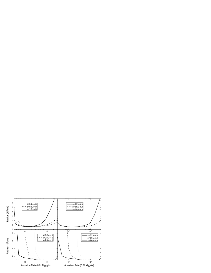
Figure 4.4: (a) Top panels: the radius $\tilde{r}$ between the inner and outer disk in model O1 with different parameter sets of the outflow index $s$=0.2, 0.6, 1 and the energy parameter $\varepsilon\simeq$ 1, 0.8. (b) Bottom panels: the radius $\tilde{r}$ in model O2 with the same parameter sets ($s,\varepsilon$) as in the top two panels.

The top two panels in Figure 4.4 show the size of the inner disk with different values of the advection parameter $\varepsilon$. In model O1, the inner disk is larger for a stronger outflow (larger $s$) with low accretion rate ($<0.2M_{\odot}s^{-1}$); but for a high accretion rate ($>0.2M_{\odot}s^{-1}$), the size of the inner disk decreases with increasing the outflow index $s$. In fact, if the accretion rate is low, the flow of the outer disk is mainly ADAF and $\bar{f}_{\nu}\sim 0$. From equations (4.36) and (4.37), most of the energy generated in the outer disk is advected into the inner region, and the inner disk size is mainly determined by the self-similar structure (4.34), which requires a less dramatic change of density and pressure as functions of radius for higher $s$ or stronger outflow. As a result, the size of the inner disk becomes larger for a stronger outflow. On the other hand, if the accretion rate is high, we have $\bar{f}_{\nu}\sim 1$ in the outer disk, the inner disk size is mainly determined by the heating energy generated in the inner disk, i.e., the first terms of the right-hand side in equations (4.36) and (4.37), and a stronger outflow carries away more energy from the disk and allows a smaller size of the inner disk when the accretion rate is sufficiently high.

The bottom two panels in Figure 4.4 show the inner disk size in model O2 in which an outflow exists in the entire disk. The inner disk structure cannot exist for a high accretion rate ($>0.4M_{\odot}s^{-1}$) except for the weak outflow case ($s=0.2$) where the inner disk also exists in some range of a high accretion rate. The change of the inner disk size is more significant for a large outflow index $s$ and even the entire accretion disk can satisfy the self-similar structure (4.33) for a sufficiently low accretion rate. For a high accretion rate ($>0.5M_{\odot}s^{-1}$), the outflow can take away enough heating energy from the disk, and a balance between heating and cooling in the entire disk can be built even without an inner disk. In this range of a high accretion rate, the structure of the neutron-star disk in model O2 is very similar to the black hole disk with an outflow.

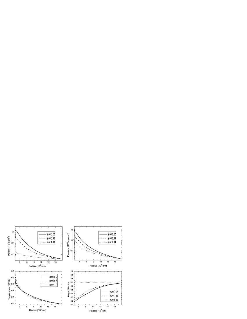
Figure 4.5: Density, pressure, temperature and height (half-thickness) as functions of radius for different values of the outflow index $s$=0.2, 0.6, 1, where we take the accretion rate as 0.2$M_{\odot}$ $\rm s^{-1}$ and the energy parameter $\varepsilon$=0.8.

Figure 4.5 shows the structure of the disk with different values of the outflow index $s$=0.2, 0.6 and 1 in model O2. We choose the accretion rate $\dot{M}=0.2M_{\odot}$ s^-1 and the energy parameter $\varepsilon$=0.8. The density and pressure in the disk decrease with increasing the outflow strength in the entire disk, and the disk becomes thicker for a stronger outflow. The change of the temperature is not as obvious as the density and pressure. Most part of the outer region of the disk will be cooler for a stronger outflow, but the inner disk region can be hotter in order to release the heating energy advected from the outer region of the disk.

Self-similar structure and size of the inner disk in various cases Cases Inner disk self-similar structure Inner disk size Case 1: $\varepsilon\simeq$1, no outflow entropy-conservation structure (4.26) Figure 4.1 Case 2: $\varepsilon<$1, no outflow advection-dominated structure (4.30) Figure 4.3 Case 3: outflow model O1 outflow structure (4.34) Figure 4.4 top panels Case 4: outflow model O2 outflow structure (4.34) Figure 4.4 bottom panels

Table 4.2: We discuss case 1 in §4.3.1, case 2 in §4.3.2, case 3 and case 4 in §4.3.3 with different inner disk structures based on energy and mass transfer in the entire disk.

We make a brief summary in the end of this section. We propose the inner disk to satisfy the self-similar structure. Table 4.2 shows the main results in this section. The inner disk satisfies the entropy-conservation self-similar structure as in ZD08 for the energy parameter $\varepsilon\simeq 1$, while it becomes an advection-dominated self-similar region for $\varepsilon<1$. In outflow model O1, an outflow is produced in the inner disk due to the prevention effect of the neutron star surface, and model O2 suggests that an outflow exists in the entire disk as in Kohri et al. (2005). We discuss the size of the inner disk depending on different structures of the inner disk and outflow and different values of the viscosity parameter.

4.4 Neutrino Annihilation

4.4.1 Calculation Method and Surface Boundary Condition

Hyperaccreting black hole disks can convert some fraction of the net accretion energy into the energy of a relativistic outflow or wind by two general mechanisms: neutrino annihilation and magnetohydrodynamical effects such as the Blandford-Znajek mechanism or magnetic instabilities. However, for hyperaccretion disks surrounding neutron stars, the energy conversion mechanism is mainly due to the neutrino annihilation for magnetic fields at the neutron star surface $\leq 10^{15}-10^{16}$ G. We consider the process of electron capture $\nu_{i}+\bar{\nu}_{i}\rightarrow e^{+}+e^{-}$ as the most important interaction for energy production. As the neutron-star disk is denser, hotter with higher pressure, and has a brighter neutrino luminosity compared with the black-hole disk in most cases, the neutrino annihilation efficiency of the neutron-star disk should be higher than that of the black-hole disk. Moreover, the surface boundary of the neutron star, which carries away gravitational-binding energy by neutrino emission, also makes the neutrino annihilation luminosity of the neutron-star disk be higher than that of the black-hole counterpart.

In this section, we follow the approximate method used by Ruffert et al. (1997, 1998) and Popham et al. (1999) to calculate the neutrino annihilation luminosity, i.e., the vertically-integrated disk is modeled as a grid of cells in two dimensions ($r,\varphi$). The symbols $\epsilon_{\nu_{i}}^{k}$ and $l_{\nu_{i}}^{k}$ are the mean neutrino energy and neutrino radiation luminosity with three different types of neutrino ($i=e,\tau,\mu$) in the cell $k$, and $d_{k}$ is the distance from the cell $k$ to a certain spatial point. The neutrino annihilation at any point above the disk is

$$l_{\nu\bar{\nu}}=\sum_{i=e,\mu,\tau}A_{1,i}\sum_{k}\frac{l_{\nu_{i}}^{k}}{d_{k}^{2}}\sum_{k^{\prime}}\frac{l_{\bar{\nu}_{i}}^{k^{\prime}}}{d_{k^{\prime}}^{2}}(\epsilon_{\nu_{i}}^{k}+\epsilon_{\bar{\nu}_{i}}^{k^{\prime}})(1-\cos\theta_{kk^{\prime}})^{2}$$

$$+\sum_{i=e,\mu,\tau}A_{2,i}\sum_{k}\frac{l_{\nu_{i}}^{k}}{d_{k}^{2}}\sum_{k^{\prime}}\frac{l_{\bar{\nu}_{i}}^{k^{\prime}}}{d_{k^{\prime}}^{2}}\frac{\epsilon_{\nu_{i}}^{k}+\epsilon_{\bar{\nu}_{i}}^{k^{\prime}}}{\epsilon_{\nu_{i}}^{k}\epsilon_{\bar{\nu}_{i}}^{k^{\prime}}}(1-\cos\theta_{kk^{\prime}}),$$ (4.40)

where the values of the neutrino cross section constants $A_{1,i}$ and $A_{2,i}$ can be seen in Popham et al. (1999). The total neutrino annihilation luminosity above the disk can be integrated as

$$L_{\nu\bar{\nu}}=2\pi\int_{r_{*}}^{\infty}dr\int_{H}^{\infty}l_{\nu\bar{\nu}}rdz.$$ (4.41)

For a neutron-star disk, we should consider both its different structure compared with the black-hole disk and the boundary condition of the neutron star surface layer. The neutrino annihilation luminosity is not only contributed by neutrinos emitted from the disk but also from the neutron star surface layer. The luminosity available to be radiated by the boundary layer at neutron star surface is (Frank et al. 2002)

$$L_{s}=\frac{1}{4}\dot{M}r_{*}^{2}(\Omega_{K}^{2}-\Omega_{*}^{2})-G_{*}r_{*}\simeq\frac{GM\dot{M}}{4r_{*}}\left(1-\frac{\Omega_{*}}{\Omega_{K}}\right)^{2},$$ (4.42)

where $\Omega_{*}$ is the angular velocity of the neutron star surface, and $G_{*}\simeq\frac{1}{2}\dot{M}r_{*}^{2}(\Omega_{K}-\Omega_{*})$ is the viscous torque acted on the accretion disk. Here we only study the vertically integrated disk over a half-thickness (height) $H$. As a result, the luminosity is a function of accretion rate $\dot{M}$ and neutron star surface angular velocity $\Omega_{*}$. In the case where the inner disk satisfies the entropy-conservation self-similar structure, we introduce the efficiency factor $\eta_{s}$ to measure the energy emitting from the neutron star surface and rewrite equation (4.42) as

$$L_{s}=\eta_{s}\frac{GM\dot{M}}{4}\left(\frac{1}{r}-\frac{1}{r_{out}}\right).$$ (4.43)

If $\Omega_{*}\sim\Omega_{K}$, we have $\eta_{s}\sim 0$ and there is no emission from the surface layer; or if $\Omega_{*}\sim 0$, we have $\eta_{s}\sim 1$, which satisfies the Virial condition. We consider the energy released from the surface layer is mainly carried away by neutrino emission, and thus the neutrino emission rate and the temperature at the layer are related by

$$Q_{\nu,s}=\frac{\eta_{s}}{2\pi r_{*}H_{*}}\frac{GM\dot{M}}{4}\left(\frac{1}{r_{*}}-\frac{1}{r_{out}}\right)\sim\frac{7}{8}\sigma_{B}T^{4}.$$ (4.44)

In the case where the self-similar inner disk is advection-dominated, we obtain the gravitational energy released by neutrino emission as

$$L_{s}=\eta_{s}\frac{GM\dot{M}}{4}\left(\frac{1}{r}-\frac{1}{r_{out}}\right)+(1-\varepsilon)\frac{GM\dot{M}}{4}\left\{\frac{1}{r_{*}}-\bar{f}_{\nu}\left[1-\frac{2}{3}\left(\frac{r_{*}}{\tilde{r}}\right)^{1/2}\right]\right\},$$ (4.45)

where the second term in the right side of equation (4.45) is the heating energy advected from the inner disk to the surface boundary layer, and we can further write equation (4.45) as

$$L_{s}=(\eta_{s}+\eta_{s,ADAF})\frac{GM\dot{M}}{4}\left(\frac{1}{r}-\frac{1}{r_{out}}\right),$$ (4.46)

where we take the equivalent factor $\eta_{s,ADAF}$ to measure the energy advected from the advection-dominated inner disk to the surface boundary. Table 4.3 shows examples of $\eta_{s,ADAF}$ with different inner disk structures.

Equivalent factor $\eta_{s,ADAF}$ with different inner disk structures $\eta_{s,ADAF}$ 0.03 0.1 0.3 0.5 1.0 3.0 ($M_{\odot}$ s^-1) $\varepsilon$=0.9 9.07e-2 5.25e-2 4.22e-2 5.56e-2 7.75e-2 9.56e-2 $\varepsilon$=0.5 0.419 0.196 0.159 0.149 0.180 0.446 $\varepsilon$=0.2 0.675 0.496 0.219 0.178 0.218 0.382 O1: $s$=0.2 0.228 0.113 7.84e-2 8.72e-2 0.107 0.202 $s$=0.6 – 0.215 0.115 0.113 0.119 0.209 $s$=1.0 – 0.315 0.199 0.168 0.203 0.336 O2: $s$=0.2 0.238 0.104 7.95e-3 – – – $s$=0.6 – 0.428 5.79e-4 – – – $s$=1.0 – – 0.639 4.36e-4 – –

Table 4.3: Equations (4.45) and (4.46) give the value of $\eta_{s,ADAF}$. We choose cases of the advection-dominated inner disk with $\varepsilon$=0.9, 0.5, 0.2, and models O1 and O2 with $s$=0.2, 0.6 1.0 to calculate $\eta_{s,ADAF}$.

When an outflow exists in the disk, the luminosity at the boundary surface is dimmer since the accretion rate near the neutron star surface is lower due to the outflow. We can modify equation (4.45) by changing the accretion rate $\dot{M}$ to be $\dot{M}_{0}(r_{*}/\tilde{r})^{s}$ for model O1 in §3.3 and $\dot{M}_{0}(r_{*}/r_{out})^{s}$ for model O2.

4.4.2 Results of Annihilation Luminosity

We calculate the neutrino annihilation luminosity $L_{\nu\bar{\nu}}$ and the total neutrino luminosity $L_{\nu}$ emitted from the disk and neutron star surface. The results of $L_{\nu\bar{\nu}}$ and $L_{\nu}$ depend on the value of the viscosity parameter $\alpha$, the detailed structure of the inner disk, the strength of the outflow, as well as the neutron star surface boundary condition. We discuss the effects of these various factors in Figure 4.6 to Figure 4.9.

Figure 4.6: Neutrino annihilation luminosity $L_{\nu\bar{\nu}}$ (thick lines) and total neutrino emission luminosity $L_{\nu}$ (thin lines) as functions of accretion rate. The solid lines correspond to the neutron-star disk with the entropy-conservation inner disk and the boundary layer emission efficiency $\eta_{s}=0$, the dashed lines to the neutron-star disk with the boundary condition $\eta_{s}=0.5$, and the dotted lines to the black-hole disk.

Figure 4.6 shows the total neutrino annihilation luminosity $L_{\nu\bar{\nu},NS}$ and the emission luminosity $L_{\nu,NS}$ of the neutron-star disk with different surface boundary layer conditions ($\eta_{s}$=0 and 0.5), and we compare them with the black-hole disk. In this figure we take the neutron-star inner disk structure to satisfy the entropy-conservation self-similar structure (4.26). The total luminosity and annihilation luminosity of the neutron-star disk are brighter than those of a black-hole disk with the same mass and accretion rate. If we study the neutrino annihilation from the entire disk without surface boundary emission ($\eta_{s}$=0), the difference between $L_{\nu\bar{\nu},NS}$ and $L_{\nu\bar{\nu},BH}$ is more significant for a low accretion rate than for a high accretion rate. We have mentioned the reason in ZD08 that a larger inner disk for a neutron-star disk with a low accretion rate makes the neutrino luminosity much brighter than its black hole counterpart, and the annihilation rate also becomes higher for the neutron-star disk. For a high accretion rate ($>$0.5$M_{\odot}$ s^-1), the effect of neutrino opacity on $L_{\nu,BH}$ and $L_{\nu\bar{\nu},BH}$ also be less than that on $L_{\nu,NS}$ and $L_{\nu\bar{\nu},NS}$. On the other hand, neutrino emission from the neutron star surface boundary layer ($\eta_{s}$=0.5) makes the annihilation luminosity be more than one order of magnitude higher than that without boundary emission ($\eta_{s}$=0). $L_{\nu\bar{\nu}}$ reaches 10⁵⁰ ergs s^-1 when $\dot{M}\sim 1M_{\odot}$ s^-1 for a black-hole disk or neutron-star disk with $\eta_{s}$=0, but only needs $\dot{M}\sim 0.1M_{\odot}$ s^-1 for a neutron-star disk with the boundary condition $\eta_{s}$=0.5. Therefore, a lower-spin neutron star with hyperaccreting disk around it could have an obviously higher annihilation efficiency than that of a higher-spin neutron star. We will discuss the neutrino annihilation luminosity of a neutron-star disk in more details in §4.5.

Figure 4.7: Neutrino annihilation luminosity $L_{\nu\bar{\nu}}$ and the total neutrino luminosity $L_{\nu}$ with different values of the viscosity parameter $\alpha$ and energy parameter $\varepsilon$. The thin lines correspond to $\eta_{s}=0$ and thick lines to $\eta_{s}=0.5$. (a) Left panel: $L_{\nu\bar{\nu}}$ with $\alpha$=0.1 (solid line), 0.01 (dashed line), 0.001 (dotted line) and total luminosity $L_{\nu}$ (dash-dotted line), where we take $\varepsilon=1$ and the entropy-conservation inner disk structure. (b) Right panel: $L_{\nu\bar{\nu}}$ of the neutron-star disk with advection-dominated inner disk and $\varepsilon$=0.9 (solid line), 0.5 (dashed line), 0.1 (dotted line) and the total luminosity $L_{\nu}$ (dash-dotted line).

In Figure 4.7, we show the total neutrino annihilation luminosity of a neutron star disk with different values of the viscosity parameter $\alpha$=0.1, 0.01, 0.001 and the energy parameter $\varepsilon$=0.9, 0.5, 0.1. The disk with a moderate viscosity parameter ($\alpha$=0.01) has the highest annihilation efficiency and luminosity for a low accretion rate, and the annihilation luminosity from a high-$\alpha$ disk ($\alpha$=0.1) becomes the brightest for an accretion rate $\dot{M}\geq 0.05M_{\odot}$ s^-1. As discussed in Figure 4.2, a low-$\alpha$ disk has a brighter neutrino luminosity $Q_{\nu}$, but it is thinner than a high-$\alpha$ disk. These two competitive factors lead to the annihilation results shown in Figure 4.7a. Figure 4.7b shows that the annihilation efficiency increases with increasing $\varepsilon$. This is because the disk with lower $\varepsilon$ means more heating energy in the disk to be advected onto the neutron star surface and increases the neutrino luminosity of the surface layer, and the value of $\eta_{s,ADAF}$, which plays an important role in increasing the annihilation efficiency of the entire disk.

Figure 4.8: Neutrino annihilation luminosity $L_{\nu\bar{\nu}}$ of the neutron-star disk with outflow index $s$=0.2 (solid line), 0.6 (dashed line), 1.0 (dotted line) and the maximum value of total luminosity $L_{\nu}$ in the case of $s$=0.2 (dash-dotted line), where we take $\varepsilon$=0.8. Left panel shows the results of model O1 and right panel to model O2. The thin lines correspond to the luminosity to $\eta_{s}=0$ and thick lines to $\eta_{s}=0.5$.

Figure 4.8 shows the total neutrino annihilation luminosity $L_{\nu\bar{\nu}}$ of the disk with an outflow. We consider the results of model O1 in which an outflow only exists in the inner disk due to the neutron star surface and of model O2 in which an outflow exists in the entire disk. The difference in annihilation luminosity with different values of the outflow index $s$ but the same surface boundary condition is not obvious in model O1. However, $L_{\nu\bar{\nu}}$ becomes much dimmer for a high outflow index $s$ in model O2, which means a strong outflow in the entire disk and decreases the neutrino annihilation efficiency significantly.

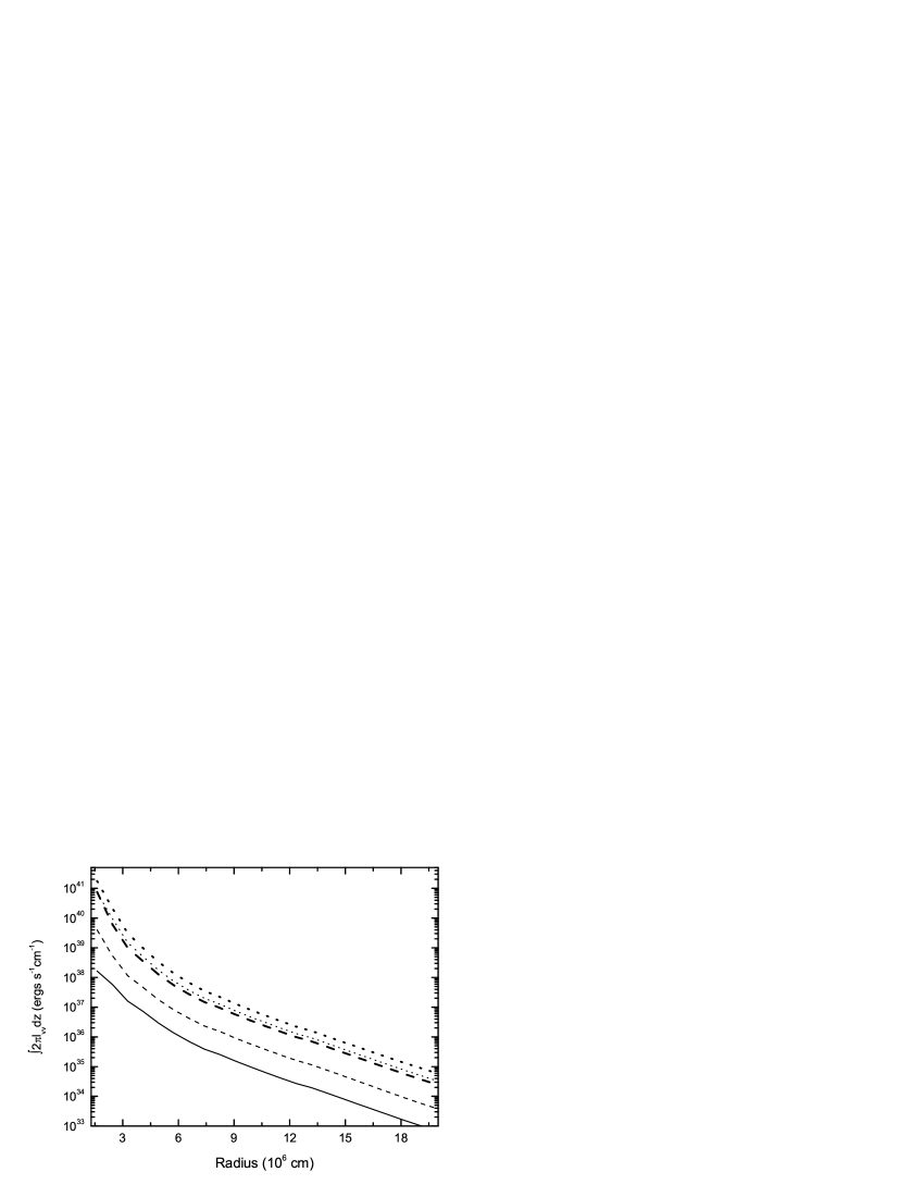
Figure 4.9: Neutrino annihilation luminosity per cm distribution as a function of radius for $\dot{M}$=0.01$M_{\odot}$ s^-1 (left panel) and $\dot{M}$=0.1$M_{\odot}$ s^-1 (right panel). (a) Left panel: annihilation luminosity per cm for a black-hole disk (thin solid line), neutron-star disks with entropy-conservation inner disk and $\eta_{s}$=0 (thin dashed line), and $\eta_{s}$=0.5 (thick dashed line), and neutron-star disks with advection-dominated inner disk $\varepsilon$=0.2 and $\eta_{s}$=0 (thin dotted line), and $\varepsilon$=0.2 and $\eta_{s}$=0.5 (thick dotted line). (b) Right panel: annihilation luminosity per cm for a neutron-star disk with outflow (model O2) $\varepsilon$=1, $s$=0.6, $\eta_{s}$=0 (thin dotted line), $\varepsilon$=1, $s$=0.6, $\eta_{s}$=0.5 (thick dotted line). The thin solid line, thin dashed line and thick dashed line are the same as the left panel.

Furthermore, we study the spatial distribution of the neutrino annihilation luminosity. Figure 4.9 illustrates the integrated annihilation luminosity per cm distribution

$$2\pi r\int_{H}^{\infty}l_{\nu\bar{\nu}}dz$$ (4.47)

for two accretion rates $\dot{M}$=0.01$M_{\odot}$ s^-1 and 0.1$M_{\odot}$ s^-1 with different physical structures of the disk. We find that the integrated annihilation luminosity drops dramatically along the disk radius, and a majority of the annihilation energy is ejected from the cylindric region above the disk with $r<3\times 10^{6}$cm. The difference of the integrated luminosity per cm between the black-hole disk and neutron-star disk is more significant for a low accretion rate when the inner entropy-conservation disk is sufficiently large. The luminosity of the neutron-star disk with an advection inner disk can be about four orders of magnitude higher than its black-hole counterpart to produce a jet with higher energy, while an outflow makes the annihilation luminosity above the neutron-star disk be lower than that of the black-hole disk.

Compared with the black-hole disk, the neutron-star disk could produce a brighter neutrino flux and more powerful annihilation luminosity. However, the mass-loss rate driven by neutrino-on-baryon absorption reactions (Qian & Woosley 1996) along the polar axis of the neutron-star disk is also significantly higher than its black-hole counterpart. This raises the problem of whether simultaneously more powerful annihilation luminosity and higher mass loss rate could work together to produce a relativistic jet required for the GRB phenomena. For example, a heavily baryon-loaded wind from a new-born neutron star within 100 ms prevents any production of a relativistic jet (Dessart et al. 2009). However, a weaker wind above the polar region and spherical asymmetry of the outflow at late times could make production of a relativistic jet above the stellar pole become possible. We will discuss this issue in more details in §4.5.3.

4.5 Discussions

4.5.1 Size of the Inner Disk

In §4.3 we study various self-similar structures of the inner disk. In this section we first want to discuss the entropy-conservation structure. The inner disk can be determined by the self-similar structure (4.26) and the energy equation (4.13). However, the inner disk with the entropy-conservation structure cannot satisfy the integrated angular momentum equation (4.4). There are two explanations. First, we can consider the term $d\dot{J}_{ext}/dr\neq 0$ in equation (4.3) for a steady-state disk since the angular momentum redistributes in the inner disk before the entire disk becomes steady-state. As mentioned in ZD08, because the neutron star surface prevents heating energy from being further advected inward, the inner disk is formed to balance the heating and cooling energy in the entire disk. As a result, energy and angular momentum could redistribute in the inner disk. Second, besides this consideration on angular momentum redistribution, we can also discuss another type of inner disk with the entropy-conservation structure discussed by Medvedev & Narayan (2000), which still satisfies the angular momentum equation (4.4) with $v_{r}\ll v_{K}$ and $\Omega\simeq$constant. The angular momentum transfer and heating energy generation due to viscosity can be neglected in the inner disk, as $\Omega$ is approximately equal to an constant, and the heating energy in the inner disk is merely the energy advected from the outer disk, i.e., $Q^{+}=Q^{+}_{\rm adv}$ in the inner disk. As a result, the global inner-disk energy conservation equation (4.13) should be modified as

$$\int_{r_{*}}^{\tilde{r}}Q_{\nu}^{-}2\pi rdr=\frac{3GM\dot{M}}{4}\left\{{\frac{1}{3\tilde{r}}-\frac{\bar{f}_{\nu}}{\tilde{r}}\left[1-\frac{2}{3}\left(\frac{r_{*}}{\tilde{r}}\right)^{1/2}\right]}\right\},$$ (4.48)

for $\Omega\simeq{\rm constant}=\Omega(\tilde{r})$ in the inner disk. Compared with equation (4.13), equation (4.48) requires a smaller value of $\tilde{r}$ with the same neutron star mass and accretion rate.

Figure 4.10: The radius $\tilde{r}$ (in units of $10^{6}$ cm) between the inner and outer disks with the viscosity parameter $\alpha$=0.1 (solid line) and 0.01 (dashed line). The thick lines show the results based on the consideration $\Omega\simeq$ const in the inner disk in §5, and the thin lines based on the angular velocity distribution $\Omega\propto r^{-3/2}$ as in §3.

Figure 4.10 shows the value of $\tilde{r}$ for $\alpha$=0.1 and 0.01 with $\Omega\simeq$constant and $\Omega\propto r^{-3/2}$. The constant angular velocity in the inner disk decreases the inner disk size compared to the case of $\Omega\propto r^{-3/2}$. However, in order to get a unified scenario of the entire disk in various cases, we adopt $\Omega\propto r^{-3/2}$ for all the self-similar structures in §4.3.

4.5.2 Annihilation Results and Disk Geometry

Several previous studies have been performed to calculate the neutrino annihilation efficiency above the disk around a black hole with the effects of disk geometry, gravitational bending, rotation of central black holes and so on (e.g., Ruffert et al. 1997, 1998; Popham et al. 1999; Asano & Fukuyama 2000, 2001; Miller et al. 2003; Birkl et al. 2007). The simulations based on general relativity show the effects of general relativity such as the Kerr black holes and bending neutrino geodesics in spacetime increase the total annihilation rate by a factor of a few. Also, compared with the spherical and torus neutrinosphere, the disk neutrinosphere with the same temperature and neutrino luminosity distribution usually have the highest annihilation efficiency (Birkl et al. 2007). In this chapter, we still adopt the calculation approach on annihilation based on Ruffert et al. (1997, 1998) and Popham et al. (1999), and consider the vertically-integrated Newtonian disk. The most important results of annihilation calculation in our work is that the neutron-star disk produce more energetic annihilation luminosity compared to the black-hole counterpart. Moreover, we consider neutrinos emitted from the stellar surface region, and the neutrino emission concentrated in this surface region plays a significant role in increasing the annihilation luminosity to produce relativistic ejecta formed by $e^{+}e^{-}$ plasma. On the other hand, we should note that the effect of surface boundary condition emission could be reduced if the emission region becomes larger than we consider in this chapter due to outflow or the other cooling mechanisms rather than neutrino cooling at the surface. Some other works focusing on neutrino annihilation in supernovae discussed neutrino emission from the entire spherical neutron star surface (Cooperstein et al. 1986; Goodman et al. 1987; Salmonson & Wilson 1999). Therefore, a further work should be done to study the effects of boundary emission and cooling based on more elaborate considerations on cooling mechanisms and energy transfer at the boundary around neutron-star disk. However, as the neutron-star disk and the surface emission increase the annihilation luminosity more significantly than the general relativity effects, we conclude our main results would maintain for more elaborate simulations based on advanced calculations on neutrino annihilation above the disk.

4.5.3 Application to GRB Phenomena

Energy can be deposited in the polar region of black-hole and neutron-star disks by neutrino annihilation and MHD processes. We focus on the annihilation process in this chapter. In the black-hole case, the environment along the polar axis (i.e., the rotation axis of the disk around neutron star) can be baryon-free. For example, GRB can commence after the initial collapse for $\sim 15$ s in the collapsar scenario, when the accretion process in the polar region becomes sufficiently weak to produce a relatively clean environment with the mass density $\leq 10^{6}$ g cm^-3 (MacFadyen & Woosley 1999). In the neutron-star case, however, the enormous neutrino luminosity of a neutron star would drive appreciable mass-loss from its surface during the first 20 s of its life (Qian & Woosley 1996). The wind material will feed the polar region, where a large amount of annihilation energy is deposited. Dessart et al. (2009) showed that a newly formed neutron star from the neutron star binary merger will develop a powerful neutrino-driven wind in the polar funnel in a few milliseconds after its formation. The mass-loss associated with the neutrino-driven wind is on the order of $10^{-3}M_{\odot}$ s^-1, preventing energy outflow from being accelerated to relativistic speed and producing a GRB. Their numerical simulations stops at $t\sim 100$ ms, while they considered that the neutron star will collapse to a black hole quickly. However, a stable neutron star with much longer lifetime $\gg 100$ ms has also been proposed as the GRB central engine. A rapidly rotating neutron star formed by the neutron star binary merger (Gao & Fan 2006) or the merger of a white dwarf binary (King et al. 2001) could produce extended emission (Metzger et al. 2008b) or X-ray flares (Dai et al. 2006) about 10-100 s afetr the neutron star birth, and last for tens of seconds. In the collapsar scenario, a newly formed neutron star or a magnetar could also form after the initial collapse or associated supernova explosion, and the lifetime of the neutron star before collapsing to a black hole can reach as long as several months to yrs (Vietri & Stella 1998). Therefore, many GRB models lead to a longtime ($\gg 100$ ms) neutron star, which can produce other phenomena accompanying the GRB prompt emission. On the other hand, the accretion timescale can last for longer than 10s in the collapse process of a massive star, or for several seconds after the merger of a compact star binary with the disk viscosity parameter $\alpha<0.1$ (Narayan et al. 2001). Thus we can discuss the steady-state scenario of a neutron star with lifetime $\gg 100$ ms surrounded by a hyperaccreting disk.

For a longtime neutron star, the strengthen of a neutrino-driven winds above the stellar polar region would drop quickly at late times, as the total mass-loss rate $\dot{M}\sim t^{-5/3}$, and the neutrino-driven wind become weaker above the polar region than that from the low latitudes and midplane region of the neutron star. It is difficult to calculate the spatial distribution of Lorentz factor of the outflow material above the polar region precisely in our present work, because we only use the approximate disk geometry to calculate the steady-state spatial distribution of the neutrino annihilation efficiency. We do not simulate the dynamical evolution of the neutrino-driven wind. However, we can estimate the speed of outflow material using semi-analytic methods as follows. The mass loss rate for a thermal neutrino-driven wind can be approximately given by (Qian & Woosley 1996)

$$\dot{M}_{\rm wind}\approx 1.14\times 10^{-10}C^{5/3}L_{\bar{\nu}_{e},51}\epsilon_{\nu_{e},MeV}^{10/3}(r/10^{6}\textrm{cm})^{5/3}(M/1.4M_{\odot})^{-2}M_{\odot}\,\textrm{s}^{-1},$$ (4.49)

where $10^{51}$$L_{\bar{\nu}_{e},51}$ergs s^-1 is the luminosity of the $\bar{\nu}_{e}$ emission, $\epsilon_{\nu_{e}}$=1MeV$\epsilon_{\nu_{e},MeV}$ is the mean neutrino energy of the neutron star surface, and $C\approx 1+0.733(r/10^{6}\textrm{cm})^{-1}(M/1.4M_{\odot})$. Thus the typical steady state spherical mass-loss rate due to thermal neutrino absorption reactions for a neutron star with 10km radius is on the order of a few $10^{-6}-10^{-5}M_{\odot}$ s^-1, depending on the initial configuration of the material above the neutron star surface (i.e., Qian & Woosley 1996, Tab. 1). The mass-loss rate depends on the neutrino luminosity and temperature above the neutron star surface sensitively. When the neutron star with weak magnetic field $<10^{15}$ G is surrounded by a hyperaccreting disk, the neutron star surface should have a higher temperature near the star midplane than its polar region, as mentioned in the last section §4. Thus the neutron star should produce a stronger wind above the midplane region than above its poles. As a result, the mass-loss rate via neutrino absorption above the star polar region is estimated as

$$\dot{M}_{\rm polar}=\dot{M}_{\rm wind}\left(\frac{\Delta\Omega}{2\pi}\right)f_{asy},$$ (4.50)

where $\Delta\Omega=\int\textrm{cos}\varphi d\varphi d\phi$ is the solid angle of the polar funnel, and $f_{asy}<1$ is used to measure the degree of spherical asymmetry. Moreover, the bulk Lorentz factor of the outflows from the neutron star surface is

$$\Gamma\geq\frac{L_{\nu\bar{\nu}}f_{k}}{\dot{M}_{\rm polar}c^{2}}=\frac{L_{\nu\bar{\nu}}}{\dot{M}_{\rm wind}c^{2}}\left(\frac{2\pi f_{k}}{\Delta\Omega f_{asy}}\right),$$ (4.51)

where $f_{k}$ is the fraction of deposited annihilation energy which provides kinetic energy of the neutron star wind above the polar region. We can estimate whether the outflow material from the polar region of the neutron star surface can be accelerated to a relativistic speed using equation (4.51). Here we take the bulk Lorentz factor $1<\Gamma<10$ as a mildly relativistic speed, $10\leq\Gamma<100$ as a moderately relativistic speed and $\Gamma>100$ as an ultrarelativistic speed. If we take the bulk Lorentz factor $\Gamma$ as a parameter, the solid angle of the polar region $\Delta\Omega/2\pi\sim 0.1$, and $f_{k}\sim f_{asy}$, then we can estimate the upper limit of total thermal mass-loss rate from the neutron star surface with particular boundary layer conditions, and compare such limits with the actual mass-loss rate of thermal neutrino-driven winds calculated by equation (4.49). In Figure 4.11 we explore the possibility of producing a relativistic jet. We show the maximum allowed strength of total mass-loss for the wind material above the polar region being accelerated to $\Gamma=10$ and $\Gamma=100$ with the chosen boundary layer condition $\eta_{s}=0$ and $\eta_{s}=0.5$ as in §4.4. The neutrino emission from the neutron star surface layer increases the neutrino annihilation luminosity and efficiency, while it increases the stellar surface mass-loss simultaneously.

Figure 4.11: Upper limit of mass-loss rate due to neutrino-driven wind from the neutron star surface for the outflow being accelerated to $\Gamma=10$ (moderately relativistic) with the surface emission boundary condition $\eta_{s}=0$ (thin solid line) or $\eta_{s}=0.5$ (thin dashed line); or $\Gamma=100$ (ultrarelativistic) with the surface emission boundary condition $\eta_{s}=0$ (thick solid line) or $\eta_{s}=0.5$ (thick dashed line). The dotted lines “a" and “b" correspond to the strength of a thermally neutrino-driven wind from the stellar surface for the boundary condition $\eta_{s}=0$ and $\eta_{s}=0.5$ respectively.

From Figure 4.11, we find that moderately relativistic outflows above the neutron star polar region are possible under some cases, e.g., the wind material can be accelerated to $10<\Gamma<100$ above the polar region for the disk accretion rate $\dot{M}\geq 0.08M_{\odot}$ s^-1 with $\eta_{s}=0.5$. This result can still be kept for other values of $f_{k}/f_{asy}$ around unit. However, annihilation process can never produce any winds with bulk Lorentz factor $\Gamma\geq 100$, as the heavily mass-loaded neutron-star wind precludes ultrarelativistic speed even for very high annihilation efficiency with sufficiently bright neutrino emission from the innermost disk radius. Zhang et al. (2003, 2004) found that relativistic jets formed in the accreting black hole systems can be collimated by their passage through the stellar envelope; moderately and even mildly relativistic jets can be partly accelerated to an ultrarelativistic speed after they break out in the massive star, because the jets’ internal energy can be converted to kinetic energy after jet breakout. Such jet-stellar-envelope interactions also happen around the hyperaccreting neutron star systems, although the neutron-star disk systems can be surrounded by a cavity $\sim 10^{9}$ cm inside the progenitor stars with the stellar radius of several $10^{10}$ cm (e.g., Bucciantini et al. 2008, 2009). In the compact star binary merger scenario, on the other hand, a moderately relativistic jet is possible to produce a short-duration GRB.

As a result, the neutron-star disk can produce a sufficiently larger annihilation luminosity than its black-hole counterpart. However, a neutrino-driven outflow from the newly formed neutron star at early times ($\sim 100$ ms) is so heavily mass-loaded that it can in no way be accelerated to relativistic speed. For a longtime neutron star, however, mass-loss becomes weaker above the stellar pole than above the low latitudes and midplane. Thus a moderately relativistic jet can be produced in a hyperaccreting neutron-star system with sufficiently high disk accretion rate and bright boundary emission (e.g., the accretion rate $\dot{M}\geq 0.08M_{\odot}$ s^-1 for $\eta_{s}=0.5$). Also, the jet can be collimated by jet-stellar-envelope interactions, and partly accelerated to an ultrarelativistic speed after jet breakout if the neutron star forms through stellar collapse. Therefore, some hyperaccreting neutron-star system can produce GRBs, which are more energetic than those from the black-hole systems. We know that some long-duration GRBs can reach a peak luminosity of $\sim 10^{52}$ ergs s^-1 (e.g. GRB 990123, Kulkarni et al. 1999), which requires a very high accretion rate $\sim 10M_{\odot}$ s^-1 as well as a much more massive disk ($\geq 10M_{\odot}$) around a black hole compared to the typical disk or torus mass $0.01-1M_{\odot}$ if the energy is provided by neutrino annihilation above the black-hole disk. However, if we consider the neutron-star disk with the surface boundary emission (e.g. $\eta_{s}\sim 0.5$), we only need an accretion rate $\sim 1M_{\odot}$ s^-1 onto the neutron star, which is one order of magnitude less than that of the black-hole disk, and the disk mass can be $\sim 1M_{\odot}$ for a long burst with the peak luminosity $10^{52}$ ergs s^-1 in a time of about 1s. However, other reasons or mechanisms such as the jet effect to reduce the total burst energy or the magnetic mechanism rather than neutrino annihilation to provide the GRB energy have been introduced into the GRB central engine models. Therefore, it is necessary to search new important observational evidence to show the existence of a central neutron star rather than black hole surrounded by a hyperaccreting disk. X-ray flares after GRBs may be a piece of evidence, which shows that an activity of the central neutron star after the burst may be due to magnetic instability and reconnection effects in differentially-rotating pulsars (Dai et al. 2006). However, more studies should be done to compare other models of X-ray flares (King et al. 2005; Proga & Zhang 2006; Perna et al. 2005; Lee & Ramires-Ruiz 2007, Lazzati et al. 2008) with the differential-rotating pulsar model and show more effects of such a magnetized pulsar. For example, the spin-down power of a magnetar probably explains the peculiar optical to X-ray integrated luminosity of GRB 060218 (Soderberg et al. 2006).

Furthermore, we propose that other GRB-like events may be produced by hyperaccreting neutron star systems, if winds fail to reach a proper relativistic speed. As mentioned by MacFadyen et al. (2001), a mildly or moderately relativistic jet may lead to X-ray flashes, which are less energetic than normal GRBs. This will also happen in the neutron-star case. Another possible result is that a heavily mass-loaded wind with nonrelativistic speed could produce a bright SN-like optical transient event (Kohri et al. 2005; Metzger et al. 2008a).

4.5.4 GRB-SN Association

Besides GRBa and GRB-like phenomena, we think a nonrelativistic or mildly relativistic outflow from a hyperaccreting disk and neutron star surface may feed a supernova explosion associated with a GRB. The discovery of connection between some GRBs and supernovae has inspired studies of the origin of GRB-SN association (e.g., Iwamota et al. 1998; MacFadyen & Woosley 1999; Zhang et al. 2004; Nagataki et al. 2006, 2007; Mazzali et al. 2006). As discussed in Kohri et al. (2005), an outflow from the hyperaccreting disk is possible to provide a successful supernova with both prompt explosion or delayed explosion. On the other hand, neutrino annihilation above the disk is considered as one of the possible mechanisms to produce GRBs. Thus, it is reasonable to propose a general scenario for the origin of GRB-SN connection: hyperaccreting disks with outflows around compact objects are central engines of GRBs companied by supernovae. The outflow energy from the disk provides a part of or even a majority of the kinetic energy of a supernova, and neutrino annihilation from the disk provides the energy of a GRB. Now we use the results in §4.3.3 and §4.4.2 to discuss the energy of the outflow from the disk, and compare it with the neutrino annihilation luminosity and energy above the disk. The upper limit of the energy rate carried away by the outflow can be estimated by subtracting the heating energy rate generated in the disk from the ideal heating energy rate of the disk without outflow, i.e., the maximum energy rate of the outflow is

$$\dot{E}_{o,max}\sim\frac{3GM\dot{M}}{4}\left\{{\frac{1}{3r_{*}}-\frac{1}{r_{out}}\left[1-\frac{2}{3}\left(\frac{r_{*}}{r_{out}}\right)^{1/2}\right]}\right\}-\int_{r_{*}}^{r_{out}}\frac{9}{8}\nu\Sigma\frac{GM}{r^{3}}2\pi rdr,$$ (4.52)

and the total actual outflow energy can be considered to be $\sim 0.1-1$ fraction of the maximum outflow energy.

Comparison of energy rates between outflow and neutrino annihilation Cases disk heating rate max outflow energy $L_{\nu\bar{\nu}}$ ($\eta_{s}$=0) $L_{\nu\bar{\nu}}$ ($\eta_{s}$=0.5) ($10^{51}$ergs s^-1) rate ($10^{51}$ergs s^-1) ($10^{51}$ergs s^-1) ($10^{51}$ergs s^-1) model O1: $s$=0.2 25.3 1.09 8.37e-2 2.24 $s$=0.6 24.7 1.72 0.104 1.74 $s$=1.0 18.4 7.95 0.179 1.65 model O2: $s$=0.2 14.6 11.8 1.42e-2 0.522 $s$=0.6 6.50 19.9 4.84e-3 2.54e-2 $s$=1.0 4.07 22.3 3.48e-3 5.99e-3

Table 4.4: We consider model O1 and O2 with the outflow index $s$=0.2, 0.6, 1.0, the accretion rate $\dot{M}=0.3M_{\odot}$ s^-1 and the energy parameter $\varepsilon$=0.8.

In Table 4.4 we list various energy rates, including the heating energy rate in the disk, the maximum energy injection rate to an outflow and the neutrino annihilation rate above the disk. We choose the accretion rate to be 0.3$M_{\odot}$ s^-1 in both models O1 and O2 in §3.3. Compared with model O1, the neutron-star disk with an outflow from the entire disk (model O2) produces higher outflow energy but less neutrino annihilation rate. If the disk mass around a neutron star is $\sim 1M_{\odot}$, then the maximum outflow energy is $\sim 10^{51}$ ergs in model O1, and $\sim 10^{52}$ ergs in model O2, but the annihilation luminosity in model O2 would be one or two orders of magnitude less than that in model O1. Besides the case of a neutron star, the black-hole disk with an outflow can provide the same order of outflow energy ejecta as in model O2, but even dimmer annihilation luminosity than model O2. Therefore, we think that further studies of an energy relation between GRBs and supernovae in GRB-SN events could distinguish between the neutron-star disk models (model O1 and O2) and the black-hole disk model.

4.5.5 Effects of Magnetic Fields

In this chapter, we do not consider the effect of magnetic fields. As mentioned in ZD08, the high magnetic fields of central neutron stars or magnetars $>10^{15}-10^{16}$G could play a significant role in the global structure of the disk as well as various microphysical processes in the disk. Moreover, compared to the neutron star surface, which produces $e^{+}e^{-}$ jets and outflows, the central magnetars could be considered as a possible source to produce magnetically-dominated outflows and collimated jets with ultrarelativistic bulk Lorentz factors (e.g., Usov 1992; Lyutikov 2006; Uzdensky & MacFadyen 2007; Tchekhovskoy et al. 2008; Metzger et al. 2008a, Bucciantini et al. 2008, 2009). For example, Bucciantini et al. (2008, 2009) modeled the interaction between the wind from a newly formed rapidly rotating protomagnetar and the surrounding progenitor. The free-flowing wind from protomagnetar is not possible to achieve simultaneously collimation and acceleration to high Lorentz factor. However, a bubble of relativistic plasma and a strong toroidal magnetic field created by the magnetar wind shocking on the surrounding stellar envelope can work together to drive a relativistic jet, which is possible to produce a long GRBs and the associated Type Ic supernova. Metzger et al. (2008a) showed that protomagnetars are capable to produce neutron-rich long GRB outflows for submillisecond rotation period $P\leq 0.8$ ms. Besides the study on the central magnetar, the properties of magnetized NDAF disk has also been studied. Recently Lei et al. (2009) investigated the properties of the NDAF with the magnetic torque acted between the central black hole and the disk. The neutrino annihilation luminosity can be increased by one order of magnitude higher for accretion rate $\sim 0.5M_{\odot}$ s^-1, and the disk becomes thermally and viscously unstable in the inner region. Therefore, it is also interesting to study the effects of ultra-highly magnetic fields of neutron stars or magnetars on hyperaccreting disks.

4.6 Conclusions

In this chapter we have studied the structure of a hyperaccreting disk around a neutron star based on the two-region scenario, and calculate the neutrino annihilation luminosity above the disks with different structures. The neutron-star disk model is still Newtonian, vertically-integrated with one-dimensional variable radius $r$, and based on the $\alpha$-prescription. The accretion rate $\dot{M}$ is the basic quantity to determine the properties of the disk and the annihilation luminosity, and we also discuss the effects of the energy parameter $\varepsilon$ of the inner disk (eqs. [4.13], [4.35] to [4.39]), the viscosity parameter $\alpha$, the outflow structure and strength (eqs. [4.31], [4.32]), the neutrino emission for the stellar surface layer to increase the total annihilation energy rate (eqs. [4.42] to [4.44]).

We adopt the self-similar structure to describe the inner disk, in which the heating mechanism is different from the outer disk. Table 4.2 shows the inner disk structure and size in various cases depending on the value of $\varepsilon$ and the properties of the outflow. We introduce two outflow models in §4.3.3. In model O1, we consider the outflow is mainly from the inner disk, while model O2 suggests that an outflow exists in the entire disk. In §4.5, we also discuss the other possibilities of the entropy-conservation self-similar structure of the inner disk.

Compared to the high-$\alpha$ disk ($\alpha\sim 0.1$), the size of the low-$\alpha$ is smaller for a low accretion rate ($\leq 0.1M_{\odot}$ s^-1) and increases dramatically with increasing accretion rate (Fig. 4.1). A low-$\alpha$ disk is denser, thinner with higher pressure and larger adiabatic index, and has a brighter neutrino luminosity (Fig. 4.2). The size of the inner disk which satisfies the advection-dominated self-similar structure for $\varepsilon<1$ becomes smaller for lower $\varepsilon$, and is much larger compared to the entropy-conservation inner disk for a low accretion rate ($\leq 0.1M_{\odot}$ s^-1, Fig. 4.3). In outflow model O1, the inner disk is larger for a stronger outflow with low accretion rate, but its size decreases with increasing the outflow index $s$ for a high accretion rate. Moreover, the inner disk would not exist in outflow model O2 when the accretion rate $\geq 0.5M_{\odot}$ s^-1 (Fig. 4.4). The outflow in the entire disk decreases the density and pressure, but increases the thickness of the disk (Fig. 4.5).

The neutrino annihilation luminosity above the neutron-star disk $L_{\nu\bar{\nu},NS}$ is higher than the black-hole disk $L_{\nu\bar{\nu},BH}$, and the difference between $L_{\nu\bar{\nu},NS}$ and $L_{\nu\bar{\nu},BH}$ is more significant for a low accretion rate due to the different disk structure and neutrino luminosity between them (Fig. 4.6). The neutrino emission from the neutron star surface boundary layer is produced in the process of disk matter accreting onto the surface, and the boundary emission can increase the total neutrino annihilation rate above the disk significantly for about one order of magnitude higher than the disk without boundary emission (Fig. 4.6, Fig. 4.7, Fig. 4.8). The disk with an advection-dominated inner disk could produces the highest neutrino luminosity while the disk with an outflow from the entire disk (model O2) produces the lowest annihilation luminosity (Fig 4.7, Fig 4.8, Fig 4.9). We show that the annihilation luminosity can reach $10^{52}$ergs s^-1 when the accretion rate $\sim 1M_{\odot}$ s^-1 for neutron-star disks, while the higher accretion rate $\sim 10M_{\odot}$ s^-1 is needed to reach $10^{52}$ ergs s^-1 for black-hole disks. Therefore, the neutron-star disk can produce a sufficiently large annihilation luminosity than its black-hole counterpart. Although a heavily mass-loaded outflow from the neutron star surface at early times of neutron star formation prevents the outflow material from being accelerated to a high bulk Lorentz factor, an energetic relativistic jet can be produced above the stellar polar region at late times if the disk accretion rate and the neutrino emission luminosity from the surface boundary are sufficiently high. Such relativistic jet may be further accelerated by jet-stellar-envelope interaction and produce the GRB or GRB-like events such as X-ray flashes (XRFs).

The outflow from the advection-dominated disk and low latitudes of the neutron star surface can be considered to provide the energy and sufficient ⁵⁶Ni for successful supernova explosions associated with GRBs or XRFs in some previous works. However, the energy produced via neutrino annihilation above the advection-dominated black-hole disk is usually not sufficient for relativistic ejecta and GRBs. On the other hand, the advection-dominated disk around a neutron star can produce a much higher annihilation luminosity compared to the black-hole disk. Outflow model O2 produces a higher neutrino annihilation rate but less outflow energy compared to model O1, while the black-hole disk could provide the same order of outflow energy but even less annihilation energy compared to model O2. Therefore, observations on GRB-SN connection would further constrain these models between hyperaccreting disks around black holes and neutron stars with outflows.

Chapter 5 Self-similar structure of magnetized ADAFs and CDAFs

5.1 Introduction

Rotating accretion flows with viscosity and angular momentum transfer can be divided into several classes, depending on different structures and energy transfer mechanisms in the flows: advection-dominated accretion flows (ADAFs), advection-dominated inflow-outflows (ADIOs), convection-dominated accretion flows (CDAFs), neutrino-dominated accretion flows (NDAFs) and magnetically-dominated accretion flows (MDAFs).

ADAFs were introduced by Ichimaru (1977) and then have been widely studied over thirty years. The opically-thick ADAFs with super-Eddington accretion rates were discussed by Abramowicz et al. (1988) in details (see also Begelman et al. 1982; Eggum et al. 1988). The optically-thin ADAFs with low, sub-Eddington accretion rates were discussed by Rees et al. (1982) and Narayan & Yi (1994, 1995a, 1995b) (see also Ichimaru 1977; Abramowicz et al. 1995; Gammie & Popham 1998; Popham & Gammie 1998; Wang & Zhou 1999). In particular, Narayan & Yi (1994) introduced self-similar solutions for ADAFs with the fixed ratio of the advective cooling rate to the viscous heating rate in the disk. Wang & Zhou (1999) solved self-similar solutions for optically-thick ADAFs. The effects of general relativity were considered in Gammie & Popham (1998) and Popham & Gammie (1998).

CDAFs were presented in details in Narayan et al. (2000, hereafter NIA). They discussed the effects of convection on angular momentum and energy transport, and presented the relations between the convective coefficient $\alpha_{c}$ and the classical viscosity parameter $\alpha$. A non-accreting solution can be obtained when convection moves angular momentum inward and the viscosity parameter $\alpha$ is small. Later, a series of works have been published to discuss the disk structure, the MHD instability, the condition of angular momentum transport in CDAFs (e.g., Igumenshchev et al. 2000, 2002, 2003; Quataert & Gruzinov 2000; Narayan et al. 2002; Igumenshchev 2002; Lu et al. 2004; van der Swaluw et al. 2005).

The effects of a magnetic field on the disk were also studied (see Balbus & Hawley 1998; Kaburiki 2000; Shadmehri 2004; Meier 2005; Shadmehri & Khajenabi 2005, 2006; Akizuki & Fukue 2006; Ghanbari et al. 2007). Balbus & Hawley (1998) discussed the MHD turbulence initiated by magnetorotational instability (MRI) and its effects on the angular momentum transportation. Kaburaki (2000) considered an analytic model to describe the ADAFs with a global magnetic field and Meier (2005) considered how a turbulent and magnetized disk creates a global well-ordered magnetic field, and introduced a magnetically-dominated flow. Shadmehri (2004) and Chanbari et al. (2007) discussed the self-similar structure of the magnetized ADAFs in spherical polar coordinates. Moreover, Shamehri & Khajenabi (2005, 2006, hereafter SK05, SK06) presented self-similar solutions of flows based on the vertically integrated equations. They discussed the relations between magnetic fields components in different directions, and mainly focused on the effects of the magnetic field on the disk structure. Akizuki & Fukue (2006, hereafter AF06), different from SK05 and SK06, emphasized an intermediate case where the magnetic force is comparable to other forces by assuming the physical variables in the disk only as functions of radius. However, they merely discussed a global toroidal magnetic field in the disk.

In this chapter §5, we first extend the work of AF06 by considering a general large-scale magnetic field in all the three components in cylindrical coordinates ($r,\varphi,z$) and then discuss effects of the global magnetic field on the flows with convection. We adopt the treatment that the flow variables are functions of the disk radius, neglect the different structure in the vertical direction except for the $z$-component momentum equation. We also discuss magnetized accretion flows with convection, and compare our results with those in NIA, in which a large-scale magnetic field is neglected.

This chapter §5 is organized as follows: basic equations are presented in §2. We obtain self-similar solutions in §5.3 and discuss the effects of a general large-scale magnetic field on the disk flow. In §5.4 we investigate the structure and physical variables in magnetized CDAFs, and present the relation of the convective parameter $\alpha_{c}$ and the classical viscosity parameter $\alpha$. We adopt a more realistic form of the kinematic viscosity in §5.5. Our conclusions are presented in §5.6.

5.2 Basic Equations

In this chapter §5, we use all quantities with their usual meanings: $r$ is the radius of the disk, $v_{r}$ and $v_{\varphi}$ are the radial and rotation velocity, $\Omega=v_{\varphi}/r$ is the angular velocity of the disk, $\Omega_{K}=(GM/r^{3})^{1/2}$ is the Keplerian angular velocity, $\Sigma=2\rho H$ is the disk surface density with $\rho$ to be the disk density and $H$ to be the half-thickness, and $c_{s}=(p/\rho)^{1/2}$ is the isothermal sound speed with $p$ to be the gas pressure in the disk.

Moreover, we consider a large-scale magnetic field in the disk with three components $B_{r}$, $B_{\varphi}$ and $B_{z}$ in the cylindrical coordinates ($r,\varphi,z$). The total magnetic field $\hat{B}_{i=r,\varphi,z}$ is contributed by both large-scale magnetic field $B_{i=r,\varphi,z}$ and the turbulence local-scale field $b_{i=r,\varphi,z}$. We have $\hat{B}_{i}=B_{i}+b_{i}$ and $\nabla\cdot\hat{\textbf{B}}=0$. However, since we only consider the vertically-integrated disk, we can approximately take the average magnetic fields $<\hat{B}_{i}>\approx B_{i}$, and neglect the local turbulence field in our self-similar calculations. Thus we define the Alfvén sound speeds $c_{r}$, $c_{\varphi}$ and $c_{z}$ in three directions of the cylindrical coordinates as $c_{r,\varphi,z}^{2}=B_{r,\varphi,z}^{2}/(4\pi\rho)$. We consider that all flow variables are only functions of radius $r$, and write basic equations, i.e., the continuity equation, the three components ($r,\varphi,z$) of the momentum equation and the energy equation:

$$\frac{1}{r}\frac{d}{dr}\left(r\Sigma v_{r}\right)=2\dot{\rho}H,$$ (5.1)

$$v_{r}\frac{dv_{r}}{dr}=\frac{v_{\varphi}^{2}}{r}-\frac{GM}{r^{2}}-\frac{1}{\Sigma}\frac{d}{dr}\left(\Sigma c_{s}^{2}\right)-\frac{1}{2\Sigma}\frac{d}{dr}\left(\Sigma c_{z}^{2}+\Sigma c_{\varphi}^{2}\right)-\frac{c_{\varphi}^{2}}{r},$$ (5.2)

$$\frac{v_{r}}{r}\frac{d(rv_{\varphi})}{dr}=\frac{1}{\Sigma r^{2}}\frac{d}{dr}\left(\Sigma\alpha\frac{c_{s}^{2}}{\Omega_{K}}r^{3}\frac{d\Omega}{dr}\right)+\frac{c_{\varphi}c_{r}}{r}+\frac{c_{r}}{\sqrt{\Sigma}}\frac{d}{dr}\left(\sqrt{\Sigma}c_{\varphi}\right),$$ (5.3)

$$\Omega_{K}^{2}H-\frac{1}{\sqrt{\Sigma}}c_{r}\frac{d}{dr}\left(\sqrt{\Sigma}c_{z}\right)=\frac{c_{s}^{2}+\frac{1}{2}\left(c_{\varphi}^{2}+c_{r}^{2}\right)}{H},$$ (5.4)

$$\frac{v_{r}}{\gamma-1}\frac{dc_{s}^{2}}{dr}-v_{r}\frac{c_{s}^{2}}{\rho}\frac{d\rho}{dr}=f\frac{\alpha c_{s}^{2}r^{2}}{\Omega_{K}}\left(\frac{d\Omega}{dr}\right)^{2}.$$ (5.5)

Here we consider the height-integrated equations using the classical $\alpha$-prescription model with $\alpha$ to be the viscosity parameter, and use the Newtonian gravitational potential. In the mass continuity equation, we also consider the mass loss term $\partial\rho/\partial t$. In the energy equation we take $\gamma$ to be the adiabatic index of the disk gas and $f$ to measure the degree to which the flow is advection-dominated (NY94), and neglect the Joule heating rate.

In AF06, a general case of viscosity $\eta=\rho\nu=\Omega_{K}^{-1}\alpha p_{\rm gas}^{\mu}(p_{\rm gas}+p_{\rm mas})^{1-\mu}$ with $\mu$ to be a parameter is mentioned. If the ratio of the magnetic pressure to the gas pressure is constant (as assumed in the self-similar structure), the solution of the basic equations can be obtained with replacing $\alpha$ by $\alpha(1+\beta)^{1-\mu}$. In our section §5, however, we first adopt the classical form $\nu=\alpha c_{s}^{2}/\Omega_{K}$ for simplicity in §5.3 and §5.4, in which we mainly focus on the effects of a magnetic field on the variables $v_{r}$, $v_{\varphi}$ and $c_{s}$. A more realistic model requires $\nu=\alpha c_{s}H$ with both $c_{s}$ and $H$ as functions of the magnetic field strength. We discuss this model in §5.5 and compare it with the results in §5.3 and §5.4.

Our equations are somewhat different from those in SK05 and SK06, since we only consider the disk variables as functions of radius $r$, while SK05 and SK06 discuss the magnetic field structure in the vertical direction. More details about the basic equations are discussed in Appendix A. When $B_{r}=0$ and $B_{z}=0$, our equations switch back to the equations in AF06, in which only the toroidal magnetic field is considered and all the variables are taken to depend merely on radius $r$.

In addition, we need the the three-component induction equations to measure the magnetic field escaping rate:

$$\dot{B_{r}}\approx 0,$$ (5.6)

$$\dot{B_{\varphi}}=\frac{d}{dr}\left(v_{\varphi}B_{r}-v_{r}B_{\varphi}\right),$$ (5.7)

$$\dot{B_{z}}=-\frac{d}{dr}\left(v_{r}B_{z}\right)-\frac{v_{r}B_{z}}{r}.$$ (5.8)

5.3 Self-Similar Solutions for ADAF

If we assume the parameters $\gamma$ and $f$ in the energy equation are independent of radius $r$, then we can adopt a self-similar treatment similar to NY94 and AF06,

$$v_{r}(r)=-c_{1}\alpha\sqrt{\frac{GM}{r}},$$ (5.9)

$$v_{\varphi}(r)=c_{2}\sqrt{\frac{GM}{r}},$$ (5.10)

$$c_{s}^{2}(r)=c_{3}\frac{GM}{r},$$ (5.11)

$$c_{r,\varphi,z}^{2}(r)=\frac{B_{r,\varphi,z}^{2}}{4\pi\rho}=2\beta_{r,\varphi,z}c_{3}\frac{GM}{r},$$ (5.12)

where the coefficients $c_{1}$, $c_{2}$ and $c_{3}$ are similar to those in AF06, and $\beta_{r}$, $\beta_{\varphi}$ and $\beta_{z}$ measure the ratio of the magnetic pressure in three directions to the gas pressure, i.e., $\beta_{r,\varphi,z}=p_{{\rm mag},r,\varphi,z}/p_{\rm gas}$. Following AF06, we also denote the structure of the surface density $\Sigma$ by

$$\Sigma(r)=\Sigma_{0}r^{s}.$$ (5.13)

The half-thickness of the disk still satisfies the relation $H\propto r$ and we obtain

$$H(r)=H_{0}r.$$ (5.14)

Substituting self-similar relations (5.9)–(5.14) to equations (5.2), (5.3) and (5.5), we can obtain the algebraic equations of $c_{1}$, $c_{2}$ and $c_{3}$:

$$-\frac{1}{2}c_{1}^{2}\alpha^{2}=c_{2}^{2}-1-[(s-1)+\beta_{z}(s-1)+\beta_{\varphi}(s+1)]c_{3},$$ (5.15)

$$-\frac{1}{2}c_{1}c_{2}\alpha=-\frac{3}{2}\alpha(s+1)c_{2}c_{3}+c_{3}(s+1)\sqrt{\beta_{r}\beta_{\varphi}},$$ (5.16)

$$c_{2}^{2}=\frac{4}{9f}\left(\frac{1}{\gamma-1}+s-1\right)c_{1}.$$ (5.17)

If in the cylindrical coordinates we assume the three components of magnetic field $B_{r,\varphi,z}>0$, then $v_{\varphi}(r)$ can be either positive or negative, depending on the detailed magnetic field structure in the disk. In a particular case where $B_{r}=0$ or $B_{\varphi}=0$, we can only obtain the value of $|c_{2}|$, but in a general case where $B_{r}B_{\varphi}\neq 0$, we are able to determine the value of $c_{2}$.

Figure 5.1: The self-similar coefficients $c_{1}$, $|c_{2}|$, and $c_{3}$ as functions of the advection parameter $f$ for different sets of parameters $\beta_{r}$, $\beta_{\varphi}$ and $\beta_{z}$. We take $\alpha$=0.1, $\gamma=4/3$ and $s=-1/2$. The left three panels correspond to ($\beta_{r}$, $\beta_{\varphi}$ $\beta_{z}$)$=(0,1,0)$ (solid lines), $(0,1,1)$ (dashed lines), $(0,1,3)$ (dotted lines), and (0,1,10) (dash-dotted lines). The right three panels correspond to ($\beta_{r}$, $\beta_{\varphi}$ $\beta_{z}$)$=(0,10,0)$ (solid lines), $(0,10,1)$ (dashed lines), $(0,10,3)$ (dotted lines), and $(0,10,10)$ (dash-dotted lines).

Figures 5.1 and 5.2 show the self-similar coefficients $c_{1}$, $|c_{2}|$ and $c_{3}$ as functions of the advection parameter $f$ with different $(\beta_{r},\beta_{\varphi},\beta_{z})$. We consider the disk to be radiation dominated with $\gamma=4/3$, and take $s=-1/2$ (i.e., $\rho\propto r^{-3/2}$ as the common case) and the viscosity parameter $\alpha=0.1$, which is the widely used value.

Figure 5.1 shows changes of the coefficients $c_{1}$, $|c_{2}|$, $c_{3}$ with $\beta_{z}$ and $\beta_{\varphi}$. We neglect the radial magnetic fields $B_{r}$, and take the parameters $(\beta_{r},\beta_{\varphi},\beta_{z})$ in the left three panels in Figure 5.1 for (0, 1, 0), (0, 1, 1), (0, 1, 3) and (0, 1, 10), and then take the value of $\beta_{\varphi}$ to be 10 in the right three panels. As $\beta_{r}=0$, we can only obtain $|c_{2}|$ without needing to determine the direction of $v_{\varphi}$. The coefficients $c_{1}$ and $c_{3}$ increase with increasing the advection parameter $f$, but $|c_{2}|$ decreases monotonously as a function of $f$ except for a strong toroidal magnetic field. Moreover, with the fixed ratio $\beta_{z}$, an increase of $\beta_{\varphi}$ makes all the coefficients $|c_{i}|$ become larger. Oppositely, $|c_{i}|$ decreases with increasing $\beta_{z}$. In fact, with a small radial magnetic field $\beta_{r}\approx 0$, we can obtain an analytical solution of $c_{i}$ from equations (5.15)-(5.17), which are similar to expressions (27)-(29) in AF06, but we should replace $(1-s)/(1+s)$ by $(1-s)(1+\beta_{z})/(1+s)$ and $\beta$ by $\beta_{\varphi}$ in those expressions instead. Also, we have $c_{2}^{2}\propto f^{-1}c_{1}$, $c_{3}\propto c_{1}$, and $c_{1}\propto\beta_{\varphi}$ for large $\beta_{\varphi}$ and $c_{1}\propto\beta_{z}^{-1}$ for large $\beta_{z}$, all of which are consistent with the results in Figure 5.1.

As a result, from Figure 5.1, we first find that a strong toroidal magnetic field leads to an increase of the infall velocity $|v_{r}|$, rotation velocity $|v_{\varphi}|$ and isothermal sound speed $c_{s}$, and $|v_{r}|$ and $c_{s}$ are large in the case where the disk flow is mainly advection-dominated, but the rotation velocity $|v_{\varphi}|$ increases with increasing $f$ only in the case where the toroidal magnetic field is large enough. This conclusion is consistent with the case 1 in AF06. Second, the high ratio $\beta_{z}$ decreases the value of $|v_{r}|$, $|v_{\varphi}|$ and $c_{s}$, which means that a strong magnetic pressure in the vertical direction prevents the disk matter from being accreted, and decreases the effect of gas pressure as accretion proceeds.

Figure 5.2: The self-similar coefficients $c_{1}$, $|c_{2}|$, and $c_{3}$ as functions of the advection parameter $f$ for different sets of parameters $\beta_{r}$, $\beta_{\varphi}$ and $\beta_{z}$ with $\alpha$=0.1, $\gamma=4/3$ and $s=-1/2$. The left three panels correspond to ($\beta_{r}$, $\beta_{\varphi}$ $\beta_{z}$)$=(0,1,0)$ (solid lines), $(0.1,1,0)$ (dashed lines), $(1,1,0)$ (dotted lines), and $(10,1,0)$ (dash-dotted lines). The right three panels correspond to ($\beta_{r}$, $\beta_{\varphi}$ $\beta_{z}$)=$(0,2.5,0)$ (solid lines), $(0.1,2.5,0)$ (dashed lines), $(1,2.5,0)$ (dotted lines), and $(10,2.5,0)$ (dash-dotted lines).

Figure 5.2 shows how $c_{1}$, $|c_{2}|$ and $c_{3}$ change with $\beta_{r}$ and $\beta_{\varphi}$, where we neglect the vertical magnetic $B_{z}$. For a small value of $\beta_{r}$, the coefficients $c_{1}$, $|c_{2}|$ and $c_{3}$ also increase with increasing $\beta_{\varphi}$. However, a change of $c_{i}$ is not obvious for a large value of $\beta_{r}$. We are able to calculate the limiting value of $c_{i}$ in the extreme case where $\beta_{r}$ is large enough and $\beta_{r}\beta_{\varphi}\neq 0$ using an analytical method. From equations (5.15)-(5.17), we can obtain $c_{1}=2/[\epsilon^{\prime\prime}+\sqrt{(\epsilon^{\prime\prime})^{2}+2\alpha^{2}}]$ and $c_{2}^{2}=\epsilon^{\prime\prime}c_{1}$ for large $\beta_{r}$, where $\epsilon^{\prime\prime}=\frac{4}{9f}\left\{(\gamma-1)^{-1}+s-1\right\}$. If $\epsilon^{\prime\prime}\gg\alpha$, we have $c_{1}\sim(\epsilon^{\prime\prime})^{-1}\propto f$ and $|c_{2}|\sim 1$, which means that the infall velocity $|v_{r}|$ increases with advection parameter $f$ linearly, and the radial velocity $|v_{\varphi}|$ is nearly the Keplerian velocity, no matter whether the disk is efficiently cooled or not. Also, for a large value of $\beta_{r}$, equation (5.16) becomes $-(c_{1}c_{2}\alpha)/2\sim c_{3}(s+1)\sqrt{\beta_{r}\beta_{\varphi}}$. Since $c_{1},c_{3}>0$ in the accretion disk, we obtain $c_{2}<0$, which means that the direction of rotation in the disk is opposite to the toroidal magnetic field $B_{\varphi}$. Actually, in the case where $\beta_{r}$ is sufficient large and $\beta_{r}\beta_{\varphi}\neq 0$, the angular momentum transported due to the magnetic field stress is dominated over that due to the viscosity, and balances with the advection angular momentum. As we take $B_{r,\varphi,z}>0$, from equation (5.3), we obtain that the large angular momentum due to the magnetic field stress makes the value of the advection angular momentum ($\dot{M}v_{\varphi}r$, where $\dot{M}$ is the mass accretion rate) increase in the disk, which requires $v_{\varphi}<0$ in the self-similar structure.

From the mass-continuity equation (5.1) and the induction equations (5.6)-(5.8) as well as the solved coefficients $c_{i}$, we can solve the self-similar structure of the mass loss and magnetic field escaping rate with forms of $\dot{\rho}=\dot{\rho}_{0}r^{s-5/2}$ and $\dot{B}_{r,\varphi,z}=\dot{B}_{r_{0},\varphi_{0},z_{0}}r^{(s-5)/2}$ where $\dot{\rho}_{0}$ satisfies

$$\dot{\rho}_{0}=-\left(s+\frac{1}{2}\right)\frac{c_{1}\alpha\Sigma_{0}\sqrt{GM}}{2H_{0}}.$$ (5.18)

As mentioned in AF06, when $s=-1/2$, i.e., $\Sigma\propto r^{-1/2}$ or $\rho\propto r^{-3/2}$, there is no wind in the disk, and thus we can use the formula $-2\pi rv_{r}\Sigma=\dot{M}$ to determine the surface density $\Sigma$. In addition, in the region of the disk where is adiabatic with $\rho\propto r^{-1/(\gamma-1)},\,\,p\propto r^{-\gamma/(\gamma-1)},\,\,v_{r}\propto r^{(3-2\gamma)/(\gamma-1)}$ (i.e., $s=(\gamma-2)/(\gamma-1)$), we obtain the self-similar solution of $c_{1}\alpha=\sqrt{2},c_{2}=0$ and $c_{3}=0$, which describe the Bondi accretion. However, if the disk region satisfies the entropy-conservation condition with $f=0$, we can still obtain an accretion-disk solution beyond the self-similar treatment. For a CDAF with $\rho\propto r^{-1/2}$ (NIA), a steady disk without wind requires $c_{1}=0$ or $v_{r}=0$.

$\dot{B}_{r_{0},\varphi_{0},z_{0}}$ satisfy

$$\dot{B}_{r_{0}}\approx 0,$$ (5.19)

$$\dot{B}_{\varphi_{0}}=\left(\frac{s-3}{2}\right)GM\left\{c_{2}\sqrt{\frac{4\pi\beta_{r}c_{3}\Sigma_{0}}{H_{0}}}+c_{1}\alpha\sqrt{\frac{4\pi\beta_{\varphi}c_{3}\Sigma_{0}}{H_{0}}}\right\},$$ (5.20)

$$\dot{B}_{z_{0}}=\left(\frac{s-1}{2}\right)c_{1}\alpha(GM)\sqrt{\frac{4\pi\beta_{z}\Sigma_{0}c_{3}}{H_{0}}},$$ (5.21)

where $H_{0}$ in the expression (5.14) can be obtained from the hydrostatic equilibrium equation (5.4), that is,

$$H_{0}=\frac{1}{2}\left[(s-1)c_{3}\sqrt{\beta_{r}\beta_{z}}+\sqrt{c_{3}^{2}(s-1)^{2}\beta_{r}\beta_{z}+4(1+\beta_{\varphi}+\beta_{r})c_{3}}\right],$$ (5.22)

and thus we obtain the half-thickness of the disk $H=H_{0}c_{s}/(\sqrt{c_{3}}\Omega_{K})$. We will discuss the effects of the magnetic field on $H$ later in §5.5.

5.4 Self-Similar Solutions for CDAF

In CADFs, both advection and convection play contributions to the angular momentum and energy transportation. We propose a CDAF model in a global magnetic field in order to compare it with non-globally-magnetized CDAFs. We follow the idea of NIA in this section and consider the effect of a magnetic field. The viscosity angular momentum flux is

$$\dot{J}_{v}=-\alpha\frac{c_{s}^{2}}{\Omega_{K}}\rho r^{3}\frac{d\Omega}{dr},$$ (5.23)

and the convection angular momentum flux can be written as

$$\dot{J}_{c}=-\alpha_{c}\frac{c_{s}^{2}}{\Omega_{K}}\rho r^{3(1+g)/2}\frac{d}{dr}\left(\Omega r^{3(1-g)/2}\right),$$ (5.24)

where $\alpha_{c}$ is the dimensionless coefficient to measure the strength of convective diffusion, $g$ is the parameter to determine the condition of convective angular momentum transport. Convection transports angular momentum inward (or outward) for $g<0$ (or $>0$).

The energy equation of a CADF is

$$\rho v_{r}T\frac{ds}{dr}+\frac{1}{r^{2}}\frac{d}{dr}\left(r^{2}F_{c}\right)=Q^{+}=f\frac{(\alpha+g\alpha_{c})\rho c_{s}^{2}r^{2}}{\Omega_{K}}\left(\frac{d\Omega}{dr}\right)^{2},$$ (5.25)

where the convective energy flux $F_{c}$ is

$$F_{c}=-\alpha_{c}\frac{c_{s}^{2}}{\Omega_{K}}\rho T\frac{ds}{dr},$$ (5.26)

where we still consider the general energy equation without vertical integration as in NIA, and still neglect the Joule heating rate.

Using the angular momentum equation, the energy equation of the CDAF and the self-similar structure (5.9)-(5.14), we can obtain the relevant algebraic equations of self-similar structure of the CDAF,

$$-\frac{1}{2}c_{1}c_{2}\alpha=-\frac{3}{2}(\alpha+g\alpha_{c})(s+1)c_{2}c_{3}+c_{3}(s+1)\sqrt{\beta_{r}\beta_{\varphi}},$$ (5.27)

$$\left(s-\frac{1}{2}\right)\left(\frac{1}{\gamma-1}+s-1\right)c_{3}\alpha_{c}+\left(\frac{1}{\gamma-1}+s-1\right)c_{1}\alpha=(\alpha+g\alpha_{c})\frac{9f}{4}c_{2}^{2}.$$ (5.28)

The radial momentum equation is still the same as that in ADAF. Combining equation (5.15), (5.27) and (5.28), we can finally solve the coefficients $c_{1}$, $c_{2}$, and $c_{3}$ in the case of CDAF and compare them with those in ADAF. The dimensionless coefficient $\alpha_{c}$ can be calculated using the mixing length theory, and we adopt equation (15) in NIA, who describes the relation of $\alpha_{c}$ with $s$, $c_{3}$ and $\gamma$ (in NIA, they used the symbols $a$ and $c_{0}$, where $a=1-s$, and $c_{0}^{2}=c_{3}$ in our section §5).

To simplify the problem, we first prefer using a simpler treatment with a fixed $\alpha_{c}$ to discussing the solutions of (5.15), (5.27) and (5.28), i.e., we take $\alpha_{c}$ as a free parameter rather than a calculated variable, since $\alpha_{c}$ does not dramatically change in many cases. Then we can adopt a similar treatment as in §3 to solve equations (5.15), (5.27) and (5.28). Similarly as in §3, we first use the analytical method to discuss some particular cases.

When $\beta_{r}\beta_{\varphi}\sim 0$ (which implies that the radial or toroidal magnetic fields are weak), we can obtain an analytical solution similar to that in §5.3 (see Appendix B for more details about the calculation). We discuss two cases. One is that the toroidal magnetic field $B_{\varphi}$ is dominated and the radial magnetic field is weak ($B_{r}\approx 0$). Then we can have an approximate solution,

$$c_{1}\alpha\sim\frac{2\beta_{\varphi}}{3(\alpha+g\alpha_{c})},$$ (5.29)

$$c_{2}^{2}=\frac{c_{1}\alpha}{\alpha+g\alpha_{c}}\left[\epsilon^{\prime\prime}-|\xi^{\prime\prime}|\frac{\alpha_{c}}{3(\alpha+g\alpha_{c})(s+1)}\right],$$ (5.30)

$$c_{3}\sim\frac{2\beta_{\varphi}}{9(\alpha+g\alpha_{c})^{2}(s+1)}.$$ (5.31)

where $\xi^{\prime\prime}=\frac{4}{9f}(s-\frac{1}{2})(\frac{1}{\gamma-1}+s-1)$. From these equations, we know the coefficients $c_{1}$ and $c_{3}$ increase with increasing the convective parameter $\alpha_{c}$ for $g<0$ (i.e., convection transports angular momentum inward), but we cannot obtain the relation between $\alpha_{c}$ and $|c_{2}|$ unless the values of $s$, $g$ and $\gamma$ are given in detail. The other case is that the vertical magnetic field $B_{z}$ is dominated. In this case, we obtain

$$c_{1}\alpha\sim\frac{3(\alpha+g\alpha_{c})(1+s)}{(1-s)\beta_{z}},$$ (5.32)

$$c_{2}^{2}=\frac{3(1+s)}{(1-s)\beta_{z}}\left[\epsilon^{\prime\prime}-|\xi^{\prime\prime}|\frac{\alpha_{c}}{3(\alpha+g\alpha_{c})(s+1)}\right],$$ (5.33)

$$c_{3}\sim\frac{1}{(1-s)\beta_{z}}.$$ (5.34)

We find that the coefficients $c_{1}$ and $|c_{2}|$ decrease with increasing $\alpha_{c}$ for $g<0$ while the value of $c_{3}$ is more or less the same for a fixed $\beta_{z}$.

Another analytical solution can be obtained when $\beta_{r}$ is large and $\beta_{\varphi}\neq 0$, and we have the relations

$$c_{1}\propto\left[\frac{\alpha}{\alpha+g\alpha_{c}}\epsilon^{\prime\prime}+\sqrt{\left(\frac{\alpha}{\alpha+g\alpha_{c}}\right)^{2}\epsilon^{\prime\prime 2}+2\alpha^{2}}\right]^{-1},$$ (5.35)

$$|c_{2}|\propto\left[\epsilon^{\prime\prime}+\sqrt{\epsilon^{\prime\prime 2}+2(\alpha+g\alpha_{c})^{2}}\right]^{-1/2},$$ (5.36)

$$c_{3}\propto-c_{1}c_{2}.$$ (5.37)

From formulae (5.35) and (5.36), we again find changes of $c_{1}$ and $|c_{2}|$ with $\alpha_{c}$, which is similar to the former case. From equation (5.37) and $c_{1,3}>0$, we get $c_{2}<0$, which has also been obtained in §3.

Figure 5.3: The coefficients $c_{1}$, $|c_{2}|$, and $c_{3}$ as functions of $f$ with different sets of parameters $\alpha_{c}$ and ($\beta_{r}$, $\beta_{\varphi}$ $\beta_{z}$). We take $\alpha$=1, $\gamma=4/3$, $s=-1/2$ and $g=-1/3$. The left three panels correspond to ($\beta_{r}$, $\beta_{\varphi}$ $\beta_{z}$)$=(0,3,0)$, the middle three panels to ($\beta_{r}$, $\beta_{\varphi}$ $\beta_{z}$)$=(3,3,0)$, and the right panels to ($\beta_{r}$, $\beta_{\varphi}$ $\beta_{z}$)$=(0,0,3)$. Different lines refer to $\alpha_{c}=0$ (solid lines), $\alpha_{c}=0.3$ (dashed lines) and $\alpha_{c}=0.9$ (dotted lines).

Figure 5.3 shows some examples of the effect of the convection parameter $\alpha_{c}$ on the three coefficients $c_{i}$. In order to see the results clearly, we take $\alpha=1$ and change the value of $\alpha_{c}$ from 0 to 0.9 with several sets of magnetic field parameters ($\beta_{r}$, $\beta_{\varphi}$, $\beta_{z}$)$=(0,3,0)$, $(3,3,0)$ and $(0,0,3)$. Also we set $\gamma=4/3$, $s=-1/2$ and $g=-1/3$. The basic results in Figure 3 are consistent with the above discussion using the analytical method. In particular, we notice that the three coefficients do not change dramatically in the case of $\beta_{r}\sim\beta_{\varphi}$, since the magnetic field gives a contribution to the angular momentum rather than the viscosity, and reduces the effect of convection on the disk.

Next we want to obtain the relation between $\alpha_{c}$ and $\alpha$ following NIA, i.e., we consider $\alpha_{c}$ to be the variable as a function of $s$, $\gamma$ and $c_{3}$. Using the treatment in NIA based on the mixing length theory and equations (5.15), (5.27) and (5.28), we can establish the $\alpha_{c}$-$\alpha$ relation. NIA discussed such a relation with $g=1$ and $g=-1/3$, and find that the solution with $s=-1/2$ is available only for $\alpha$ greater than a certain critical $\alpha_{\rm crit}$ when the isothermal sound speed reaches its maximum value, and the value of $\alpha_{c}$ decreases monotonously as $\alpha$ increases. However, our results are quite different from those in NIA for two reasons. First, we keep the term $v_{r}dv_{r}/dr$ in the radial momentum equation, while in NIA this term is neglected. As a result, in many cases, the sound speed to determine the actual critical $\alpha$ for available solutions does not reach exactly its maximum value. Second and more importantly, we consider the effect of the large-scale magnetic field on the disk.

From equation (5.15), we obtain

$$\frac{1}{2}c_{1}^{2}\alpha^{2}+[(1-s)(1+\beta_{z})-\beta_{\varphi}(1+s)]c_{3}-1<0.$$ (5.38)

If the radial magnetic field is weak, then we have $c_{3}<[(1-s)\beta_{z}]^{-1}$ for a large vertical magnetic field and $c_{3}<2\beta_{\varphi}/[9(\alpha+g\alpha_{c})^{2}(1+s)]$ for a large toroidal magnetic field. On the other hand, from NIA, we have $c_{3}>\gamma/[(2-s)(2+s\gamma-s)]$ for the convective process to be available. Therefore, the structure of flows with convection cannot be maintained for a large vertical magnetic field. Moreover, if the term $\beta_{r}\beta_{\varphi}$ is large, we still obtain a small value of $c_{3}\sim c_{1}|c_{2}|\alpha/(2\sqrt{\beta_{r}\beta_{\varphi}})$ with a small value of $\alpha_{c}$, which is almost independent of the variation of $\alpha$.

Figure 5.4: The convective coefficient $\alpha_{c}$ as a function of viscosity parameter $\alpha$ with $s=-1/2$, $\gamma$=1.4, $f=1$ and different sets of parameters ($\beta_{r}$, $\beta_{\varphi}$,$\beta_{z}$). (a) Left panel: ($\beta_{r}$, $\beta_{\varphi}$,$\beta_{z}$)$=(0,0,0)$ (solid line), $(0,1,0)$ (dashed line), $(0,3,0)$ (dotted line) and $(0,5,0)$ (dash-dotted line); (b) Right panel: ($\beta_{r}$, $\beta_{\varphi}$,$\beta_{z}$)$=(0,0,0.1)$ (solid line), $(0,0,0.5)$ (dashed line), $(0,0,0.7)$ (dotted line) and $(0,0,0.8)$ (dash-dotted line)

Figure 5.4 shows examples of the $\alpha_{c}-\alpha$ relation with different magnetic field structures. We take $\gamma=1.4$ and $s=-1/2$. The left panel shows the $\alpha_{c}-\alpha$ relation with different values of $\beta_{\varphi}$. When the magnetic field is small ($\beta_{\varphi}$=0 and 1 in this panel), $\alpha_{c}$ decreases with increasing $\alpha$, and $\alpha$ has its critical (minimum) value for the solution to be available. These results are basically consistent with those in NIA. However, when $\beta_{\varphi}$ becomes large, $\alpha_{c}$ increases as the viscosity parameter $\alpha$ increases, and the critical value of $\alpha$ becomes extremely small or even disappears. The right panel of Figure 5.4 shows the $\alpha_{c}-\alpha$ relation with different values of $\beta_{z}$. When $\beta_{z}$ becomes large, the critical value of $\alpha$ also disappears, but $\alpha$ has its maximum value. This result is quite different from NIA, who found that only the minimum value of $\alpha$ exists and becomes important.

From the above discussion, we conclude that a strong vertical magnetic field or large $\beta_{r}\beta_{\varphi}$ prevents the convective process in flows, while a moderate vertical magnetic field is available for small $\alpha$. A strong toroidal magnetic field with weak radial field makes the convective process become important even for large $\alpha$ in flows.

In NIA, a self-similar convection-driven non-accreting solution with $s=1/2$ (i.e. $\Sigma\propto r^{1/2}$) was given for $\alpha+g\alpha_{c}=0$ when $\alpha$ is smaller than the critical value $\alpha_{\rm crit}$. However, the relation $\alpha+g\alpha_{c}=0$ cannot be satisfied if $\beta_{r}\beta_{\varphi}\neq 0$ for magnetized CDAFs. In fact, we are still able to get a self-similar structure for magnetized CDAFs when the $\alpha_{c}-\alpha$ relation mentioned is no longer satisfied (i.e., inequality (5.38) is not satisfied). For $\beta_{r}\beta_{\varphi}\neq 0$, the zero infall velocity (i.e. $c_{1}=0$) requires $s=-1$ ($\rho\propto r^{-2}$) from equation (5.27), and $\alpha$ as a function of $c_{3}$,

$$\alpha=\alpha_{c}\left(|g|-\frac{|\xi^{\prime\prime}|c_{3}}{c_{2}^{2}}\right)<\alpha_{c}|g|,$$ (5.39)

with the maximum value of $\alpha_{c}$ to be

$$\alpha_{c,\rm crit2}=\frac{(1+\beta_{z})}{9\sqrt{2}}\sqrt{\frac{9-(2\beta_{z}+5)\gamma}{2\gamma(1+\beta_{z})}}.$$ (5.40)

Furthermore, if we turn the radial momentum equation from its vertical integration to its general from, we can still have the relation (5.39) but $s=0$ ($\rho\propto r^{-1}$), and the maximum value of $\alpha_{c}$ to be

$$\alpha_{c,\rm crit2}=\frac{(1+\beta_{z})}{4\sqrt{2}}\sqrt{\frac{2-(1+\beta_{z})\gamma}{\gamma(1+\beta_{z})}}.$$ (5.41)

Such a structure of $\rho\propto r^{-1}$ was also obtained by Igumenshchev et al. (2003), who explained the structure as a result of vertical leakage of convective energy flux from the disk. In our model, however, we show that this structure is due to the inefficient angular momentum transfer by viscosity and the zero Lorentz force in the $\varphi$-direction.

As a result, we obtained a self-similar solution for magnetized CDAFs with $c_{1}=0$, $s=-1$ or $s=0$ (for the general form) and $\alpha+g\alpha_{c}<0$. This solution is adopted when the normal self-similar solutions mentioned above for convective flows cannot be satisfied.

5.5 A more realistic form of kinematic viscosity

In the above sections §5.3 and §5.4, we assume the kinematic viscosity $\nu=\alpha c_{s}^{2}/\Omega_{K}$ and take the viscosity parameter $\alpha$ as a constant in our discussion for simplicity. A more realistic model based on the physical meaning of the viscosity parameter is $\nu=\alpha c_{s}H$ with $H\neq c_{s}/\Omega_{K}$ in the magnetized disk. In this section we consider the effect of different forms of kinematic viscosity $\nu$. In order to compare with the results in §5.3 and §5.4, we replace $\alpha$ in the last two sections by $\alpha^{\prime}$ and take $\nu=\alpha c_{s}H=\alpha^{\prime}c_{s}^{2}/\Omega_{K}$ in this section. Also, we still adopt the definition of $c_{1}$ using equation (5.9). From formula (5.22), we are able to obtain

$$\alpha^{\prime}=\alpha\left\{\left[\left(\frac{1-s}{2}\right)^{2}\beta_{r}\beta_{z}c_{3}+(1+\beta_{r}+\beta_{\varphi})\right]^{1/2}-\left(\frac{1-s}{2}\right)(\beta_{r}\beta_{z}c_{3})^{1/2}\right\}.$$ (5.42)

When $\beta_{r,z}=0$, we have $\alpha^{\prime}=\alpha\sqrt{1+\beta_{\varphi}}$ and equation (5.42) switches back to the case of $\mu=1/2$ in AF06. For large $\beta_{r}$ or $\beta_{\varphi}$ and small $\beta_{z}$, we have $\alpha^{\prime}\sim\alpha\sqrt{1+\beta_{r}+\beta_{\varphi}}$ and $\alpha^{\prime}\gg\alpha$. For large $\beta_{z}$, we obtain $\alpha^{\prime}\sim\alpha(1+\beta_{r}+\beta_{\varphi})/(1-s)\sqrt{\beta_{r}\beta_{z}c_{3}}$ and $\alpha^{\prime}\ll\alpha$. This result can be explained as being due to the fact that a large toroidal or radial magnetic field makes the disk half-thickness $H$ become large and increase the kinematic viscosity (since $\nu\propto H$), but a large vertical field reduces the height $H$ and decreases the kinematic viscosity.

Figure 5.5 shows the effect of a modified kinematic viscosity on the three coefficients $c_{1}$, $|c_{2}|$ and $c_{3}$ in ADAFs. A more realistic expression of $\nu$ increases the infall velocity, but decreases the radial velocity and the isothermal sound speed. However, a difference between these two cases of kinematic viscosity is obvious for a large toroidal magnetic field rather than a large vertical field. In fact, if the toroidal magnetic field $B_{\varphi}$ is strong and dominated in ($B_{r},B_{\varphi},B_{z}$), we can adopt a similar solution of (49)-(51) in AF06 for $\mu=1/2$, and find that $c_{1}$ increases but $|c_{2}|$ and $c_{3}$ reaches their limiting values with increasing $\beta_{\varphi}$. If the radial magnetic field $B_{r}$ is strong and dominated, we can obtain $c_{1}\sim{\rm const}$, $|c_{2}|\propto\beta_{r}^{-1/4}$ and $c_{3}\propto\beta_{r}^{-1/2}$, which are different from §3 in which $|c_{2}|\sim 1$ for large $\beta_{r}$. Furthermore, if $\beta_{z}$ is large enough, we have the limiting value $c_{1}\sim 3(1+\beta_{r}+\beta_{\varphi})(1-s)^{-3/2}\beta_{z}^{-1}\beta_{r}^{-1/2}$, $c_{3}\sim(1-s)^{-1}\beta_{z}^{-1}$ and $c_{2}^{2}=3\epsilon^{\prime\prime}(s+1)c_{3}$, and the values of $|c_{2}|$ and $c_{3}$ are more or less the same, no matter what the form of kinematic viscosity is.

Figure 5.5: Comparison between two forms of the kinematic viscosity $\nu$, while the results of $\nu=\alpha c_{s}^{2}/\Omega_{K}$ are shown by thin lines, and those of $\nu=\alpha c_{s}H$ are shown by thick lines. We adopt $s=-1/2$, $\gamma=4/3$ and $\alpha=1$. (a) Left panels: ($\beta_{r}$, $\beta_{\varphi}$ $\beta_{z}$)$=(2,0,0)$ (solid lines) and $(2,2.5,0)$ (dashed lines); (b) Right panels: ($\beta_{r}$, $\beta_{\varphi}$ $\beta_{z}$)$=(2,0,1)$ (solid lines) and $(2,0,5)$ (dashed lines).

For flows with convection, it is convenient for us to adopt the general definition of $\alpha_{c}$ from NIA, which measures a degree of convection in the flows. We find that the conclusions in §4 are not basically changed if we replace $\alpha$ in §5.4 by $\alpha^{\prime}$. The $\alpha^{\prime}-\alpha_{c}$ relation can be turned back to the $\alpha-\alpha_{c}$ relation using equation (5.42). However, there is no dramatic change between these two relations except for extremely strong magnetic fields.

5.6 Conclusions

In this chapter §5 we have studied the effects of a global magnetic field on viscously-rotating and vertically-integrated accretion disks around compact objects using a self-similar treatment. Our conclusions are listed as follows:

(1) We have extended Akizuki and Fukue’s self-similar solutions (2006) by considering a three-component magnetic field $B_{r}$, $B_{\varphi}$, and $B_{z}$ in ADAFs. If we set the kinematic viscosity $\nu=\alpha c_{s}^{2}/\Omega_{K}$ as its classical form, then with the flow to be advection-dominated, the infall velocity $|v_{r}|$ and the isothermal sound speed $c_{s}$ increase, and even the radial velocity $|v_{\varphi}|$ can exceed the Keplerian velocity with a strong toroidal magnetic field. The strong magnetic field in the vertical direction prevents the disk from being accreted, and decreases the effect of the gas pressure. For a large radial magnetic field, $v_{r}$, $v_{\varphi}$ and $c_{s}$ can reach their limiting values, and the direction of radial velocity is actually negative, since the angular momentum transfer due to the magnetic field stress in this case is dominated over that due to the viscosity in the disk, and makes the value of advection angular momentum increase inward.

(2) If the convective coefficient $\alpha_{c}$ in flows is set as a free parameter, $|v_{r}|$ and $c_{s}$ increase with increasing $\alpha_{c}$ for large $B_{\varphi}$ and weak $B_{r}$. Also, $|v_{r}|$ becomes smaller and $|v_{\varphi}|$ becomes larger (or smaller) with increasing $\alpha_{c}$ for a strong and dominated radial (or vertical) magnetic field.

(3) The $\alpha_{c}-\alpha$ relation in the magnetized disk is different from that in the non-magnetized disk. For large $B_{\varphi}$ and weak $B_{r}$, $\alpha_{c}$ increases with increasing $\alpha$, the critical value $\alpha_{\rm crit}$ to determine different cases of the $\alpha_{c}-\alpha$ relation disappears, and $\Sigma\propto r^{-1/2}$ can be satisfied for any value of $\alpha$. A moderate vertical magnetic field is available for small $\alpha$. The large $B_{z}$ or $B_{r}B_{\varphi}$, on the other hand, prevents the convective process in flows.

(4) The self-similar convection envelope solution in NIA should be replaced by $c_{1}=0$, $\alpha+g\alpha_{c}<0$ and $s=-1$ ($\rho\propto r^{-2}$) for the vertical integration form of angular equations and $s=0$ ($\rho\propto r^{-1}$) for the general form in magnetized CDAFs. This solution can be adopted in the region that does not satisfy the normal self-similar solutions for flows with convection and $\alpha_{c}<\alpha_{c,\rm crit2}$.

(5) The magnetic field increases the disk height $H$ for large $B_{r}$ and $B_{\varphi}$, but decreases it for large $B_{z}$ in the magnetized disk. A more realistic model of the kinematic viscosity $\nu=\alpha c_{s}H$ makes the infall velocity in ADAFs increase and the sound speed and toroidal velocity decrease compared with the simple case when the form $\nu=\alpha c_{s}^{2}/\Omega_{K}$ is assumed.

5.7 Appendix A

The momentum equation of accretion flows can be written as (Frank et al. 2002)

$$(\textbf{v}\cdot\nabla)\textbf{v}=-\frac{1}{\rho}\nabla P-\nabla\Phi+\Omega^{2}\textbf{r}+(\nabla\cdot\sigma)+\frac{1}{\rho c}\textbf{j}\times\textbf{B},$$ (5.43)

where $\sigma$ is the viscosity stress tensor, $\textbf{j}\times\textbf{B}/(\rho c)$ is the density Lorentz force. Also, the Ampère’s law and the induction equation (Faraday’s law) are

$$\textbf{j}=\frac{c}{4\pi}\left(\nabla\times\textbf{B}\right).$$ (5.44)

$$\frac{\partial\textbf{B}}{\partial t}=\nabla\times(\textbf{v}\times\textbf{B})+\eta_{m}\nabla^{2}\textbf{B}.$$ (5.45)

where $\eta_{m}=c^{2}/(4\pi\sigma_{e})$ is the magnetic diffusivity and $\sigma_{e}$ is the electrical conductivity. For simplicity, we consider the extreme case that $\sigma_{e}\rightarrow\infty$ and $\eta_{m}\approx 0$ , and then neglect the second term in the right side of the induction equation (5.45). Combining equations (5.43) and (5.44), we can obtain the three components of the momentum equation. In particular, the three components of the Lorentz force in the cylindrical coordinates are

$$\frac{4\pi}{c}(\textbf{j}\times\textbf{B})_{r}=-\frac{1}{2}\frac{\partial}{\partial r}(B_{z}^{2}+B_{\varphi}^{2})+B_{z}\frac{\partial B_{r}}{\partial z}-\frac{B_{\varphi}^{2}}{r},$$ (5.46)

$$\frac{4\pi}{c}(\textbf{j}\times\textbf{B})_{\varphi}=\frac{1}{r}B_{\varphi}B_{r}+B_{r}\frac{\partial B_{\varphi}}{\partial r}+B_{z}\frac{\partial B_{\varphi}}{\partial z},$$ (5.47)

$$\frac{4\pi}{c}(\textbf{j}\times\textbf{B})_{z}=-\frac{1}{2}\frac{\partial}{\partial z}(B_{r}^{2}+B_{\varphi}^{2})+B_{r}\frac{\partial B_{z}}{\partial r}.$$ (5.48)

Based on the consideration that all flow variables including the magnetic field are mainly functions of radius $r$, we can conclude $v_{z}=0$ and $\partial/\partial z=0$. Or a more realistic consideration requires $\partial/\partial z\sim(H/r)\partial/\partial r\ll\partial/\partial r$. Also, we take $\partial/\partial\varphi=0$ for the axisymmetric disk. We rewrite the Lorentz force using the Alfven sound speed as

$$\frac{1}{\rho c}(\textbf{j}\times\textbf{B})_{r}=-\frac{1}{2\rho}\frac{\partial}{\partial r}[\rho(c_{z}^{2}+c_{\varphi}^{2})]-\frac{c_{\varphi}^{2}}{r},$$ (5.49)

$$\frac{1}{\rho c}(\textbf{j}\times\textbf{B})_{\varphi}=\frac{1}{r}c_{\varphi}c_{r}+\frac{c_{r}}{\sqrt{\rho}}\frac{\partial}{\partial r}(\sqrt{\rho}c_{\varphi}),$$ (5.50)

$$\frac{1}{\rho c}(\textbf{j}\times\textbf{B})_{z}=\frac{c_{r}}{\sqrt{\rho}}\frac{\partial}{\partial r}(\sqrt{\rho}c_{z}),$$ (5.51)

These expressions are different from SK05 and SK06, who considered the magnetic field structure as a function of both radius $r$ and height $z$: $B_{r}(r,z)=z(B_{r})_{H}/H$, $B_{\varphi}(r,z)=z(B_{\varphi})_{H}/H$ with $H$ to be the half-thickness of the disk, and $B_{z}(r,z)=B_{z}(r)$. However, in this chapter §5 we take the magnetic field to be homogeneous in the vertical direction and neglect the term of $\partial/\partial z$ as mentioned above except for the $z$-component equation, in which we take the total pressure as $P_{\rm tot}=P_{\rm gas}+(B_{\varphi}^{2}+B_{r}^{2})/8\pi$ in the vertical direction, and adopt $\partial P_{\rm tot}/\partial z\sim-P_{\rm tot}/H$ to estimate the value of $H$. In §2, we use the height-integration equations.

5.8 Appendix B

Expressions (29)-(37) in §4 can be derived as follows:

When $\beta_{r}=0$ or $\beta_{\varphi}=0$, we obtain equations for the three coefficients $c_{i}$ in CDAFs as

$$-\frac{1}{2}c_{1}^{2}\alpha^{2}=c_{2}^{2}-1-[(s-1)(1+\beta_{z})+(1+s)\beta_{\varphi}]c_{3},$$ (5.52)

$$c_{1}\alpha=3(\alpha+g\alpha_{c})(s+1)c_{3},$$ (5.53)

$$c_{2}^{2}=\epsilon^{\prime\prime}\frac{\alpha c_{1}}{\alpha+g\alpha_{c}}+\xi^{\prime\prime}\frac{\alpha_{c}c_{3}}{\alpha+g\alpha_{c}},$$ (5.54)

with $\epsilon^{\prime\prime}=\frac{4}{9f}(\frac{1}{\gamma-1}+s-1)$ and $\xi^{\prime\prime}=\frac{4}{9f}(s-\frac{1}{2})(\frac{1}{\gamma-1}+s-1)$. Then we can write the equation for $c_{1}$ as

$$\frac{1}{2}c_{1}^{2}\alpha^{2}+c_{1}\alpha\left\{\epsilon^{\prime\prime}+\xi^{\prime\prime}\frac{\alpha_{c}}{3(s+1)(\alpha+g\alpha_{c})}+\frac{1}{3}\left[\left(\frac{1-s}{1+s}\right)(1+\beta_{z})-\beta_{\varphi}\right]\right\}-1=0.$$ (5.55)

When $\beta_{z}$ is large, the above equation can be simplified as

$$\frac{1}{2}c_{1}^{2}\alpha^{2}+\frac{c_{1}\alpha}{3}\left(\frac{1-s}{1+s}\right)\frac{\beta_{z}}{\alpha+g\alpha_{c}}-1=0,$$ (5.56)

and we obtain

$$c_{1}\alpha\sim\frac{3(\alpha+g\alpha_{c})(1+s)}{(1-s)\beta_{z}}.$$ (5.57)

Similarly, we can get the solution for large $\beta_{\varphi}$ and small $\beta_{r}$.

On the other hand, if the radial magnetic field is strong and dominated and $\beta_{\varphi}\neq 0$, then equation (5.53) should be replaced by

$$-\frac{1}{2}c_{1}c_{2}\alpha=(s+1)c_{3}\sqrt{\beta_{r}\beta_{\varphi}},$$ (5.58)

and we obtain an equation in the extreme case,

$$\frac{1}{2}c_{1}^{2}\alpha^{2}+\epsilon^{\prime\prime}\frac{\alpha c_{1}}{\alpha+g\alpha_{c}}-1=0,$$ (5.59)

and get

$$\alpha c_{1}=2(\alpha+g\alpha_{c})\left[\epsilon^{\prime\prime}+\sqrt{\epsilon^{\prime\prime 2}+2(\alpha+g\alpha_{c})^{2}}\right]^{-1}.$$ (5.60)

Chapter 6 Remarks and Future Prospects

I give a detailed review of the GRB progenitor and central engine models, and introduce the accreting and hyperaccreting BH systems. After than, I discuss the scenario of hyperaccreting neutron-star disks with their neutrino emission and annihilation. Then I study the structure of magnetized self-similar ADAFs and CDAFs. In this chapter, I mention a few problems which may be important and attractive in the next decade. I also mention some points of my future work.

Does the GRB bimodality classification based on $T_{90}$ duration actually reflect their different progenitors and central engines? It seems that a better classification can be done based on environmental properties as well as prompt emission properties (e.g., Zhang 2006). Prompt emission properties include $T_{90}$ duration, spectrum hard or soft condition and spectral lag condition. Environmental properties includes the host galaxy type, the stellar population in the host, the existence of an accompanying SN and so on. Thus the duration of $T_{90}$ is only one factor for an more elaborate classification. Nakar (2007) mentioned several exceptions for the long and short-duration bimodality classification (e.g., GRB 050416A, 051221A, 060121, 060505, 060614). The environmental properties are important to understand GRBs with their progenitors, but they could become the basis for classification only if they reflect the nature of GRB production. The best classification, of course, should be based on the GRB central engines and their progenitors. Although in current state it is difficult to probe the real types of progenitor and central engines of each GRB, but we should understand the very observational characters of each type. For example, GRB produced by a magnetar formed after massive star collapse is different from a GRB produced by the accreting BH system formed in the collapse, as they have different jet formation and jet-star interaction processes. We list several possible types of GRBs based on their energy sources.

Type	Progenitor	Central Engine
I	collapsar	hyperaccreting BH system
II	collapsar	magnetar and neutron star
III	collapsar	supranova scenario
IV	compact binary merger	hyperaccreting BH system
V	compact binary merger	magnetar and neutron star
VI	magnetar	magnetar
VII	neutron star	strange star

Table 6.1:

Can we obtain an entire consistent collapsar scenario, from the initial massive star collapse process to the jet formation and propagation? First of all, the collapse mechanism could be completely understood only if we understand the mechanism of supernova (SN) explosions. The collapsar scenario, which was once purposed as the “failed supernova" scenario, could actually produce SNe associated with GRBs. Thus, it is important to study the GRB and SN phenomena as a whole. Here we farther list several special questions which should be answered in future study:

• What are the energy sources in the collapsars that might transport energy and lead to an SN explosion? As we know, the neutrino energy deposition by itself fails to laugh and sustain an outbound shock with sufficient energy for a supernova explosion by current computer simulations. Perhaps we need to add some additional “key" physics factors such as rotation and magnetic fields for producing a successful SN. In the collapsar scenario, however, the core-collapse SN might be driven or partially driven by outflow energy from the accretion disk around collapsed center BH. Moreover, since the central accreting BH and the jet from a collapsar could not produce sufficient ${}^{56}\textrm{N}_{\rm i}$ for the observed SN, most ${}^{56}\textrm{N}_{\rm i}$ might be from the accretion disks. Thus the questions are, could the outflows from the central accreting BH system produce a successful SN together with a GRB phenomenon? Are there any differences between normal SNe and the SNe from collapsars (i.e., hypernova)? It is possible that the explosion mechanisms between them are different. Furthermore, it is also interesting to consider the effects of magnetic fields, since previous work only consider the neutrino processes and thermal winds by rotation for SN explosion. Are MHD processes significant for generating a SN explosion in normal and collapsar cases? We will also discuss the field effects on GRBs later.

• Can we consistently obtain the conclusion that collapsars are not necessary to connect with SNe, since observations have shown that at least some long-duration bursts are not associated SNe (e.g., GRB 060505 and GRB 060614)? If the progenitors of most long-duration GRBs are collapsars, why some collapsars could also produce SNe, but others cannot? We can give an artificial parameterized explain for the possible connection between GRBs and SNe in the collapsar model, but the most important thing is to understand the actual main mechanisms for SNe and related GRBs.

• Are GRBs and XRTs associated with other types of SNe besides Type Ibc? Today most SN events associated with GRBs are Type Ic, i.e., the SNe lose their hydrogen and helium envelopes. However, since the sample of GRB-SN is still small (only five confirmed events), it is still not clear which types of SNe are favored by collapsars. For example, short-hard GRB 970514 and GRB 980910 were reported to be possible associated with Type II SN 1997cy and SN 1997E respectively, though these reports are still controversial. However, we would like to ask a reversed question: if Type Ibc SNe are most likely to associated with GRB and XRT phenomena, what GRB-like phenomena can be produced in Type II SN progenitors? MacFayden et al. (2001) discussed blue and red supergiants would produce both XRTs and Type II SNe. Moreover, if some Type II SNe can be confirmed to be associated with short-hard bursts, the model of short GRB progenitors would be challenged. Furthermore, we collect the questions from Woosley & Bloom (2006): does the unified model of GRBs and XRTs in the collapsar scenario work? Are XRTs the results of GRBs seen off axis? Are XRTs the more common form than GRBs in the universe? As we have already discuss these topics in theoretical model, the answers of these questions should based on future observations.

• Are collapsars which can effectively produce GRBs favored by binary environments, as mentioned in Fryer et al. (2007)? More work both observational and theoretical should be done to understand the collapsar scenario.

Another questio is that, what is the functions of magnetic fields on producing a GRB? This is also a broad question, we discussion it in several aspects:

• The evolution of magnetic fields in a collapsar. As mentioned by Herger, Woosley & Spruit (2005) and Woosley & Herger (2006), the collapsars which could produce GRBs successfully are favored by weak magnetic fields and low metallicity. However, on the other hand, a strong magnetic field $\sim 10^{14}-10^{15}$ G (e.g., Popham et al. 1999) is required near the BH for forming a relativistic jet via MHD process and directly produce a GRB. In some collapsars (such as Type II collapsar), neutrino annihilation mechanism is much less effective to produce a jet than MHD process, and recent simulations (e.g., Nagataki 2009) shows that the jet is Poynting-flux-dominated. Therefore, the question is that, how could the magnetic fields be amplified so significantly for $\sim 10$ s? In the collapsar scenario, we need to consider that the magnetic torques are negligible in order to give GRB progenitors necessary angular momentum, but in the MHD process of jet formation, we need a strong magnetic field near the BH. Thus we need to describe the mechanism of field amplification and field evolution during the whole collapse process about 10 s.

• The role of magnetic fields played in compact object binary mergers and HMNS collapses. GRMHD simulations are needed to show the effects of magnetic fields. As mentioned by Liu et al. (2008), it is possible that the effects of magnetic fields are significant, but not dramatic. The role of magnetic fields is long term and for secular evolution. However, farther works should be carried out. For instance, what the effects of magnetic fields in WD-WD mergers? THe problem is somewhat important, if we consider that magnetars can be formed by double magnetized WD mergers. Is the magnetic field structure near the new formed BH after mergers similar to that in the collapsar scenario, and can we describe the magnetic fields evolution during the whole merger process? Different from the collapsars, whose jets can be collimated by their passage through the stellar envelope, the jets formed after compact star mergers could only be collimated by the magnetic fields near the accreting BHs.

• The differences among Poynting-flux-dominated jets, baryonic jets and the intermediate case–magnetized fireball jets. As mentioned by Piran (2005) and Woosley & Bloom (2006), this issue is also important for AGNs, microquasars, pulsars as well as GRBs. The polarization of afterglows and the strength of the optical afterglows may be the observational diagnostics. However, it is still difficult to detect the obvious polarization results in current state. Can we find other determined methods to probe the properties of the jets based on current observation technology, and then indirectly know the process of jet formation?

Finally I also mention some of my further work after I finished this thesis:

• 

  Figure 6.1: Disk structure with $\dot{M}=0.1M_{\odot}$ s^-1 for the magnetar surface vertical field $B_{0}=10^{14},10^{15},10^{16}$ and $10^{17}$ G, where the magnetic field in the disk is in an open configuration.

• What are the effects of high strong magnetic fields $\sim 10^{15}-10^{17}$ G on the hyperaccreting disk? The magnetic fields are generated in the new formed central magnetar. We need to consider the neutrino emission and annihilation processes in strong magnetic fields, i.e., the intermediate case between Poynting-flux-dominated jet and annihilation-induced jet. We have discussed some of the microphysics equations in strong magnetic fields in §2.5. Figure 6.1 gives a first result: the density, pressure, temperature, electron fraction and degeneracy in the disk as a function of radius for a open magnetic fields configuration with magnetar surface fields as $10^{14}$, $10^{15}$, $10^{16}$ and $10^{17}$ G. More work can see our recent paper “Hyperaccreting Disks around Magnetars for Gamma-Ray Bursts: Effects of Strong Magnetic Fields”, which is not included in this thesis.

Author’s Papers List

1. Dong Zhang and Zi-Gao Dai (2008)

   “Hyperaccretion disks around Neutron Stars"

   the Astrophysical Journal, 683, 329

   (astro-ph/0712.0423)

2. Dong Zhang and Zi-Gao Dai (2008)

   “Self-similar structure of magnetized advection dominated accretion flows and convection dominated accretion flows"

   Monthly Notices of the Royal Astronomical Society, 388, 1409

   (astro-ph/0805.3254)

3. Dong Zhang and Zi-Gao Dai (2008)

   “Hyperaccreting Neutron Stars and Neutrino-cooled Disks"

   AIP Conferenece Proceedings, 1065, 294

4. Dong Zhang and Zi-Gao Dai (2009)

   “Hyperaccreting Neutron-Star Disks and Neutrino Annihilation"

   the Astrophysical Journal, 703, 461

   (astro-ph/0901.0431)

5. Dong Zhang and Zi-Gao Dai (2009)

   “Hyperaccreting Disks around Magnetars for Gamma-Ray Bursts: Effects of Strong Magnetic Fields"

   Submitted to the Astrophysical Journal

   (astro-ph/0911.5528)

Bibliography

- [1]
- [2] Abramowicz, M. A., Chen, X., Kato, S., Laspta, J. P., & Regev, O. 1995, ApJ, 438, L37
- [3] Abramowicz, M. A., Czerny, B., Lasota, J. P., & Szuszkiewicz, E. 1988, ApJ, 332, 646
- [4] Akizuki, C., & Fukue, J. 2006, PASJ, 58, 469
- [5] Aloy, M. A., et al. 2000, ApJ, 531, 119L
- [6] Amati, L., Frontera, F., et al. 2002, A&A, 390, 81
- [7] Anderson, M., Hirschmann, E. W., et al. 2008, Phys. Rev. Lett., 100, 191101
- [8] Arnowitt, R. L., Deser, S., & Misner, C. W. 1962, Recent Developments in General Relativity, (Warsaw: Polish Scientific Publishers), p.127
- [9] Asano, K., & Fukuyama, T. 2000, ApJ, 531, 949
- [10] Asano, K., & Fukuyama, T. 2001, ApJ, 546, 1019
- [11] Baade, W., & Zwicky, F. 1934, Phys. Rev., 46, 76
- [12] Baan, W. A. 1982, ApJ, 261, 71
- [13] Babul, A., Paczyński, B., & Spergel, D. 1987, ApJ, 316, 49
- [14] Balbus, S. A., & Hawley, J. F. 1991, ApJ, 376, 214
- [15] Balbus, S. A., & Hawley, J. F. 1998, Rev. Mod. Phys., 70, 1
- [16] Begelman, M. C., & Li, Z. 1992, ApJ, 397, 187
- [17] Belczyński, K., Bulik, T., & Rudak, B. 2002, ApJ, 571, 394
- [18] Belczyński, K. & Kalogera, V. 2001, ApJ, 550, L183
- [19] Belczyński, K., Perna, R. et al. 2006, ApJ, 648, 1110
- [20] Beloborodov, A. M. 2003, ApJ, 588, 931
- [21] Benz, W., Cameron, A. G. W., & Bowers, R. L., 1989, in White Dwarfs, Proc. of the IAU Coll. 114, Ed.: G. Wegner, LNP 328, Springer-Verlag (Berlin) p. 511
- [22] Benz, W., Cameron, A. G. W., Press, W. H., & Bowers, R. L., 1990, A&A, 348, 647
- [23] Benz, W., Hills, J. G., & Thielemann, F. K. 1989, ApJ, 342, 986
- [24] Benz, W., Thielemann, F. K., & Hills, J. G., 1989, ApJ, 342, 986
- [25] Berezinskii, V. S., & Prilutskii, O. F. 1987, A&A, 175, 309
- [26] Berger, E., Diercks, A., et al. 2001, ApJ, 556, 556
- [27] Bethe, H. A. 1990, Rev. Mod. Phys., 62, 801
- [28] Bethe, H., & Brown, G. E. 1998, ApJ, 506, 780
- [29] Birkl, R., Aloy, M. A., Janka, H.-T., & Müller, E. 2007, A&A, 463, 51
- [30] Blaes, O., Blandford, R., Goldreich, P., & Madau, P. 1989, ApJ, 343, 839
- [31] Blaes, O., Blandford, R., Madau, P., & Koonin, S. 1990, ApJ, 363, 612
- [32] Blandford, R. D., & Payne, D. G. 1982, MNRAS, 199, 883
- [33] Blandford, R. D., & Znajek, R. L. 1977, MNRAS, 179, 433
- [34] Bloom, J. S., & Kulkarni, S. R. 1998, GCN Circular 161
- [35] Bloom, J. S., & Kulkarni, S. R. 1999, Nature, 401, 453
- [36] Bloom, J. S., Kulkarni, S. R., et al. 2002, 572, 45L
- [37] Bloom, J. S., Sigurdsson, S. & Pols, O. R. 1999, MNRAS, 305, 763
- [38] Björnsson G., Hjorth J., Jakobsson P., Christensen L., & Holland S. 2001, ApJ, 552, L121
- [39] Brainerd, J. J. 1992, ApJ, 394, 33
- [40] Brandenburg, A., Nordlund, A., Stein, R. F., & Torkelsson, U. 1995, ApJ, 446, 741
- [41] Brecher, K., & Morrison, P. 1974, ApJ, 187, L97
- [42] Brown, G. E. 1995, ApJ, 440, 270
- [43] Brown, G. E., & Weingartner, J. C. 1994, ApJ, 436, 834
- [44] Bu, D.-F., Yuan, F.,& Xie, F.-G. 2009, MNRAS, 392, 325
- [45] Bucciantini, N., Quataert, E., et al. 2007, MNRAS, 380, 1541
- [46] Bucciantini, N., Quataert, E., et al. 2009, astro-ph/0901.3801
- [47] Bucciantini, N., Thompson, T. A., et al. 2006, MNRAS, 368, 1717
- [48] Burenin, R. A., Sunyaev, R. A., et al. 2003, Astro. Lett., 29, 573
- [49] Burgay, M., D’Amico, N., et al. 2003, Nature, 426, 531
- [50] Burrows, A., & Thompson, T. A. 2004, in Stellar Collapse, ed. C. L. Fryer (Dordrecht: Kluwer), 133
- [51] Campana, S., et al., 2006, Nature, 442, 7106
- [52] Canal, R., Isern, J., & Labay, J. 1980, ApJ, 241, 33L
- [53] Cappellaro, E., Evans, R., & Turatto, M. 1999, A&A, 351, 459.
- [54] Carter, B. 1992, ApJ, 391, 67
- [55] Castro, S., Galama, T. J., et al. 2003, ApJ, 586, 128
- [56] Castro-Tirado, A. J., Sokolov, V. V., et al. 2001, A&A, 370, 398
- [57] Chanmugam, G. 1974, ApJ, 193, 75
- [58] Chanmugam, G. 1976, Ap&SS, 42, 83
- [59] Chapman, R., Levan, A. J., et al. 2006, AIPC, 983, 301C
- [60] Chapman, R., Priddey, R. S., & Tanvir, N. R. 2008, in Millisecond Pulsars, Magnetars and More, AIP, 983, p. 304
- [61] Chapman, R., Priddey, R. S., & Tanvir, N. R. 2009, MNRAS, tmp, 430
- [62] Chen, H.-W., Prochaska, J. X., Bloom, J. S., & Thompson, I. B. 2005, ApJ, 634, L25
- [63] Chen, W., & Beloborodov, A. M. 2007, ApJ, 657, 383
- [64] Cheng, K. S., & Dai, Z. G. 1996, Phys. Rev. Lett., 77, 1210
- [65] Chevalier, R. A. 1989, ApJ, 346, 847
- [66] Chevalier, R. A. 1993, ApJ, 411, 33L
- [67] Chevalier, R. A. 1996, ApJ, 459, 322
- [68] Christodolou, D. 1970, Phys. Rev. Lett. 25, 1596
- [69] Clark, J. P. A., van den Heuvel, E. P. J. & Sutantyo, W. 1979, A&A, 72, 120
- [70] Cline, D. B., & Hong, W. 1992, ApJ, 401, 57
- [71] Cline, T. L., et al. 1980, ApJ, 237, L1
- [72] Colgate, S. A. 1968, Canadian J. Phys., 46, 476
- [73] Colgate, S. A., & Petschek, A. G. 1981, ApJ, 248, 771
- [74] Cook, G. B., Shapiro, S. L., & Teukolsky, S. A. 1994, ApJ, 422, 227
- [75] Cook, G. B., Shapiro, S. L., & Teukolsky, S. A. 1994, ApJ, 424, 823
- [76] Cooperstein, J., van den Horn, L. J., & Baron, E. A. 1986, ApJ, 309, 653
- [77] Costa, E., et al. 1997, Nature, 387, 783
- [78] Cutler, C. & Thorne, K. S. 2002, gr-qc/0204090
- [79] Dahlen, T., Strolger, L.-G., et al. 2004, ApJ, 613, 189
- [80] Dai, Z. G. 2004, ApJ, 606, 1000
- [81] Dai, Z. G., & Lu, T. 1998a, A&A, 333, L87
- [82] Dai, Z. G., & Lu, T. 1998b, Phys. Rev. Lett., 81, 4301¸
- [83] Dai, Z. G., Wang, X. Y., Wu, X. F., & Zhang, B. 2006, Science, 311, 1127
- [84] Davies, M. B., Benz, W., Piran, T., & Thielemann, F. K. 1994, ApJ, 431, 742
- [85] Davies, M. B., Levan, A. J., & King, A. R. 2005, MNRAS, 356, 54
- [86] Della Valle, M., Malesani, D., et al. 2004, In Gamma-Ray Bursts: 30 Years of Discovery, pp 403
- [87] Della Valle, M., Malesani, D., et al. 2006, ApJ, 642, L103
- [88] Dessart, L., et al. 2009, ApJ, 690, 1681
- [89] Dessart, L., Burrows, A., Ott, C. D., & Livne, E. 2006, ApJ, 644, 1063
- [90] De Villiers, J., Hawley, J. F., & Krolik, J. H. 2003, ApJ, 599, 1238
- [91] De Villiers, J., Hawley, J. F., Krolik, J. H., & Hirose, S. 2005, ApJ, 620, 878
- [92] Di Matteo, T., Perna, R., & Narayan, R. 2002, ApJ, 579, 706
- [93] Davies, M. B., Benz, W., Piran, T., & Thielemann, F. K. 1994, ApJ, 431, 742
- [94] Duez, M. D., Foucart, F. et al. 2008, Phys. Rev. D, 78, 104015
- [95] Duez, M. D., Liu, Y. T., Shapiro, S. L., & Stephens, B. C. 2005, Phys. Rev. D, 72, 024028
- [96] Duez, M. D., Liu, Y. T., et al. 2006a, Phys. Rev. Lett., 96, 031101
- [97] Duez, M. D., Liu, Y. T., et al. 2006b, Phys. Rev. D, 73, 104015
- [98] Duncan, R. C., & Thompson, C. 1992, ApJ, 392, 9L
- [99] Eggum, G. E., Coroniti, F. V., & Katz, J. I. 1988, ApJ, 330, 142
- [100] Ellison, D. C., & Kazanas, D. 1983, A&A, 128, 102
- [101] Eichler, D., Livio, M., Piran, T., & Schramm, D. N. 1989, Nature, 340, 126
- [102] Epstein, R. I. 1979, MNRAS, 188, 305
- [103] Epstein, R. I. 1985, ApJ, 291, 822
- [104] Esin, A. A., & Blandford, R. 2000, ApJ, 534, 151L
- [105] Etienne, Z. B., Liu, Y. T., Shapiro, S. L., & Baumgarte, T. W. 2009, Phys. Rev. D, 79, 044024
- [106] Faber, J. A., Baumgarte, T. W., et al. 2006a, Phys. Rev. D, 73, 024012
- [107] Faber, J. A., Baumgarte, T. W., et al. 2006b, ApJ, 641, 93L
- [108] Faber, J. A. & Rasio, F. A. 2002, Phys. Rev. D, 65, 084042
- [109] Fabian, A. C., Icke, V., & Pringle, J. E. 1976, Ap&SS, 42, 77
- [110] Fan, Y. Z., & Xu, D. 2006, MNRAS, 372, L19
- [111] Fenimore, E. E., et al. 1988, ApJ, 335, L71
- [112] Frank, J., King, A. R., & Lasota, J.-P. 1992, ApJ, 385, 45
- [113] Frank, J., King, A., & Raine, D. 2002, Accretion Power in Astrophysics (Cambridge: Cambridge Univ. Press)
- [114] Frontera, F. et al. 2000, ApJ, 540, 697
- [115] Fruchter, A. S., Pian, E., et al. 2000, ApJ, 545, 664
- [116] Fryer, C. L., & Heger, A. 2005, ApJ, 623, 302
- [117] Fryer, C. L., & Woosley, S. E., & Hartmann, D. H. 1999, ApJ, 152
- [118] Fryer, C. L., et al. 2007, PASP, 119, 1211
- [119] Fryer, C. L., Woosley, S. E., & Heger, A. 2001, ApJ, 550, 372
- [120] Fryer, C. L., Young, P. A., & Hungerford, A. L. 2006, ApJ, 650, 1028
- [121] Fryxell, B. A., & Woosley, S. E. 1982, ApJ, 261, 332
- [122] Fynbo, J. P. U., Watson, D., et al. 2006, Nature, 444, 1047
- [123] Fynbo, J. P. U., et al. 2008, GCN Circle 8225
- [124] Galama, T. J., Tanvir, N., et al. 2000, ApJ, 536, 185
- [125] Galama, T. J., Vreeswijk, P. M., et al. 1998. Nature, 395, 670
- [126] Gal-Yam, A., Nakar, E., et al. 2008, ApJ, 686, 408
- [127] Gammie, C. F., & Popham, R. 1998, ApJ, 498, 313
- [128] Gao, W. H., & Fan, Y. Z. 2006, ChJAA, 6, 513
- [129] Garnavich, P. M., Stanek, K. Z., et al. 2003, ApJ, 582, 924
- [130] Garofalo, D. 2009, astro-ph/0904.3486
- [131] Ghanbari, J. Salehi, F. & Abbassi, S. 2007, MNRAS, 381, 159
- [132] Ghirlanda, G., Ghisellini, G., & Lazzati, D. 2004, ApJ, 616, 331
- [133] Ghosh, P., & Abramowicz, M. A. 1997, MNRAS, 292, 887
- [134] Goodman, J. 1986, ApJ, 308, 47
- [135] Goodman, J., Dar, A., & Nussinov, S. 1987, ApJ, 314, 7
- [136] Gorosabel, J., Fynbo, J. P. U., et al. 2005, A&A, 437, 411
- [137] Gotz, D., et al. 2003, GCN Circle 2459
- [138] Greiner, J., Klose, S., et al. 2003, Nature, 426, 157
- [139] Gu, W.-M., Liu, T., & Lu, J.-F. 2006, ApJ, 643, L87
- [140] Guerrero, J., García-Berro, E., & Isern, J., 2004, A&A, 257
- [141] Guseinov, O. Kh, & Vanýsek, V. 1974, Ap&SS, 28, 11
- [142] Haislip, J., et al. 2005, Nature, 440, 181
- [143] Hameury, J. M., Bonazzola, S., Heyvaerts, J., & Ventura, J. 1982, A&A, 111, 242
- [144] Hannestad, S., & Raffelt, G. 1998, ApJ, 507, 339
- [145] Hartmann, D. H., & Woosley, S. E. 1995, Adv. Space. Res. 15, 143
- [146] Harwit, M. & Salpeter, E. E. 1973, ApJ, 186, L37
- [147] Hawking, S. W. 1974, Nature, 248, 30
- [148] Hawley, J. F., & Balbus, S. A. 2002, ApJ, 573, 738
- [149] Hawley, J. F., Gammie, C. F., & Balbus S. A. 1995, ApJ, 440, 742
- [150] Hawley, J. F., & Krolik, J. H. 2006, ApJ, 641, 103
- [151] Heger, A., Fryer, C. L., Woosley, S. E., Langer, N., & Hartmann, D. H. 2003, ApJ, 591, 288
- [152] Heger, A., Woosley, S. E., & Spruit, H. C. 2005, ApJ, 626, 350
- [153] Heise, J., in’t Zand, J., Kippen, R. M., & Woods, P. M. 2001, In Gamma-ray Bursts in the Afterglow Era, p. 16
- [154] Hirose, S., Krolik, J. H., De Villiers, J., & Hawley, J. F. 2004, ApJ, 606, 1083
- [155] Hjorth, J., Sollerman, J., et al. 2003, Nature, 423, 847
- [156] Howard, W. M., Wilson, J. R., & Barton, R. T. 1981, ApJ, 249, 302
- [157] Hubeny, I. 1990, ApJ, 351, 632
- [158] Iben, I., & Tutukov, A.V., 1984, ApJS, 54, 335
- [159] Ichimaru, S. 1977, ApJ, 214, 840
- [160] Igumenshchev, I., V. 2002, ApJ, 577, 31
- [161] Igumenshchev, I., V., Abramowicz, & M., A., Narayan, R. 2000, ApJ, 537, 27
- [162] Igumenshchev, I. V., & Narayan, R. 2002, ApJ, 566, 137
- [163] Iwamoto, K., Mazzali, P. A., et al. 1998. Nature, 395, 672
- [164] Janiuk, A., Perna, R., Di Matteo, T., & Czerny, B. 2004, MNRAS, 355, 950
- [165] Janiuk, A., Yuan, Y., Perna, R., & Di Matteo, T. 2007, ApJ, 664, 1011
- [166] Janka H.-Th., Eberl T., Ruffert M., & Fryer C.L. 1999, ApJ, 527, L39
- [167] Janka, H.-Th. & Ruffert, M. 1996, A&A, 307, L33
- [168] Jaroszynski, M. 1996, A&A, 305, 839
- [169] Kalogera, V., Kim, C., et al. 2004, ApJ, 601, L179
- [170] Kawai Y., Saio H., & Nomoto K., 1987, ApJ, 315, 229
- [171] King, A. R., et al. 2005, ApJ, 630, L113
- [172] King, A. R., Pringle, J. E., & Livio, M. 2007, MNRAS, 376, 1740
- [173] King, A. R., Pringle, J. E., & Wickramasinghe, D. T. 2001, MNRAS, 320, 45
- [174] Kiuchi, K., Sekiguchi, Y., Shibata, M., & Taniguchi, K. 2009, astro-ph/0904.4551
- [175] Klebesadel, R.W., Strong, I.B., & Olson, R.A. 1973, ApJ, 182, L85
- [176] Kluźniak, W., & Ruderman, M. 1998, ApJ, 505, L113
- [177] Kluźniak, W., & Wilson J. R. 1991, ApJ, 372, L87
- [178] Kochanek, C. S. 1992, ApJ, 398, 234
- [179] Kohri, K., & Mineshige, S. 2002, ApJ, 577, 311
- [180] Kohri, K., Narayan, R., & Piran, T. 2005, ApJ, 629, 341
- [181] Koide, S., Shibata, K., & Kudoh, T. 1998, ApJ, 495, 63
- [182] Koide, S., Shibata, K., & Kudoh, T. 1999, ApJ, 522, 727
- [183] Komissarov, S. S. 2001, MNRAS, 326, 41
- [184] Königl, A., & Granot, J. 2002, ApJ, 574, 134
- [185] Kouveliotou, C., et al. 1993, ApJ, 413, L101
- [186] Krolik, J. H., Hawley, J. F., & Hirose, S. 2005, ApJ, 622, 1008
- [187] Kulkarni, S. R. , Frail, D. A., et al. 1998, Nature, 395, 663
- [188] Lai, D. 1998, ApJ, 502, 721
- [189] Lai, D., Rasio, F. A., & Shapiro, S. L. 1993, ApJ, 406, 63L
- [190] Lai, D., Rasio, F. A., & Shapiro, S. L. 1994, ApJ, 423, 344
- [191] Lamb, F. K., Fabian, A. C., Pringle, J. E., & Lamb, D. Q. 1977, ApJ, 217, 197
- [192] Lamb, D. Q., Lamb, F. K., & Pines, D. 1973, Nature, 246, 52
- [193] Landau L. D., & Lifshitz, E. M. Fluid Mechanics, Course of Theoretical Physics, Vol. 6 (Pergamon Press, Oxford, 1959)
- [194] Lazzati D., Covino S., et al. 2001, A&A, 378, 996
- [195] Lazzati, D., Perna, R., & Begelman, M. C. 2008, MNRAS, 388, 15
- [196] Lee, W. H. 2000, MNRAS, 318, 606
- [197] Lee, W. H. 2001, MNRAS, 328, 583
- [198] Lee, W. H., & Kluźniak, W. 1999, ApJ, 526, 178
- [199] Lee, W. H., & Kluźniak, W. 1999, MNRAS, 308, 780
- [200] Lee, W. H., & Ramirez-Ruiz, E. 2002, ApJ, 577, 893L
- [201] Lee, W. H., & Ramirez-Ruiz, E. 2007, New J. Phys., 9, 17
- [202] Lee, W. H., Ramirez-Ruiz, E., & Granot, J. 2005, ApJ, 630, L165
- [203] Lee, W. H., Ramirez-Ruiz, E., & Page, D. 2004, ApJ, 608, 5L
- [204] Lee, W. H., Ramirez-Ruiz, E., & Page, D. 2005, ApJ, 632, 421
- [205] Lei, W.-H., Wang, D.-X., Zou, Y.-C., Zhang, L. 2008, ChJAA, 8, 404
- [206] Lei, W. H., et al. 2009, ApJ, 700, 1970
- [207] Levan, A. J., & Wynn, G. A. 2006, MNRAS, 368, 1
- [208] Levinson, A., & Eichler, D. 2000, Phys. Rev. Lett., 85, 236
- [209] Liang, E. P. 1984, ApJ, 283, L21
- [210] Liang, E. P., & Antiochos, S. K. 1984, Nature, 310, 121L
- [211] Liang, E. W., Zhang, B.-B., & Zhang, B. 2007, ApJ, 670, 565
- [212] Lipunov, V. M., Postnov, K. A. & Prokhorov, M. E. 1987, A&A, 176, L1
- [213] Lipunov, V. M., Postnov, K. A., et al. 1995, ApJ, 454, 593L
- [214] Liu, T., Gu, W. M., Xue, L., & Lu, J. F. 2007, ApJ, 661, 1025
- [215] Liu, Y. T., Shapiro, S. L., Etienne, Z. B., & Taniguchi, K. 2008, Phys. Rev. D, 78, 024012
- [216] Lorén-Aguilar, P., Guerrero, J., et al. 2005, MNRAS, 356, 627
- [217] Lorén-Aguilar, P., Isern, J., & García-Berro, E. 2009, astro-ph/0903.4599
- [218] Lovelace, R. V. E., Wang, J. C. L., & Sulkanen, M. E. 1987, ApJ, 315, 504
- [219] Lu, J.-F., Li, S.-L., & Gu, W.-M. 2004, MNRAS, 352, 147L
- [220] Lyutikov, M. 2006, New Journal of Physics, 8, 119
- [221] Ma, F., & Xie, B. 1996, ApJ, 462, 63
- [222] MacDonald, D., & Thorne, K. S. 1982, MNRAS, 198, 345
- [223] MacFadyen, A. I., & Woosley, S. E. 1999, ApJ, 524, 262
- [224] MacFadyen, A. I., Woosley, S. E., & Heger, A. 2001, ApJ, 550, 410
- [225] Machida, M.,Matsumoto, R., &Mineshige, S. 2001, PASJ, 53, L1
- [226] Marronetti, P., Mathews, G. J., & Wilson, J. R. 1998, Phys. Rev. D, 58, 107503
- [227] Masetti, N., Palazzi, E., et al. 2005, A&A, 438, 841
- [228] Mathews, G. J. & Wilson, J. R. 2000, Phys. Rev. D, 61, 127304
- [229] Mazets, E. P., et al. 1979, Nature, 282, 587
- [230] Mazets, E. P., & Golenetskii, S. V. 1981, Ap&SS, 75, 47
- [231] Mazzali, P. A., Deng J., et al. 2003, ApJ, 599, L95
- [232] Mazzali, P. A., Deng, J. et al. 2006, Nature, 442, 1018
- [233] Mazzali, P. A., Valenti, S. et al. 2008, 2008, Science, 321, 1185
- [234] McBreen, B., Plunkett, S., & Metcalfe, L. 1993, A&AS, 97, 81
- [235] McBreen, B., & Metcalfe, L. 1988, Nature, 332, 234
- [236] McKinney, J. C. 2005, ApJ, 630, 5
- [237] McKinney, J. C. 2006, MNRAS, 368, 1561
- [238] McKinney, J. C., & Gammie, C. F. 2004, ApJ, 611, 977
- [239] Medvedev, M. V. 2004, arXiv:astro-ph/0407062
- [240] Medvedev, M. V., & Narayan, R. 2001, ApJ, 554, 1255
- [241] Meegan, C. A., et al. 1992, Nature, 355, 143
- [242] Meier, D. L. 2005, Ap&SS, 300, 55
- [243] Metzger, M. R., et al. 1997, Nature, 387, 878
- [244] Metzger, B. D., Piro, A. L., & Quataert, E. 2008b, MNRAS, 390, 781
- [245] Metzger, B. D., Piro, A. L., & Quataert, E. 2009, MNRAS, 396, 304
- [246] Metzger, B. D., Quataert, E., & Thompson, T. A. 2008, MNRAS, 385, 1455
- [247] Metzger, B. D., Thompson, T. A., & Quataert, E. 2008, ApJ, 676, 1130
- [248] Mészáros, 2006, Rep. Prog. Phys., 69, 2259
- [249] Mészáros, P., & Rees, M. J. 1992a, MNRAS, 257, 29
- [250] Mészáros, P., & Rees, M. J. 1992b, ApJ, 397, 570
- [251] Mészáros, P., & Rees, M. J. 2001, ApJ, 556, 37L
- [252] Meynet, G., & Maeder, A. 2005, A&A, 429, 581
- [253] Michel, F. C. 1985, ApJ. 290, 721
- [254] Miller, M. C. 2005, ApJ 626 L41
- [255] Miller, W. A., George, N. D., Hheyfets, A., & McGhee, J. M. 2003, ApJ, 583, 833
- [256] Mitrofanov, I. G., & Ostryakov, V. M. 1980, ApJ, 242, 319
- [257] Mochkovitch R., Guerrero J., & Segretain L., 1997, in Thermonuclear Supernovae, ed. R. Ruiz-Lapuente et al. Kluwer, Dordrecht, p. 187
- [258] Mochkovitch, R., & Livio, M. 1989, A&A, 209, 111
- [259] Mochkovitch, R., & Livio, M. 1990, A&A, 236, 378
- [260] Mukherjee, S., et al. 1998, ApJ, 508, 314
- [261] Mullan, D. J. 1976, ApJ, 208, 199
- [262] Murakami, T., et al. 1988, Nature, 335, 234
- [263] Nagataki, S., Mizuta, A., & Sato, K. 2006, ApJ, 647, 1255
- [264] Nagataki, S., Takahashi, R., Mizuta, A., & Takiwaki, T., 2007, ApJ, 659, 512
- [265] Nagataki, S. 2009, astro-ph/0902.1908
- [266] Nakamura, T. & Oohara, K. 1989, Prog. Theor. Phys., 82, 1066
- [267] Nakamura, T. & Oohara, K. 1991, Prog. Theor. Phys., 86, 73
- [268] Nakamura, T., Shibazaki, N., & Murakami, Y. 1992, Prog. Theor. Phys., 87, 879
- [269] Nakar, E. 2007, Phys. Reports, 442, 166
- [270] Nakar, E., Gal-Yam, A., & Fox, D. B. 2006, ApJ, 650, 281
- [271] Narayan, R, Mahadevan, R., & Quataert, E. 1998, in The Theory of Black Hole Accretion Discs, ed. M. A. Abramowicz, G. Bjornsson, & J. E. Pringle (Cambridge: Cambridge Univ. Press)
- [272] Narayan, R., & Igumenshchev, I. V., & Abramowicz, M. A. 2000, ApJ, 539, 798
- [273] Narayan, R., Paczyński, B., & Piran, T. 1992, ApJ, 395, 83
- [274] Narayan, R., Piran, T., & Kumar, P. 2001, ApJ, 557, 949
- [275] Narayan, R., Piran, T., & Shemi, A. 1991, ApJ, 379, 17L
- [276] Narayan, R., Quataert, E., Igumenshchev, I., V., & Abramowicz, M., A. 2002, ApJ, 557, 295
- [277] Narayan, R., & Yi, I. 1994, ApJ, 428, L13
- [278] Narayan, R., & Yi, I. 1995, ApJ, 444, 231
- [279] Narayan, R., & Yi, I. 1995, ApJ, 452, 710
- [280] Narlikar, J. V., Rao, K. M. V. A., & Dadhich, N. 1974, Nature, 251, 590
- [281] Nemiroff, R. J. 1994, Comments Astrophys., 17, 189
- [282] Newman, M. J., & Cox, A. N. 1980, ApJ, 242, 319
- [283] Nomoto, K. 1986, Progr. Part. Nucl. Phys., 17, 249
- [284] Nomoto, K. 1987, ApJ, 322, 206
- [285] Nomoto, K., Miyaji, S., Sugimoto, D., & Yokoi, K. 1979, In White dwarfs and variable degenerate stars, p. 56
- [286] Nomoto, K., & Kondo, Y. 1991, ApJ, 367, 19L
- [287] Oechslin, R., & Janka, H.-Th. 2006, MNRAS, 368, 1489
- [288] Oechslin, R., Rosswog, S., & Thielemann, F.-K. 2002, Phys. Rev. D, 65, 103005
- [289] Oohara, K. & Nakamura, T. 1989, Prog. Theor. Phys., 82, 535
- [290] Oohara, K. & Nakamura, T. 1990, Prog. Theor. Phys., 83, 906
- [291] Oohara, K. & Nakamura, T. 1992, Prog. Theor. Phys., 88, 307
- [292] Ouyed, R., Dey, J., & Dey, M. 2002a, A&A, 390, 39
- [293] Ouyed, R., & Leahy, D. 2009, ApJ, 696, 562
- [294] Ouyed, R., Leahy, D., Staff, J., & Niebergal, B. 2007, astro-ph/0705.1240
- [295] Ouyed, R. & Sannino, F. 2002b, A&A, 387, 725
- [296] Pacini, F. & Ruderman, M. A. 1974, Nature, 251, 399
- [297] Paczyński, B. 1986, ApJ, 308, L43
- [298] Paczyński, B. 1988, ApJ, 335, 525
- [299] Paczyński, B. 1990, ApJ, 363, 218
- [300] Paczyński, B. 1991, Acta Astron., 41, 157
- [301] Paczyński, B. 1998, ApJ, 494, L45
- [302] Paczyski, B., & Haensel, P. 2005, MNRAS, 362, 4L
- [303] Perna, R., Armitage, P. J., & Zhang, B. 2006, ApJ, 636, L29
- [304] Pernose, R. 1969, Nuovo. Cim., 1, 252
- [305] Phinney, E. S. 1991, ApJ, 380, L17
- [306] Pineault, S., & Poisson, E. 1989, ApJ, 347, 1141
- [307] Pines, D., Shaham, J., & Ruderman, M. A., 1974, IAU Symp. 53, Physics of Dense Matter, ed. C. J. Hansen (Dordrecht: Reidel), p. 189
- [308] Piran, T., 2005, Rev. Mod. Phys., 76, 1143
- [309] Piran, T., & Shaham, J. 1975, Nature, 256, 112
- [310] Piran, T., & Shaham, J. 1977, ApJ, 214, 268
- [311] Popham, R., & Gammie, C. F. 1998, ApJ, 504, 419
- [312] Popham, R., & Narayan, R., 1993 Nature, 362, 820
- [313] Popham, R., & Narayan, R., 1995 ApJ, 442, 337
- [314] Popham, R., Woosley, S. E, & Fryer, C. 1999, ApJ, 518, 356
- [315] Prakash, M., Ratkovic, S., & Lattimer, J. M. 2004, J. Phys. G: Nucl. Part. Phys., 30, S1279
- [316] Price, P. A. Cowie, L. L., et al. 2006, ApJ, 645, 851
- [317] Price, P. A., Kulkarni, S. R., et al. 2003, ApJ, 589, 838
- [318] Prochaska, J. X., et al., 2004, ApJ, 611, 200
- [319] Proga, D., & Zhang, B. 2006, MNRAS, 370, L61
- [320] Qian, Y.-Z., & Woosley, S. E. 1996, ApJ, 471, 331
- [321] Quataert, E., & Gruzinov, A. 2000 ApJ 539, 809
- [322] Ramaty, R., et al. 1980, Nature, 287, 122
- [323] Ramirez-Ruiz, E., Celotti, A., & Rees, M. J. 2002, MNRAS, 337, 1349
- [324] Rappaport, S. A., & Joss, P. C. 1985, Nature, 314, 242
- [325] Rasio, F. A., & Shapiro, S. L. 1992, ApJ, 401, 226
- [326] Rasio, F. A., & Shapiro, S. L. 1994, ApJ, 432, 242
- [327] Rasio, F. A., & Shapiro, S. L. 1995, ApJ, 438, 887
- [328] Rees, M. J., Begelman, M. C., Blandford, R. D., & Phinney, E. S. 1982, Nature, 295, 17
- [329] Rees, M. J., & Mészáros, P. 1992, MNRAS, 258, 41
- [330] Rosswog, S. 2005, ApJ, 634, 1202
- [331] Rosswog, S., & Davies, M. B. 2002, MNRAS, 334, 481
- [332] Rosswog, S., Davies, M. B., Thielemann, F. K., & Piran, T, 2000, A&A, 360, 171
- [333] Rosswog, S., & Liebendõrfer, M. 2003, MNRAS, 342, 673
- [334] Rosswog, S., Liebendörfer, M., et al. 1999, A&A, 341, 499
- [335] Rosswog, S., Ramirez-Ruiz, E., & Davies, M. B. 2003, MNRAS, 345, 1077
- [336] Rosswog, S., Speith, R., & Wynn, G. A. 2004, MNRAS, 351, 1121
- [337] Ruderman, M. A., Tao, L., & Kluźniak, W. 2000, ApJ, 542, 243
- [338] Ruffert, M., & Janka, H.-Th. 1998, A&A, 338, 535
- [339] Ruffert, M., & Janka, H.-Th. 1999, A&A, 344, 573
- [340] Ruffert, M., & Janka, H.-Th. 2001 A&A, 380, 544
- [341] Ruffert, M., Janka, H.-Th., & Schäfer, G. 1996, A&A, 311, 532
- [342] Ruffert, M., Janka, H.-Th., Takahashi, K., & Schäfer. G., 1997, A&A, 319, 122
- [343] Sahu, K. C., Vreeswijk, P., et al. 2000, ApJ, 540, 74
- [344] Salmonson, J. D., & Wilson, J. R. 1999, ApJ, 517, 859
- [345] Salvaterra, R., Cerutti, A., et al. 2008, MNRAS, 388, 6
- [346] Saio, H., & Nomoto, K. 1985, A&A, 150, L21
- [347] Saio, H., & Nomoto, K. 1998, ApJ, 500, 388
- [348] Schady, P., et al. 3008, GCN Circular 8217
- [349] Schramm, D. N., & Olinto, A. V. 1992, Nuclear Physics and Astrophysics Technical Report
- [350] Sedov, L. 1969, Similarity and Dimensional Methods in Mechanics, Chaps. IV. (Academic, New York)
- [351] Segretain, L., Chabrier, G., & Mochkovitch, R., 1997, ApJ, 481, 355
- [352] Setiawan, S., Ruffert, M., & Janka, H.-Th. 2004, MNRAS, 352, 753
- [353] Shadmehri, M. 2004, A&A, 424, 379
- [354] Shadmehri, M., & Khajenabi, F. 2005, MNRAS, 361, 719
- [355] Shadmehri, M., & Khajenabi, F. 2006, ApJ, 637, 439
- [356] Shakura, N. I., & Sunyaev, R. A. 1973, A&A, 24, 337
- [357] Shapiro, S. L. 2004, ApJ, 610, 913
- [358] Shapiro, S. L., & Salpeter, E. E. 1975, ApJ, 198, 671
- [359] Shapiro, S. L., & Teukolsky, S. A. 1983, Black Holes, White Dwarfs, and Neutron Stars : Physics of Compact Objects (New York: John Wiley & Sons)
- [360] Shibata, M. 1997, Phys. Rev. D, 55, 6019
- [361] Shibata, M. 2003, ApJ, 595, 992
- [362] Shibata, M. 2003, Phys. Rev. D. 67, 024033
- [363] Shibata, M., Kyutoku, K., Yamamoto, T., & Taniguchi, K. 2009, Phys. Rev. D, 79, 044030
- [364] Shibata, M., Nakamura, T. & Oohara, K. 1992, Prog. Theor. Phys., 88, 1079
- [365] Shibata, M., Nakamura, T. & Oohara, K. 1993, Prog. Theor. Phys., 89, 809
- [366] Shibata, M., & Sekiguchi, Y.-I. 2005, Phys. Rev. D, 72, 044014
- [367] Shibata, M., Sekiguchi, Y., & Takahashi, R., 2007, Prog. Theor. Phys., 118, 257
- [368] Shibata, M., & Shapiro, S. L. 2002, ApJ, 572, 39L
- [369] Shibata, M., & Taniguchi, K. 2006, Phys. Rev. D, 73, 064027
- [370] Shibata, M., & Taniguchi, K. 2008, Phys. Rev. D, 77, 084015
- [371] Shibata, M., Taniguchi, K., & Uryū, K. 2003, Phys. Rev. D., 68, 084020
- [372] Shibata, M., Taniguchi, K., & Uryū, K. 2005, Phys. Rev. D, 71, 084021
- [373] Shibata, M., & Uryū, K. 2000, Phys. Rev. D, 61, 064001
- [374] Shibata, M., & Uryū, K. 2007, Class. Quantum Grav., 24, S125
- [375] Shioya, T., Sano, T., Takabe, H., & Tsuribe, T. 2007, PASJ, 59, 753
- [376] Soderberg, A. M., Berger, E., et al. 2008, Nature, 453, 469
- [377] Soderberg, A. M., Kulkarni, S. R., et al. 2005, ApJ, 627, 877
- [378] Soderberg, A. M., Kulkarni, S. R., et al. 2006a, ApJ, 636, 391
- [379] Soderberg, A. M., Kulkarni, S. R., et al. 2006b, Nature, 442, 1014
- [380] Sokolov, V. V. 2001, In Gamma-ray Bursts in the Afterglow Era, p 136
- [381] Spruit, H. C. 1999, A&A, 341, 1L
- [382] Spruit, H. C. 2002, A&A, 381, 923
- [383] Spruit, H. C., Matsuda, T., Inoue, M., & Sawada, K. 1987, MNRAS, 229, 517
- [384] Stanek, K. Z., et al. 2003, ApJ, 591, L17
- [385] Stanek, K. Z., Garnavich, P. M., et al. 2005, ApJ, 626, 5L
- [386] Stecker, F. W., & Frost, K. J. 1973, Nature, 245, 70
- [387] Stephens, B. C., Shapiro, S. L., & Liu, Y. T. 2008, Phys. Rev. D, 77, 044001
- [388] Strohmayer, T. E., et al. 1998, ApJ, 500, 873
- [389] Tanvir, N. R., Chapman, R., Levan, A. J., & Priddey, R. S. 2005, Nature, 438, 991
- [390] Taylor, G. I. Proc. R. Soc. London A 201, 159
- [391] Tchekhovskoy, A., McKinney, J. C., & Narayan, R. 2008, MNRAS, 388, 551
- [392] Teukolsky, S. A., & Press, W. H. 1974, ApJ, 193, 443
- [393] Thompson, C. 1994, MNRAS, 270, 480
- [394] Thompson, C., & Duncan, R. C. 1993, ApJ, 408, 194
- [395] Thompson, C., & Duncan, R. C. 1995, in Millisecond Pulsars, A Decade of Surprise, ed. A.S. Fruchter and M. Tavani, D.C. Backer Aspen; ASPC
- [396] Thompson, P. A. 1972, Compressible Fluid Dynamics (MCGraw-Hill Book Co.)
- [397] Thompson, Todd A. 2003, ApJ, 585, 33L
- [398] Thompson, T. A., Chang, P., & Quataert, E. 2004, ApJ, 611, 380
- [399] Thorne, K. S., 1969, in Supernovae and Their Remnants, ed. Peter J. Brancazio and A. G. W. Cameron (New York; Gordon & Breach)
- [400] Timmes, F. X., & Woosley, S. E. 1992, ApJ, 396, 649
- [401] Timmes F. X., Woosley S. E., & Taam R. E., 1994, ApJ, 420, 348
- [402] Tremaine, S., & Żytkow, A. N. 1986, ApJ, 301, 155
- [403] Trofimenko, A. P. 1989, Ap&SS, 159, 301
- [404] Tsygan, A. I. 1975, A&A, 44, 21
- [405] Tubbs, D. L., & Schramm, D. N. 1975, ApJ, 201, 467
- [406] Usov, V. V. 1984, Ap&SS, 107, 191
- [407] Usov, V. V. 1992, Nature, 357, 472
- [408] Usov, V. V. 1994, MNRAS, 267, 1035
- [409] Uzdensky, D. A., & MacFadyen, A. I. 2007, ApJ, 669, 546
- [410] Tutukov, A. V. & Yungelson, L. R. 1993, MNRAS, 260, 675
- [411] Vahia, M. N., & Rao, A. R. 1988, A&A, 207, 55
- [412] van Buren, D. 1981, ApJ, 249, 297
- [413] van der Swaluw, E., Blokland, J. W. S., & Keppens, R. 2005, A&A, 444, 347
- [414] Vedrenne, G., & Atteia, J.-L. 2009, Gamma-Ray Bursts: The Brightest Explosions in the Universe, (Chichester; Springer Verlag)
- [415] Ventura, J., Bonazzola, S., Hameury, J. M., & Heyvaerts, J. 1983, Nature, 301, 491
- [416] Vietri, M., & Stella, L. 1998, ApJ, 507, 45L
- [417] Vietri, M., & Stella, L. 1999, ApJ, 527, 43L
- [418] Wang, J.-M., & Zhou, Y.-Y. 1999, ApJ, 516, 420
- [419] Wang, X. Y., Dai, Z. G., Lu, T., Wei, D. M., & Huang, Y. F. 2000, A&A, 357, 543
- [420] Wang, Y.-M. 1995, ApJ, 449, L153
- [421] Watson, D., Fynbo, J. P. U., Thöne, C. C., & Sollerman, J. 2007, RSPTA, 365, 1269
- [422] Waxman, E., & Draine, B. T. 2000, ApJ, 537, 796
- [423] Webbink, R.F., 1984, ApJ, 277, 355
- [424] Wheeler, J. C., Yi, I., Höflich, P., & Wang, L. 2000, ApJ, 537, 810
- [425] Wilson, J. R., Mathews, G. J. & Marronetti, P. 1996, Phys. Rev. D, 54, 1317
- [426] Woosley, S. E. 1993, ApJ, 405, 273
- [427] Woosley, S. E., & Baron, E. 1992, ApJ, 391, 228
- [428] Woosley, S. E., & Bloom, J. S., 2006, ARA&A, 44, 507
- [429] Woosley, S. E., & Heger, A. 2006, ApJ, 637, 914
- [430] Woosley, S. E., & Taam, R. E. 1976, Nature, 263, 101
- [431] Woosley, S. E., & Wallace, R. K. 1982, ApJ, 258, 716
- [432] Woosley, S. E., Zhang, W., & Heger, A. 2002, in AIP Conf. Proc. 662, Gamma-Ray Bursts and Afterglow Astronomy, ed. G. R. Ricker & R. Vanderspek (New York: AIP), 185
- [433] Xie, Y., Huang, C.-Y., & Lei, W.-H. 2007, ChJAA, 7, 685
- [434] Yoon, S.-C., & Langer, N. 2005, A&A, 443, 643
- [435] Yoshida, A., 1991, PASJ, 43, L69
- [436] Yoon, S.C., Podsiadlowski, P., & Rosswog, S., 2007, MNRAS, 380, 933
- [437] Yu, Y. W., & Dai, Z. G. 2007, A&A, 470, 119
- [438] Yu, Y. W., Liu, X. W., & Dai, Z. G. 2007, ApJ, 671, 637
- [439] Yuan, Y. F. 2005, Phys. Rev. D, 72, 013007
- [440] Zeh, A., Klose, S., & Hartmann, D. H. 2004, ApJ, 609, 952
- [441] Zhang, B., 2006, Nature, 444, 1010
- [442] Zhang, B. 2007, Chin. J. Astron. Astrophys., 7, 1
- [443] Zhang, B., & Mészáros, P. 2001, ApJ, 552, L35
- [444] Zhang, B., & Mészáros, P. 2004, IJMPA, 19, 2385
- [445] Zhang, D., & Dai, Z. G. 2008a, ApJ, 683, 329 (ZD08 in Chapter 4)
- [446] Zhang, D., & Dai, Z. G. 2008b, MNRAS, 388, 1409
- [447] Zhang, D., & Dai, Z. G. 2009a, ApJ, 703, 461
- [448] Zhang, D., & Dai, Z. G. 2009b, astro-ph/0911.5528
- [449] Zhang, W., Woosley, S. E., & MacFadyen, A. I. 2003, ApJ, 586, 356
- [450] Zhang, W., Woosley, S. E., & Heger, A. 2004, ApJ, 608, 365
- [451] Zheng, Z. & Ramirez-Ruiz, E. 2007, ApJ, 665, 1220
- [452] Zhuge, X., Centrella, J. M. & McMillan, S. L. W. 1994, Phys. Rev. D, 50, 6247
- [453] Zhuge, X., Centrella, J. M. & McMillan, S. L. W. 1996, Phys. Rev. D, 54, 7261
- [454]