ABSTRACT

In the present work, we investigate the tension in the recent Type Ia supernovae (SNIa) datasets Constitution and Union. We show that they are in tension not only with the observations of the cosmic microwave background (CMB) anisotropy and the baryon acoustic oscillations (BAO), but also with other SNIa datasets such as Davis and SNLS. Then, we find the main sources responsible for the tension. Further, we make this more robust by employing the method of random truncation. Based on the results of this work, we suggest two truncated versions of the Union and Constitution datasets, namely the UnionT and ConstitutionT SNIa samples, whose behaviors are more regular.

Tension in the Recent Type Ia Supernovae Datasets

I Introduction

The current accelerated expansion of our universe (see e.g. r1 ) has been one of the most active fields in modern cosmology since its discovery from the observations of Type Ia supernovae (SNIa) r2 . Later on, the observations of the cosmic microwave background (CMB) anisotropy r3 ; r4 and the large-scale structure (LSS) r5 confirmed this discovery. Although there are already many observational methods to date, SNIa have been proven to be one of the most powerful tools to probe this mysterious phenomenon. In the passed decade, many SNIa datasets have been released, while the number and quality of SNIa have continually increased. The most familiar SNIa datasets include, for instance, Gold04 r6 , Gold06 r7 , SNLS r8 , ESSENCE r9 , SDSS r34 , Davis r10 , and, most recently, Union r11 , Constitution r12 .

In r11 , 414 SNIa from some heterogeneous compilations have been analyzed with the same analysis procedure. After selection cuts, this compilation was reduced to 307 SNIa, which have been named the Union dataset r11 . There are 250 high redshift SNIa ($z>0.2$) and 57 low redshift SNIa ($z\leq 0.2$) in the Union dataset r11 . Very recently, the CfA3 sample r13 has been added to the 307 SNIa Union dataset to form the Constitution dataset r12 . Originally, the CfA3 sample consisted of 185 SNIa, which are all at the fairly low redshift, i.e., $z<0.08$. After applying the same Union cuts, 90 SNIa from CfA3 survive. This increases the low redshift sample ($z\leq 0.2$) to 147 SNIa in the resulting Constitution dataset r12 . The 397 SNIa Constitution dataset is the largest published, spectroscopically confirmed sample to date.

Soon after the release of the 397 SNIa Constitution dataset, some authors have used it to study dark energy. For example, the authors of r14 smoothly reconstructed the deceleration parameter $q(z)$ and the $Om(z)$ diagnostic by using the Constitution dataset, and found that the cosmic acceleration might be slowing down. This is an unexpected result in some sense. The authors of r15 compared the holographic dark energy model r16 , the Ricci dark energy model r17 and the new agegraphic dark energy model r18 , by using the Constitution dataset and other observational data; they found that the holographic dark energy model is more favored. This result is also somewhat different from the previous studies. Further, the authors of r19 found that dark energy seemingly did not exist in the past and suddenly emerged at redshift $z\sim 0.331$, by fitting to the Constitution dataset alone. Needless to say, this is a striking claim. In addition, the authors of r20 found that the dark energy equation of state parameter (EoS) deviates from the cosmological constant at $z\,\lower 3.22916pt\hbox{$\sim$}\hbox to0.0pt{\hss\raise 1.1625pt\hbox{$>$}}\,0.5$ significantly, by using the SNIa dataset (Union or Constitution) together with the gamma-ray bursts (GRBs) data; they noted that the result from Constitution dataset is somewhat different from others. In r20 , they also suggested that the deviation might arise from some biasing systematic errors in the SNIa and/or GRBs datasets.

These unusual results bring our attention from dark energy to the SNIa dataset itself, especially the Constitution SNIa dataset. In fact, this situation is reminiscent of the one of Gold04 and Gold06 SNIa datasets, which also bring some interesting results. In r21 ; r22 , the Gold04 dataset has been shown to be in $2\sigma$ tension with the SNLS dataset and the WMAP observations. Although the Gold04 sample updated to Gold06 several years later, the tension still persisted. In r23 , the tension and systematics in the Gold06 SNIa dataset has been investigated in great detail. In the present work, we will follow the method used in r23 to study the tension in the recent SNIa datasets.

II Observational data

Before plunging into the issue of the tension in the recent SNIa datasets, here we briefly present the cosmological model and the observational data. As is well known, the SNIa data points are given in terms of the distance modulus $\mu_{obs}(z_{i})$. The theoretical distance modulus is defined as

$$\mu_{th}(z_{i})\equiv 5\log_{10}D_{L}(z_{i})+\mu_{0},$$ (1)

where $\mu_{0}\equiv 42.38-5\log_{10}h$ and $h$ is the Hubble constant $H_{0}$ in units of $100~{}{\rm km/s/Mpc}$, whereas

$$D_{L}(z)=(1+z)\int_{0}^{z}\frac{d\tilde{z}}{E(\tilde{z};{\bf p})},$$ (2)

in which $E\equiv H/H_{0}$ and $H$ is the Hubble parameter; ${\bf p}$ denotes the model parameters. In the present work, we consider the familiar Chevallier-Polarski-Linder (CPL) model r24 , in which the EoS of dark energy is parameterized as

$$w_{de}=w_{0}+w_{a}(1-a)=w_{0}+w_{a}\frac{z}{1+z}\,,$$ (3)

where $w_{0}$ and $w_{a}$ are constants. As is well known, the corresponding $E(z)$ is given by r25 ; r26 ; r27

$$E(z)=\left[\Omega_{m0}(1+z)^{3}+\left(1-\Omega_{m0}\right)(1+z)^{3(1+w_{0}+w_{a})}\exp\left(-\frac{3w_{a}z}{1+z}\right)\right]^{1/2},$$ (4)

where $\Omega_{m0}$ is the present fractional energy density of pressureless matter. The $\chi^{2}$ from the SNIa data is given by

$$\chi^{2}_{\mu}({\bf p})=\sum\limits_{i}\frac{\left[\mu_{obs}(z_{i})-\mu_{th}(z_{i})\right]^{2}}{\sigma^{2}(z_{i})},$$ (5)

where $\sigma$ is the corresponding $1\sigma$ error. The parameter $\mu_{0}$ is a nuisance parameter but it is independent of the data points. One can perform an uniform marginalization over $\mu_{0}$. However, there is an alternative way. Following r22 ; r28 ; r29 , the minimization with respect to $\mu_{0}$ can be made by expanding the $\chi^{2}_{\mu}$ of Eq. (5) with respect to $\mu_{0}$ as

$$\chi^{2}_{\mu}({\bf p})=\tilde{A}-2\mu_{0}\tilde{B}+\mu_{0}^{2}\tilde{C},$$ (6)

where

$$\tilde{A}({\bf p})=\sum\limits_{i}\frac{\left[\mu_{obs}(z_{i})-\mu_{th}(z_{i};\mu_{0}=0,{\bf p})\right]^{2}}{\sigma_{\mu_{obs}}^{2}(z_{i})}\,,$$

$$\tilde{B}({\bf p})=\sum\limits_{i}\frac{\mu_{obs}(z_{i})-\mu_{th}(z_{i};\mu_{0}=0,{\bf p})}{\sigma_{\mu_{obs}}^{2}(z_{i})}\,,~{}~{}~{}~{}~{}~{}~{}~{}~{}~{}\tilde{C}=\sum\limits_{i}\frac{1}{\sigma_{\mu_{obs}}^{2}(z_{i})}\,.$$

Eq. (6) has a minimum for $\mu_{0}=\tilde{B}/\tilde{C}$ at

$$\tilde{\chi}^{2}_{\mu}({\bf p})=\tilde{A}({\bf p})-\frac{\tilde{B}({\bf p})^{2}}{\tilde{C}}.$$ (7)

Since $\chi^{2}_{\mu,\,min}=\tilde{\chi}^{2}_{\mu,\,min}$ obviously, we can instead minimize $\tilde{\chi}^{2}_{\mu}$ which is independent of $\mu_{0}$. Note that the above summations are over the whole SNIa dataset.

There are some other observational data relevant to this work, such as the observations of the cosmic microwave background (CMB) anisotropy r3 ; r4 and the large-scale structure (LSS) r5 . However, using the full data of the CMB and the LSS to perform a global fitting consumes a large amount of time. As an alternative, one can instead use the shift parameter $R$ from the CMB, and the distance parameter $A$ of the measurement of the baryon acoustic oscillation (BAO) peak in the distribution of SDSS luminous red galaxies. In the literature, the shift parameter $R$ and the distance parameter $A$ have been used extensively. It is argued that they are model-independent r30 , whereas $R$ and $A$ contain the main information of the observations of the CMB and the BAO, respectively. The shift parameter $R$ is defined by r30 ; r31

$$R\equiv\Omega_{m0}^{1/2}\int_{0}^{z_{\ast}}\frac{d\tilde{z}}{E(\tilde{z})},$$ (8)

where the redshift of recombination is $z_{\ast}=1090$, which has been updated in WMAP5 r4 . The shift parameter $R$ relates the angular diameter distance to the last scattering surface, the comoving size of the sound horizon at $z_{\ast}$ and the angular scale of the first acoustic peak in the CMB power spectrum of the temperature fluctuations r30 ; r31 . The value of $R$ has been updated to $1.710\pm 0.019$ from WMAP5 r4 . The $\chi^{2}$ from the shift parameter $R$ is $\chi^{2}_{R}=(R-R_{obs})^{2}/\sigma_{R}^{2}$. On the other hand, the distance parameter $A$ is given by

$$A\equiv\Omega_{m0}^{1/2}E(z_{b})^{-1/3}\left[\frac{1}{z_{b}}\int_{0}^{z_{b}}\frac{d\tilde{z}}{E(\tilde{z})}\right]^{2/3},$$ (9)

where $z_{b}=0.35$. In r32 , the value of $A$ has been determined to be $0.469\,(n_{s}/0.98)^{-0.35}\pm 0.017$. Here the scalar spectral index $n_{s}$ is taken to be $0.960$ which has been updated from WMAP5 r4 . The $\chi^{2}$ from the distance parameter $A$ is $\chi^{2}_{A}=(A-A_{obs})^{2}/\sigma_{A}^{2}$.

The best-fit model parameters are determined by minimizing the corresponding $\chi^{2}$. As in r25 ; r33 , the $68\%$ confidence level (C.L.) is determined by $\Delta\chi^{2}\equiv\chi^{2}-\chi^{2}_{min}\leq 1.0$, $2.3$ and $3.53$ for $n_{p}=1$, $2$ and $3$, respectively, where $n_{p}$ is the number of free model parameters. Similarly, the $95\%$ C.L. is determined by $\Delta\chi^{2}\equiv\chi^{2}-\chi^{2}_{min}\leq 4.0$, $6.17$ and $8.02$ for $n_{p}=1$, $2$ and $3$, respectively.

Figure 1: The $68\%$ and $95\%$ C.L. contours in the $w_{0}-w_{a}$ plane and the $w_{0}-\Omega_{m0}$ plane for the observations of SNIa only (blue dashed lines) and SNIa+$A$+$R$ (black solid lines). We also show the best-fit values for the observations of SNIa only (blue box), SNIa+$A$ (red star), SNIa+$R$ (green triangle) and SNIa+$A$+$R$ (black point). These results are for the case of Constitution dataset.

III Tension in the recent SNIa datasets

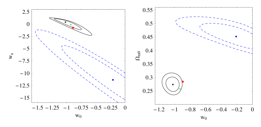
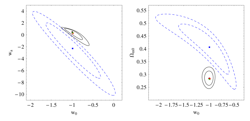
At first, we consider the 397 SNIa Constitution dataset. We fit the CPL model to the observations of SNIa only, SNIa+$A$, SNIa+$R$, and SNIa+$A$+$R$, respectively. The best-fit values are presented in Table 1. In Fig. 1, we also present the $68\%$ and $95\%$ C.L. contours in the $w_{0}-w_{a}$ plane and the $w_{0}-\Omega_{m0}$ plane. From Fig. 1, we find that the Constitution SNIa dataset is in tension (significantly beyond $2\sigma$) with the observations of the CMB and the BAO.

Next, we turn to the 307 SNIa Union dataset. Similarly, we present the results in Table 2 and Fig. 2. From Fig. 2, we can see that the Union dataset is also in tension (beyond $2\sigma$) with the observations of the CMB and the BAO, although the corresponding tension is weaker than the one in the case of Constitution dataset.

Observation	$\chi^{2}_{min}$	$\Omega_{m0}$	$w_{0}$	$w_{a}$
SNIa	461.254	0.453	$-0.207$	$-11.316$
SNIa+$A$	465.438	0.286	$-0.894$	$-0.628$
SNIa+$R$	465.739	0.260	$-0.930$	0.014
SNIa+$A$+$R$	466.1	0.274	$-1.021$	0.413

Table 1: The $\chi^{2}_{min}$ and the best-fit values of $\Omega_{m0}$, $w_{0}$ and $w_{a}$ for the various observations. These results are for the case of Constitution dataset.

Observation	$\chi^{2}_{min}$	$\Omega_{m0}$	$w_{0}$	$w_{a}$
SNIa	310.091	0.451	$-1.013$	$-5.898$
SNIa+$A$	310.915	0.271	$-1.228$	1.502
SNIa+$R$	310.911	0.302	$-1.271$	1.269
SNIa+$A$+$R$	311.154	0.278	$-1.140$	0.859

Table 2: The same as in Table 1, except for the case of Union dataset.

Comparing the cases of the Constitution and Union datasets, we find that they have two common features: (i) the best-fit value of $\Omega_{m0}$ from SNIa data only is fairly larger than $0.3$; (ii) the best-fit value of $w_{a}$ from SNIa data only is strongly negative, namely $w_{a}$ is much smaller than $-1$. On the other hand, they have also two differences: (i) the $\chi^{2}_{min}\sim 460$ is fairly larger than the corresponding degrees of freedom $dof\sim 397$ for the Constitution dataset, whereas the $\chi^{2}_{min}\sim 310$ is approximately equal to the corresponding $dof\sim 307$ for the Union dataset; (ii) for the case of Union dataset, the best-fit value of $w_{0}$ remains about $-1$ for all observations, whereas it is not for the case of Constitution dataset.

Now, one might ask whether or not all SNIa datasets are in tension with the observations of CMB and BAO. A third recent SNIa dataset is the Davis sample r10 , which consists of 192 SNIa. We present the corresponding results in Table 3 and Fig. 3. From Fig. 3, we see that the Davis SNIa dataset is fully consistent with the observations of CMB and BAO. There is no tension in the case of Davis dataset. For the case of 192 SNIa Davis dataset, the corresponding $\chi^{2}_{min}/dof\sim 1$, and its $w_{0}$ remains about $-1$ for all observations, similar to the case of Union dataset. However, its best-fit value of $\Omega_{m0}$ from SNIa data only is much closer to $0.3$ than the cases of Union and Constitution datasets.

Observation	$\chi^{2}_{min}$	$\Omega_{m0}$	$w_{0}$	$w_{a}$
SNIa	195.343	0.349	$-1.105$	$-1.229$
SNIa+$A$	195.453	0.273	$-1.113$	0.526
SNIa+$R$	195.463	0.264	$-1.115$	0.664
SNIa+$A$+$R$	195.485	0.270	$-1.155$	0.818

Table 3: The same as in Table 1, except for the case of Davis dataset.

Figure 2: The same as in Fig. 1, except for the case of Union dataset.

Figure 3: The same as in Fig. 1, except for the case of Davis dataset.

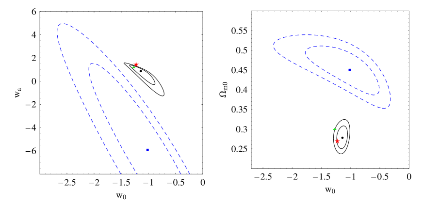
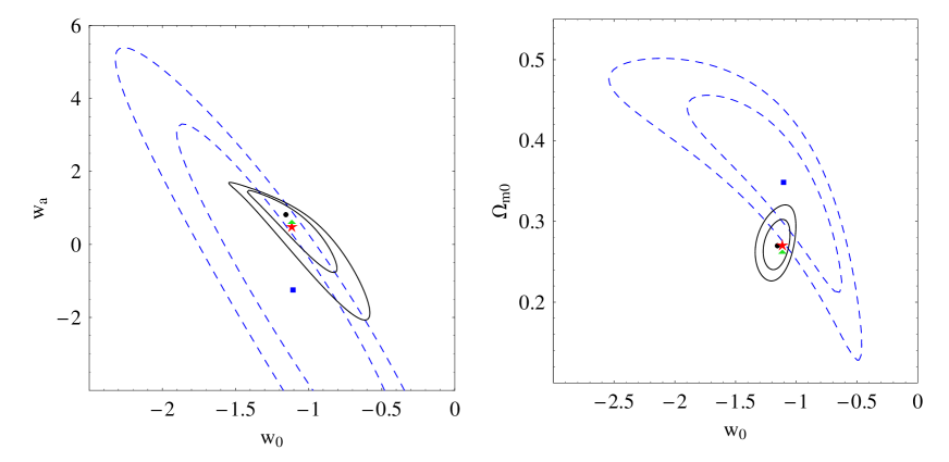
So, the situation is clear now: not all SNIa datasets are in tension with the observations of CMB and BAO. Besides the Davis SNIa dataset shown above, it is well known that the SNLS SNIa dataset is also fully consistent with the observations of CMB and BAO r21 ; r22 . Therefore, the recent SNIa datasets Constitution and Union are in tension not only with the observations of CMB and BAO, but also with the other SNIa datasets such as Davis and SNLS. In fact, they are in the similar situation of the Gold04 and Gold06 SNIa datasets.

UnionOut subset (21 SNIa)
1992bs, 1995ac, 1999bm, 1997o, 2001hu, 1998ba, 04Pat, 05Red, 2002hr, 03D4au,
04D3cp, 03D1fc, 03D4dy, 03D1co, b010, d033, g050, g055, k430, m138, m226
ConstitutionOut subset (34 SNIa)
1992bs, 1992bp, 1995ac, 1999bm, 1996t, 1997o, 1995aq, 2001hu, 1998ba, 04Pat, 05Red,
2002hr, 03D4au, 04D3gt, 04D3cp, 03D4at, 03D1fc, 04D3co, 03D4dy, 04D3oe, 04D1ak,
03D1co, b010, d033, f076, g050, k430, m138, m226, sn01cp, sn02hd, sn03ic, sn07ca, sn07R

Table 4: The names of SNIa in the UnionOut and ConstitutionOut subsets.

IV Outliers with responsibility for the tension

In this section, we elucidate sources of the tension in the Constitution and Union SNIa datasets. Since the Constitution dataset comes from the Union dataset by adding 90 low redshift SNIa from the CfA3 sample, and the tension exists in both Constitution and Union datasets, we speculate that the main sources might be in the Union dataset, and the tension in the Constitution dataset is mainly inherited from the Union dataset. To verify this speculation, we divide the Constitution sample into the high and low redshift groups with the same dividing line $z=0.2$ in r12 ; r11 , and repeat the procedure in the previous section. We find that the results for the high and low redshift groups have only little difference, and this supports our speculation mentioned above. So, we firstly pay our attention to the Union dataset.

In the case of Gold06 SNIa dataset, there are only five subsets (see Table I of r23 ). Using the method of subset truncation (see Sec. V below), the authors of r23 found that the HZSST subset is the main source of the tension in the Gold06 dataset. Then, they isolated six SNIa in the HZSST subset which are mostly responsible for the tension. On the side of Union dataset, there are 13 subsets in it (see Table 3 and Table 11 of r11 ). Even throwing away the first five subsets at low redshift, there are still eight subsets to be considered. By careful observation, we find that three subsets (Barris, Perlmutter, and Riess1998+HZT) are notable, because their RMS listed in Table 3 of r11 are significantly higher than other subsets. Then we try to subtract one of these three subsets in turn, and subtract these three subsets together from the full Union dataset, and see whether or not the tension can be removed. However, we find that it does not work in fact. This leads us to speculate that the main sources of the tension in the Union dataset might be homogeneously distributed in the whole Union dataset, namely, they do not concentrate in a single subset listed in Table 3 of r11 , unlike the case of Gold06 dataset.

Here, we follow the simple method used in r23 to find the outliers responsible for the tension. In r23 , the distance moduli of the six SNIa which are mostly responsible for the tension in Gold06 dataset differ by more than $1.8\sigma$ from the $\Lambda$CDM (with $\Omega_{m0}=0.28$) prediction. Similarly, we firstly fit the flat $\Lambda$CDM model to the whole 307 SNIa in the Union dataset, and find that the best-fit parameter is $\Omega_{m0}=0.287$ (the corresponding $\mu_{0}=\tilde{B}/\tilde{C}=43.16$). Then, we calculate the relative deviation to the best-fit $\Lambda$CDM prediction, $|\mu_{obs}-\mu_{\Lambda CDM}|/\sigma_{obs}$, for all the 307 points. There are 16 SNIa which differ from the best-fit $\Lambda$CDM prediction beyond $2\sigma$. However, we find that the tension cannot be completely removed by subtracting these 16 SNIa from the 307 SNIa Union dataset. We should adopt a severer cut. There are 21 SNIa differing from the best-fit $\Lambda$CDM prediction beyond $1.9\sigma$, and we call them the “UnionOut” subset. The names of these 21 SNIa are listed in Table 4. In Fig. 4, we also plot their distance modulus deviations relative to the best-fit $\Lambda$CDM prediction. These 21 SNIa are indeed homogeneously distributed in the whole Union dataset. On the other hand, their minimum and maximum redshift are $z_{min}=0.0488$ (1995ac) and $z_{max}=1.1900$ (05Red), respectively. It is worth noting that if one chooses to use instead the XCDM model in which $w_{de}=const.$ to find the outliers, the results are almost the same of the case of $\Lambda$CDM model used here.

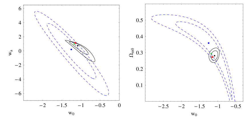
By subtracting the 21 SNIa UnionOut subset from the whole 307 SNIa Union dataset, we obtain the so-called “UnionT” sample (“T” stands for “truncated”). Obviously, the UnionT sample consists of 286 SNIa. Then, we repeat the same fitting as in Sec. III for this 286 SNIa UnionT sample, and present the corresponding results in Table 5 and Fig. 5. From Fig. 5, we clearly see that the UnionT SNIa sample is fully consistent with the other observations, and the tension has been completely removed. On the other hand, by dropping the 21 outliers, the $\chi^{2}_{min}$ significantly reduces from $\chi^{2}_{min}\sim 310$ for the 307 SNIa Union dataset (see Table 2) to $\chi^{2}_{min}\sim 204$ for the 286 SNIa UnionT sample (see Table 5); the corresponding $\chi^{2}_{min}/dof$ has been improved.

Figure 4: $\Delta\mu=\mu_{obs}(z_{i})-\mu_{\Lambda\rm CDM}(z_{i})$ for the SNIa in the UnionOut and ConstitutionOut subsets, where the best-fit $\Lambda$CDM are for the whole Union and Constitution datasets, respectively. See the text for details.

Observation	$\chi^{2}_{min}$	$\Omega_{m0}$	$w_{0}$	$w_{a}$
SNIa	204.060	0.360	$-1.250$	0.242
SNIa+$A$	204.067	0.277	$-1.151$	1.206
SNIa+$R$	204.067	0.298	$-1.181$	1.064
SNIa+$A$+$R$	204.194	0.281	$-1.086$	0.735

Table 5: The same as in Table 1, except for the case of the 286 SNIa UnionT sample.

Notice that since dropping these 21 SNIa from the Union dataset is enough, we need not adopt other severer cuts, such as $1.8\sigma$ or $1.7\sigma$. To preserve the number of usable SNIa as much as possible, the cut $1.9\sigma$ adopted here is the best choice.

Now, let us turn to the Constitution dataset. Similarly, we firstly fit the flat $\Lambda$CDM model to the whole 397 SNIa in the Constitution dataset, and find that the best-fit parameter is $\Omega_{m0}=0.290$ (the corresponding $\mu_{0}=\tilde{B}/\tilde{C}=43.3158$). Then, we calculate the relative deviation to the best-fit $\Lambda$CDM prediction, $|\mu_{obs}-\mu_{\Lambda CDM}|/\sigma_{obs}$, for all the 397 points. We adopt the same cut $1.9\sigma$ used in the Union dataset. There are 34 SNIa differing from the best-fit $\Lambda$CDM prediction beyond $1.9\sigma$, and we call them the “ConstitutionOut” subset. The names of these 34 SNIa are listed in Table 4. In Fig. 4, we also plot their distance modulus deviations relative to the best-fit $\Lambda$CDM prediction. These 34 SNIa are indeed homogeneously distributed in the whole Constitution dataset. On the other hand, their minimum and maximum redshift are $z_{min}=0.015$ (sn07ca) and $z_{max}=1.190$ (05Red), respectively. Obviously, the UnionOut subset and ConstitutionOut subset do heavily overlap. In fact, most SNIa of the ConstitutionOut subset come from the Union sample. Only the last five SNIa in the ConstitutionOut subset come from the CfA3 sample. This confirms our speculation in the beginning of the present section that the tension in the Constitution dataset is mainly inherited from the Union dataset. In other words, the tension is not caused by the low redshift CfA3 sample.

Figure 5: The same as in Fig. 1, except for the case of the 286 SNIa UnionT sample.

By subtracting the 34 SNIa ConstitutionOut subset from the whole 397 SNIa Constitution dataset, we obtain the so-called “ConstitutionT” sample. Obviously, the ConstitutionT sample consists of 363 SNIa. Then, we repeat the same fitting as in Sec. III for this 363 SNIa ConstitutionT sample, and present the corresponding results in Table 6 and Fig. 6. From Fig. 6, we see that the ConstitutionT SNIa sample is consistent with the other observations at the $2\sigma$ level, and the tension has been significantly alleviated, especially comparing Fig. 6 with Fig. 1. On the other hand, by dropping the 34 outliers, the $\chi^{2}_{min}$ significantly reduces from $\chi^{2}_{min}\sim 461$ for the 397 SNIa Constitution dataset (see Table 1) to $\chi^{2}_{min}\sim 269$ for the 363 SNIa ConstitutionT sample (see Table 6); the corresponding $\chi^{2}_{min}/dof$ has been significantly improved.

Notice that if one instead adopt a severer cut $1.8\sigma$ for the case of Constitution dataset, the results are close to the one of $1.9\sigma$ in fact. So, to preserve the number of usable SNIa as much as possible, the cut $1.9\sigma$ adopted here is appropriate.

Observation	$\chi^{2}_{min}$	$\Omega_{m0}$	$w_{0}$	$w_{a}$
SNIa	268.9	0.407	$-0.988$	$-2.270$
SNIa+$A$	269.13	0.286	$-0.983$	0.383
SNIa+$R$	269.134	0.282	$-0.984$	0.438
SNIa+$A$+$R$	269.138	0.284	$-0.996$	0.486

Table 6: The same as in Table 1, except for the case of the 363 SNIa ConstitutionT sample.

Figure 6: The same as in Fig. 1, except for the case of the 363 SNIa ConstitutionT sample.

V Verifying the outliers with the method of random truncation

In the previous section, we have identified the outliers which are mostly responsible for the tension in the Union and Constitution datasets. Here, we will make them more robust by employing the method of random truncation used in r23 .

$q$	$q^{r}$	$\frac{q-\bar{q}^{r}}{\sigma_{q^{r}}}$
$\Omega_{m0}=0.360$	$\Omega_{m0}^{r}=0.448\pm 0.025$	$-3.6\sigma$
$w_{0}=-1.250$	$w_{0}^{r}=-1.028\pm 0.153$	$-1.4\sigma$
$w_{a}=0.242$	$w_{a}^{r}=-5.715\pm 1.902$	$+3.1\sigma$

Table 7: The first column is the best-fit values of the quantity $q$ for the 286 UnionT SNIa sample, which can be read from Table 5. The second column is the mean best-fit value and corresponding $1\sigma$ range of the quantity $q$ for the $N=500$ random truncations. The third column is the relative deviation. See the text for details.

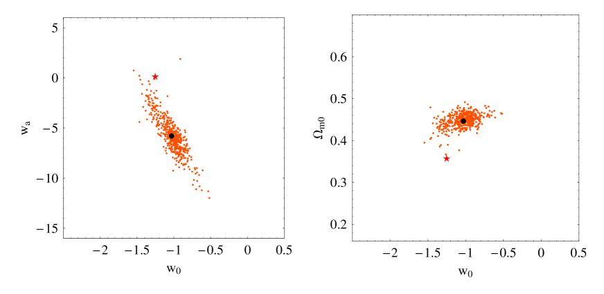
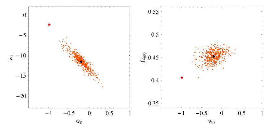
First, we consider the Union SNIa dataset. Following r23 , we compare the best-fit values of $\Omega_{m0}$, $w_{0}$ and $w_{a}$ for the 286 SNIa UnionT data with a large number $N$ of corresponding random truncations of the Union SNIa data (here we adopt the same number $N=500$ as in r23 ). The random truncations involve random subtractions of the same number of SNIa and in the same redshift range as the UnionOut subset from the full Union dataset (notice that $\rm UnionT=Union-UnionOut$). We can easily obtain the mean best-fit value $\bar{q}^{r}$ and the $1\sigma$ range $\sigma_{q^{r}}$ of the quantity $q=\Omega_{m0}$, $w_{0}$ and $w_{a}$ for these random truncations. According to r23 , if the best-fit quantity $q$ of the UnionT sample is within the $1\sigma$ range of the mean best-fit value $\bar{q}^{r}$ of the random truncations, the UnionOut subset is a typical truncation representative of the Union dataset and statistically consistent with it. If on the other hand the best-fit quantity $q$ of the UnionT sample differs from the mean best-fit value $\bar{q}^{r}$ of the random truncations beyond $2\sigma$, we can conclude that the UnionOut subset is not a typical truncation and is systematically different from the full Union dataset r23 . We present the results in Table 7 and Fig. 7. Obviously, the UnionOut subset are systematically different from the full Union dataset, and its 21 SNIa are indeed the outliers. Therefore, it is reasonable to cut these 21 SNIa outliers in the UnionOut subset from the full Union dataset.

Next, we turn to the case of the Constitution dataset. Similarly, we follow the procedure described above (notice that $\rm ConstitutionT=Constitution-ConstitutionOut$), and present the results in Table 8 and Fig. 8. Significantly, the ConstitutionOut subset are systematically different from the full Constitution dataset, and its 34 SNIa are indeed the outliers. Therefore, it is reasonable to cut these 34 SNIa outliers in the ConstitutionOut subset from the full Constitution dataset.

Figure 7: Comparing the best-fit parameters of the 286 UnionT SNIa sample (red stars) with the ones of the 500 random truncations (orange points) in the $w_{0}-w_{a}$ plane and the $w_{0}-\Omega_{m0}$ plane. The mean values of these 500 points are also indicated by the black solid points. See the text for details.

VI Concluding remarks

In the present work, we investigated the tension in the recent SNIa datasets Constitution and Union. We have shown that they are in tension not only with the observations of CMB and BAO, but also with other SNIa datasets such as Davis and SNLS. Then, we found the main sources which are mostly responsible for the tension. Further, we made this more robust by employing the method of random truncation.

Based on the results of this work, we suggest to perform the severer selection cut in the Union and Constitution SNIa datasets to reject the outliers further. While one uses the full 307 SNIa Union dataset and the full 397 SNIa Constitution dataset to constrain the cosmological models, we strongly recommend use also of the 286 SNIa UnionT sample and the 363 SNIa ConstitutionT sample given in this work for comparison. In fact, it is anticipated that the results might be fairly different, and the unusual features which arise from the full 307 SNIa Union dataset and the full 397 SNIa Constitution dataset might disappear in the cases of the 286 SNIa UnionT sample and the 363 SNIa ConstitutionT sample.

As communicated by r35 , the era of precision cosmology has arrived (e.g. r34 and r1 ) and there is a deemed need for an increased understanding of fundamental supernova (SN) physics. In addition, future SN datasets, e.g., those from DES and LSST, will rely significantly on photometric redshift determinations and SN type classifications (particularly in the case of the LSST). The details of SN colors will have to be unraveled if purely photometric SN are to be successfully used for precision cosmology r34 . Enlightened by the results of this work, one might further consider the possible impact of the ConstitutionOut and UnionOut subsets on the understanding of fundamental SN physics and SN colors r35 . We leave this issue as an open question.

$q$	$q^{r}$	$\frac{q-\bar{q}^{r}}{\sigma_{q^{r}}}$
$\Omega_{m0}=0.407$	$\Omega_{m0}^{r}=0.453\pm 0.011$	$-4.0\sigma$
$w_{0}=-0.988$	$w_{0}^{r}=-0.198\pm 0.171$	$-4.6\sigma$
$w_{a}=-2.270$	$w_{a}^{r}=-11.470\pm 1.804$	$+5.1\sigma$

Table 8: The first column is the best-fit values of the quantity $q$ for the 363 ConstitutionT SNIa sample, which can be read from Table 6. The second column is the mean best-fit value and corresponding $1\sigma$ range of the quantity $q$ for the $N=500$ random truncations. The third column is the relative deviation. See the text for details.

Figure 8: Comparing the best-fit parameters of the 363 ConstitutionT SNIa sample (red stars) with the ones of the 500 random truncations (orange points) in the $w_{0}-w_{a}$ plane and the $w_{0}-\Omega_{m0}$ plane. The mean values of these 500 points are also indicated by the black solid points. See the text for details.