Exact encounter times for many random walkers on regular and complex networks

Abstract

The exact mean time between encounters of a given particle in a system consisting of many particles undergoing random walks in discrete time is calculated, on both regular and complex networks. Analytical results are obtained both for independent walkers, where any number of walkers can occupy the same site, and for walkers with an exclusion interaction, when no site can contain more than one walker. These analytical results are then compared with numerical simulations, showing very good agreement.

The last decade has seen an explosion of interest in the properties and applications of complex networks with heterogeneous structure, due to their importance for modelling everything from social systems, such as the internet and networks of acquaintances, to biological ones, such as genetic regulatory networks Albert and Barabási (2002); Newman (2003).

After much initial work on the structure of these networks, attention has now turned to dynamical processes which take place on them, with the aim of understanding the effect that different types of network structure have on the dynamical properties of a system Newman (2003); Barrat et al. (2008). As representative examples in this direction, we mention studies on epidemics Boguñá et al. (2003), the voter model Sood and Redner (2005) and reaction-diffusion processes Colizza et al. (2007) occurring on complex networks.

The properties of random walks on networks have also attracted much attention, both for single walkers Noh and Rieger (2004); Bollt and ben-Avraham (2005); Condamin et al. (2007a) and for multi-walker systems de Moura (2005); Maragakis et al. (2008); Sanders and Larralde (2008). These are perhaps the simplest systems involving motion of particles on networks, and hence are of interest to understand the effect of the network structure on diffusive properties such as mean transit time from one node to another, and the mean time to return to a given node Bollt and ben-Avraham (2005).

These results have applications to individual-based models, in which “agents” (particles with internal states) diffuse in space until they encounter each other, at which point they interact following model-specific rules. If the agents neither die nor reproduce, then one of the key quantities in the system is the time between these encounters, which we call the encounter time.

An example is the Bonabeau model Bonabeau et al. (1995), in which agents represent animals which fight when they meet, with the winner and loser gaining or losing social status. This and similar models Ben-Naim and Redner (2005) undergo a phase transition from a homogeneous, non-differentiated society, to a society with two “social classes”, one successful and one unsuccessful Bonabeau et al. (1995); Okubo and Odagaki (2007); Naumis et al. (2006). One of the key features of the analysis in this model is the timescale given by the mean encounter time Okubo and Odagaki (2007).

Such models can also be studied on complex networks Gallos (2005). Intuitively, for a complex network with highly-connected hubs, all walkers have a tendency to migrate towards the hubs, and thus they will encounter other walkers more frequently. The encounter time provides a quantitative measure of this effect.

Systems of many particles undergoing random walks on complex networks are so complicated that there are usually very few quantities which can be calculated exactly. Nonetheless, in this paper, it is shown that the mean encounter time of a given walker in the system if often amenable to exact calculation.

To calculate such mean encounter times, encounters are viewed in terms of recurrences (or returns) to a set of encounter configurations, and the Kac recurrence theorem is applied. This theorem gives the exact recurrence time to a set in terms of its probability in equilibrium, that is, the probability (frequency) of occupation of a set after the system has evolved for a long time and any transients have died away. For many random walkers on complex networks, even calculating such equilibrium probabilities already requires some work Maragakis et al. (2008). The calculation is also complicated by the necessity to carefully define when encounters occur. By carrying out these steps, we calculate equilibrium probabilities and mean encounter times for many random walkers with and without exclusion on regular and complex networks.

The paper is structured as follows. In sec. I, some notation is introduced, and the main idea used in the paper is presented, namely that encounter times may be expressed as recurrence times. Sections II–IV treat in turn the cases of independent walkers on networks (regular or complex); regular lattices with exclusion; and finally complex networks with exclusion, which is the least tractable case. Section VI gives conclusions.

I Method and notation

We start by establishing some notation and describing the main technique to be used throughout this paper.

I.1 Encounter times and recurrence times

We study a system of $N$ particles undergoing random walks on a finite network. The network consists of $V$ nodes, with edges joining them in a certain structure (see the next subsection). We fix a distinguished walker and assign to it the label “$0$”. The main question treated in this paper is how often this distinguished walker “interacts” with other walkers, that is, what are its encounter times $\tau$. These are defined as the time intervals between the moments at which the distinguished particle meets (encounters) other walkers, measured in terms of steps per particle (a “sweep”).

This random variable $\tau$ has a certain distribution, which in general is quite complicated. In this paper, we consider exclusively its mean $\left\langle\tau\right\rangle$, which we call the mean encounter time of the distinguished walker.

The key idea to calculate mean encounter times is the following: encounters of a given walker correspond exactly to returns, or recurrences, to a particular set, namely the set $E$ of configurations of the $N$ walkers for which an encounter of walker $0$ occurs. A similar method was recently applied in a related context in ref. Sanders and Larralde (2008).

The spatial configuration of walkers is given by $\mathbf{s}:=(s_{1},\ldots,s_{N})$ specifying the location (site) $s_{j}$ of each walker $j$. To describe encounters, however, the spatial locations are not sufficient – we must also specify which walkers are chosen to interact at a given time. The rule for doing so is part of the definition of a given model. We call the combination of the spatial and interaction information an extended configuration.

The mean encounter time $\left\langle\tau\right\rangle$ of walker $0$ is then given exactly by the mean recurrence time $\left\langle\tau^{\text{rec}}_{E}\right\rangle$ to the set $E$ of extended configurations corresponding to that walker’s encounters: $\left\langle\tau\right\rangle=\left\langle\tau^{\text{rec}}_{E}\right\rangle$. We can thus make use of the Kac recurrence theorem Kac (1947, 1959); Condamin et al. (2007b); Aldous and Fill (1999), which gives an exact result for the mean recurrence time $\left\langle\tau^{\text{rec}}_{A}\right\rangle$ to a set $A$ in an ergodic, discrete-time system, namely

$$\left\langle\tau^{\text{rec}}_{A}\right\rangle=\frac{1}{\mathbb{P}_{\mathrm{eq}}\left(A\right)},$$ (1)

where $\mathbb{P}_{\mathrm{eq}}\left(A\right)$ is the probability that the system is in $A$ in equilibrium.

Calculating the mean encounter time thus reduces to the calculation of the equilibrium probability $\mathbb{P}_{\mathrm{eq}}\left(E\right)$ of the encounter set. Note that higher moments and other features of the complete probability distribution of recurrence times are in general much harder to calculate Condamin et al. (2007b); Aldous and Fill (1999), and will not be addressed here.

A special case is that of systems in which the transition probabilities $P_{\mu\to\nu}$ from one configuration, $\mu$, to another, $\nu$, are symmetric, satisfying $P_{\mu\to\nu}=P_{\nu\to\mu}$. The condition of detailed balance, which holds throughout the paper, states that the flux of probability from $\mu$ to $\nu$ in equilibrium is equal to that in the reverse direction:

$$p_{\mu}P_{\mu\to\nu}=p_{\nu}P_{\nu\to\mu}.$$ (2)

Thus, systems with symmetric transition probabilities have equal equilibrium probability for all (accessible) configurations. In this case, the Kac result thus reduces to $\left\langle\tau^{\text{rec}}_{A}\right\rangle=\left|\Omega\right|/\left|A\right|$, where $\Omega$ is the set of all microscopic configurations of the system, and $\left|\cdot\right|$ denotes the cardinality (number of elements) of its argument.

Note that the encounter time as we have defined it above is a single-particle quantity. Since all walkers are equivalent, it may also be calculated by multiplying by $N$ the mean interval between encounters involving any of the walkers in the system.

I.2 Notation for network structure

Throughout the paper, the fixed number of walkers is denoted by $N$, the finite number of nodes in the undirected network by $V$, and the mean density of walkers per node by $\rho:=N/V$. General references for network structure include refs. Albert and Barabási (2002); Newman (2003).

The sites of the network are labelled by $i$, and the degree (number of incident edges) of the site $i$ is denoted by $k_{i}$. The total number of sites in the network with degree $k$ is $n_{k}:=\sum_{i}\delta_{k_{i},k}$, and the degree distribution is then $P(k):=n_{k}/\sum_{k}n_{k}$, which is the probability that a randomly-chosen site has degree $k$.

Finally, $K:=\sum_{i}k_{i}$ denotes the total number of outward edges in the network, which is twice the total number of undirected edges, since each is counted twice, and $\left\langle k\right\rangle:=K/V$ is the mean number of incident edges per site, which satisfies $K=V\left\langle k\right\rangle$ and $N/K=\rho/\left\langle k\right\rangle$.

II Independent walkers on regular and complex networks

The conceputally simplest case is that of many independent random walkers on regular or complex networks, with dynamics given as follows. At each time step, a single one of the $N$ walkers is selected at random (uniformly). If this walker is at site $i$, then it chooses one of its $k_{i}$ neighbouring sites randomly (uniformly), and jumps to it.

Under these dynamics, each walker is independent, and thus the known results for single walkers performing random walks on complex networks can be applied: each walker spends a proportion of time $k_{i}/K$ at node $i$ Noh and Rieger (2004); Aldous and Fill (1999) (i.e., a time proportional to the degree of the node). Recall that $K=\sum_{i}k_{i}$ is the total degree sum.

II.1 Equilibrium distribution

First let us consider the exact equilibrium distribution of the occupation number at a site, i.e., the probability $q_{i}(m)$ of having $m$ particles at a given site $i$ of degree $k_{i}$. Since the walkers are independent, and visit site $i$ with probability $p_{i}=k_{i}/K$, the probability $q_{i}(m)$ that site $i$ has occupation number $m$ is given by the following binomial distribution:

$$q_{i}(m)=\binom{N}{m}\left(\frac{k_{i}}{K}\right)^{m}\left(1-\frac{k_{i}}{K}\right)^{N-m}.$$ (3)

The mean occupation number $\left\langle n_{i}\right\rangle$ of site $i$ is then given by the mean of distribution:

$$\left\langle n_{i}\right\rangle=Np_{i}=\frac{Nk_{i}}{K}=\mu k_{i},$$ (4)

where we have defined $\mu:=\rho/\left\langle k\right\rangle$. Thus $\left\langle n_{i}\right\rangle$ is proportional to $k_{i}$.

In the limit of infinite system size, $V\to\infty$ with $N\to\infty$ but $\rho:=N/V$ fixed, we obtain asymptotically a Poisson distribution:

$$q_{i}(m)\sim\frac{1}{m!}(\mu k_{i})^{m}\exp(-\mu k_{i}),$$ (5)

which is the approximate result obtained in Maragakis et al. (2008).

II.2 Mean encounter time

The mean encounter time of a distinguished walker, labelled by $0$, is calculated using the equilibrium probability $\mathbb{P}_{\mathrm{eq}}\left(E\right)$ of the walker’s encounter set. When there is no exclusion, and several particles may occupy the same site, there are several possible definitions of when encounters occur; here, the following one is chosen. If the walker which moves lands at an unoccupied site, then no encounter occurs. If, however, the walker lands at a site containing $m$ other particles, then the moving walker chooses exactly one of those $m$ particles and interacts with it, i.e., each particle in this pair of walkers undergoes an encounter, but no other particle does so. This allows at most a single encounter at each time step, and forces the encounter to be a result of movement.

Consider the set of encounter configurations defined after the walker has moved, and which contain information about which walker moved and which other walker (if any) is involved in the interaction, apart from the spatial positions of each walker. These encounter configurations are of two types: (i) those in which the distinguished walker was chosen to move, and it moved to a site which already contained at least one walker; and (ii) those in which a walker other than the distinguished one moved, this walker landed on the site which contains the distinguished walker, and furthermore the distinguished walker was chosen as the interaction partner of the moving walker.

In each of these two cases, the probability that the distinguished walker interacts is $1/N$ times the probability that there is at least one other walker on the same site as the distinguished walker after the jump. This is clear in case (i). For case (ii), suppose that there are $m_{i}$ walkers at the site, one of which is the distinguished walker $0$, but that $0$ was not the moving walker. Then one of the other $m_{i}-1$ particles is the one that was chosen to move, with total probability $(m_{i}-1)/N$, and after arriving at the new site an interaction was selected with the distinguished walkers $0$, with probability $1/(m_{i}-1)$. The total probability is the product of these, so we regain the same expression.

It remains to calculate the probability that there is at least one other walker on the same site as the distinguished walker The equilibrium probability that the distinguished particle is on a given site $i$ with a total of $m$ walkers at that site (including the distinguished one) is given by

$$\frac{k_{i}}{K}\binom{N-1}{m-1}\left(\frac{k_{i}}{K}\right)^{m-1}\left(1-\frac{k_{i}}{K}\right)^{(N-1)-(m-1)}.$$ (6)

The term $k_{i}/K$ denotes the probability that the distinguished walker is at site $i$, the second term represents the fact that there are $m-1$ other walkers at the same site, and the last term represents the fact that the remaining $N-m$ walkers are at some other site. The probability that the distinguished particle interacts is given by the previous expression multiplied by $2/N$, provided $m>1$.

The encounter probability if the distinguished particle is at site $i$ can thus be calculated as $2/N$ times the probability that the distinguished particle is not alone at that site:

$$\frac{2k_{i}}{NK}\left[1-\left(1-\frac{k_{i}}{K}\right)^{N-1}\right].$$ (7)

The total encounter probability is then given by a sum over all sites $i$:

$$\mathbb{P}_{\mathrm{eq}}\left(E\right)=\frac{2V}{NK}\sum_{i}k_{i}\left[1-\left(1-\frac{k_{i}}{K}\right)^{N-1}\right],$$ (8)

finally giving the exact result for the mean encounter time per particle:

$$\left\langle\tau\right\rangle=\frac{1}{N\mathbb{P}_{\mathrm{eq}}\left(E\right)}=\frac{\left\langle k\right\rangle}{2\left\langle k\left[1-\left(1-\frac{k}{K}\right)^{N-1}\right]\right\rangle_{k}}.$$ (9)

Here, $\left\langle\cdot\right\rangle_{k}:=\sum_{k}[P(k)\cdot]$ denotes the mean of its argument over the degree distribution. We have divided by $N$ to give the physical time, such that each particle moves on average once per time step. Asymptotically for $N\to\infty$ with $\mu$ fixed, we obtain

$$\left\langle\tau\right\rangle\sim\frac{\left\langle k\right\rangle}{2\left\langle k\left[1-\exp\left(-\mu k\right)\right]\right\rangle_{k}}.$$ (10)

For regular networks with constant coordination number $z$, the degree distribution is $P(k)=\delta(k-z)$. For such networks, we thus obtain

$$\left\langle\tau\right\rangle=\frac{1}{2}\left[1-\left(1-\frac{\rho}{N}\right)^{N-1}\right]^{-1}\sim\frac{1}{2\left[1-\exp(-\rho)\right]},$$ (11)

which is again independent of the coordination number $z$.

III Regular networks with exclusion

We now turn to walkers interacting via an exclusion interaction, so that each site can be occupied by at most one walker de Moura (2005). In this section we consider the dynamics on a regular network, i.e., one in which each site has the same degree (number of neighbours), denoted by $z$. The best-known subclass of such networks consists of regular lattices; other regular networks include small-world networks with a constant number of links per node.

The dynamics are as follows. Initially, the walkers are distributed uniformly on the lattice, but such that there is at most one walker at each site. The dynamics maintain this restriction, as for example in the Bonabeau model discussed in the introduction Bonabeau et al. (1995), and are defined as follows. At each time step, a walker is picked at random. This walker attempts to move to one of its $z$ neighbouring sites, each with equal probability. If the trial site is empty, then the walker moves to the new site. If the trial site is occupied by another walker, however, then the walkers interact, an encounter occurs, and the invading particle remains where it is, without moving.

Since the transition probabilities between two configurations are symmetric, all configurations $\mathbf{s}$ have the same equilibrium probability, $\mathbb{P}_{\mathrm{eq}}\left(\mathbf{s}\right)=1/\left|\Omega\right|=(V-N)!/V!$. More generally, we could allow the two interacting walkers to exchange positions with (fixed) probability $p_{\text{exch}}$. The equilibrium probability $\mathbb{P}_{\mathrm{eq}}\left(\mathbf{s}\right)$, and hence also the mean encounter time $\left\langle\tau\right\rangle$, are unaffected by this.

III.1 Mean encounter time

III.1.1 Mean-field argument for encounter time

The following simple mean-field argument has been used to estimate the mean encounter time in this system, in refs. Bonabeau et al. (1995); Okubo and Odagaki (2007).

At each time step, a single walker moves, each with probability $1/N$, so that the distinguished walker moves on average once every $N$ steps. Suppose that the distinguished walker $0$ does move. The probability of an encounter is the probability that the site it jumps to (one of its $z$ neighbours) is occupied, which is $\rho$, assuming that all walkers are distributed uniformly on the lattice (the mean-field assumption). Similarly, another walker can attempt to move to the site where walker $0$ is sitting. The total probability of the distinguished walker interacting is thus $2\rho$, giving an estimate

$$\left\langle\tau\right\rangle\simeq 1/(2\rho)=V/(2N)$$ (12)

for the mean encounter time per particle. We can refine this calculation by taking $(N-1)/(V-1)$, rather than $\rho$, as the probability that the site jumped to is occupied, by conditioning on the fact that the departure site is occupied. This gives $\left\langle\tau\right\rangle\simeq(V-1)/2(N-1)$. Note that this mean-field calculation is also appropriate for the dynamics without exclusion studied in the last section, in the case of a regular network. Indeed, expanding (11) for small $\rho$ gives back this mean-field result.

The above argument gives an (uncontrolled) approximation of the mean encounter time $\left\langle\tau\right\rangle$ on a lattice. It is not clear, however, how good an approximation it is. We now show that $\left\langle\tau\right\rangle$ can in fact be calculated exactly using the approach of section I. The result of the (refined) mean-field calculation turns out to be exactly correct, suggesting that when we average over all possible configurations of the particles, space “no longer matters”.

III.1.2 Exact calculation of encounter time

For a regular network with exclusion, all microscopic configurations are equally likely, as shown above, so that the Kac recurrence theorem gives $\left\langle\tau\right\rangle=\left|\Omega\right|/\left|E\right|,$ where $E$ again denotes the encounter set of extended configurations for which the distinguished walker $0$ undergoes an encounter.

To calculate the mean encounter time $\left\langle\tau\right\rangle$ of a distinguished walker, we must first explicitly define the set $E$ of encounter configurations. It is not initially clear how to do this, since two walkers can never occupy the same site.

In fact, an encounter occurs exactly when the walker which is chosen to move does so towards an occupied site. To indicate this direction of motion, we augment the positional configuration of the particles $\mathbf{s}$ (before the move) with an arrow which sits on top of the moving walker and points in its chosen direction of motion – one of $z$ possible directions. The extended configurations thus take the form $(\mathbf{s};w,d)$, where $w\in\{1,\ldots,N\}$ is the label of the moving walker and $d\in\{1,\ldots,z\}$ is its chosen direction.

The set $\Omega$ of all extended configurations is thus given by assigning to each of the $N$ walkers a distinct site out of the $V$ possible sites, choosing one of the $N$ occupied sites as the moving walker, and then choosing one of $z$ possible directions of motion. The total number of extended configurations is thus

$$\left|\Omega\right|=\frac{V!}{(V-N)!}Nz.$$ (13)

An encounter involves the distinguished walker $0$ if either (i) walker $0$ is chosen to move, and it attempts to move towards an occupied site; or (ii) walker $0$ occupies the site towards which another walker attempts to move. The first requirement for the set $E$ is thus that the distinguished walker has at least one neighbouring site occupied.

We split the set $E$ of encounter configurations of the distinguished walker into disjoint sets $E_{p}$, in which this walker has exactly $p$ out of its $z$ neighbouring sites occupied (with $1\leq p\leq z$) and it actually does encounter a neighbouring walker, i.e., walker $0$ moves towards an occupied neighbour, or one of the particles in the neighbouring sites jump towards walker $0$. Note that the sets $E_{p}$ do not fill up the whole of $\Omega$, due to these jumping conditions.

The mean encounter time per particle of the distinguished walker $0$ is thus given by

$$\left\langle\tau\right\rangle=\frac{\left|\Omega\right|}{N\left|E\right|}=\frac{\left|\Omega\right|}{N\sum_{p=1}^{z}\left|E_{p}\right|}.$$ (14)

The calculation of the sizes $\left|E_{p}\right|$ of the sets $E_{p}$ proceeds via the following combinatorial arguments.

First consider $E_{1}$, the configurations in which the distinguished walker $0$ has a single occupied site and does encounter its single neighbouring particle when one of them moves. Walker $0$ can be placed in any of the $V$ sites; the single neighbour can then be chosen from the other $(N-1)$ walkers, and placed in any of the $z$ neighbouring sites. The $(N-2)$ remaining walkers can be placed in any of the remaining $(V-(z+1))$ sites. Finally, only two configurations of the arrow are allowed: one which points from the distinguished walker to its single occupied neighbour, and another pointing from the neighbour to the distinguished walker. Thus

$$\left|E_{1}\right|=2zV(N-1)\frac{[V-(z+1)]!}{[V-(z+1)-(N-2)]!}.$$ (15)

Similarly, when the site of the walker $0$ has $p$ occupied neighbours we obtain

$$\left|E_{p}\right|=2pV\binom{z}{p}\frac{(N-1)!}{(N-1-p)!}\frac{[V-(z+1)]!}{[(V-N)-(z-p)]!}.$$ (16)

Here, the binomial coefficient $\binom{z}{p}$ counts the number of ways of choosing the $p$ neighbouring sites out of $z$ to be occupied, the number of permutations $\frac{(N-1)!}{(N-1-p)!}$ gives the number of ways of placing $p$ of the remaining $(N-1)$ walkers in those neighbouring sites, and the arrow can be in any of $2p$ configurations. (These results remain valid for $N$ close to $0$ or close to $V$ if we define the permutations to be $0$ when the number to choose is greater than the number available.)

The expression for $\left|E_{p}\right|$ may be rewritten as

$$\left|E_{p}\right|=2Vz(N-1)!\binom{z-1}{p-1}\binom{V-(z+1)}{N-(p+1)}.$$ (17)

Thus, setting $u:=p-1$, we have

$$\sum_{p=1}^{z}\left|E_{p}\right| =2Vz(N-1)!\sum_{u=0}^{z-1}\binom{z-1}{u}\binom{V-(z+1)}{(N-2)-u}$$ (18)

$$=2Vz(N-1)!\binom{V-2}{N-2}.$$ (19)

The equality in (19) comes from the interpretation of the sum in (18) as the number of ways of choosing $(N-2)$ boxes from a total of $(V-2)$, split into a choice of $u$ from the first $z-1$ boxes, and the remaining $(N-2)-u$ from the $V-(z+1)$ remaining boxes.

Finally, we obtain the exact result

$$\left\langle\tau\right\rangle=\frac{V-1}{2(N-1)}.$$ (20)

Note that this is independent of the coordination number $z$, and hence is valid for any regular network.

One might think that the independence under the dynamics of the Kac result would immediately show that the spatial and mean-field results are the same. In fact, however, the above argument shows that the sets of extended encounter configurations differ in each case, and so the argument is more involved – despite the simplicity of the final result, there does not appear to be a simpler derivation.

III.2 Including a probability of interaction

Within this same framework, we can allow for the possibility that actual encounters occur only a certain fraction $p$ of the time, even if particles meet. This could model a repulsion between agents, so that there is an unwillingess to interact, or a territory that is large enough so that two animals in the same coarse-grained cell move past each other without seeing each other.

To calculate the mean encounter time in this case, the configurations may be extended further, taking the form $(\mathbf{s};w,d,b)$, where the $b$ are independent Boolean variables $b\in\{0,1\}$ which indicate whether or not an encounter occurs.

Denoting the new encounter set by $E^{\prime}:=E\times\{1\}$, where $\{1\}$ denotes when the Boolean variables are true, the result is $\mathbb{P}_{\mathrm{eq}}\left(E^{\prime}\right)=p\mathbb{P}_{\mathrm{eq}}\left(E\right)$, and hence $\left\langle\tau^{\prime}\right\rangle=\frac{1}{p}\left\langle\tau\right\rangle$, so that the effect of including the probability $p$ is an extra factor $\frac{1}{p}$ in the expression for the mean encounter time, as is intuitively expected.

IV Complex networks with exclusion

In this section, we extend the results for many random walkers with an exclusion interaction to the case of complex networks, with heterogeneous degree distribution. The dynamics is as follows. At each step, a walker is selected uniformly. If the walker is at site $i$, then it attempts to jump to one of its $k_{i}$ neighbouring sites, with equal probabilities $1/k_{i}$. If the trial site is unoccupied, then the jump is allowed, and the particle is moved; if the trial site is occupied, then the jump is rejected, and the particle remains where it was.

This case was previously studied in ref. de Moura (2005) by viewing the system as fermions and relating the equilibrium distribution of occupation numbers to the Fermi–Dirac distribution. Here we reconsider these results using a more intuitive method from ref. Maragakis et al. (2008).

The combination of a heterogeneous network and the exclusion interaction makes the calculation of even the equilibrium occupation number distribution highly non-trivial; indeed, it does not appear to be possible to obtain simple, exact results for this quantity in general de Moura (2005). In the next section we show that exact results can be obtained in the case of simple, structured networks. In the following section we then give an approximate argument valid for large networks.

IV.1 Small, structured networks

For complex networks with some structure or which are small enough, it is possible to obtain exact results for the complete equilibrium distribution $\mathbb{P}_{\mathrm{eq}}\left(\mathbf{s}\right)$ for each microscopic configuration $\mathbf{s}$, and from there obtain coarse-grained quantities such as the mean occupation number of a given node, by explicit calculation. Here we give a simple example, which illustrates the general method.

We consider a star-shaped network, representing a single hub in a complex network. The network consists of a central site $0$ with $L$ links to sites $1,\ldots,L$, each of which has only a single link back to the hub. We consider two walkers moving with exclusion on this network, so that the possible configurations $\mathbf{s}$ are of the form $\mathbf{s}=(s_{1},s_{2})$, where $s_{j}$ is the site occupied by particle $j$, although the results are easily extended to more particles. There are two types of configuration: those with a particle at the hub, of the form $\mathbf{s}=(0,i)$ or $(i,0)$, of which there are $2L$; and those with no particle at the hub, of the form $\mathbf{s}=(i,j)$, with $i,j\geq 1$ and $i\neq j$, of which there are $L(L-1)$.

IV.1.1 Equilibrium probability

Let $p:=p_{(i,j)}$ be the equilibrium probability to be in configuration $(i,j)$, with $i\neq 0$ and $j\neq 0$, i.e., with no particles at the hub). All probabilities are symmetric in the two arguments. The transition probabilities are given by

$$P\left[(0,i)\to(j,i)\right]=\frac{1}{2L};\qquad P\left[(j,i)\to(0,i)\right]=\frac{1}{2}.$$ (21)

The second equation follows from the fact that there is a probability $1/2$ to move each particle from a configuration $(j,i)$, to arrive at the configuration $(0,i)$ or $(j,0)$. From $(j,0)$, with probability $1/2$ the particle at site $j$ is chosen, but it is unable to move due to the exclusion interaction and the presence of the other particle at the hub $0$, which is the only site available. If the particle at the hub is chosen, then it moves to site $i\neq j$ with probability $1/L$.

The detailed balance condition

$$p_{(0,i)}P\left[(0,i)\to(j,i)\right]=p_{(j,i)}P\left[(j,i)\to(0,i)\right]$$ (22)

then shows that $p_{(0,i)}=Lp$. Since the normalisation condition $\sum_{\mathbf{s}}\mathbb{P}_{\mathrm{eq}}\left(\mathbf{s}\right)=1$ must be satisfied, we have

$$2L^{2}p+L(L-1)p=1,$$ (23)

and hence $p=1/(3L^{2}-L)$.

We have thus found the equilibrium probability $\mathbb{P}_{\mathrm{eq}}\left(\mathbf{s}\right)$ of each configuration $\mathbf{s}$. To find the mean occupation number $\left\langle n_{i}\right\rangle$ of site $i$, we must sum over configurations:

$$\left\langle n_{i}\right\rangle=\sum_{\mathbf{s}}n_{i}(\mathbf{s})\mathbb{P}_{\mathrm{eq}}\left(\mathbf{s}\right),$$ (24)

where $n_{i}(\mathbf{s})$ is the occupation number of site $i$ in the configuration $\mathbf{s}$. In the case of exclusion, $n_{i}$ can only take the values $0$ and $1$, so that the mean occupation of the hub is given by a sum over those configurations $\mathbf{s}$ which have a particle in the hub, giving

$$\left\langle n_{0}\right\rangle=2L^{2}p.$$ (25)

The mean occupation of a site $i\neq 0$ is similarly given by a weighted sum over those configurations which have a particle in site $i$:

$$\left\langle n_{i}\right\rangle =p_{(i,0)}+p_{(0,i)}+\sum_{j=1,\ldots,L;j\neq i}\left[p_{(i,j)}+p_{(j,i)}\right]$$ (26)

$$=2Lp+2(L-1)p=(4L-2)p.$$ (27)

The normalisation $\left\langle n_{0}\right\rangle+\sum_{i=1}^{L}\left\langle n_{i}\right\rangle=2$ is then correctly satisfied, and we have also checked these exact results with numerical simulations (not shown).

In such structured networks, we can also proceed to obtain results for more detailed features of the probability distributions, such as higher moments.

IV.1.2 Mean encounter time

Identifying particle $1$ as the distinguished walker, the probability $\mathbb{P}_{\mathrm{eq}}\left(E\right)$ of its encounter set may be calculated in a similar way to that in sec. III.1, as the sum over all configurations such that $1$ has a neighbour, weighted by the probability that an encounter occurs, i.e., that $1$ interacts with the neighbour. In this simple system, encounters can occur only with configurations of the form $(0,i)$ or $(i,0)$, for which one of the particles is at the hub. In this case, the probability that the two particles interact is $1/2+1/(2L)$, since the particle not at the hub always tries to jump towards the hub, whereas the particle at the hub usually jumps towards an empty node.

$$\mathbb{P}_{\mathrm{eq}}\left(E\right) =\sum_{i}\left[p_{(i,0)}+p_{(0,i)}\right]\left[\frac{1}{2}+\frac{1}{2L}\right]$$ (28)

$$=p(L^{2}+L),$$ (29)

giving

$$\left\langle\tau\right\rangle=\frac{1}{p(L^{2}+L)}=3-\frac{4}{L+1}.$$ (30)

For a network with exclusion, the total number of spatial configurations is $V!/(V-N)!$, so that for arbitrary networks this kind of calculation becomes intractable. Nonetheless, for networks which are small and/or have enough structure it can be carried out relatively easily.

IV.2 Equilibrium distribution in the large-system approximation

For systems with many nodes, for which the above direct method is impractical, it is instead necessary to turn to an approximation in which we assume that the occupation numbers of neighbouring sites are independent Maragakis et al. (2008); de Moura (2005). This is valid when the system is large, or in a grand-canonical situation, where the number of particles in the system can fluctuate about a mean value, since in a finite system with a fixed number of particles, the presence or absence of a particle at a site $i$ affects the conditional probability to have a particle at site $j\neq i$, given the occupation number of site $i$.

To derive the equilibrium distribution in this approximation, the method of ref. Maragakis et al. (2008) can be applied. As shown below, the results which were first obtained in ref. de Moura (2005) are recovered, in a more direct way.

IV.2.1 Neighbouring sites

Let $p_{i}$ be the probability that site $i$ is occupied in equilibrium. Due to the exclusion interaction, the occupation number $n_{i}$ of site $i$ is either $0$ or $1$, so that its mean is $\left\langle n_{i}\right\rangle=p_{i}$. Thus $\sum_{i}p_{i}=N$, the total number of particles present in the system.

Suppose that the particle on site $i$ is chosen to move towards a neighbouring site $j$. The probability that the trial site is unoccupied is $(1-p_{j})$ under the independence approximation, and the probability that the direction towards site $j$ is chosen is $1/k_{i}$. We thus obtain $P_{i\to j}=\frac{1}{Nk_{i}}(1-p_{j})$.

Here the assumption of independence of occupation states has already been used.

In equilibrium, the detailed balance condition $p_{i}P_{i\to j}=p_{j}P_{j\to i}$ gives

$$\frac{1}{k_{i}}p_{i}(1-p_{j})=\frac{1}{k_{j}}p_{j}(1-p_{i}).$$ (31)

Rearranging to collect all terms in $p_{i}$ and $p_{j}$ on opposite sides of the equation we see that

$$\frac{p_{i}}{k_{i}(1-p_{i})}=\frac{p_{j}}{k_{j}(1-p_{j})},$$ (32)

and hence

$$\frac{p_{i}}{k_{i}(1-p_{i})}=C,$$ (33)

where $C$ is a site-independent constant. Finally we obtain

$$p_{i}=\frac{Ck_{i}}{1+Ck_{i}}=\frac{1}{1+Ak_{i}^{-1}},$$ (34)

where $A$ is another constant, as was found in ref. de Moura (2005). The constant $A$ is determined by the normalisation condition $\sum p_{i}=N$, and thus depends on the entire set of degrees $\{k_{i}\}$.

IV.2.2 Single site

A single-site variant of the above Markov chain method gives an alternative derivation. Consider a site $i$ with degree $k_{i}$. Let $p_{0}^{(i)}=1-p_{i}$ and $p_{1}^{(i)}=p_{i}$ be the equilibrium probability that the site is empty or occupied, respectively. We first need a mean-field type estimate of the transition probabilities from empty to occupied, $P_{0\to 1}^{(i)}$, and vice versa, $P_{1\to 0}^{(i)}$.

Due to the way the network is constructed, following a given link from a given node leads to a new node $j$ with probability $k_{j}/K$ which depends on $j$, since node $j$ has $k_{j}$ incoming edges de Moura (2005). The particle at node $j$ then jumps to site $i$ with probability $1/k_{j}$, giving Maragakis et al. (2008)

$$P_{0\to 1}^{(i)} =\frac{1}{N}\sum_{j}\frac{k_{j}}{K}p_{j}\frac{1}{k_{j}}=\frac{1}{N}k_{i}\frac{\rho}{\left\langle k\right\rangle},$$ (35)

The second equality follows since $\sum_{j}p_{j}=N$ and $N/K=\rho/\left\langle k\right\rangle$.

We calculate $P_{1\to 0}^{(i)}$ by arguing similarly. If the particle at site $i$ is selected, with probability $1/N$, then it can attempt to move to any of the $k_{i}$ neighbours, each with probability $1/k_{i}$. The neighbour is site $j$ with probability $k_{j}/K$. The move is successful only if the neighbour is empty, due to the exclusion, and occurs with probability $1-p_{j}$, giving

$$P_{1\to 0}^{(i)}=\frac{1}{N}\sum_{j}\frac{k_{j}}{K}(1-p_{j}).$$ (36)

Note the extra factor $(1-p_{j})$ compared to the expression for independent dynamics in ref. Maragakis et al. (2008).

Detailed balance gives $(1-p_{i})P_{0\to 1}^{(i)}=p_{i}P_{1\to 0}^{(i)}$, from which we finally obtain (34) again, but now with an expression for $A$:

$$A=\frac{\left\langle k\right\rangle}{\rho}\left(1-\frac{\sum_{j}k_{j}p_{j}}{K}\right)=\frac{1}{N}\sum_{j}k_{j}(1-p_{j}).$$ (37)

Although this equation appears to give new information, in fact it turns out to be equivalent to the normalisation condition.

Unfortunately, it does not seem to be possible to solve this equation exactly to find $A$ and the $p_{i}$ explicitly. In ref. de Moura (2005), $A$ was found numerically by solving the normalisation equation $\sum_{j}p_{j}=N$. This gives no insight into the quantity $A$, however.

An alternative is to find approximations to $A$. A first approximation is obtained by taking all $k_{i}$ equal to $\left\langle k\right\rangle$ in (37), giving

$$A^{(0)}=\frac{1-\rho}{\rho}\left\langle k\right\rangle.$$ (38)

As shown below in fig. 2, this already gives a reasonable approximation to the distribution $p_{i}$ for networks for which the deviation of the $k_{i}$ from their mean is small, although the corresponding $p_{i}^{(0)}$ calculated using this value for $A$ do not satisfy the normalisation condition.

Further approximations may be obtained – either analytically or numerically – by an iterative scheme based on (37) and with the initial value (38) for $A$:

$$A^{(n+1)} :=\frac{1}{N}\sum_{j}k_{j}(1-p_{j}^{(n)});$$ (39)

$$p_{i}^{(n)} :=\frac{1}{1+A^{(n)}k_{i}^{-1}},$$ (40)

giving

$$A^{(n+1)}=\frac{1}{N}\sum_{j}\frac{1}{[A^{(n)}]^{-1}+k_{j}^{-1}}.$$ (41)

This iteration, which is easily implemented computationally, quickly converges to a fixed point which gives the numerically exact value of $A$ and of the $p_{j}$ for the given degree sequence, and thus provides an alternative numerical method to that used in ref. de Moura (2005).

IV.3 Mean encounter time in the large-system approximation

The calculation of the mean encounter time in the large-system approximation, supposing that the occupation probabilities of neighbouring sites are independent of each other, proceeds as follows..

For the distinguished walker $0$ to have an encounter, it first must be at some site $i$, which occurs with probability $p_{i}/N$ (giving a total probability $1$ to be at some site). There are two possibilities for such encounters: either walker $0$ is chosen to jump, in which case it has an encounter if the trial site is occupied, or another walker attempts to jump onto the site occupied by walker $0$.

The probabilities for these two possibilities are calculated in the same way as the transition probabilities in the previous section. Again denoting by $E$ the encounter set of the distinguished walker, we obtain

$$\mathbb{P}_{\mathrm{eq}}\left(E\right)=\sum_{i}\frac{p_{i}}{N}\left[\sum_{j}\frac{k_{j}}{K}p_{j}+k_{i}\sum_{j}\frac{k_{j}}{K}p_{j}\frac{1}{k_{j}}\right]=\frac{2}{K}\sum_{j}k_{j}p_{j},$$ (42)

and hence

$$\left\langle\tau\right\rangle=\frac{V\left\langle k\right\rangle}{2\sum_{j}k_{j}p_{j}}.$$ (43)

We remark that this calculation is basically that of the jamming probability studied in ref. de Moura (2005), i.e., the probability that the particle which attempts to move is jammed (blocked) de Moura (2005) – that is, that an encounter occurs.

V Numerical results

In this section, the analytical results obtained in previous sections are compared with the results of numerical simulations on two different types of network, one regular and one complex.

V.1 Regular network: linear chain

First consider a regular network, consisting of a linear chain of $V=100$ sites, where each site is connected to its two nearest neighbours, with periodic boundary conditions.

The mean encounter time of a distinguished walker for dynamics both with and without exclusion on this chain are shown in fig. 1 as a function of the total number of walkers, $N$, between $2$ and $V$. To distinguish the two cases, the time is shown as $N\left\langle\tau\right\rangle$, i.e., as a raw number of steps, rather than as a number of sweeps. The analytical and numerical results in both cases agree very well.

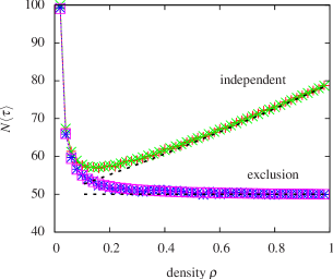
Figure 1: Mean encounter time $N\left\langle\tau\right\rangle$ on a linear chain of length $V=100$, as a function of the number of particles $N$, with and without exclusion. Numerical results, evaluated as a mean over $10^{8}$ steps, are compared to the analytical results; lines are shown as a guide for the eye. Error bars are of the order of the symbol size. There is excellent agreement in both cases. Dashed lines show the asymptotic behaviour.

The figure shows that the mean encounter time (in sweeps) depends very little on the dynamics. The mean encounter time in the case of exclusion dynamics is generally slightly shorter, which we can attribute to the fact that the particles must be spread out more uniformly through the system in this case due to the exclusion interaction.

Note that at first glance the Kac result (20) does not hold for a one-dimensional dynamics with strict exclusion, since this result assumes ergodicity, i.e., that it any configuration can be reached from any other, which is not the case due to the one-dimensional nature of the system: each walker is always confined between the same two neighbours. However, the result is in fact valid. This is because the mean encounter time is a single-particle quantity, which can be calculated by averaging over all particles in the system. The result for the global encounter time (taking into account encounters of any particle) will be the same in the ergodic and non-ergodic cases, since each time between two encounters is unaffected, but may be assigned to a different walker. This then implies equality also for the encounter times of a distinguished walker.

V.2 Complex networks: random graphs with power-law degree distributions

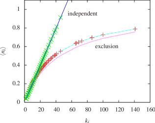
Figure 2: Mean occupation number $\left\langle n_{i}\right\rangle$ for each site $i$, as a function of the degree $k_{i}$ of the site, for dynamics with and without exclusion, on a single random network with power-law degree distribution $P(k)\sim k^{-\alpha}$ with $\alpha=2.5$. The network has $V=1000$ nodes and mean degree $\left\langle k\right\rangle=5.036$. The numerical data for each site is shown as a symbol, and the curves show the analytical results; the lowest curve is the zeroth-order approximation $p_{i}{(0)}$ in the exclusion case. The complete curve in the case of independent dynamics continues to grow linearly for larger $k_{i}$ (not shown).

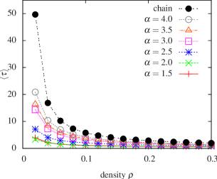
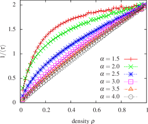
Figure 3: (a) Mean encounter time $\left\langle\tau\right\rangle$ of a distinguished walker on networks with power-law degree distribution $P(k)\sim k^{-\alpha}$, for different values of $\alpha$ with $V=1000$ sites and for a chain with $V=100$, as a function of the density, $\rho$. Only data for exclusion dynamics are shown; data for independent walkers are very close to these. To highlight the differences between the curves, (b) shows $1/\left\langle\tau\right\rangle$ for different $\alpha$ compared to the analytical results, drawn with black dotted lines. The lowest dashed line shows the mean-field result for comparison.

The second case is that of random networks with a power-law degree distribution $P(k)\sim k^{-\alpha}$. These are generated according to the prescription in ref. Newman et al. (2001): (i) a degree sequence $(k_{i})_{i=1}^{V}$ is generated from the distribution, rejecting each $k_{i}$ if it does not satisfy $2\leq k_{i}\leq N$; (ii) $k_{i}$ “stubs” are generated at each node $i$; and (iii) pairs of stubs are chosen at random to be connected. This method gives networks which in general include self-links from a given node back to itself, as well as multiple links between nodes Catanzaro et al. (2005). Since both the random-walk dynamics and our analytical results take these into account, no attempt was made to remove them from the network, as is done in ref. Catanzaro et al. (2005) for example; rather, this gives a more stringent test of the analytical results. The imposed minimum degree of $2$ at each node ensures that the resulting network is connected with probability one Catanzaro et al. (2005).

Power-law networks with smaller values of $\alpha$ have more nodes of high degree, and in particular a few very highly-connected hubs. Particles will concentrate at or near these hubs, and so intuitively this will lead to shorter mean encounter times. For an infinite system, the degree distribution has a well-defined mean if and only if $\alpha>2$, but for a finite network we can also consider $\alpha<2$. We do, however, impose the total number of sites as a cutoff for the maximum allowed degree.

Figure 2 shows a comparison of numerical and analytical results for the mean occupation number $\left\langle n_{i}\right\rangle$ (which is equal to $p_{i}$ in the case of exclusion dynamics) in the case $\alpha=2.5$, for dynamics with and without exclusion. We see that the zeroth-order approximation $p_{i}{(0)}$ already provides a good approximation for exclusion dynamics, even though the values of $k_{i}$ cover a wide range of values, including far from the mean $\left\langle k\right\rangle$. The converged $p_{i}$ agree very well indeed with the numerical values, as was already found in ref. de Moura (2005).

Figure 3 shows the mean encounter times for networks with different power-law degree distributions. Part (a) shows $\left\langle\tau\right\rangle$, and part (b) shows $1/\left\langle\tau\right\rangle$ to exhibit more clearly the differences between networks with different $\alpha$. The main observation is that networks with smaller $\alpha$, i.e., with highly-connected hubs, indeed have lower mean encounter times. This is highlighted in 4, where the encounter time is plotted for different values of $\rho$ as a function of $\alpha$. We also see that the exact and numerical results again agree very well. Results for non-exclusion dynamics on the same graphs are very similar, although slightly larger, for the same reason as in regular networks, and are not shown.

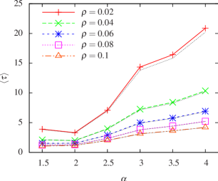
Figure 4: Mean encounter time $\left\langle\tau\right\rangle$ as a function of the power-law exponent $\alpha$, for different densities $\rho$, on networks of size $V=1000$. The black dotted lines show the analytical results for comparison.

VI Conclusions

In conclusion, this paper has shown that it is often possible to calculate analytically a key quantity in systems consisting of many interacting random walkers, namely the mean encounter time of a given particle. This was carried out for the case of independent walkers and for walkers with exclusion on regular and complex networks, and the results were successfully compared to numerical simulations.

For a given graph, the mean encounter time is very similar whether dynamics with or without exclusion is used, even though the mean occupation numbers can be quite different. This could change with a different choice of interaction rule in the case of independent walkers.

At first glance, it seems that the results require averages over a very long time to be valid, namely the time required for a given walker to explore the whole system. In the case of a high-density system with exclusion, for example, this timescale could be very long. In fact, however, the results are unaffected by considering interacting particles which exchange positions, so that the timescale required is more like that for a single particle to explore the system when no others are present.

The method employed can be extended to other mean encounter times of interest. For example, interaction times between two distinguished walkers can be found. The extension of these results to higher moments and the full probability distribution of encounter times, and the effect of different network structures on those results, are subjects for future study.

The author thanks G. Naumis for suggesting to study the Bonabeau model, M. Aldana for a helpful conversation, and H. Larralde for useful discussions and for a reading the manuscript critically. Financial support from the PROFIP program of DGAPA-UNAM is acknowledged.

Appendix A Intuitive derivation of the Kac recurrence theorem

Rigorous derivations of the Kac recurrence theorem, such as can be found in refs. Kac (1947, 1959); Condamin et al. (2007b), do not always provide intuition about why the result should be true. Here, a simple, non-rigorous argument is given which captures the essence of the result.

To find the mean recurrence time $\left\langle\tau^{\text{rec}}_{A}\right\rangle$ to a set $A$ in a discrete-time, ergodic system, consider a long trajectory of the system, of length $T$ time steps. If at time $t$ the system is in $A$, then write a $1$; if it is outside $A$, then write a $0$, thus coding the trajectory as a symbol sequence of $0$s and $1$s.

At long times, $T\to\infty$, the proportion of $1$s in the sequence converges to the equilibrium probability $\mathbb{P}_{\mathrm{eq}}\left(A\right)$ that the system is inside $A$. This is the crucial part of the argument. From a physical point of view, it is a weak version of the Boltzmann ergodic hypothesis, but in the case of discrete-time stochastic processes it is made rigorous by the Kac recurrence theorem Kac (1947). The number of $1$s occurring in time $T$ is thus roughly $T\mathbb{P}_{\mathrm{eq}}\left(A\right)$. Similarly, the total time spent outside $A$ is approximately $T\left[1-\mathbb{P}_{\mathrm{eq}}\left(A\right)\right]$.

Now consider rearranging the list of $1$s and $0$s so that approximately the same number of $0$s occurs between each pair of consecutive $1$s. The mean recurrence time is then this number of $0$s, plus $1$ for the extra step to return to the next $1$, giving

$$\left\langle\tau^{\text{rec}}_{A}\right\rangle=1+\frac{T\left[1-\mathbb{P}_{\mathrm{eq}}\left(A\right)\right]}{T\,\mathbb{P}_{\mathrm{eq}}\left(A\right)}=\frac{1}{\mathbb{P}_{\mathrm{eq}}\left(A\right)},$$ (44)

which is the Kac result.

References

- Albert and Barabási (2002) R. Albert and A. Barabási, Rev. Mod. Phys. 74, 47 (2002).
- Newman (2003) M. E. J. Newman, SIAM Review 45, 167 (2003).
- Barrat et al. (2008) A. Barrat, M. Barthélemy, and A. Vespignani, Dynamical Processes on Complex Networks (Cambridge University Press, 2008).
- Boguñá et al. (2003) M. Boguñá, R. Pastor-Satorras, and A. Vespignani, Phys. Rev. Lett. 90, 028701 (2003).
- Sood and Redner (2005) V. Sood and S. Redner, Phys. Rev. Lett. 94, 178701 (2005).
- Colizza et al. (2007) V. Colizza, R. Pastor-Satorras, and A. Vespignani, Nature Phys. 3, 276 (2007).
- Noh and Rieger (2004) J. D. Noh and H. Rieger, Phys. Rev. Lett. 92, 118701 (2004).
- Condamin et al. (2007a) S. Condamin, O. Benichou, V. Tejedor, R. Voituriez, and J. Klafter, Nature 450, 77 (2007a).
- Bollt and ben-Avraham (2005) E. M. Bollt and D. ben-Avraham, New J. Phys. 7, 26 (2005).
- de Moura (2005) A. P. S. de Moura, Phys. Rev. E 71, 066114 (2005).
- Maragakis et al. (2008) M. Maragakis, S. Carmi, D. ben-Avraham, S. Havlin, and P. Argyrakis, Phys. Rev. E 77, 020103 (2008).
- Sanders and Larralde (2008) D. P. Sanders and H. Larralde, Europhys. Lett. 82, 40005 (2008).
- Bonabeau et al. (1995) E. Bonabeau, G. Theraulaz, and J. Deneubourg, Physica A 217, 373 (1995).
- Ben-Naim and Redner (2005) E. Ben-Naim and S. Redner, J. Stat. Mech. 2005, L11002 (2005).
- Okubo and Odagaki (2007) T. Okubo and T. Odagaki, Phys. Rev. E 76, 036105 (2007).
- Naumis et al. (2006) G. Naumis, M. del Castillo-Mussot, L. Pérez, and G. Vázquez, Physica A 369, 789 (2006).
- Gallos (2005) L. K. Gallos, Int. J. Mod. Phys. C 16, 1329 (2005).
- Kac (1947) M. Kac, Bull. Amer. Math. Soc. 53, 1002 (1947).
- Kac (1959) M. Kac, Probability and Related Topics in Physical Sciences (American Mathematical Society, 1959).
- Condamin et al. (2007b) S. Condamin, O. Bénichou, and M. Moreau, Phys. Rev. E 75, 021111 (2007b).
- Aldous and Fill (1999) D. Aldous and J. A. Fill, Reversible Markov Chains and Random Walks on Graphs (1999), available online at http://www.stat.berkeley.edu/~aldous/RWG/book.html.
- Newman et al. (2001) M. E. J. Newman, S. H. Strogatz, and D. J. Watts, Phys. Rev. E 64, 026118 (2001).
- Catanzaro et al. (2005) M. Catanzaro, M. Boguñá, and R. Pastor-Satorras, Phys. Rev. E 71, 027103 (2005).