Twirling motion of actin filaments in gliding assays with non-processive myosin motors

Abstract

We present a model study of gliding assays in which actin filaments are moved by non-processive myosin motors. We show that even if the power stroke of the motor protein has no lateral component, the filaments will rotate around their axis while moving over the surface. Notably, the handedness of this twirling motion is opposite from that of the actin filament structure. It stems from the fact that the gliding actin filament has “target zones” where its subunits point towards the surface and are therefore more accessible for myosin heads. Each myosin head has a higher binding probability before it reaches the center of the target zone than afterwards, which results in a left-handed twirling. We present a stochastic simulation and an approximative analytical solution. The calculated pitch of the twirling motion depends on the filament velocity (ATP concentration). It reaches about 400nm for low speeds and increases with higher speeds.

Introduction

Gliding assays, also known as motility assays, represent the oldest in vitro technique to study motor proteins toyoshima87 ; howard89 . They consist of attaching motors (like myosins or kinesins) with their tails to a glass surface and adding the filaments (actin or microtubules). The motors will then pull the filaments and make them glide over the surface (Fig. 1A). Gliding assays are the most convenient way of testing motors for their functionality, measuring their speed in the absence of load and for testing their processivity. Several experimental and theoretical studies were dealing with the pathways of such filaments in the two-dimensional plane duke95 ; bourdieu95 ; Gibbons.Jose2001 . Interestingly, one group observed that gliding actin filaments move in a helical fashion Tanaka.Ishiwata1992 ; nishizaka93 . In a subsequent experiment the pitch of rotation was determined as about $1\,\rm\mu m$, although the applied optical detection method did not allow discrimination between left- and right-handed rotation Sase.Kinosita1997 .

Helical motion of myosin motors has been very important in a somewhat different context. The processive motor myosin V has an average step size that is close, but not precisely equal to the actin periodicity. The helical motion of a motor around the actin filament therefore presents a very accurate way of measuring the difference between its step size and the filament pitch. Ali and coworkers have observed that myosin V walks on an actin filament along a left-handed helix with a pitch of $2.2\,\rm\mu m$ Ali.Ishiwata2002 and thus has a step size slightly shorter than the actin half-pitch (for a discussion of the myosin V step size see Vilfan2005 ; vilfan2005b ).

Myosin VI, despite having a shorter lever arm than myosin V, showed either straight walking, or, in $20\%$ of cases, a helical path with a pitch of $2.3\,\rm\mu m$ Ali.Ikebe2004 . Sun et al. Sun.Goldman2007 confirmed this result, but also showed that the relatively straight motion contains a large amount of random wiggling. New experiments on myosin X also show a left-handed helical motion with a pitch that is somewhat shorter than that of myosin V and VI Arsenault.Goldman2009 .

In a recent experimental study Beausang and coworkers Beausang.Goldman2008 used polarized total internal reflection microscopy to study the twirling motion of actin filaments in gliding assays with processive myosin V and non-processive muscle myosin (myosin II). While the twirling of filaments driven by myosin V agreed with the helical movement of single molecules mentioned above, myosin II interestingly showed a left-handed twirling motion as well. This result came as a surprise and the left-handed rotation is opposite from the observations by Nishizaka et al. nishizaka93 . But they are not in direct contradiction, as they were obtained with quite different ATP concentrations.

While the pitch of the twirling motion is a direct measure for the step size of processive motors, its interpretation is more complicated with non-processive ones. They could clearly generate twirling motion if there was a lateral component of the power stroke. In fact, there exists indirect evidence for such an asymmetry in myosin V Purcell.Spudich2005 . However, we will show in this paper that there is another, more subtle, effect that can cause twirling motion of actin filaments in a gliding assay, even if the myosin heads exhibit no lateral motion. This effect stems from the fact that myosin heads can only bind to an actin filament in so called target zones, where the actin binding sites have approximately the right orientation (Fig. 1D) Steffen.Sleep2001 ; Capitanio.Bottinelli2006 . When a target zone is approaching a myosin head, the latter is more likely to bind at the beginning of the target zone than at its end, because it is more likely that it is already bound by that time. In this paper we will show simulation results and develop an approximative theory to estimate the pitch of helical motion resulting from this effect. Of course, we cannot exclude that there are other contributions towards the helicity. But, because the rotation is relatively weak as compared with the longitudinal motion, these effects can easily be treated separately and the total rotation is simply their superposition.

(A)

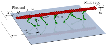
(B)

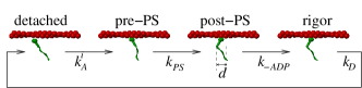
(C)

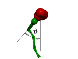
(D)

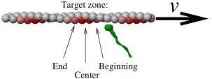
Figure 1: (A) Model definition. The linear motion and rotation of the actin filament are denoted with $X$ and $\Theta$. Motors are situated underneath the actin filament at randomly distributed positions $x_{M}^{j}$ and each motor can be in the detached, pre-powerstroke or post-powerstroke state. (B) Duty cycle of a myosin head. The head binds to the actin site $i$ with rate $k_{A}^{i}$, then quickly undergoes the power stroke with rate $k_{PS}$, releases ADP with rate $k_{-ADP}$ and detaches with rate $k_{D}$. The step size is $d=8\,\rm nm$. (C) Front view of a bound head. For the sake of simplicity, we assume that the azimuthal component of the elastic energy needed to bind to site $i$ only depends on the angle $\vartheta$. (D) Target zones on an actin filament. When a filament is moving past an actin head, it is more likely to bind to submits pointing towards the myosin-covered surface. Red color denotes the sites with the highest binding rate. Besides that, sites at the beginning of a target zone have a higher binding probability than those at its end.

Model definition

In order to concentrate on the effect of filament rotation, we define a model with simplified myosin kinetics, essentially containing a detached state, a bound pre-powerstroke state, a bound post-powerstroke state with ADP and a bound rigor state. At the same time, we take into account the full helical structure of the actin filament. We propose an actin filament which can move in one direction and rotate around its axis. The position of the actin filament at a given time is therefore described with the coordinates $(X,\Theta)$. As follows from the helical structure of the actin filament, the $x$-coordinate of each bindings site is $X+ia$ and its azimuth angle $\Theta+i\vartheta_{0}$, where $\vartheta_{0}=-(13/28)\times 360^{\circ}=-167.14^{\circ}$ is the rotation and $a=2.75\,\rm nm$ the axial rise per subunit. The definition of the model is illustrated in Fig. 1.

We assume that the myosin motors are distributed randomly directly under the gliding actin filament (a discussion how this simplified, one-dimensional model follows from the full, 2-D model is given in the Appendix). The motor numbered $j$ is anchored at position $x_{M}^{j}$. The elastic energy cost of binding a head to the site $i$ consists of a longitudinal component with stiffness $K$ and and an angular component with stiffness $K_{\vartheta}$ and can be written as

$$U_{i}=\frac{1}{2}K(X+ia-x^{j}_{M})^{2}+\frac{1}{2}K_{\vartheta}(\Theta+i\vartheta_{0}+2\pi n)^{2}$$ (1)

with $n$ chosen such that the angle $\Theta+i\vartheta_{0}+2\pi n$ falls into the interval $[-\pi,\pi]$. The binding rate is then proportional to the Boltzmann factor

$$k_{A}^{i}=k_{A}\exp\left[\frac{U_{i}}{k_{B}T}\right]\;.$$ (2)

This is essentially the expression used by Steffen et al. Steffen.Sleep2001 to fit binding rates of a single myosin head to the actin filament. They determined the value of the angular stiffness expressed with the dimensionless coefficient

$$\alpha=K_{\vartheta}/k_{B}T$$ (3)

as $\alpha=3.7$. However, this value needs to be regarded as a lower estimate, as it might partially result from torsional compliance of the actin filament, rather than myosin heads. We therefore use three different values of $\alpha=4,6$ and $8$ in the simulation. The angular contribution to the Boltzmann factor for a set of binding sites is shown in Fig. 2. For the longitudinal compliance, we use the value $K=0.5\,\rm pN/nm$, somewhat below the stiffness of myosin heads in muscle, which is about $2.5\,\rm pN/nm$ vilfan2003b . The lower stiffness reflects the additional compliance due to myosin tails and roughly corresponds to the value obtained with optical tweezers, $0.69\pm 0.47\,\rm pN/nm$ veigl98 .

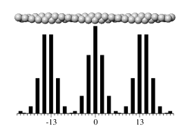
Figure 2: Target zones on an actin filament. The diagram shows the binding rate to the particular site if there is no longitudinal strain, i.e., if the head is horizontally aligned with the binding site. The binding rate has its maxima for actin subunits oriented downwards (towards the myosin-coated surface). The dimensionless angular stiffness is $\alpha=4$.

The force and the torque that a myosin head numbered $j$, bound to site $i$, exerts on the filament are

$$F^{j}=K(x^{j}_{M}+\delta-X-ia)\qquad M^{j}=-K_{\vartheta}(\Theta+i\vartheta_{0}+2\pi n)\;.$$ (4)

Here we introduced the displacement $\delta$ that has the value $0$ in the pre-powerstroke and $d=8\,\rm nm$ in the post-powerstroke and rigor state.

The simplified model for the duty cycle of the myosin head is defined as follows. A head binds to an actin site with the rate $k_{i}$ given by Eq. (2). The power stroke (a transition from $\delta=0$ do $\delta=d$) takes place with the rate $k_{PS}$. It is followed by the release of ADP with the rate $k_{-ADP}$. Detachment follows after binding a new ATP molecule, therefore its rate depends on the ATP concentration, $k_{D}=k_{D}^{0}\rm[ATP]$. We neglect the strain dependence of those rates, as well as the existence of the reverse transitions. It should be noted that in this formulation the model is not thermodynamically consistent. However, as we are only interested in dynamics at low loads, this does not significantly affect the results.

We assume that the filament position is quickly equilibrated after each step, therefore it always fulfills

$$F=\sum F^{j}=0\qquad M=\sum M^{j}=0\;.$$ (5)

Simulation results

Given the known structure of the actin helix and the power stroke size of myosin, our model essentially has two important parameters: the angular stiffness of myosin heads, $K_{\vartheta}$, and the ratio between the detachment- and the attachment rate, $k_{D}/k_{A}$. The latter is a function of the ATP concentration and is closely related to the duty ratio of motors. For other parameters we use the values given in Table 1. The power stroke, connected with the phosphate (Pi) release, is assigned a very fast rate, $k_{\rm PS}=10000\,{\rm s}^{-1}$, and can be considered as taking place immediately after binding. The maximum attachment rate $k_{A}$, i.e., the attachment rate to sites that do not require any elastic distortion, can be estimated as $50\,\rm s^{-1}$. This reflects the estimated average attachment rate of $30\,\rm s^{-1}$, or a maximum ATP turnover rate of $25\,\rm s^{-1}$ in muscle Howard_book . The ADP release takes place with the rate $k_{-ADP}=1000\,\rm s^{-1}$, characteristic for the fast myosin isoform Capitanio.Bottinelli2006 . For the detachment rate, which is determined by the ATP binding rate, we use $k_{D}^{0}=5\,\rm\mu M^{-1}s^{-1}$ Capitanio.Bottinelli2006 .

$k_{A}$	$50\,{\rm s}^{-1}$	Attachment rate
$k_{PS}$	$10000\,{\rm s}^{-1}$	Power stroke rate
$k_{-ADP}$	$1000\,{\rm s}^{-1}$	ADP release rate
$k_{D}$	$(5\,\rm\mu M^{-1}s^{-1})\rm[ATP]$	Detachment rate
$d$	$8\,\rm nm$	Power stroke size
$K$	$0.5\,\rm pN/nm$	Myosin stiffness (longitudinal)
$K_{\vartheta}=\alpha k_{B}T$		Myosin stiffness (angular)
$\alpha$	4, 6, 8	Dimensionless angular stiffness
$a$	$2.75\,\rm nm$	Distance between actin subunits
$\vartheta_{0}$	$-167.14^{\circ}$	Angle between actin subunits
$l$	$5.5\,\rm\mu m$	Actin filament length
$\rho$	$20\,\rm\mu m^{-1}$	1-d myosin density on surface
$k_{B}T$	$4.14\times 10^{-21}\rm J$	Thermal energy

Table 1: Simulation parameters

The stochastic simulation essentially followed the following algorithm:

1. Distribute the positions of myosin motors $x_{M}^{j}$ randomly along the distance covered by the actin filament, with an average linear density $\rho$. Set $X=0$ and $\Theta=0$.

2. Determine the total rate of all possible transitions as

   $$k_{\rm total}=\sum_{j\in\text{Motors}}\\ \left\{\begin{array}[]{ll}\sum_{i\in\text{Binding sites}}k_{A}^{i}(j)&\text{if motor $j$ detached}\\ k_{PS}&\text{if motor $j$ in pre-PS state}\\ k_{-ADP}&\text{if motor $j$ in post-PS state}\\ k_{D}&\text{if motor $j$ in rigor state}\end{array}\right.$$

   $k_{A}^{i}(j)$ is determined using Eq. (2) with the current values of $X$ and $\Theta$.

3. Determine the time until the next step as $\Delta t=k_{\rm total}^{-1}\ln(1/r)$, where $r$ is a random number between $0$ and $1$.

4. Choose randomly one of the possible steps (attachment, detachment, power stroke, ADP release), so that the probability of choosing a certain step is given by its rate, divided by $k_{\rm total}$.

5. Change the state of the chosen motor and update the filament position $X$ and angle $\Theta$ according to Eq. (5).

6. Continue with step 2 until $X\geq X_{\rm max}$ ($X_{\rm max}=1000\,\rm\mu m$).

7. Determine the average speed as $v=X/t$ and pitch as $\lambda=2\pi X/\Theta$.

(A)

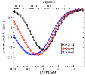
(B)

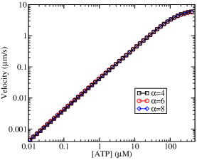
(C)

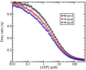
Figure 3: (A) Inverse twirling pitch (number of rotations per micron traveled) as a function of the ATP concentration. The lines represent 3 different values of the angular stiffness ($\alpha=4$, $\alpha=6$ and $\alpha=8$). Negative signs denote left-handed rotation. The upper scale shows the velocity (for $\alpha=4$). (B) Gliding velocity as a function of the detachment rate. (C) Duty ratio $\eta$, giving the average fraction of myosin heads in the bound state.

The results of this numerical simulation are shown in Fig. 3, which shows the inverse pitch of twirling as a function of the ATP concentration for three different values of the angular stiffness $K_{\vartheta}$. For reference, velocity (Fig. 3B) and duty ratio (Fig. 3C) are included as well. The behavior of the pitch is non-monotonous: it has a minimum of about $400-500\,\rm nm$ at intermediate speeds, but increases both at high, as well as very low speeds.

These results show that the helicity of the actin filament is sufficient to explain the twirling motion in a gliding assay. Somewhat counter-intuitively, this rotation is left-handed, and therefore opposite from the handedness of the actin filament. The effect becomes weaker for high speeds (where the distance traveled between two attachment events becomes longer), as well as for very low speeds, where motors have enough time to bind even to unfavorable sites outside the target zones.

Figure 4: Simplified model used for the analytical solution. The filament travels with a stationary velocity $v$ and rotates with an angular velocity $\omega$. $x$ denotes the position of a myosin anchoring point relative to the center of the target zone.

Analytical approximation

In the following we will describe an approximative analytical solution with the aim of understanding and quantitatively reproducing the twirling dynamics. The essential simplification we will make is to neglect the discrete nature of binding sites on the actin filament and replace them with a continuous helical “groove”. The simplified model is shown in Fig. 4. We denote each head with its root position $x$ relative to the center of the target zone:

$$x=x_{M}-\left(X-\frac{L}{\pi}\Theta+nL\right)$$ (6)

with $n$ such that $-\frac{L}{2}<x<\frac{L}{2}$. A bound head is additionally characterized by the strain $\xi$, which is the position of its root relative to its binding site. For for a head bound to site $i$, this is $\xi_{i}=x_{M}-X-ia$.

In the original model the total binding rate for a motor positioned at $x$ is

$$\bar{k}_{A}(x)=\sum_{i}k_{A}^{i}(x)=\sum_{i}k_{A}\exp\left[-\frac{K\xi_{i}^{2}+K_{\vartheta}\vartheta_{i}^{2}}{2k_{B}T}\right]\;.$$ (7)

In the sum, we only consider sites that are turned towards the motor-covered surface, therefore we can write the angle as

$$\vartheta_{i}=(x-\xi_{i})\frac{\pi}{L}$$ (8)

and by completing the square in the numerator we obtain

$$k_{A}^{i}(x)=k_{A}(x,\xi_{i})\\ =k_{A}\exp\left[-\frac{(K+K_{\vartheta}^{\prime})(\xi_{i}-\frac{K_{\vartheta}^{\prime}}{K+K_{\vartheta}^{\prime}}x)^{2}+\frac{KK_{\vartheta}^{\prime}}{K+K_{\vartheta}^{\prime}}x^{2}}{2k_{B}T}\right]\;.$$ (9)

In this equation we introduced the reduced angular stiffness $K_{\vartheta}^{\prime}=({\pi^{2}}/{L^{2}})K_{\vartheta}$. When we neglect the discreteness of binding sites and extend the summation beyond one period, we can replace the sum by an integral

$$\bar{k}_{A}(x) \approx\frac{1}{2a}\int_{-\infty}^{\infty}k_{A}(x,\xi)d\xi$$

$$=\frac{k_{A}}{2a}\sqrt{\frac{2\pi k_{B}T}{K+K_{\vartheta}^{\prime}}}\exp\left[-\frac{KK_{\vartheta}^{\prime}/(K+K_{\vartheta}^{\prime})x^{2}}{2k_{B}T}\right]\;.$$ (10)

For a fixed $x$, the the expected value of the strain at the time of attachment can be calculated using (9):

$$\left<\xi_{A}(x)\right>=\frac{\sum_{i}k_{A}^{i}(x)\xi_{i}}{\sum_{i}k_{A}^{i}(x)}\approx\frac{\int_{-\infty}^{\infty}k_{A}(x,\xi)\xi d\xi}{\int_{-\infty}^{\infty}k_{A}(x,\xi)d\xi}=\frac{K_{\vartheta}^{\prime}}{K+K_{\vartheta}^{\prime}}x$$ (11)

The expected value of the azimuthal angle at time of attachment follows from Eq. (8)

$$\left<\vartheta_{A}(x)\right>=\frac{K}{K+K_{\vartheta}^{\prime}}\left(\frac{\pi}{L}\right)x\;.$$ (12)

$L$	period (half-pitch) of the actin superhelix
$x$	motor root position relative to the center of the nearest target zone
$\xi$	motor root position relative to its binding site on actin
$k_{A}^{i}$	attachment rate to site $i$
$\bar{k}_{A}(x)$	total attachment rate for a motor positioned at $x$
$\left<\xi_{A}(x)\right>$	average strain of newly attached motors positioned at $x$
$\left<\xi_{A}\right>$	average strain of all newly attached motors
$\left<x_{A}\right>$	average position of newly attached motors, relative to the target zone
$\left<\vartheta_{A}\right>$	average angular strain at attachment
$v$	filament velocity
$c$	apparent velocity of the actin helix
$\omega$	angular velocity of actin rotation

Table 2: Variables used in the analytical calculation

In the stationary state, the filament moves with velocity $\dot{X}=v$ and rotates with angular velocity $\dot{\Theta}=\omega$. From Eq. (6) it follows that $\dot{x}=-(v-\frac{L}{\pi}\omega)=-c$. This is the apparent velocity with which the helix moves along the surface.

We can now set up a Master equation for the probability that a motor positioned at $x$ is in the attached state

$$\partial_{t}A(x,t)-c\partial_{x}A(x,t)=\bar{k}_{A}(x)(1-A(x,t))-k_{D}A(x,t)$$ (13)

and set $\partial_{t}A=0$ to obtain the stationary solution. $A$ also has to fulfill the periodic boundary condition

$$A(-L/2)=A(L/2)\;.$$ (14)

The expectation value of the attachment position can be calculated as

$$\left<x_{A}\right>=\frac{\int_{-L/2}^{L/2}x{\bar{k}}_{A}(x)(1-A(x))dx}{\int_{-L/2}^{L/2}{\bar{k}}_{A}(x)(1-A(x))dx}$$ (15)

and the average strain at the time of attachment follows from (11):

$$\left<\xi_{A}\right>=\frac{K_{\vartheta}^{\prime}}{K+K_{\vartheta}^{\prime}}\left<x_{A}\right>\;.$$ (16)

Because the strain on a motor changes with time as $\dot{\xi}=-v$, the average strain of all bound motors is $\left<\xi_{A}\right>-v/k_{D}$. The force per motor is then $F=K\left<\xi+d\right>=K(\left<\xi_{A}\right>-v/k_{D}+d$. As the total force produced by all motors has to be zero, we obtain an expression for the velocity

$$v=k_{D}(d+\left<\xi_{A}\right>)\;.$$ (17)

The same type of calculation as for the velocity can be made for the angular velocity. Motors attach with an average angle $\left<\vartheta_{A}\right>$. As the filament rotates, their angle changes as $\dot{\vartheta}=\omega$. The average angle of all motors is $\left<\vartheta_{A}\right>+\omega/k_{D}$ and needs to be zero because of torque balance, therefore

$$\omega=-k_{D}\left<\vartheta_{A}\right>=-k_{D}\frac{K}{K+K_{\vartheta}^{\prime}}\left(\frac{\pi}{L}\right)\left<x_{A}\right>\;.$$ (18)

These equations, together with the Master equation (13), the periodic boundary condition (14), the expression for $\left<\xi_{A}\right>$ (16) and for $\bar{k}_{A}$ (7) allow us to numerically determine the velocity $v$ and the distribution of attached heads $A(x)$ in a self-consistent manner. An example of the solution $A(x)$, along with the attachment rate $\bar{k}_{A}(x)$ and attachment flux $\bar{k}_{A}(x)(1-A(x))$ is shown in Fig. 5A. Well visible is the asymmetry in the attachment flux. The expectation value of $x$ at the time of attachment ($\left<x_{A}\right>$) as a function of the ratio $k_{D}/k_{A}$ is shown in Fig. 5B. It reaches its maximum when $k_{D}/k_{A}$ is such that each motor travels an average path of $\approx L/3$ between two attachment events.

(A)
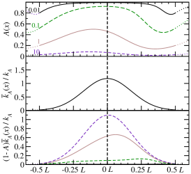
(B)

Figure 5: (A) Top panel: probability $A(x)$ that a motor with a position $x$ relative to the center of a target zone is in the bound state. The parameters are $k_{D}/k_{A}=0.01,0.1,1,10$ (each a different line type) and $\alpha=4$. Middle panel: dimensionless attachment rate ${\bar{k}}_{A}(x)/k_{A}$. Bottom panel: attachment flux, obtained as the product of the probability that a motor is in the detached state and the attachment rate. Note that the asymmetry is most pronounced for $k_{D}/k_{A}=0.1$. (B) The expectation value of $x$ at the time of binding, $\left<x_{A}\right>$, as a function of $k_{D}/k_{A}$.

This finally gives us the expression for the twirling pitch

$$\lambda=\frac{2\pi v}{\omega}=-\frac{2Ld\left(1+\frac{K_{\vartheta}^{\prime}}{K}\right)}{\left<x_{A}\right>}-2L\frac{K_{\vartheta}^{\prime}}{K}\;.$$ (19)

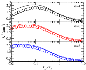
Figure 6: Inverse pitch $-\lambda^{-1}$, obtained from Eq. (19) (continuous line), and from simulation described in the previous section, however assuming $k_{-ADP}=\infty$. (circles). The top panel shows data for the angular stiffness $\alpha=4$, the middle $\alpha=6$ and the bottom $\alpha=8$. The minor deviation is mainly due to the extrapolations we made in regions between target zones. The agreement is better for large $\alpha$ values, where target zones become more localized.

The results are shown in Fig. 6 and compared with simulation data from Fig. 3. The simulation results are well reproduced, although there is a certain discrepancy which is more pronounced for low values of the angular stiffness $\alpha$. The main reason for this discrepancy is the extrapolation beyond the boundaries of one period, which was used in the derivation of Eq. (Analytical approximation). Other (minor) sources of deviation are the neglected discrete nature of binding sites and of the fact that each binding site can only be occupied by one head at a time.

Discussion

In this study we have demonstrated that the helical actin structure, along with the fact that myosin heads preferentially bind to those sites oriented towards them, is sufficient to explain left-handed rotation in a gliding assay. The maximum twirling motion is achieved at relatively low speeds (below $100\,\rm nm/s$). Twirling is reduced with higher speeds, achieved at higher ATP concentrations. Interestingly, it is also reduced under extremely low ATP concentrations, when the velocity drops under $10\,\rm nm/s$. However, in this regime the results depend strongly on the choice of the angular stiffness $\alpha$, which is less well known. The minimum pitch resulting from this effect lies in the order of $400$–$500\,\rm nm$, which is in good agreement with recent experimental results Beausang.Goldman2008 . The model also makes a testable prediction that the pitch should increase with a higher ATP concentration. Because pitch only depends on the ratio between the attachment and detachment rate, addition of ADP should have the same effect on the pitch as a reduced ATP concentration that yields the same filament speed. If this turns out not to be the case, it will be a strong indication of a lateral conformational change in the myosin head connected with the release of ADP.

Although the qualitative aspects of our theory are generic and practically independent of any assumptions other than the helical actin structure, there are alternative effects that could well contribute to the twirling motion. One such possibility is that the power-stroke of the myosin head contains a lateral (azimuthal, off-axis) component. A similar effect could also result from an asymmetric attachment rate, which could cause the attached motors to exert a certain torque on the filament immediately after binding. Such a torque does not contradict the laws of thermodynamics because the first bound state is not in equilibrium with the detached state. A related idea is described by Beausang et al. Beausang.Goldman2008 as the “rigor drag model” in which heads in the rigor state exert a torque in the opposite direction from that immediately after binding. This results in a pitch that depends on the fraction of time spent in the rigor state. The important difference between the two concepts is that in our model the torque generated by newly attached myosin heads depends on the ATP concentration, whereas in the rigor drag model this torque is constant and the variable pitch is caused by different dwell times in different states.

In any case both the effect described here and the explicit lateral component of the power stroke will be superimposed. So it is theoretically possible, even though the proposition is purely speculative at the moment, that the power stroke might have the opposite helicity, i.e., it would lead to a right-handed filament rotation. In such a case, there could be a cross-over form right handed motion under high ATP concentrations, to left-handed under low. This is could be one possibility to reconcile the recent results Beausang.Goldman2008 with those by Nishizaka et al. nishizaka93 .

Recent experiments also revealed rotation of microtubules moved by monomeric kinesin-1 Yajima.Cross2005 and Eg5 Yajima.Nishizaka2008 . The theory we presented in this paper is not applicable to microtubules, because they have no distinct target zones. Any rotation resulting from an effect of the kind we describe here would be negligible. Therefore, as suggested in Yajima.Cross2005 , the rotation caused by kinesins has to result from a lateral (off-axis) component of a power stroke, or from an asymmetry in the binding rate.

Appendix

In the following we will discuss how the simplified model, which assumes that motors are distributed one-dimensionally underneath the actin filament, and which we use throughout the main text, relates to the full two-dimensional model. In the 2-D model, which describes the actual situation in a gliding assay, myosin heads are distributed all over the glass surface and their positions are described with two coordinates, $(x_{M}^{j},y_{M}^{j})$. The position of the actin filament is described with the coordinates $(X,Y)$ and the angle $\Theta$. We assume that the filament keeps its direction parallel to the $X$-axis. The elastic distortion of the head $j$ binding to the site $i$ can then be written as

$$U_{i}=\frac{1}{2}K(X+ia-x_{M}^{j})^{2}+U_{A}(\Theta+i\vartheta_{0},Y-y_{M}^{j})$$ (20)

where $U_{A}$ is an unknown function of the azimuth angle of binding site $i$ and of the lateral position of the filament relative to the motor.

The total binding rate to site $i$ of all motors located at longitudinal position $x_{M}$ is then

$$k_{A}(x_{M})\\ =\int_{-\infty}^{\infty}k_{A}\exp\left[-\frac{U_{i}(X+ia-x_{M},\Theta+i\vartheta_{0},Y-y_{M})}{k_{B}T}\right]\\ \times\rho D(x_{M},y_{M})dy_{M}$$ (21)

where $\rho$ is the 2-D surface density of myosin motors and $D(x_{M},y_{M})$ the probability that a motor at that position is in the detached state. If we assume that $D(x_{M},y_{M})=D(x_{M},2Y-y_{M})$, i.e., that the distribution of unbound heads is symmetric with respect to the filament, the resulting function $k_{A}(x_{M})$ has to be symmetric in $\Theta+i\vartheta_{0}$. We can therefore approximate it with the expression used in Eqs. (1,2).

The average torque generated by a head that binds to site $i$ can be calculated as

$$\left<M\right> =-\frac{\int_{-\infty}^{\infty}\exp\left(-U_{i}/k_{B}T\right)D(x_{M},y_{M})\left(\partial U_{i}/\partial\Theta\right)dy_{M}}{\int_{-\infty}^{\infty}\exp\left(-U_{i}/k_{B}T\right)D(x_{M},y_{M})dy_{M}}$$

$$=\frac{k_{B}T}{k_{A}(x_{M})}\frac{dk_{A}(x_{M})}{d\Theta}\;.$$ (22)

This second expression is equivalent to that in the 1-D model.

The average force generated by a head that binds to site $i$ is determined the same way:

$$\left<F_{L}\right>=-\frac{\int_{-\infty}^{\infty}\exp\left(-U_{i}/k_{B}T\right)D(x_{M},y_{M})\left(\partial U_{i}/\partial Y\right)dy_{M}}{\int_{-\infty}^{\infty}\exp\left(-U_{i}/k_{B}T\right)D(x_{M},y_{M})dy_{M}}\;.$$ (23)

If $D(x_{M},y_{M})$ is independent of $y_{M}$, or, more generally, if it has a dependence that can be written as a function of $U_{i}$, the integral in the numerator is 0 and there is no lateral force. However, with different distributions $D(x_{M},y_{M})$, a small lateral force is possible, so that the filament could show some sideways motion in the 2-D model. While the torque results from a $D(x_{M},y_{M})$ which is asymmetric in $x_{M}$, a lateral force needs asymmetry in both coordinates and is therefore a higher-order effect.

References

- (1) Toyoshima, Y. Y., S. J. Kron, E. M. McNally, K. R. Niebling, C. Toyoshima, and J. A. Spudich. 1987. Myosin subfragment-1 is sufficient to move actin filaments in vitro. Nature 328:536–539.
- (2) Howard, J., A. J. Hudsepth, and R. D. Vale. 1989. Movement of microtubules by single kinesin molecules. Nature 342:154–158.
- (3) Duke, T., E. Holy, and S. Leibler. 1995. “Gliding Assays” for Motor Proteins: A Theoretical Analysis. Phys. Rev. Lett. 74:330–333.
- (4) Bourdieu, L., T. Duke, M. B. Elowitz, D. A. Winkelmann, S. Leibler, and A. Libchaber. 1995. Spiral Defects in Motility Assays: A Measure of Motor Protein Force. Phys. Rev. Lett. 75:176–179.
- (5) Gibbons, F., J. F. Chauwin, M. Desposito, and J. V. Jose. 2001. A dynamical model of kinesin-microtubule motility assays. Biophys. J. 80:2515–2526.
- (6) Tanaka, Y., A. Ishijima, and S. Ishiwata. 1992. Super helix formation of actin filaments in an in vitro motile system. Biochim. Biophys. Acta 1159:94 – 98.
- (7) Nishizaka, T., T. Yagi, Y. Tanaka, and S. Ishiwata. 1993. Right-handed rotation of an actin filament in an in vitro motile system. Nature 361:269–271.
- (8) Sase, I., H. Miyata, S. Ishiwata, and K. Kinosita, Jr.. 1997. Axial rotation of sliding actin filaments revealed by single-fluorophore imaging. Proc. Natl. Acad. Sci. USA 94:5646–5650.
- (9) Ali, M. Y., S. Uemura, K. Adachi, H. Itoh, K. Kinosita, Jr., and S. Ishiwata. 2002. Myosin V is a left-handed spiral motor on the right-handed actin helix. Nat. Struct. Biol. 9:464–467.
- (10) Vilfan, A. 2005. Elastic lever-arm model for myosin V. Biophys. J. 88:3792–3805.
- (11) Vilfan, A. 2005. Influence of fluctuations in actin structure on myosin V step size. J. Chem. Inf. Model. 45:1672–1675.
- (12) Ali, M. Y., K. Homma, A. H. Iwane, K. Adachi, H. Itoh, K. Kinosita, Jr., T. Yanagida, and M. Ikebe. 2004. Unconstrained steps of myosin VI appear longest among known molecular motors. Biophys. J. 86:3804–3810.
- (13) Sun, Y., H. W. Schroeder III, J. F. Beausang, K. Homma, M. Ikebe, and Y. E. Goldman. 2007. Myosin VI walks “wiggly” on actin with large and variable tilting. Mol. Cell 28:954–964.
- (14) Arsenault, M. E., Y. Sun, H. H. Bau, and Y. E. Goldman. 2009. Using electrical and optical tweezers to facilitate studies of molecular motors. Phys. Chem. Chem. Phys. In press, DOI 10.1039/b821861g.
- (15) Beausang, J. F., H. W. Schroeder III, P. C. Nelson, and Y. E. Goldman. 2008. Twirling of actin by myosins II and V observed via polarized TIRF in a modified gliding assay. Biophys. J. 95:5820–5831.
- (16) Purcell, T. J., H. L. Sweeney, and J. A. Spudich. 2005. A force-dependent state controls the coordination of processive myosin V. Proc. Natl. Acad. Sci. USA 102:13873–13878.
- (17) Steffen, W., D. Smith, R. Simmons, and J. Sleep. 2001. Mapping the actin filament with myosin. Proc. Natl. Acad. Sci. USA 98:14949–14954.
- (18) Capitanio, M., M. Canepari, P. Cacciafesta, V. Lombardi, R. Cicchi, M. Maffei, F. S. Pavone, and R. Bottinelli. 2006. Two independent mechanical events in the interaction cycle of skeletal muscle myosin with actin. Proc. Natl. Acad. Sci. USA 103:87–92.
- (19) Vilfan, A., and T. Duke. 2003. Instabilities in the transient response of muscle. Biophys. J. 85:818–826.
- (20) Veigel, C., M. L. Bartoo, C. S. White, J. S. Sparrow, and J. E. Molloy. 1998. The stiffness of rabit skeletal acotmyosin cross-bridges determined with an optical tweezers transducer. Biophys. J. 75:1424.
- (21) Howard, J. 2001. Mechanics of Motor Proteins and the Cytoskeleton. Sinauer, Sunderland, MA.
- (22) Yajima, J., and R. A. Cross. 2005. A torque component in the kinesin-1 power stroke. Nat. Chem. Biol. 1:338–341.
- (23) Yajima, J., K. Mizutani, and T. Nishizaka. 2008. A torque component present in mitotic kinesin Eg5 revealed by three-dimensional tracking. Nat. Struct. Mol. Biol. 15:1119–1121.