The Next-to-Minimal Supersymmetric extension of the Standard Model reviewed

Abstract

The next-to-minimal supersymmetric extension of the Standard Model (NMSSM) is one of the most favored supersymmetric models. After an introduction to the model, the Higgs sector and the neutralino sector are discussed in detail. Theoretical, experimental, and cosmological constraints are studied. Eventually, the Higgs potential is investigated in the approach of bilinear functions. Emphasis is placed on aspects which are different from the minimal supersymmetric extension.

1 Introduction

Supersymmetry (Ramond:1971gb, ; Neveu:1971rx, ; Gervais:1971ji, ; Golfand:1971iw, ; Wess:1974tw, ; Volkov:1973ix, ; Fayet:1976et, ; Fayet:1977yc, ; Farrar:1978xj, ; Fayet:1979sa, ; Witten:1981nf, ; Dimopoulos:1981zb, ; Sakai:1981gr, ; Ohta:1982wn, ; Nilles:1983ge, ; Haber:1984rc, ; Gunion:1984yn, ; Gunion:1986nh, ; Lahanas:1986uc, ) is one of the most appealing concepts of physics beyond the Standard Model (SM). Some of the main motivations for studying supersymmetry are:

• Supersymmetry is an extension of the Poincare algebra which relates fermions to bosons.

• As a local symmetry, supersymmetry is naturally connected to gravity.

• Supersymmetry stabilizes the hierarchy (Witten:1981kv, ; Polchinski:1982an, ; Dimopoulos:1981zb, ; Sakai:1981gr, ) between the electroweak and the GUT or Planck scale. Thus, the quadratical divergences occurring in the Higgs-boson mass loop corrections are systematically canceled and fine tuning between the bare Higgs-boson mass and the loop contributions is avoided.

• Supersymmetry, realized below the TeV scale, unifies the $SU(3)_{C}\times SU(2)_{L}\times U(1)_{Y}$ couplings at the GUT scale.

• Supersymmetry provides a cold dark matter candidate, supposed matter-parity is conserved.

A minimal supersymmetric extension of the Standard Model (MSSM) was proposed already some time ago. For a review of the MSSM see for instance (Martin:1997ns, ) and references therein. In the MSSM the minimal particle content is added to the SM in order to arrive at a supersymmetric model. The MSSM extents the SM by an additional Higgs doublet, necessary to give masses to up- and down-type fermions and in order to keep the theory anomaly free. Every field is promoted to a superfield, pairing fermionic and bosonic degrees of freedom. However, none of the additional predicted particles has been observed up to now. Thus the question arises, why should we study further extensions of the minimal supersymmetric model? The reason is, that the MSSM does certainly not parameterize any supersymmetric extension of the SM. This is in particular due to the fixed particle content we encounter in the MSSM. For instance, although the Higgs sector in the MSSM consists of two doublets in contrast to one in the SM, the Higgs sector turns out to be highly restricted. Thus, at tree-level, the lightest CP-even Higgs-boson is predicted to be lighter than the $Z$-boson. Large quantum corrections are necessary in order to comply with the experimental lower bounds from LEP on the CP-even Higgs-boson mass, which in turn require a very large scalar–top mass. That is, some new kind of fine-tuning is to be introduced in the MSSM.

Let us collect some reasons, making it worthwhile to study extensions of the minimal supersymmetric Standard Model:

• In the MSSM we encounter the so-called $\mu$-term in the superpotential, where $\mu$ is a dimensionful parameter. This parameter has to be adjusted by hand to a value at the electroweak scale, before spontaneous symmetry breaking occurs (Kim:1983dt, ). This is seen to be a problem of the model. It is desirable to look for further extension, which do not have this $\mu$-problem. In singlet extensions, for instance, an effective $\mu$-term may be generated dynamically.

• As mentioned before, the Higgs sector is highly restricted in the MSSM. The lower bounds on the Higgs-boson masses from LEP measurements require large quantum corrections accompanied by a large stop mass in this model. An extended Higgs sector may relax this restrictions and thus circumvent the lower experimental bounds.

• The MSSM Higgs-boson sector is CP-conserving at tree level. Extending the Higgs sector in an appropriate way, CP violating phases arise. Sufficient CP-violation would meet one of the necessary Sakharov criteria (Sakharov:1967dj, ) in order to generate the baryon–antibaryon asymmetry in our Universe.

• The baryon–antibaryon asymmetry may be generated by strong electroweak phase transitions of first order (Kuzmin:1985mm, ; Shaposhnikov:1987tw, ; Rubakov:1996vz, ; Shaposhnikov:1996th, ). The required cubic terms in the effective potential arise in the SM and the MSSM only via generically small radiative corrections. An explicit cubic term is possible in extensions of the MSSM.

Here we will review the next-to-minimal supersymmetric extension of the Standard Model (NMSSM) (Fayet:1974pd, ; Dine:1981rt, ; Nilles:1982dy, ; Derendinger:1983bz, ; Frere:1983ag, ; Veselov:1985gd, ; Ellis:1988er, ; Ellwanger:1993xa, ; King:1995vk, ; Ellwanger:1996gw, ; Franke:1995tc, ; Ananthanarayan:1996zv, ; Ellwanger:1999ji, ), which has the capability to solve the mentioned limitations of the MSSM. In the NMSSM an additional gauge singlet is introduced which generates the $\mu$-term dynamically, that is, an effective $\mu$-term arises spontaneously and the adjustment by hand drops out. This is surely the main motivation for the NMSSM and may justify the price to pay, that is, the introduction of an additional gauge-singlet superfield. The particle content in the bosonic part of the singlet results in two additional Higgs bosons whereas in the fermionic part we have one additional neutralino, called singlino. Altogether we have seven Higgs bosons and five neutralinos in the NMSSM, compared to five Higgs bosons and four neutralinos in the MSSM. The Higgs-boson sector of the NMSSM is no longer CP-conserving at tree level, merely CP-conservation only arises if the parameters of the Higgs-boson sector are chosen in an appropriate way. Nevertheless, in most studies in the literature the special case of a CP-conserving Higgs sector is considered, in order to simplify matters. In case of a CP-conserving Higgs sector we encounter altogether three CP-even Higgs-bosons, two CP-odd ones and in addition two charged Higgs bosons in the next-to-minimal model. As we will see, the Higgs-boson sector is in deed much less restricted and the lower mass bound prediction of a CP-even Higgs boson in the MSSM is generally shifted substantially. The Higgs-boson phenomenology can in general be very different from what to expect in the MSSM; in addition to supplement the total number of Higgs-bosons. For instance, in the NMSSM the possibility arises that a CP-even Higgs boson decays into two very light CP-odd ones which would have escaped detection at LEP and may even be difficult to detect at the LHC. Also the Higgs potential is enriched, leading to interesting consequences. Let us also address the last aforementioned advantage of the NMSSM over the MSSM. As we will see, the trilinear $A$-parameter soft supersymmetry breaking terms, corresponding to the superpotential, may account for the desired strong first order electroweak phase transition without large fine-tuning.

The additional neutralino, that is, the singlino, in general mixes with the other four neutralinos. Also in the neutralino sector there may be a substantial change of phenomenology compared to the minimal supersymmetric model; in addition to supplement the total number of neutralinos by a fifth neutralino. This is due to the fact that the singlino is introduced as a gauge singlet. Only through mixing with the other neutralinos this singlino has couplings to the non-Higgs particles. This opens the intriguing possibility to have a singlino-like neutralino which moreover may become the lightest supersymmetric (partner-)particle (LSP). Relying on matter-parity, every supersymmetric partner particle will in this case eventually decay into this singlino-like LSP. In particular the next-to-lightest supersymmetric (partner-)particle (NLSP) would, due to the small couplings, decay very slowly into the LSP. These large decay length’ could be revealed by signatures of displaced vertices in the detector. But of course, in case the singlino-like neutralino is not the LSP, it would be omitted or at least be suppressed in cascade decays. Generally, in discussing the NMSSM phenomenology we draw the attention to differences to the MSSM. For the MSSM phenomenology we refer to the extensive literature to this subject.

We start in Sect. 2 with the NMSSM superpotential. We review the main motivations for the modifications compared to the MSSM and also discuss the drawback which arises in context with the Peccei–Quinn symmetry, which is promoted to a discrete $\mathbbm{Z}_{3}$-symmetry by the introduction of the singlet cubic selfcoupling in the superpotential. We recall the arguments in order to circumvent the occurrence of dangerous domain walls which emerge in context of spontaneously broken discrete symmetries.

In Sect. 3 we present the mass matrices and the parameters to describe the complete Higgs-boson sector at tree-level. In this we treat the most general Higgs sector with the possibility of CP-violation. The special case of a CP-conserving Higgs sector may be easily inferred. We briefly mention the one-loop effective potential involving the field-dependent Higgs-boson masses. Then we discuss the Higgs-boson phenomenology, where we stress the prospects at the LHC. In particular we review the discussion of a “no-lose” theorem, that is, the interesting question, whether it can be guaranteed that at least one Higgs boson of the NMSSM will be detected at the LHC - supposed the NMSSM is realized in Nature.

In Sect. 4 follows a recap of the neutralino sector, where we present the mixing matrix as well as neutralino phenomenology, which is of special interest in case there is a singlino-like LSP.

In Sect. 5 we consider parameter constraints in the NMSSM, beginning with theoretical constraints. For instance a theoretical constraint comes from the requirement to have a potential with a global minimum not breaking electric or color charge. A further constraint restricts coupling parameters by forcing them to be perturbative up to the GUT scale. Of course the latter constraint relies on the fact that the model is valid in the large range up to the GUT scale. We will also discuss briefly an approach to quantify fine-tuning in general extensions of the SM. On the experimental side we start with considering constraints coming from colliders. Precision measurements of the $Z$-boson width are discussed, followed by exclusion limits from searches for neutralino and chargino pair production, as well as Higgs-boson production. The possible contribution of the NMSSM to the anomalous magnetic moment of the muon is discussed. The constraints from the $b\rightarrow s\gamma$ decay are presented, which is a loop induced process and thus highly sensitive to possible new particles emerging in the loops. Turning to cosmology we start with the very strong constraint origination from the new WMAP result on the relic abundances of the LSP, supposed this is the candidate for the observed cold dark matter. The direct dark matter detection experiments are recalled briefly. Eventually we discuss the prospects of the NMSSM in terms of strong first order electroweak phase transitions in order to explain the baryon–antibaryon asymmetry. Finally, we consider some of the newer parameter scans, which provide some interesting insight for rather large ranges of parameter space.

In section 6 we inspect the Higgs potential with respect to stationary solutions. A method is introduced employing a Groebner basis approach in the framework of gauge invariant functions. This method allows to certainly determine the global minimum and reveals a quite surprising stationarity structure. However, the Groebner basis approach is restricted to the tree-level potential.

We close with a rather extended appendix. We mention some of the frequently used computer tools, mainly used in parameter scans, followed by a derivation of the essential new Feynman rules in the NMSSM compared to the MSSM. Then we present the formalism of gauge-invariant functions as well as the Buchberger algorithm which allows to compute a Groebner basis, employed in the determination of the global minimum.

In advance we apologize for any missing references in the bibliography. But in view of the vast amount of publications with view on the NMSSM, in particular in the recent years, this seems to be hardly avoidable.

2 The NMSSM superpotential

In the NMSSM the superpotential is

$$W=\hat{{u}}y_{u}(\hat{Q}^{\mathrm{T}}\epsilon\hat{H}_{u})-\hat{{d}}y_{d}(\hat{Q}^{\mathrm{T}}\epsilon\hat{H}_{d})-\hat{{e}}y_{e}(\hat{L}^{\mathrm{T}}\epsilon\hat{H}_{d})+\lambda\hat{S}(\hat{H}_{u}^{\mathrm{T}}\epsilon\hat{H}_{d})+\frac{1}{3}\kappa\hat{S}^{3}$$ (1)

with dimensionless couplings $y_{u}$, $y_{d}$, $y_{e}$, $\lambda$ and $\kappa$. Note that the superpotential has cubic mass dimension. The supermultiplets are denoted with a hat and are given in Tab. 1 together with its bosonic and fermionic particle content and its multiplicity respectively hypercharge with respect to $SU(3)_{C}\times SU(2)_{L}\times U(1)_{Y}$. Compared to the MSSM particle content there is only one new supermultiplet ingredient, namely the gauge singlet $\hat{S}$, that is, one complex spin-0 singlet $S$ and one spin-1/2 singlino $\tilde{S}$. The weak isospin indices are not written explicitly and $\epsilon$ is defined below in (21). Note that the convention for the signs of the $\lambda$ and $\kappa$ terms in the superpotential differ in the literature.

chiral supermultiplets		spin-$0$	spin-$1/2$	$SU_{C}(3)$	$SU_{L}(2)$	$U_{Y}(1)$
quark–squark Q	$\hat{Q}$	$\tilde{Q}=(\tilde{u}_{L},\;\tilde{d}_{L})^{\mathrm{T}}$	$Q=({u}_{L},\;{d}_{L})^{\mathrm{T}}$	$\mathbf{3}$	$\mathbf{2}$	$\phantom{+}1/6$
	$\hat{u}$	$\tilde{u}_{R}^{*}$	$u_{R}^{\dagger}$	$\mathbf{3}$	$\mathbf{1}$	$-2/3$
	$\hat{d}$	$\tilde{d}_{R}^{*}$	$d_{R}^{\dagger}$	$\mathbf{3}$	$\mathbf{1}$	$\phantom{+}1/3$
lepton–slepton	$\hat{L}$	$\tilde{L}=(\tilde{\nu}_{e},\;\tilde{e}_{L})^{\mathrm{T}}$	$L=({\nu_{e}},\;{e}_{L})^{\mathrm{T}}$	$\mathbf{1}$	$\mathbf{2}$	$-1/2$
	$\hat{e}$	$\tilde{e}_{R}^{*}$	$e_{R}^{\dagger}$	$\mathbf{1}$	$\mathbf{1}$	$\phantom{+}1$
Higgs–Higgsino	$\hat{H}_{u}$	${H}_{u}=(H^{+}_{u},\;H^{0}_{u})^{\mathrm{T}}$	$\tilde{H}_{u}=(\tilde{H}^{+}_{u},\;\tilde{H}^{0}_{u})^{\mathrm{T}}$	$\mathbf{1}$	$\mathbf{2}$	$\phantom{+}1/2$
	$\hat{H}_{d}$	${H}_{d}=(H^{0}_{d},\;H^{-}_{d})^{\mathrm{T}}$	$\tilde{H}_{d}=(\tilde{H}^{0}_{d},\;\tilde{H}^{-}_{d})^{\mathrm{T}}$	$\mathbf{1}$	$\mathbf{2}$	$-1/2$
	$\hat{S}$	$S$	$\tilde{S}$	$\mathbf{1}$	$\mathbf{1}$	$\phantom{+}0$
gauge supermultiplets		spin-$1/2$	spin-$1$	$SU_{C}(3)$	$SU_{L}(2)$	$U_{Y}(1)$
gluon–gluino		$\tilde{g}$	$g$	$\mathbf{8}$	$\mathbf{1}$	$\phantom{+}0$
W-boson–wino		$\tilde{W}^{\pm},\tilde{W}^{0}$	${W}^{\pm},{W}^{0}$	$\mathbf{1}$	$\mathbf{3}$	$\phantom{+}0$
B-boson–bino		$\tilde{B}^{0}$	$B^{0}$	$\mathbf{1}$	$\mathbf{1}$	$\phantom{+}0$

Table 1: Particle content of the NMSSM in terms of decomposed supermultiplets together with the corresponding multiplicity respectively hypercharge with respect to $SU(3)_{C}\times SU(2)_{L}\times U(1)_{Y}$. Compared to the particle content of the minimal supersymmetric extension the new ingredient in the next-to-minimal extension is the Higgs supermultiplet $\hat{S}$. Only the first family is given; the other families are introduced analogously. The here used convention for the hypercharge is $Q=I_{W}^{3}+Y_{W}$ with $Q$ the electromagnetic charge in units of the positron charge, $I_{W}^{3}$ the weak isospin 3-component, and $Y_{W}$ the hypercharge.

2.1 Discussion of the superpotential

We start from the MSSM potential in terms of scalar fields,

$$W_{\text{MSSM}}=\tilde{u}_{R}^{*}y_{u}(\tilde{Q}^{\mathrm{T}}\epsilon H_{u})-\tilde{d}_{R}^{*}y_{d}(\tilde{Q}^{\mathrm{T}}\epsilon H_{d})-{\tilde{e}_{R}^{*}}y_{e}(\tilde{L}^{\mathrm{T}}\epsilon H_{d})+\mu(H_{u}^{\mathrm{T}}\epsilon H_{d})\,.$$ (2)

This is the minimal superpotential, where we have instead of the dimensionless terms $\lambda{S}\left(H_{u}^{\mathrm{T}}\epsilon H_{d}\right)+\frac{1}{3}\kappa S^{3}$ a so-called $\mu$-term, with $\mu$ a dimensionful parameter. In any case a term proportional to $H_{u}^{\mathrm{T}}\epsilon H_{d}$ is required to give masses to up- and down-type fermions. This follows immediately from the F-terms derived from the superpotential; as given in (145). Now, we know from experiment that the Higgs vacuum-expectation-value is $v\approx 246$ GeV, that is, of the order of the electroweak scale. With view on the F- and soft-breaking terms in the MSSM potential we get potential terms $\left(|\mu|^{2}+m_{H_{u}}^{2}\right)|H_{u}^{0}|^{2}+\left(|\mu|^{2}+m_{H_{d}}^{2}\right)|H_{d}^{0}|^{2}$. (This can be seen in the following discussion of the Higgs potential and can be read off from (22) and (25) if we replace $|\lambda|^{2}|S|^{2}$ by $|\mu|^{2}$). With the vacuum-expectation-values $\langle H_{d}^{0}\rangle=v_{d}/\sqrt{2}$, $\langle H_{u}^{0}\rangle=v_{u}/\sqrt{2}$ and $v^{2}=v_{u}^{2}+v_{d}^{2}$ we see that without fine-tuning between the mass- and $\mu$-parameters, the parameter $\mu$ can not be much larger than $v$. This is, that we have to adjust the $\mu$-parameter by hand to the electroweak scale which in the SM arises from spontaneous symmetry breaking. This is the so-called $\mu$-problem of the MSSM.

2.1.1 Peccei–Quinn symmetry

The main idea is to circumvent this dimensionful parameter $\mu$ by introducing a new scalar field $S$ which gets a vacuum expectation value to generate this parameter effectively, that is, the $\mu$-term is replaced by $\lambda{S}\left(H_{u}\epsilon H_{d}\right)$ and the required $\mu$-term at the electroweak scale arises from spontaneous symmetry breaking with $\mu=\lambda\langle S\rangle$. In this way we have achieved a quasi-universal mechanism of spontaneous symmetry breaking. This is considered to be the main motivation of the NMSSM. For some other solutions to circumvent the $\mu$-problem we refer the reader to App. E. Now, since the bilinear $\mu$-term in the superpotential is replaced by a trilinear term, we can see that the superpotential is invariant under a global phase transformation, the so-called Peccei–Quinn (PQ) symmetry $U(1)_{PQ}$  (Fayet:1974pd, ; Peccei:1977ur, ; Peccei:1977hh, ). If we assign PQ charges $q_{\text{PQ}}$ to the chiral supermultiplets, denoted by $\hat{\phi}_{i}$ with $i$ running over all chiral supermultiplets, in the following way (Fayet:1974pd, ; Panagiotakopoulos:1998yw, ),

$$\begin{array}[]{l|c|c|c|c|c|c|c|c}\text{supermultiplet }\hat{\phi}_{i}&\hat{Q}&\hat{u}&\hat{d}&\hat{L}&\hat{e}&\hat{H}_{u}&\hat{H_{d}}&\hat{S}\\ \hline\cr\text{PQ-charge }q_{\text{PQ}}&-1&0&0&-1&0&+1&+1&-2\end{array}\,,$$ (3)

we see immediately that the superpotential is invariant under the global $U(1)_{PQ}$ transformations

$$\hat{\phi}_{i}\rightarrow e^{iq_{\text{PQ}}\theta}\hat{\phi}_{i}\;,$$ (4)

with an arbitrary phase $\theta$. Note that since we assign PQ-charges to supermultiplets also the derived Lagrangian stays invariant under $U(1)_{PQ}$. In the minimal supersymmetric extension, MSSM, the PQ symmetry is explicitely broken by the $\mu$-term. In the NMSSM this PQ-symmetry is spontaneously broken once the Higgs bosons acquire vacuum-expectation-values. This spontaneous broken continuous symmetry gives, following the Goldstone theorem, inevitable a massless so-called Peccei–Quinn mode. Such axion has not been found and exclusion limits were derived (Hagiwara:2002fs, ). Experimentally there remains only a rather small corresponding $\lambda$-parameter occurring in the superpotential term $\lambda\hat{S}(\hat{H}_{u}^{\mathrm{T}}\epsilon\hat{H}_{d})$ in the range $10^{-7}<|\lambda|<10^{-10}$. In order to get an effective $\mu$ term of the electroweak order, the vacuum-expectation-value (VEV) of $S$ would have to be much larger compared to the electroweak scale - again a fine-tuning would be required.

In the NMSSM thus an additional term is imposed in the superpotential in oder to violate the Peccei-Quinn symmetry by means of a cubic selfcoupling term, $\frac{1}{3}\kappa\hat{S}^{3}$, with $\kappa$ the PQ-symmetry breaking parameter. In this way all parameters of the superpotential are still dimensionless. Alternatively, one could impose a linear or quadratic term in order to break the Peccei-Quinn symmetry but then again a dimensionful parameter would be necessary. Note that the superpotential has to have mass dimension three. Of course any term higher than trilinear in the fields in the superpotential is forbidden by the requirement of renormalizability. Finally we arrive at the proposed NMSSM superpotential, written in its scalar form

$$W=\tilde{u}_{R}^{*}y_{u}(\tilde{Q}^{\mathrm{T}}\epsilon H_{u})-\tilde{d}_{R}^{*}y_{d}(\tilde{Q}^{\mathrm{T}}\epsilon H_{d})-{\tilde{e}_{R}^{*}}y_{e}(\tilde{L}^{\mathrm{T}}\epsilon H_{d})+\lambda{S}(H_{u}^{\mathrm{T}}\epsilon H_{d})+\frac{1}{3}\kappa S^{3}\;.$$ (5)

2.1.2 Discrete $\mathbbm{Z}_{3}$ symmetry

There is some debate, whether the NMSSM superpotential (5) is viable. The main concern arises since the continuous Peccei-Quinn symmetry is broken explicitly by the $\frac{1}{3}\kappa S^{3}$ term, but there remains a discrete $\mathbbm{Z}_{3}$ symmetry of the superpotential (Zeldovich:1974uw, ):

$$\hat{\phi}_{i}\rightarrow e^{i\frac{2\pi}{3}}\hat{\phi_{i}}\,,$$ (6)

where the index $i$ runs over all superfields occurring in the superpotential. This discrete symmetry is spontaneously broken by the VEV of the complex scalar field $S$. Inevitably, this spontaneous breaking of a discrete symmetry leads to the domain-wall problem, a special kind of a topological defect. During electroweak phase transition of the early Universe, this spontaneously broken discrete symmetry would cause a dramatic change of the evolution of the Universe and would spoil the observed cosmic microwave background radiation.

A study of the generation of domain walls in the NMSSM potential with numerical methods can be found in (Abel:1995uc, ). Following (Zeldovich:1974uw, ; Vilenkin:1986hg, ) we want to sketch the mechanism of the formation of domain walls in a model with spontaneous breaking of a discrete symmetry in the simple Goldstone model of a complex scalar field $\phi$ with Lagrangian

$${\cal L}=\frac{1}{2}(\partial_{\mu}\phi^{\dagger})(\partial^{\mu}\phi)-\frac{\lambda}{4}\left(\phi^{2}-\eta^{2}\right)^{2},$$ (7)

where $\eta$ is a constant. The potential of this Lagrangian is the double well potential. The minima of the potential are at

$$\phi_{\pm}=\pm\eta,$$ (8)

that is, we have in this case a discrete $\mathbbm{Z}_{2}$ symmetry of the Lagrangian which is spontaneously broken by the vacuum. Now, the domain wall is nothing but the intermediate region between these degenerate minima $\phi_{\pm}$. Let us assume, without loss of generality, that this domain wall is situated in the $y$-$z$-direction. From the Goldstone-model Lagrangian we determine the Euler–Lagrange equation $\phi+\lambda\phi\left(\phi^{2}-\eta^{2}\right)=0$. The solution of this equation is

$$\phi=\eta\tanh(\frac{x}{\Delta}),$$ (9)

with thickness of the wall $\Delta\equiv(\lambda/2)^{-1/2}\eta^{-1}$. This solution describes the field in the intermediate domain-wall region between the two vacua. We see that $\phi\rightarrow\pm\eta$ corresponds to $x\rightarrow\pm\infty$.

In the transition region there is some additional energy proportional to the area of the wall. The stress-energy tensor is defined as

$$T_{\mu\nu}=(\partial_{\mu}\phi^{\dagger})(\partial_{\nu}\phi^{\dagger})-g_{\mu\nu}{\cal L}$$ (10)

and inserting the solution (9) we get

$$(T_{\mu\nu})=\frac{1}{2}\lambda\eta^{4}\cosh^{-4}(\frac{x}{\Delta})\operatorname{diag}{(1,0,-1,-1)}.$$ (11)

Energy and stress of the domain wall are given by

$$\begin{split}\rho_{W}&=\langle T_{00}\rangle=\frac{1}{2}\lambda\eta^{4}\cosh^{-4}(\frac{x}{\Delta})\,,\\ p_{W}&=\langle T_{ii}\rangle=-\frac{1}{3}\lambda\eta^{4}\cosh^{-4}(\frac{x}{\Delta}).\end{split}$$ (12)

That is, the equation of state is

$$p_{W}=-\frac{2}{3}\rho_{W}$$ (13)

The surface energy density of the domain wall follows as

$$\sigma=\int\limits_{-\infty}^{+\infty}T_{00}dx=\frac{2}{3}\sqrt{2\lambda}\;\eta^{3}.$$ (14)

It is clear that the generation of domain walls with energy density $\sigma$ originates from the spontaneously broken discrete symmetry.

Now we consider a macroscopic volume containing a large number of randomly oriented wall surfaces. For simplicity we consider a flat Universe with Robertson-Walker metric $ds^{2}=dt^{2}-R(t)^{2}(dx^{2}+dy^{2}+dz^{2})$ with scale factor $R(t)$. From the Einstein equation we can derive

$$\left(\frac{\dot{R}}{R}\right)^{2}=\frac{8\pi G}{3}\rho_{W}\;,$$ (15)

with $G$ the gravitational constant. Integrating this equation we arrive at

$$R(t)\sim t^{2},\qquad\frac{E}{V}=\frac{3}{2}\pi G\;t^{2}.$$ (16)

This means that the energy density of the walls will quickly overpower the radiation contribution, causing a period of power-law inflation. An expansion period of this form would leave less time for galaxy formation. Moreover the production rates during nucleosynthesis would change. In case this additional energy density is observable in the present Universe, it would cause distortions in the cosmic microwave background, violating the limits on homogeneity and isotropy. Quantitative studies show that only surface energy densities of a few MeV are allowed (Vilenkin:1984ib, ).

If we trust this cosmological argument we see that the discrete $\mathbbm{Z}_{3}$ symmetry we encounter in the NMSSM must be broken explicitly in order to avoid the formation of domain walls. One idea is to introduce additional higher-order operators, that is, non-renormalizable $\mathbbm{Z}_{3}$ breaking terms in the superpotential. These terms are adjusted to be Planck-mass suppressed such that they do not have any effect at the low energy scale and renormalizability is of no concern. Nevertheless it can be shown that these additional terms generate quadratically divergent tadpoles for the singlet (Abel:1995wk, ; Abel:1996cr, ). The generic contribution of higher-order operators to the effective potential with cutoff at the Planck-mass scale $M_{P}$ reads (Panagiotakopoulos:1998yw, )

$$\delta V=\xi M_{P}m_{s}^{2}S+c.c.$$ (17)

with soft supersymmetry breaking mass parameter $m_{s}$ and $\xi$ depending on the loop order at which the tadpole is generated. This contribution to the potential changes the vacuum-expectation-value of the singlet to values far above the electroweak scale, that is, destabilizes the gauge hierarchy.

However one may impose new discrete symmetries in a way to forbid or at least loop suppress the dangerous tadpole contributions which arise from the additional Planck-suppressed terms in the superpotential (Panagiotakopoulos:1998yw, ; Panagiotakopoulos:1999ah, ; Panagiotakopoulos:2000wp, ; Dedes:2000jp, ). Imposing a $\mathbbm{Z}_{2}$ R-symmetry on the non-renormalizable operators under which all superfields flip sign, the dangerous operators are forbidden and there remains only a harmless tadpole contribution to the potential,

$$\delta V=\xi m_{s}^{3}S+c.c.$$ (18)

This term breaks the $\mathbbm{Z}_{3}$ symmetry and thus avoids the formation of domain walls. In the following we assume that the domain-wall problem is circumvented in this way without any modifications except far beyond the electroweak scale.

3 The Higgs-boson sector of the NMSSM

In this section we investigate the Higgs-boson sector of the NMSSM, starting with the Higgs potential, electroweak symmetry breaking, followed by the derivation of the Higgs-mass matrices and eventually discuss studies on Higgs-boson phenomenology. For studies of the Higgs potential, in particular with respect to radiative corrections let us refer to (Pandita:1993tg, ; Miller:2003ay, ; Funakubo:2004ka, ).

3.1 The Higgs potential

The superpotential (1) is a holomorphic function which determines all non-gauge interactions of the chiral supermultiplets as is discussed in more detail in App. C. Here we want to focus on the Higgs sector and first derive the physical Higgs potential $V$ and in a second step derive the Higgs mass matrices. With view on Tab. 1 we have the scalar fields in the Higgs-boson sector

$$H_{u}=\begin{pmatrix}H_{u}^{+}\\ H_{u}^{0}\end{pmatrix},\qquad H_{d}=\begin{pmatrix}H_{d}^{0}\\ H_{d}^{-}\end{pmatrix},\qquad S\;.$$ (19)

The Higgs-boson potential gets contributions from the chiral supermultiplets, the so-called F-terms encoded in the superpotential, from so-called D-terms of the gauge multiplets as well as from the soft supersymmetry breaking terms (see App. C).

We start with the scalar part of the superpotential, which reads

$$W=\tilde{u}_{R}^{*}y_{u}(\tilde{Q}^{\mathrm{T}}\epsilon H_{u})-\tilde{d}_{R}^{*}y_{d}(\tilde{Q}^{\mathrm{T}}\epsilon H_{d})-{\tilde{e}_{R}^{*}}y_{e}(\tilde{L}^{\mathrm{T}}\epsilon H_{d})+\lambda{S}(H_{u}^{\mathrm{T}}\epsilon H_{d})+\frac{1}{3}\kappa S^{3}\,,$$ (20)

where we just replaced each supermultiplet (denoted by a hat) in (1) by its scalar component according to Tab. 1. Here the term $(H_{u}^{\mathrm{T}}\epsilon H_{d})$ written with the isoweak indices $\alpha,\beta=1,2$ reads $(H_{u})_{\alpha}\epsilon^{\alpha\beta}(H_{d})_{\beta}=H_{u}^{+}H_{d}^{-}-H_{u}^{0}H_{d}^{0}$, where we defined

$$\epsilon=\begin{pmatrix}\phantom{+}0&1\\ -1&0\end{pmatrix}.$$ (21)

The so-called F-terms of the Higgs potential are derived from the superpotential in the following way:

$$V_{F}=\sum_{i}\left|\frac{\delta W}{\delta\phi_{i}}\right|^{2}=|\lambda|^{2}|S|^{2}\left(H_{u}^{\dagger}H_{u}+H_{d}^{\dagger}H_{d}\right)+\left|\lambda(H_{u}^{\mathrm{T}}\epsilon H_{d})+\kappa S^{2}\right|^{2}\,,$$ (22)

where

$$\phi=(H_{u},H_{d},S)$$ (23)

denotes the tuple of the three Higgs-boson fields.

The NMSSM Higgs singlet $S$ is supposed only to couple through the superpotential $W$ to the other Higgs-bosons and has no gauge couplings. This restricts the D-terms to be exactly the same as in the MSSM:

$$V_{D}=\frac{1}{2}\sum\limits_{i,j}g_{a}^{2}(\phi_{i}^{\dagger}\mathbf{T}^{a}\phi_{i})(\phi_{j}^{\dagger}\mathbf{T}^{a}\phi_{j})=\frac{1}{2}g_{2}^{2}|H_{u}^{\dagger}H_{d}|^{2}+\frac{1}{8}(g_{1}^{2}+g_{2}^{2})\left(H_{u}^{\dagger}H_{u}-H_{d}^{\dagger}H_{d}\right)^{2}$$ (24)

Here, $\mathbf{T}^{a}$ are the generators of the gauge groups and $g_{a}$ the corresponding gauge couplings, that is for the group $U(1)_{Y}$ we have $g_{a}\mathbf{T}^{a}=g_{1}\mathbf{Y}_{W}$ with $g_{1}$ the corresponding coupling and the hypercharge operator $\mathbf{Y}_{W}$ as well as for the group $SU(2)_{L}$ we have $g_{a}\mathbf{T}^{a}=g_{2}\mathbf{I}^{a}_{W}=g_{2}\sigma^{a}/2$, $a=1,2,3$ with $g_{2}$ the corresponding gauge coupling. Note that we used the identity $\sigma^{a}_{ij}\sigma^{a}_{kl}=2\delta_{il}\delta_{jk}-\delta_{ij}\delta_{kl}$.

Since there is no knowledge of the realization of the supersymmetry-breaking mechanism (for a discussion of soft supersymmetry breaking scenarios we refer to the general literature of supersymmetry and the MSSM), simply all possible additional terms are imposed which have couplings of mass dimension one or higher. Only terms which violate matter parity are discarded; we briefly recall the terminus of matter parity in App. C.

In the Higgs-boson sector the soft-breaking terms corresponding to the superpotential $W$ are

$$\begin{split}V_{\text{soft}}&=(m^{2})^{i}_{j}\phi^{j\;\ast}\phi_{i}+\left(\frac{1}{2}b^{ij}\mu^{ij}\phi_{i}\phi_{j}+\frac{1}{6}a^{ijk}\lambda^{ijk}\phi_{i}\phi_{j}\phi_{k}+c.c.\right)\\ &=m_{H_{u}}^{2}H_{u}^{\dagger}H_{u}+m_{H_{d}}^{2}H_{d}^{\dagger}H_{d}+m_{S}^{2}|S|^{2}+\left(\lambda A_{\lambda}(H_{u}^{\mathrm{T}}\epsilon H_{d})S+\frac{1}{3}\kappa A_{\kappa}S^{3}+c.c.\right)\;.\end{split}$$ (25)

The first line is the generic expression, where we get for the scalar fields corresponding mass terms, a general $\mu$-term generates corresponding $b$-terms, and a trilinear term in $W$ generates corresponding trilinear $A$-parameter terms. Note that there is implicit summation over the indices $i,j$ respectively $i,j,k$. The terms proportional to $b^{ij}$ in the first line of (25) are absent in the NMSSM since we have no corresponding $\mu$-terms in the superpotential (20). However, we get the trilinear soft supersymmetry breaking $A$-parameter terms, $A_{\lambda}$ and $A_{\kappa}$ in the NMSSM. The couplings $\lambda A_{\lambda}$ and $\kappa A_{\kappa}$ may be chosen to be real and positive since any complex phase may be absorbed by a global redefinition of the scalar Higgs fields $\phi$. Since $\lambda$ and $\kappa$ are in general complex this means that also $A_{\lambda}$ and $A_{\kappa}$ are complex in general.

Eventually we arrive at the scalar Higgs potential of the NMSSM

$$\begin{split}V=&V_{F}+V_{D}+V_{\text{soft}}\\ =&\phantom{+}|\lambda|^{2}|S|^{2}\left(H_{u}^{\dagger}H_{u}+H_{d}^{\dagger}H_{d}\right)+\left|\lambda(H_{u}^{\mathrm{T}}\epsilon H_{d})+\kappa S^{2}\right|^{2}\\ &+\frac{1}{2}g_{2}^{2}|H_{u}^{\dagger}H_{d}|^{2}+\frac{1}{8}(g_{1}^{2}+g_{2}^{2})\left(H_{u}^{\dagger}H_{u}-H_{d}^{\dagger}H_{d}\right)^{2}\\ &+m_{H_{u}}^{2}H_{u}^{\dagger}H_{u}+m_{H_{d}}^{2}H_{d}^{\dagger}H_{d}+m_{S}^{2}|S|^{2}+\left(\lambda A_{\lambda}(H_{u}^{\mathrm{T}}\epsilon H_{d})S+\frac{1}{3}\kappa A_{\kappa}S^{3}+c.c.\right)\;.\end{split}$$ (26)

3.2 Tadpole conditions

We can always parameterize the complex entries of the fields $H_{u}$, $H_{d}$, and S in the the form

$$H_{d}=\begin{pmatrix}\frac{1}{\sqrt{2}}\left(v_{d}+h_{d}+ia_{d}\right)\\ H_{d}^{-}\end{pmatrix},\qquad H_{u}=e^{i\phi_{u}}\begin{pmatrix}H_{u}^{+}\\ \frac{1}{\sqrt{2}}\left(v_{u}+h_{u}+ia_{u}\right)\end{pmatrix},\qquad S=\frac{1}{\sqrt{2}}e^{i\phi_{s}}\left(v_{s}+h_{s}+ia_{s}\right)\,,$$ (27)

where we can choose the vacuum-expectation values $v_{d}$, $v_{u}$ and $v_{s}$ to be real and non-negative (any complex phase of $v_{d}$ can be rotated away by gauge transformations and obviously the phases $\phi_{u}$ and $\phi_{s}$ can be chosen to make $v_{u}$ and $v_{s}$ real and non-negative). Note the convention with a factor $1/\sqrt{2}$ in front of the vacuum-expectation-values. In the literature this is not handled consistently. Of course the values $v_{d}$, $v_{u}$ and $v_{s}$ will take the values for which the potential $V$ in (26) has a global minimum, justifying the terminus vacuum-expectation values. Note that in the parameterization (27) the vacuum denoted by $\langle\rangle$ precisely means

$$\langle H_{d}\rangle=\begin{pmatrix}v_{d}/\sqrt{2}\\ 0\end{pmatrix},\qquad\langle H_{u}\rangle=e^{i\phi_{u}}\begin{pmatrix}0\\ v_{u}/\sqrt{2}\end{pmatrix},\qquad\langle S\rangle=e^{i\phi_{s}}v_{s}/\sqrt{2}\;.$$ (28)

The stationarity condition for the scalar Higgs potential $V$ at the vacuum translates immediately into the following system of equations, so-called tadpole conditions; see for instance (Funakubo:2004ka, ).

$$\begin{split}\left\langle\frac{\partial{V}}{\partial h_{d}}\right\rangle&=v_{d}m_{H_{d}}^{2}-R_{\lambda}v_{u}v_{s}+\frac{g_{1}^{2}+g_{2}^{2}}{8}v_{d}(v_{d}^{2}-v_{u}^{2})+\frac{|\lambda|^{2}}{2}v_{d}(v_{u}^{2}+v_{s}^{2})-\frac{R}{2}v_{u}v_{s}^{2}=0\;,\\ \left\langle\frac{\partial{V}}{\partial h_{u}}\right\rangle&=v_{u}m_{H_{u}}^{2}-R_{\lambda}v_{d}v_{s}+\frac{g_{1}^{2}+g_{2}^{2}}{8}v_{u}(v_{d}^{2}-v_{u}^{2})+\frac{|\lambda|^{2}}{2}v_{u}(v_{d}^{2}+v_{s}^{2})-\frac{R}{2}v_{d}v_{s}^{2}=0\;,\\ \left\langle\frac{\partial{V}}{\partial h_{s}}\right\rangle&=v_{s}m_{S}^{2}-R_{\lambda}v_{d}v_{u}+R_{\kappa}v_{s}^{2}+\frac{|\lambda|^{2}}{2}v_{s}(v_{d}^{2}+v_{u}^{2})+|\kappa|^{2}v_{s}^{3}-Rv_{d}v_{u}v_{s}=0\;,\\ \left\langle\frac{\partial{V}}{\partial a_{d}}\right\rangle&=I_{\lambda}v_{u}v_{s}+\frac{I}{2}v_{u}v_{s}^{2}=0\;,\\ \left\langle\frac{\partial{V}}{\partial a_{u}}\right\rangle&=I_{\lambda}v_{d}v_{s}+\frac{I}{2}v_{d}v_{s}^{2}=0\;,\\ \left\langle\frac{\partial{V}}{\partial a_{s}}\right\rangle&=I_{\lambda}v_{d}v_{u}-I_{\kappa}v_{s}^{2}-Iv_{d}v_{u}v_{s}=0\;,\end{split}$$ (29)

where the following abbreviations are introduced

$$R=\text{Re}\left(\lambda\kappa^{*}e^{i(\phi_{u}-2\phi_{s})}\right), I=\text{Im}\left(\lambda\kappa^{*}e^{i(\phi_{u}-2\phi_{s})}\right),$$ (30)

$$R_{\lambda}=\frac{1}{\sqrt{2}}\text{Re}\left(\lambda A_{\lambda}e^{i(\phi_{u}+\phi_{s})}\right), I_{\lambda}=\frac{1}{\sqrt{2}}\text{Im}\left(\lambda A_{\lambda}e^{i(\phi_{u}+\phi_{s})}\right),$$

$$R_{\kappa}=\frac{1}{\sqrt{2}}\text{Re}\left(\kappa A_{\kappa}e^{i3\phi_{s}}\right), I_{\kappa}=\frac{1}{\sqrt{2}}\text{Im}\left(\kappa A_{\kappa}e^{i3\phi_{s}}\right).$$

Note that only these combinations of phases occur in the tadpole conditions. Obviously the last three conditions of (29) can be written in the form

$$I_{\lambda}=-\frac{I}{2}v_{s},\qquad I_{\kappa}=-\frac{3}{2}I\frac{v_{d}v_{u}}{v_{s}}\;$$ (31)

and only one of the three imaginary parts $I$, $I_{\lambda}$, $I_{\kappa}$ is not fixed by the others through the vacuum conditions.

The MSSM may be obtained by taking real parameters $\lambda$, $\kappa$ in the limit $\lambda,\kappa\rightarrow 0$ with the ratio $\kappa/\lambda$ kept constant and the product $\lambda v_{s}$ as well as the parameters $A_{\lambda}$ and $A_{\kappa}$ fixed. In particular this means $v_{s}\rightarrow\infty$ in this limit. This ensures that the singlet $S$ decouples completely and we end up with the MSSM superpotential.

3.3 Higgs-boson mass matrices in the NMSSM

The mass squared matrix of the neutral Higgs scalars is obtained by the second derivative of the Higgs potential with respect to the fields at the vacuum. The mass squared part of the corresponding Lagrangian is

$${\cal L}_{\text{neutr.}}^{\text{Higgs mass}}=-\frac{1}{2}(\boldsymbol{h}^{\mathrm{T}},\boldsymbol{a}^{\mathrm{T}})\begin{pmatrix}M_{S}&M_{SP}\\ (M_{SP})^{\mathrm{T}}&M_{P}\end{pmatrix}\begin{pmatrix}\boldsymbol{h}\\ \boldsymbol{a}\end{pmatrix}\equiv-\frac{1}{2}(\boldsymbol{h}^{\mathrm{T}},\boldsymbol{a}^{\mathrm{T}})M\begin{pmatrix}\boldsymbol{h}\\ \boldsymbol{a}\end{pmatrix},$$ (32)

in the basis $\boldsymbol{h}^{\mathrm{T}}=(h_{d},h_{u},h_{s})$ and $\boldsymbol{a}^{\mathrm{T}}=(a_{d},a_{u},a_{s})$. The square block-matrices are explicitly

$$M_{S}=\begin{pmatrix}m_{Z}^{2}c_{\beta}^{2}+(R_{\lambda}+Rv_{s}/2)v_{s}v_{u}/v_{d}&|\lambda|^{2}v_{d}v_{u}-m_{Z}^{2}s_{\beta}c_{\beta}-R_{\lambda}v_{s}-Rv_{s}^{2}/2&|\lambda|^{2}v_{d}v_{s}-R_{\lambda}v_{u}-Rv_{u}v_{s}\\ |\lambda|^{2}v_{d}v_{u}-m_{Z}^{2}s_{\beta}c_{\beta}-R_{\lambda}v_{s}-Rv_{s}^{2}/2&m_{Z}^{2}s_{\beta}^{2}+(R_{\lambda}+Rv_{s}/2)v_{s}v_{d}/v_{u}&|\lambda|^{2}v_{u}v_{s}-R_{\lambda}v_{d}-Rv_{d}v_{s}\\ |\lambda|^{2}v_{d}v_{s}-R_{\lambda}v_{u}-Rv_{u}v_{s}&|\lambda|^{2}v_{u}v_{s}-R_{\lambda}v_{d}-Rv_{d}v_{s}&2|\kappa|^{2}v_{s}^{2}+R_{\lambda}v_{d}v_{u}/v_{s}+R_{\kappa}v_{s}\end{pmatrix},$$ (33)

$$M_{P}=\begin{pmatrix}(R_{\lambda}+Rv_{s}/2)v_{s}v_{u}/v_{d}&(R_{\lambda}+Rv_{s}/2)v_{s}&(R_{\lambda}-Rv_{s})v_{u}\\ (R_{\lambda}+Rv_{s}/2)v_{s}&(R_{\lambda}+Rv_{s}/2)v_{s}v_{d}/v_{u}&(R_{\lambda}-Rv_{s})v_{d}\\ (R_{\lambda}-Rv_{s})v_{u}&(R_{\lambda}-Rv_{s})v_{d}&R_{\lambda}v_{d}v_{u}/v_{s}-3R_{\kappa}v_{s}+2Rv_{d}v_{u}\end{pmatrix},$$ (34)

$$M_{SP}=I\cdot\begin{pmatrix}0&0&-\frac{3}{2}v_{u}v_{s}\\ 0&0&-\frac{3}{2}v_{d}v_{s}\\ \frac{1}{2}v_{u}v_{s}&\frac{1}{2}v_{d}v_{s}&2v_{d}v_{u}\end{pmatrix}.$$ (35)

Here the mass parameters $m_{d}^{2}$, $m_{u}^{2}$, $m_{s}^{2}$ as well as $I_{\lambda}$ and $I_{\kappa}$ are replaced employing the tadpole conditions (29). From the mass squared matrix we see that in general the neutral Higgs bosons mix. In the case $I=0$ the mass squared matrix becomes block-diagonal and the scalar fields $(h_{d},h_{u},h_{s})$ do not mix with the pseudo-scalar fields $(a_{d},a_{u},a_{s})$, that is there is no CP violation in this case in the Higgs-boson sector. Only in this case the neutral Higgs bosons can be assigned corresponding CP properties.

We may isolate the massless Goldstone field $G$ by a change of basis with the $\beta$ rotation ($c_{\beta}\equiv\cos(\beta)$, $s_{\beta}\equiv\sin(\beta)$)

$$\begin{pmatrix}a_{d}\\ a_{u}\\ a_{s}\end{pmatrix}=\begin{pmatrix}c_{\beta}&s_{\beta}&0\\ -s_{\beta}&c_{\beta}&0\\ 0&0&1\end{pmatrix}\begin{pmatrix}G\\ a\\ a_{s}\end{pmatrix}=R(\beta)\;\boldsymbol{a}^{\prime}.$$ (36)

With this rotation, the neutral scalar mass part of the Lagrangian (32) reads

$${\cal L}_{\text{neutr.}}^{\text{Higgs mass}}=-\frac{1}{2}(\boldsymbol{h}^{\mathrm{T}},\boldsymbol{a}^{\prime\mathrm{T}})\begin{pmatrix}M_{S}&M_{SP}^{\prime}\\ (M_{SP}^{\prime})^{\mathrm{T}}&M_{P}^{\prime}\end{pmatrix}\begin{pmatrix}\boldsymbol{h}\\ \boldsymbol{a}^{\prime}\end{pmatrix},$$ (37)

with changed matrices

$$M_{P}^{\prime}=R(\beta)^{\mathrm{T}}M_{P}R(\beta)=\begin{pmatrix}0&0&0\\ 0&(2R_{\lambda}+Rv_{s})v_{s}/\sin(2\beta)&(R_{\lambda}-Rv_{s})v\\ 0&(R_{\lambda}-Rv_{s})v&R_{\lambda}v^{2}/v_{s}\cdot\sin(2\beta)/2-3R_{\kappa}v_{s}+Rv^{2}\sin(2\beta)\end{pmatrix}$$ (38)

and

$$M_{SP}^{\prime}=M_{SP}R(\beta)=\frac{I\;v}{2}\cdot\begin{pmatrix}0&0&-3v_{s}s_{\beta}\\ 0&0&-3v_{s}c_{\beta}\\ 0&v_{s}&4vs_{\beta}c_{\beta}&\end{pmatrix}.$$ (39)

Here we introduced the convenient and usual abbreviations $t_{\beta}\equiv\tan(\beta)=v_{u}/v_{d}$ and $v^{2}\equiv v_{d}^{2}+v_{u}^{2}$. Since the massless Goldstone boson is now separated (giving the longitudinal mode of the Z-boson) we can suppress the corresponding vanishing forth row and column in the mass squared matrix in (37). We end up with five physical neutral Higgs-boson fields. The mass eigenstates of these five physical fields are obtained by another orthogonal rotation $R$ in the basis $\phi=(h_{d},h_{u},h_{s},a,a_{s})^{\mathrm{T}}$ yielding

$$H_{i}=R_{ij}\;\phi_{j}\;,\qquad\text{ with }\operatorname{diag}(m_{H_{1}}^{2},m_{H_{2}}^{2},m_{H_{3}}^{2},m_{H_{4}}^{2},m_{H_{5}}^{2})=RM^{\prime}R^{\mathrm{T}},$$ (40)

that is, by diagonalizing the mass squared matrix

$$M^{\prime}=\begin{pmatrix}M_{S}&M_{SP}^{\prime}\\ (M_{SP}^{\prime})^{\mathrm{T}}&M_{P}^{\prime}\end{pmatrix}\;.$$ (41)

In the case of no mixing of the scalar with the pseudoscalar Higgs bosons, the matrix $M^{\prime}$ is block diagonal and has non-vanishing entries only in the upper left $3\times 3$ block and the lower right $2\times 2$ block, which may in this case be diagonalized separately. Then we have three scalar mass eigenstates, denoted by $H_{1}$, $H_{2}$, $H_{3}$ as well as two pseudoscalar mass eigenstates, called $A_{1}$ and $A_{2}$. Without loss of generality the Higgs bosons are finally put in ascending order, that is, $m_{H_{1}}\leq m_{H_{2}}\leq...\leq m_{H_{5}}$ or in case of a CP-conserving Higgs-boson sector $m_{H_{1}}\leq m_{H_{2}}\leq m_{H_{3}}$ and $m_{A_{1}}\leq m_{A_{2}}$.

Note that in case of $\kappa=0$ we get from (LABEL:eq-phases) $R=I=0$ as well as $R_{\kappa}=I_{\kappa}=0$. In this case the mass squared matrix (41) becomes block diagonal, since $M_{SP}^{\prime}$ in (39) vanishes. Moreover, in this CP conserving case the pseudoscalar mass squared matrix (38) has an additional vanishing eigenvalue, giving the so-called axion. This makes clear that a vanishing parameter $\kappa$ is accompanied by an additional massless pseudoscalar state.

The mass squared matrix of the charged fields is defined quite analogously from the Higgs potential with respect to the complex (charged) fields, that is, in the basis $\left((H_{d}^{-})^{*},H_{u}^{+}\right)^{\mathrm{T}}$ the mass matrix reads

$$M_{\pm}=(Rv_{s}^{2}/2+R_{\lambda}v_{s}+s_{\beta}c_{\beta}m_{W}^{2}-\frac{1}{2}v_{u}v_{d}|\lambda|^{2})\cdot\begin{pmatrix}\tan(\beta)&1\\ 1&\cot(\beta)\end{pmatrix}\;.$$ (42)

Again, the $\beta$ rotation allows us to separate the Goldstone mode

$$\begin{pmatrix}(H_{d}^{-})^{*}\\ H_{u}^{+}\\ \end{pmatrix}=\begin{pmatrix}c_{\beta}&s_{\beta}\\ -s_{\beta}&\phantom{+}c_{\beta}\end{pmatrix}\begin{pmatrix}G^{+}\\ H^{+}\end{pmatrix}$$ (43)

with $G^{-}\equiv(G^{+})^{*}$ and $H^{-}\equiv(H^{+})^{*}$. From the diagonalization $R(\beta)^{\mathrm{T}}M_{\pm}R(\beta)$ we can read the mass squares of the charged Higgs bosons, that is, we have two charged Goldstone modes $G^{\pm}$ as well as the charged Higgs bosons with mass

$$m_{H^{\pm}}^{2}=\operatorname{tr}(M_{\pm})=m_{W}^{2}-|\lambda|^{2}v^{2}/2+(2R_{\lambda}+R\;v_{s})v_{s}/\sin(2\beta).$$ (44)

Note, that by means of this equation we may express the phase parameter $R_{\lambda}$ in terms of the charged Higgs boson mass. For instance, the pseudoscalar mass squared matrix (38) reads, using (44)

$$M_{P}^{\prime}=\begin{pmatrix}m_{P}^{2}&\frac{1}{2}m_{P}^{2}\frac{v}{v_{s}}\sin(2\beta)-\frac{3}{2}Rvv_{s}\\ \frac{1}{2}m_{P}^{2}\frac{v}{v_{s}}\sin(2\beta)-\frac{3}{2}Rvv_{s}&\frac{1}{4}m_{P}^{2}\frac{v^{2}}{v_{s}^{2}}\sin^{2}(2\beta)+\frac{3}{4}Rv^{2}\sin(2\beta)-3R_{\kappa}v_{s}\end{pmatrix}$$ (45)

with the abbreviation for the upper left entry

$$m_{P}^{2}\equiv m_{H^{\pm}}^{2}-m_{W}^{2}+|\lambda|^{2}v_{s}^{2}/2\,.$$ (46)

In the MSSM limit of the model, we have no mixing with a singlet Higgs boson state $a_{s}$ and the upper left mass squared entry becomes the single pseudoscalar mass squared $m_{P}^{2}=(m_{A}^{\text{MSSM}})^{2}$. But in general even in the CP-conserving Higgs case, the two pseudoscalar mass eigenstates in the NMSSM, $m_{A_{1}}$ and $m_{A_{2}}$, originate from the mixing in (45).

The only modifications of the NMSSM compared to the MSSM arise from the extended superpotential, that is the generalized $\mu$-term, imposing a gauge singlet. Nevertheless, the mixing of the corresponding additional states with other states may generate a coupling of the singlet to the gauge bosons. In table 2 all new particles predicted by the NMSSM are shown. The second column lists the gauge eigenstates whereas the right column gives the corresponding mass eigenstates.

bosons	gauge eigenstates	mass eigenstates
	$\tilde{e}_{L}$, $\tilde{e}_{R}$, $\tilde{\nu}_{e}$	$\tilde{e}_{L}$, $\tilde{e}_{R}$, $\tilde{\nu}_{e}$
sleptons	$\tilde{\mu}_{L}$, $\tilde{\mu}_{R}$, $\tilde{\nu}_{\mu}$	$\tilde{\mu}_{L}$, $\tilde{\mu}_{R}$, $\tilde{\nu}_{\mu}$
	$\tilde{\tau}_{L}$, $\tilde{\tau}_{R}$, $\tilde{\nu}_{\tau}$	$\tilde{\tau}_{1}$, $\tilde{\tau}_{2}$, $\tilde{\nu}_{\tau}$
	$\tilde{u}_{L}$, $\tilde{u}_{R}$, $\tilde{d}_{L}$, $\tilde{d}_{R}$	$\tilde{u}_{L}$, $\tilde{u}_{R}$, $\tilde{d}_{L}$, $\tilde{d}_{R}$
squarks	$\tilde{c}_{L}$, $\tilde{c}_{R}$, $\tilde{s}_{L}$, $\tilde{s}_{R}$	$\tilde{c}_{L}$, $\tilde{c}_{R}$, $\tilde{s}_{L}$, $\tilde{s}_{R}$
	$\tilde{t}_{L}$, $\tilde{t}_{R}$, $\tilde{b}_{L}$, $\tilde{b}_{R}$	$\tilde{t}_{1}$, $\tilde{t}_{2}$, $\tilde{b}_{1}$, $\tilde{b}_{2}$
Higgs bosons	$h_{d}$, $h_{u}$, $h_{s}$, $a$, $a_{s}$	$H_{1}$, $H_{2}$, $H_{3}$, $H_{4}$, $H_{5}$
		($H_{1}$, $H_{2}$, $H_{3}$, $A_{1}$, $A_{2}$)
	$H_{d}^{-}$, $H_{u}^{+}$	$H^{\pm}$
fermions
neutralinos	$\tilde{B}^{0}$, $\tilde{W}^{0}$, $\tilde{H}_{u}^{0}$, $\tilde{H}_{d}^{0}$, $\tilde{S}$	$\tilde{\chi}^{0}_{1}$, $\tilde{\chi}^{0}_{2}$, $\tilde{\chi}^{0}_{3}$, $\tilde{\chi}^{0}_{4}$, $\tilde{\chi}^{0}_{5}$
charginos	$\tilde{W}^{\pm}$, $\tilde{H}_{d}^{-}$, $\tilde{H}_{u}^{+}$	$\tilde{\chi}_{1}^{\pm}$, $\tilde{\chi}_{2}^{\pm}$
gluino	$\tilde{g}$	$\tilde{g}$

Table 2: New particles in the NMSSM compared to the SM. The gauge eigenstates as well as the through mixing generated mass eigenstates are shown. The Higgs-boson mass eigenstates in brackets give the notation in the case of a CP-conserving Higgs-boson sector, where we have three CP-even Higgs bosons $H_{1}$, $H_{2}$, $H_{3}$ as well as two CP-odd ones, $A_{1}$ and $A_{2}$ instead of five mixed states $H_{1},...,H_{5}$.

3.4 Stability and electroweak symmetry breaking of the global minimum

In this section we want to present conditions of the parameters in the NMSSM which follow from stability, as well as from the required symmetry breaking behavior at the vacuum. First of all, the Higgs potential has to be bounded from below in order to yield a stable vacuum solution. From the F-terms as well as from the D-terms of the potential we get quartic terms in the $H_{d}$, $H_{u}$ and $S$ fields with positive coefficients for non-vanishing parameters $\lambda$ and $\kappa$. These quartic terms dominate the potential value for large field values. That is, stability is guaranteed in the NMSSM Higgs potential if $\lambda\neq 0$ and $\kappa\neq 0$.

Of course the potential has to have a minimum with the right electroweak symmetry breaking behavior. In particular this means that the potential value at the vacuum has to be lower than at the symmetric stationary point with $\langle H_{d}\rangle=\langle H_{u}\rangle=0$. Moreover a stationary point with $\langle S\rangle=0$ has to be avoided in order to generate an effective $\mu$ term, necessary to give masses to up- and down-type fermions. Since the Higgs potential is zero for vanishing scalar doublet and singlet fields we must have $\langle V\rangle<0$. Inserting the parameterization (27) into the potential (26), using the tadpole conditions and the replacement of $R_{\lambda}$ by the charged Higgs mass (44) we get an upper bound

$$m_{H_{\pm}}^{2}<2\frac{|\lambda|^{2}v_{s}^{2}}{\sin(2\beta)}+2\frac{|\kappa|^{2}v_{s}^{4}}{v^{2}\sin(2\beta)}+\frac{m_{Z}^{2}}{\tan^{2}(2\beta)}-\frac{Rv_{s}^{2}}{\sin(2\beta)}+\frac{4R_{\kappa}v_{s}^{3}}{3v^{2}\sin^{2}(2\beta)}+m_{W}^{2}\,.$$ (47)

Note that this upper bound goes to infinity in the limit $v_{s}\rightarrow\infty$, that is in the MSSM limit there is no upper bound.

A further constraint of a minimum of the potential is to have a positive definite Hessian matrix in the scalar fields, that is, a positive definite scalar mass-squared matrix at the vacuum. Since the eigenvalues of the Hessian matrix are the mass eigenstates, they have to be positive. In the simplified CP-conserving case where the scalar mass-squared matrix becomes block diagonal, this condition requires $\det(M_{P}^{\prime})>0$, that is $(m_{H^{\pm}}^{2}-m_{W}^{2}+1/2|\lambda|^{2}v_{s})(3/4Rv^{2}\sin(2\beta)-R_{\kappa}v_{s})>3/4R^{2}v^{2}v_{s}^{2}$, giving

$$m_{H_{\pm}}^{2}>m_{W}^{2}-\frac{1}{2}|\lambda|^{2}v_{s}\,.$$ (48)

that is, in the NMSSM we find for non-vanishing $\lambda$ a reduced lower bound for the charged Higgs-boson masses compared to the MSSM. The conditions (47), (48) together with the tadpole equations are necessary conditions for a viable global minimum, but not sufficient. A stringent determination of the global minimum which has the required electroweak symmetry breaking behavior can be found in (Maniatis:2006jd, ) and will be discussed in more detail in Sect. 6.

3.5 Parameters of the NMSSM Higgs potential

The parameters of the NMSSM Higgs potential (26) are

$$\lambda,\kappa,A_{\lambda},A_{\kappa},m_{H_{d}}^{2},m_{H_{u}}^{2},m_{S}^{2}\,,$$ (49)

in addition to the $SU(2)_{L}\times U(1)_{Y}$  couplings $g_{2}$ and $g_{1}$. Since the potential is Hermitean we see that $\lambda,\kappa,A_{\lambda},A_{\kappa}$ are complex whereas $m_{H_{d}}^{2},m_{H_{u}}^{2},m_{S}^{2}$ have to be real. In practice, it is often not useful to fix these initial parameters, but others like the vacuum expectation values of the Higgs fields, $v_{d}$, $v_{u}$, $v_{s}$, or typically, written via $\tan(\beta)=v_{u}/v_{d}$, $v^{2}=v_{d}^{2}+v_{u}^{2}$ for the two Higgs doublets in terms of $v\approx 246$ GeV, $\tan(\beta)$, $v_{s}$. Moreover, we remark that the parameters $m_{H_{d}}^{2},m_{H_{u}}^{2},m_{S}^{2}$ are not the physical parameters of the Higgs bosons since the physical masses arise from the diagonalization of the mixing matrices as discussed in Sect. 3.3.

The tadpole conditions (29) and relation (44) can be employed to translate the new set of parameters,

$$\lambda,\kappa,|A_{\kappa}|,v,\tan(\beta),v_{s},m_{H^{\pm}}^{2},\operatorname{sign}(R_{\kappa}),\delta_{\text{EDM}},\delta_{\kappa}^{\prime}$$ (50)

into the initial parameter set (49). Here the phase combinations

$$\delta_{\text{EDM}}\equiv\delta_{\lambda}+\phi_{\kappa}+\phi_{s}\,,\qquad\delta_{\kappa}^{\prime}\equiv\delta_{\kappa}+3\phi_{s}$$ (51)

are defined and the complex parameters are written as $\lambda=|\lambda|e^{i\delta_{\lambda}}$, $\kappa=|\kappa|e^{i\delta_{\kappa}}$, $A_{\lambda}=|A_{\lambda}|e^{i\delta_{A_{\lambda}}}$, $A_{\kappa}=|A_{\kappa}|e^{i\delta_{A_{\kappa}}}$. We can easily see how to get the original parameters (49) back from this new set: via the phase combinations $\delta_{\text{EDM}}$ and $\delta_{\kappa}^{\prime}$ we can determine $R$ and $I$ in (LABEL:eq-phases). The tadpole conditions fix then $I_{\lambda}$ and $I_{\kappa}$. Together with the length $|A_{\kappa}|$ and $\operatorname{sign}(R_{\kappa})$ the phase parameter $R_{\kappa}$ is determined. The physical charged Higgs-boson mass $m_{H^{\pm}}^{2}$ gives via (44) immediately $R_{\lambda}$, that is, all phase parameters (LABEL:eq-phases) are known at this point. Together with $v,\tan(\beta),v_{s}$ we get all mass parameters $m_{H_{d}}^{2},m_{H_{u}}^{2},m_{S}^{2}$ from the tadpole conditions. It only remains to fix the phases of $A_{\lambda}$ and $A_{\kappa}$ to arrive at the initial set. This is done by using again (44) since $|\lambda|$, $|\kappa|$, $|A_{\lambda}|$, $|A_{\kappa}|$ are known. Note, that in the mass squared matrix of the Higgs bosons, the CP-violating entries in the matrix $M^{\prime}_{SP}$ in (39) are proportional to the imaginary part of $\exp[i(\delta_{\text{EDM}}-\delta_{\kappa}^{\prime})]$.

3.6 The one-loop effective potential

For later convenience, let us also introduce the contribution of radiative corrections of the Higgs-boson mass to the potential, which may be incorporated by studying the effective potential

$$V_{\text{eff}}=V+V_{\text{loop}}\,.$$ (52)

The contributions of corrections from the light particles, that is leptons and the quarks and squarks of the first two families may be neglected due to the small Yukawa couplings to the Higgs fields. At the one-loop order, the result for $V_{\text{loop}}$, first given by Coleman and Weinberg (Coleman:1973jx, ), reads

$$V_{\text{loop}}=\frac{1}{64\,\pi^{2}}\sum_{i}C_{i}\>(-1)^{2S_{i}}\>(2S_{i}+1)\>\bar{m}_{i}^{4}\>\>\ln\left(\frac{\bar{m}_{i}^{2}}{Q^{2}}\right)\,,$$ (53)

where the sum is over all particles with field-dependent masses $\bar{m}_{i}$, spin $S_{i}$ and color degrees of freedom $C_{i}$ and $Q$ is the renormalization scale originating from the loop integral. Of course, this corrections of the Higgs potential change the tadpole conditions. The field-dependent masses, that is, the masses before spontaneous symmetry breaking occurs, of the top, the stop, and the gauge bosons are given in App. F.

3.7 Higgs-boson phenomenology

In contrast to the minimal supersymmetric extension of the SM we have in the next-to-minimal extension, NMSSM, due to the additional singlet superfield $\hat{S}$ two additional Higgs bosons as well as one additional singlino. In particular the phenomenology of the Higgs bosons may be very different compared to the MSSM. This difference is pointed out in this subsection. We start with considering one of the advantages of the NMSSM over the MSSM, namely the much less restricted Higgs-boson sector. In the MSSM the lightest scalar Higgs boson is predicted to not exceed the Z-boson mass,

$$(m_{H_{1}}^{\text{MSSM}})^{2}<m_{Z}^{2}\cos^{2}(2\beta)\,.$$ (54)

This bound is softened through quantum corrections. One-loop corrections to the lightest Higgs boson where studied (Ellwanger:1993hn, ; Pandita:1993hx, ; Elliott:1993bs, ; Yeghian:1999kr, ) as well as dominant two-loop corrections (Yeghian:1999kr, ; Ellwanger:1999ji, ). The largest contribution comes from virtual top and stop loops, where the one-loop corrections read

$$(\Delta m_{H_{1}}^{\text{MSSM}})^{2}=c\frac{m_{t}^{4}}{v^{2}}\ln\left(\frac{m_{\tilde{t}_{L}}m_{\tilde{t}_{R}}}{m_{t}^{2}}\right)\,,$$ (55)

with $c$ of the order 1. Confronted with the experimental data, that is, LEP searches for light Higgs bosons in the MSSM we have the lower bound (Schael:2006cr, )

$$m_{H_{1}}^{\text{MSSM, exp}}>92~{}\text{GeV}\,.$$ (56)

That is, we need, considering (54) and (55) rather large stop masses, which enter only logarithmically in the radiative corrections, in order to increase the mass of the lightest scalar Higgs-boson in the MSSM. On the other hand, a large violation of the degeneracy of the superpartner top and stop masses reintroduces a new kind of unnatural fine-tuning. This is in particular disturbing since one of the main motivation for the introduction of supersymmetry is to avoid this unnatural large quantum corrections to the scalar Higgs-boson mass, which occur in the SM. Let us note that there is some debate about this argument and refer the reader to the discussion in Martin (Martin:1997ns, ). We notice, that a large mass splitting of the superpartners would reintroduce the initial naturalness problem we encounter in the SM. Therfore, we expect the superpartner particle masses not to exceed the scale of 1 TeV too much to be considered as natural. Another argument for superpartner masses not to exceed the scale of 1 TeV too much is the unification of gauge couplings, which is spoiled by very large mass splittings.

The situation in the NMSSM is quite different. Firstly, the tree-level mass bound (54) for the lightest Higgs boson is no longer valid in the NMSSM. In the CP-conserving Higgs-boson sector case the lower bound is changed to (Drees:1988fc, )

$$(m_{H_{1}}^{\text{NMSSM}})^{2}<m_{Z}^{2}\left(\cos^{2}(2\beta)+\frac{2|\lambda|^{2}\sin^{2}(2\beta)}{g_{1}^{2}+g_{2}^{2}}\right)\,.$$ (57)

Thus, the upper limit of the lightest CP-even Higgs-boson mass is in general lifted compared to the MSSM (54). Secondly, the experimental bound (56) is also much weaker in the NMSSM (Dermisek:2005ar, ; Dermisek:2005gg, ; Dermisek:2008uu, ). This can be easily understood: the main detection strategy of the lightest scalar Higgs in the MSSM is based on Higgs-strahlung off a $Z$-boson with subsequent decay of the Higgs boson according to $H_{1}\rightarrow b\bar{b}$ and $b$-tagging in the detector; see Fig. 1.

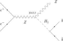
Figure 1: Higgs-boson production via Higgs-strahlung and subsequent decay into a $b\bar{b}$ quark pair, as searched for at the LEP experiment (Schael:2006cr, ). The coupling of the Higgs boson to the $Z$ bosons is denoted by $g_{HZZ}$ and given for the NMSSM in App. D.

But in the NMSSM the additional decay channel into a pair of pseudoscalar Higgs bosons, $H_{1}\rightarrow A_{1}A_{1}$, is open, reducing in general the $b\bar{b}$ decay-channel branching fraction. In the case $m_{A_{1}}<2m_{b}$, the subsequent decays of the pseudoscalar Higgs bosons can no longer proceed via b-quark pairs. In this case, the pseudoscalar decays into $\tau^{+}\tau^{-}$, $c\bar{c}$ or $gg$ and may escape detection. Then only the weaker decay mode independent LEP bound (Abbiendi:2002qp, )

$$m_{H_{1}}^{\text{(N)MSSM, exp}}>82~{}\text{GeV}$$ (58)

applies. This experimental search is not based on the decay products of the Higgs boson, but on the recoil mass spectrum of the Z boson in the process $e^{+}e^{-}\rightarrow ZH_{1}$. Therefore, the actual decay of the Higgs boson plays no role in this search and the given limit applies also to the NMSSM. To summarize, in the NMSSM we have a larger theoretical upper bound as well as a lower experimental bound and thus this model seems to be favored over the MSSM with respect to the Higgs-boson sector restrictions.

With these remarks on the restrictions in the Higgs-boson sector, let us also briefly comment on the approach of Barate et al., (Barate:2003sz, ), on Higgs-boson phenomenology in extensions of the SM. In Fig. 2 the upper limit on the ratio

$$\xi^{2}=\left(\frac{g_{\text{HZZ}}}{g_{\text{HZZ}}^{\text{SM}}}\right)^{2}$$ (59)

times the branching ratio $\operatorname{BR}(H\rightarrow b\bar{b})$ is shown, depending on the Higgs-boson mass. In this ratio $\xi^{2}$, the expression $g_{\text{HZZ}}^{\text{SM}}$ denotes the SM Higgs–Z–Z coupling, whereas $g_{\text{HZZ}}$ denotes the same non-standard coupling. The dark and bright bands give the 1–$\sigma$ and 2–$\sigma$ deviations from this limit. The limits on $\xi^{2}$ are gained from LEP1 data at the $Z$-resonance as well as from LEP2 data taken at energies between 161 and 209 GeV. The Higgs boson is assumed to decay into fermions and bosons according to the SM. The dominant decay channel in the SM proceeds via the $b\bar{b}$ channel. The Higgs-boson production cross sections for the processes $e^{+}e^{-}\rightarrow HZ$, $WW\rightarrow H$ and $ZZ\rightarrow H$ are scaled with the non-standard coupling squared $g_{\text{HZZ}}^{2}$. Obviously, the observation exceeds the upper limit for an assumed Higgs-boson mass of around 98 GeV.

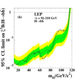
Figure 2: Upper limit on the ratio $\xi^{2}$ given in (59) times the branching ratio of the Higgs boson into $b\bar{b}$ according to the SM. The upper limit is gained from at LEP from LEP1 data at the $Z$ resonance as well as from LEP2 data taken at energies between 161 and 209 GeV. The dark and bright band give the 1–$\sigma$ and 2–$\sigma$ deviations from the central upper limit. The observation is shown (full line), exceeding the upper limit for a Higgs-boson mass of about 98 GeV. The horizontal line above represents the SM expectation on $\xi^{2}$. Figure taken from (Barate:2003sz, ).

As is argued in the works of Dermisek et al. (Dermisek:2005gg, ; Dermisek:2005ar, ), the observed excess is consistent with models which have a SM-like $ZZH_{1}$ coupling but a reduced branching ratio $\operatorname{BR}(H_{1}\rightarrow b\bar{b})$ due to new open decay channels. As aforementioned, in the NMSSM the light scalar Higgs boson may decay into a pair of pseudoscalars $H_{1}\rightarrow A_{1}A_{1}$. In case $m_{A_{1}}<2m_{b}$ the pseudoscalar $A_{1}$ can not subsequently decay into $b\bar{b}$ pairs, but decays into $\tau$ pairs or jets. As is argued, for a SM-like $ZZH_{1}$ coupling and $\operatorname{BR}(H_{1}\rightarrow b\bar{b})\approx 0.08$ and $\operatorname{BR}(H_{1}\rightarrow A_{1}A_{1})\approx 0.9$ the observed excess at $m_{H_{1}}\approx 98$ GeV is nicely reproduced.

Let us turn our attention to the prospects of Higgs-bosons in the NMSSM at the LHC, where we mention the approaches (Ellis:1988er, ; Gunion:1996fb, ; Rainwater:1998kj, ; Rainwater:1999sd, ; Yeghian:1999kr, ; Plehn:1999xi, ; Ellwanger:1999ji, ; Zeppenfeld:2000td, ; Kauer:2000hi, ; Dobrescu:2000jt, ; Ellwanger:2001iw, ; Ellwanger:2003jt, ; Ellwanger:2004gz, ; Dermisek:2005ar, ; Forshaw:2007ra, ).

In Ref. (Gunion:1996fb, ), published in 1996, the Higgs detection capability of LEP2 and LHC was studied. It was stated, that there is large parameter space, where all Higgs bosons in the NMSSM escape detection at both collider experiments, LEP2 and LHC. With respect to the LHC, an integrated luminosity as high as 600 fb^-1 was assumed.

However, in the meantime much improvements compared to the initial study could be achieved. In 2002 an investigation of Ellwanger, Gunion and Hugonie (Ellwanger:2001iw, ) was titled rather promising: Establishing a No-Lose Theorem for NMSSM Higgs Boson Discovery at the LHC. At this time there were improvements at the theoretical side, like the two-loop corrections to the effective potential (Yeghian:1999kr, ; Ellwanger:1999ji, ) and the predictions of the $W$-fusion channel Higgs-boson production at the LHC (Rainwater:1998kj, ; Rainwater:1999sd, ; Plehn:1999xi, ; Kauer:2000hi, ; Zeppenfeld:2000td, ). Moreover the improved LEP2 data were available, constraining the NMSSM parameter space further. Taking the newly predicted detection channels into account, that is the associated production of Higgs bosons with a top pair and the two $W$-fusion channel, altogether the following channel list is studied in (Ellwanger:2001iw, ):

$$\begin{split}1)\quad&gg\rightarrow H\rightarrow\gamma\gamma\,,\\ 2)\quad&WH\text{ or }t\bar{t}H\text{ production with }\gamma\gamma l^{\pm}\text{in the final state}\,,\\ 3)\quad&t\bar{t}H\text{ with }H\rightarrow b\bar{b}\,,\\ 4)\quad&gg\rightarrow H/A\text{ or }b\bar{b}H/A\text{ production with }H/A\rightarrow\tau\bar{\tau}\,,\\ 5)\quad&gg\rightarrow H\rightarrow ZZ^{*}\rightarrow 4\text{ leptons}\,,\\ 6)\quad&gg\rightarrow H\rightarrow WW^{*}\rightarrow l^{+}l^{-}\nu\bar{\nu}\,,\\ 7)\quad&\text{at LEP2: }e^{+}e^{-}\rightarrow ZH\text{ and }e^{+}e^{-}\rightarrow HA\,,\\ 8)\quad&WW\rightarrow H\rightarrow\tau\bar{\tau}\,,\\ 9)\quad&WW\rightarrow H\rightarrow WW^{*}\,,\end{split}$$ (60)

where $H$ denotes any CP-even and $A$ any CP-odd Higgs-boson, that is a CP-conserving Higgs-boson sector is considered. In this study, the Higgs–to–Higgs as well as Higgs–to–top decays are not taken into account, that is, parameter sets leading to a particle spectrum which allows kinematically for these decays are disregarded. Explicitely, the disregarded decay channels are $H\rightarrow HH$, $H\rightarrow AA$, $H\rightarrow H^{+}H^{-}$, $H\rightarrow AZ$, $A\rightarrow HA$, $A\rightarrow HZ$, $H/A\rightarrow H^{\pm}W^{\mp}$, $H/A\rightarrow t\bar{t}$, $t\rightarrow H^{+}b$. The suppression of these decay channels is implemented by invoking the following constraints:

$$\begin{split}m_{H_{3}}\;&<\;2m_{H_{1}},2m_{A_{1}},2m_{H^{\pm}},m_{A_{1}}+m_{Z},m_{H^{\pm}}+m_{W},\\ m_{A_{2}}\;&<\;m_{H_{1}}+m_{A_{1}},m_{H_{1}}+m_{Z},m_{H^{\pm}}+m_{W},\\ m_{H^{\pm}}&>\;155~{}GeV.\end{split}$$ (61)

Further assumptions are the absence of Landau singularities (see Sect. 5.1) and, as mentioned before, the LEP2 constraints on Higgs strahlung $e^{+}e^{-}\rightarrow ZH$ (:2001xwa, ) and $e^{+}e^{-}\rightarrow HA$ (:2001xx, ). Moreover, in the parameter space it is required that $|\mu|\equiv\lambda v_{s}>100$ GeV in order to avoid a light chargino, which is experimentally excluded. Neglecting kinematically the Higgs–to–Higgs, Higgs–to–top decays and Higgs–to–neutralino decays, it is found that at least one Higgs boson will be detected at LHC for a luminosity of 300 fb^-1 for arbitrary choices of remaining parameters, with a statistical discovery level of at least 5–$\sigma$.

In 2003 this investigation was followed by supplementing the missing $H\rightarrow AA$ decay channel via $W$-fusion, that is, $WW\rightarrow H\rightarrow AA$ (Ellwanger:2003jt, ) (Towards a no-lose theorem for NMSSM Higgs discovery at the LHC). There, special parameter sets are chosen, representing cases which are rather difficult for detection at the LHC in this channel due to difficulties with respect to the background.

In 2005 follows a study (Ellwanger:2005uu, ) (Difficult scenarios for NMSSM Higgs discovery at the LHC) with an investigation aiming to reveal parameter sets which yield a mass and coupling spectrum such that no Higgs boson is detectable at the LHC. A CP-conserving Higgs sector is considered. Gaugino mass unification is assumed, where $M_{2}=1$ TeV is fixed at the electroweak scale, corresponding to $M_{1}\approx 500$ GeV and $M_{\tilde{g}}\approx 3$ TeV. For the soft supersymmetry breaking parameters it is set $m_{Q}=m_{\tilde{u}}=m_{\tilde{d}}=m_{L}=m_{\tilde{e}}=1$ TeV for all three generations. Further, the $A$-parameters are fixed to $A_{u}=A_{d}=1.5$ TeV for all generations. Eventually, a minimal charged Higgs-boson mass, $m_{H^{\pm}}>155$ GeV, is assumed in order to avoid detection of charged Higgs bosons in decays like $t\rightarrow H^{\pm}b$ for moderate values of $\tan(\beta)$. This choice of parameters suggests that the Higgs-boson detection might be the only new signal at the LHC. Over the following ranges of remaining parameters is scanned:

$$10^{-4}\leq\lambda\leq 0.75\,,\quad-0.65\leq\kappa\leq 0.65\,,\quad 1.6\leq\tan(\beta)\leq 54\,,\quad-1\text{~{}TeV}\leq\mu=\lambda v_{s},A_{\lambda},A_{\kappa}\leq 1\text{~{}TeV}\,.$$ (62)

In this study the “no-lose” theorem is confirmed, if the Higgs-to-Higgs decays are kinematically excluded via (61). As is noted, this exclusion corresponds to large parts of available parameter space. In the complementary region of parameter space in deed parameters are found, where no detection at LHC may be achievable, as is reported. We repeat two example parameter sets, denoted by set 7 and 8,

parameter set	$\lambda$	$\kappa$	$\tan(\beta)$	$\mu$	$A_{\lambda}$	$A_{\kappa}$
7	0.5	-0.15	3.5	200	780	230
8	0.27	0.15	2.9	-753	312	8.4

which might lead to a particle and coupling spectrum not detectable at the LHC. In the parameter set 7 the next-to-lightest CP-even Higgs boson $H_{2}$ has SM-like couplings and decays dominantly via $H_{2}\rightarrow H_{1}H_{1}$, with branching ratio $\operatorname{BR}(H_{2}\rightarrow H_{1}H_{1})=0.93$. Moreover, the $H_{1}$ has only small couplings to $b\bar{b}$ and $\tau^{+}\tau^{-}$, following from the fact that $H_{1}$ is mostly $H_{u}^{0}$-like in the mixing matrix. This means that the signature $WW\rightarrow H_{2}\rightarrow 2j\;\tau^{+}\tau^{-}$ is suppressed and there remains only the $4j$ final state which is of course heavily plagued by QCD background. In parameter set 8 the lightest CP-even Higgs boson $H_{1}$ is SM-like and decays exclusively via $H_{1}\rightarrow A_{1}A_{1}$. In this scenario the pseudoscalar $A_{1}$ Higgs boson is very light, that is, $m_{A_{1}}=1$ GeV, and decays only into light jets. Thus, also this signature is overpowered by QCD background. The authors note that at a complementary $e^{+}e^{-}$ collider, like the proposed ILC, the scenarios, difficult to detect at the LHC, could be observed in the decay-independent signature $e^{+}e^{-}\rightarrow Z^{*}\rightarrow ZX$, as discussed in the end of this section.

In the work (Forshaw:2007ra, ) (Reinstating the ’no-lose’ theorem for NMSSM Higgs discovery at the LHC) a clear statement of a 5–$\sigma$ discovery of at least one Higgs boson is given. This statement is achieved by employing an additional constraint: it is argued that absence of large fine-tuning in the NMSSM corresponds to parameter space with a CP-even Higgs boson in the mass range $90\text{ GeV}<m_{H}<100\text{ GeV}$. In this work fine-tuning is studied on a quantitative basis, introduced later in Sect. 5.1. It is argued, that for a CP-even Higgs-boson with mass around 98 GeV, the only remaining decay not excluded by LEP may proceed via a light pair of pseudoscalars with subsequent decay into $\tau$’s or jets,

$$H\rightarrow AA\rightarrow\tau^{+}\tau^{-}\tau^{+}\tau^{-}\text{ or }4j\,.$$ (63)

The current experimental lower limits of this process with the decay into $\tau$’s is $m_{h}^{\text{NMSSM, exp}}>89$ GeV (Schael:2006cr, ) and with the decay into final state jets is $m_{h}^{\text{NMSSM, exp}}>82$ GeV (Abbiendi:2002qp, ) from the decay mode independent searches. This means that Higgs production with subsequent decay (63) is well beyond the constraints at LEP. Further, it is noted that the requirement $m_{A}<2m_{b}$ is natural in the sense of low fine-tuning. Nevertheless, it is found that this decay channel is very challenging to detect at the LHC in all so far studied Higgs production processes. However as an additional search strategy, the authors suggest to consider the well-known central exclusive production of a light Higgs boson $H$ via the process $pp\rightarrow ppH$. This process with the subsequent decay into a pair of pseudoscalar Higgs-bosons is shown in Fig. 3.

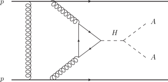
Figure 3: Central exclusive production of a light CP-even Higgs boson ($H$) in proton ($p$) collisions, $pp\rightarrow ppH$, as suggested by (Forshaw:2007ra, ). The Higgs boson $H$ decays into a pair of pseudoscalar Higgs bosons $A$. The process proceeds via a fermion loop.

This detection mode requires the outgoing protons $p$ to be detected in purpose-built low-angle detectors (FP420) (Cox:2004rv, ; Albrow:2005ig, ). Via these special detectors the four-momentum of the central system could be reconstructed very accurately and thus the masses of both the $H$ and the $A$ be determined on an event-by-event basis. The investigation shows that this technique in deed would allow for a discovery of the lightest Higgs bosons even when background is taken into account.

The decay chain (63) with $m_{A_{1}}<2m_{b}$ and large branching fractions $BR(A_{1}\rightarrow\tau^{+}\tau^{-})$ was also studied in the publication of Belyaev et al. (Belyaev:2008gj, ) in order to close the gap for a ’no-lose’ theorem. The parameters of the Higgs-boson sector (see Sect. 3.5) were varied in large ranges and the remaining parameters, which enter the Higgs-boson sector only at the suppressed loop level, were fixed in this study. The authors were looking for signatures, where two $\tau$’s decay into $\mu$’s and the other two $\tau$’s into jets. The Higgs-strahlung as well as the vector-boson-fusion production channels were considered and, as is reported, thousands of events are predicted, mostly originating from vector-boson-fusion processes. An extended investigation, taking also the background into account, is announced to be in preparation.

The decay channel with $A_{1}$ decaying into a pair of muons instead of taus has the advantage of much better detectability in the muon systems of the detector of hadron colliders. In Lisanti:2009uy it is reported that even for $2m_{\tau}<m_{A_{1}}<2m_{b}$, the subdominant decay into muons could be detected. Constraints were deduced recently from negative searches for the decay $H_{1}\rightarrow A_{1}A_{1}$ with either both pseudoscalars $A_{1}$ decaying to $\mu$’s or one decaying to $\mu$’s and the other to $\tau$’s by the D0 collaboration at Tevatron Abazov:2009yi . For the negative search for the four $\mu$ final state the upper limit of $\sigma(p\bar{p}\rightarrow H+X)\cdot\operatorname{BR}(H\rightarrow A_{1}A_{1})\cdot\operatorname{BR}(A_{1}\rightarrow\mu^{+}\mu^{-})^{2}\lesssim 10$ fb for $2m_{\mu}<m_{A_{1}}<2m_{\tau}$ is given. Note that the decay of even lighter pseudoscalars $m_{A_{1}}<2m_{\mu}$ is excluded by the model-independent search in proton–copper collisions at Nikhef Bergsma:1985qz .

Eventually we note that at a future electron–positron collider like the international linear collider (ILC) with center-of-mass energies up to 1 TeV, the study of the Higgs-strahlung process $e^{+}e^{-}\rightarrow Z^{*}\rightarrow ZH$ would be accessible for a large mass range of the Higgs bosons. In the ILC reference design report, referring to an investigation in the constrained NMSSM (Djouadi:2007ik, ), it is stated that the measurement of the Higgs-boson masses with a resolution of the order of 100 MeV could be achieved, if the Higgs bosons are not too heavy. A very direct approach available at an electron-positron collider is the Higgs-boson detection, independent on the subsequent decay-mode. From the recoil mass spectrum against the $Z$-boson in the process $e^{+}e^{-}\rightarrow Z^{*}\rightarrow ZX$ the Higgs boson is detectable if the couplings to the Z-boson are not too small. This decay-mode independent search is in particular interesting in the case, where the Higgs-to-Higgs decay is dominant and the LHC might fail to detect the decay products.

4 Neutralinos

The modification in the NMSSM compared to the minimal supersymmetric extension originates from the superpotential terms $\lambda\hat{S}(\hat{H}_{u}^{\mathrm{T}}\epsilon\hat{H}_{d})+\frac{1}{3}\kappa\hat{S}^{3}$ accompanied by the introduction of an additional singlet $\hat{S}$. Here we focus on the modification which arises from the fermionic part of the singlet $\hat{S}$, the so-called singlino $\tilde{S}$. For studies of the MSSM phenomenology we refer the reader to the review of Martin (Martin:1997ns, ) including detailed references. Note that we do not have additional charginos compared to the MSSM. The singlino component of the superfield gives a fifth neutralino which in general mixes with the bino $\tilde{B}^{0}$, wino $\tilde{W}^{0}$ and the Higgsinos $\tilde{H}_{d}^{0}$ and $\tilde{H}_{u}^{0}$; see Tab. 2. Collecting all quadratic terms as performed in App. D we arrive in the basis $\psi^{0}=(\tilde{B}^{0},\tilde{W}^{3},\tilde{H}_{d}^{0},\tilde{H}_{u}^{0},\tilde{S})^{\mathrm{T}}$ at the symmetric neutralino mass matrix

$$M_{\tilde{\chi}^{0}}=\begin{pmatrix}M_{1}&0&-c_{\beta}s_{W}m_{Z}&s_{\beta}s_{W}m_{Z}&0\\ 0&M_{2}&c_{\beta}c_{W}m_{Z}&-s_{\beta}c_{W}m_{Z}&0\\ -c_{\beta}s_{W}m_{Z}&c_{\beta}c_{W}m_{Z}&0&-\lambda v_{s}/\sqrt{2}&-\lambda v_{u}/\sqrt{2}\\ s_{\beta}s_{W}m_{Z}&-s_{\beta}c_{W}m_{Z}&-\lambda v_{s}/\sqrt{2}&0&-\lambda v_{d}/\sqrt{2}\\ 0&0&-\lambda v_{u}/\sqrt{2}&-\lambda v_{d}/\sqrt{2}&\phantom{+}\sqrt{2}\kappa v_{s}\end{pmatrix}.$$ (64)

This neutralino mass matrix reflects the fact that the singlino $\tilde{S}$ does not couple to the gauge bosons but only to the Higgsino doublets $\tilde{H}_{d}^{0}$, $\tilde{H}_{u}^{0}$ in addition to the selfcoupling in the lower diagonal entry. In case of a small mixing of the singlino with the Higgsinos the singlino decouples. In this case the behavior of the four neutralinos is MSSM-like and the mass of the singlino is at tree level given by the lower diagonal entry $m_{\tilde{S}}^{2}\approx 2\kappa^{2}v_{s}^{2}$. For large mass values $m_{\tilde{S}}$ the singlino may escape detection and a distinction of the NMSSM from the MSSM is very difficult (Choi:2004zx, ).

After diagonalization with the unitary rotation $U$ of the mass matrix (64) we end up with five neutralinos

$$\chi_{i}^{0}=U_{ji}\,\psi_{j}^{0}\,\qquad\text{with }i,j=1,...,5$$ (65)

which afterwards are arranged in ascending order, thus we end up in Dirac notation with $\tilde{\chi}_{i}^{0}$, $i=1,...,5$, with $\tilde{\chi}_{1}^{0}$ the lightest neutralino (more details are given in App. D). The singlino components of the mixed states do not couple to gauge bosons, gauginos, leptons, sleptons, quarks and squarks. Thus, in addition to an increased total number of neutralinos, we expect in particular a changed behavior compared to the MSSM for a neutralino with a large singlino component, that is for a singlino-like neutralino. It is worthwhile to note that the detection of a fifth neutralino would be a clear signal of an extended supersymmetric model. However, the production cross section of a singlino-like neutralino is rather small due to its small couplings. Moreover it is evident from its small couplings that a singlino-like neutralino, which is not the LSP, would be omitted in cascade decays.

In Fig. 4 the mass spectrum of the five neutralinos as well as the dominant mixings (couplings) of the mass eigenstates are shown depending on $\mu_{\lambda}\equiv\lambda v/\sqrt{2}$, as presented in (Choi:2004zx, ). The parameters chosen for this plot are given in the figure caption.

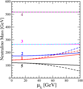
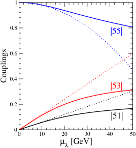
Figure 4: Neutralino masses (left) and mixings (right) depending on $\mu_{\lambda}\equiv\lambda v/\sqrt{2}$. The other parameters are fixed to $\sqrt{2}\kappa v_{s}=120$ GeV (this is the lower diagonal entry in the mixing matrix (64)), $M_{1}=250$ GeV, $M_{2}=500$ GeV, $\lambda v_{s}/\sqrt{2}=170$ GeV, $\tan(\beta)=3$. The numbering $i=1,...,5$ denotes the mass eigenstates in the mixing $\chi_{i}^{0}=U_{ji}\,\psi_{j}^{0}$ (65), before the arrangement in ascending order. The mixing entries in the matrix $U_{ji}$ are denoted in the right plot by the indices, that is, for instance $|53|$ denotes $|U_{53}|$. The dashed respectively dotted curves show an approximation, in case the singlino–Higgsino mixing is suppressed, that is, for $v\ll v_{s}$. Figure taken from (Choi:2004zx, ).

The parameter $\mu_{\lambda}$ determines the mixing of the singlino with the Higgsinos, as is evident from the mixing matrix (64). We see that in this scenario the lightest neutralino is singlino-like, since the mixing $U_{55}$ is dominant for small values of $\mu_{\lambda}$ as shown on the right hand side of Fig. 4. This is what is expected since for small $\mu_{\lambda}$ the singlino decouples from the other neutralinos. Let us note that in (Choi:2004zx, ) a study of neutralino production cross sections in $e^{+}e^{-}$ collisions and decay rates of the neutralinos can also be found.

In the study by Hesselbach and Franke (Hesselbach:2002nv, ) the associated singlino-like neutralino production is discussed

$$e^{+}e^{-}\rightarrow\tilde{\chi}_{1}^{0}\tilde{\chi}_{S}^{0}\,,$$ (66)

where $\tilde{\chi}_{S}^{0}$ denotes a singlino-like neutralino. From the neutralino mixing matrix (64) we see from the lower diagonal entry that we get a neutralino with a large singlino component for a large vacuum-expectation-value $v_{s}$.

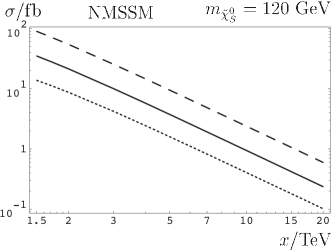
Figure 5: Total cross section for singlino-like neutralino production $e^{+}e^{-}\rightarrow\tilde{\chi}_{1}^{0}\tilde{\chi}_{S}^{0}$ depending on the vacuum-expectation-value $v_{s}$, here denoted by $x$ as presented by Hesselbach and Franke (Hesselbach:2002nv, ). The electron–positron center-of-mass energy is fixed to 500 GeV. The model parameters chosen are inspired by the SPS1a scenario in the MSSM with $M_{1}=99$ GeV, $M_{2}=193$ GeV, $\tan(\beta)=10$, $\mu=\lambda v_{s}=352$ GeV. The full line refers to unpolarized beams, the dashed line to beam polarizations $P_{-}=+0.8$, $P_{+}=-0.6$ and the dotted line to beam polarizations $P_{-}=-0.8$, $P_{+}=+0.6$. The mass of the neutralino $\tilde{\chi}_{S}^{0}$ is fixed at 120 GeV by the $\kappa$-parameter.

As shown in Fig. 5 the total cross section drops with increasing singlet vacuum-expectation-value $v_{s}$ (denoted by $x$ in this work), as is evident from the increasing singlino-component in $\tilde{\chi}_{S}^{0}$, that is, smaller couplings for rising $v_{s}$. The effect of beam polarization is also shown in this figure and we see that we get total cross sections of the order of 10 femtobarn for not too large $v_{s}$, depending also on the beam polarizations. The chosen parameters in this example are given in the figure caption.

In case that four light neutralinos are detected, the distinction of the minimal supersymmetric model from further extension is in general difficult. As noted already, a heavy singlino-like neutralino would be omitted in cascade decays of even heavier supersymmetric partner particles. In case there is substantial mixing in the neutralino sector there is a method discussed by Choi et al. (Choi:2001ww, ) to discriminate the NMSSM from the MSSM at a future electron–positron collider: the total cross section, summed over the four light neutralinos and normalized to its asymptotic form in the limit of infinite center-of-mass energies, is sensitive to the total number of neutralinos.

Figure 6: Energy dependence of the four light neutralino production cross sections summed up and normalized to its asymptotic form for infinite center-of-mass energies. The full line corresponds to the MSSM, whereas the dashed line corresponds to the NMSSM. The assumed parameters are $\tan(\beta)=10$, $|M_{1}|=100.5$ GeV, $M_{2}=190.8$ GeV, $|\mu|=|\lambda v_{s}|=365.1$ GeV where CP-invariance in the Higgs-boson sector is assumed. The selectron masses are fixed to $m_{\tilde{e}_{L}}=208.7$ GeV and $m_{\tilde{e}_{R}}=144.1$ GeV. Figure taken from (Choi:2001ww, ).

The energy dependence of the ratios for the MSSM and the NMSSM is shown in Fig. 6. The model parameters chosen in this plot are given in the figure caption.

There remains the possibility that the singlino-like neutralino is the LSP as discussed in more detail in Sect. 5.4. Parameter scans in the NMSSM show that there is indeed large parameter space with this possibility passing all nowadays known theoretical and experimental constraints. Due to conserved matter parity this LSP singlino-like neutralino would escape detection. However, due to its small couplings, the next-to-lightest supersymmetric particle (NLSP) would decay very slowly into the singlino-like LSP. This opens the possibility to observe displaced vertices (Ellwanger:1997jj, ; Ellwanger:1998vi, ; Hesselbach:2000qw, ). The partial decay width of a sfermion $\tilde{f}$ decaying into the LSP neutralino $\tilde{\chi}_{1}^{0}$ and a fermion $f$ is (Bartl:1996wt, ; Kraml:2005nx, ; Djouadi:2008uj, )

$$\Gamma(\tilde{f}\rightarrow\tilde{\chi}_{1}^{0}f)=\frac{\rho^{1/2}(m_{\tilde{f}},m_{\tilde{\chi}_{1}^{0}},m_{f})}{16\pi m_{\tilde{f}}^{3}}\left((a^{2}+b^{2})(m_{\tilde{f}}-m_{\tilde{\chi}_{1}^{0}}-m_{f})-4\;a\;b\;m_{\tilde{f}}m_{\tilde{\chi}_{1}^{0}}\right)$$ (67)

with kinematic function $\rho(x,y,z)=x^{2}+y^{2}+z^{2}-2xy-2xz-2yz$ and $a$ and $b$ the left- and right couplings in the Lagrangian

$${\cal L}_{\tilde{f}f\tilde{\chi}_{1}^{0}}=\bar{f}(aP_{R}+bP_{L})\tilde{\chi}_{1}^{0}\tilde{f}+c.c.$$ (68)

The length of flight of the sfermion is simply $l_{\tilde{f}}=\hbar c/\Gamma(\tilde{f}\rightarrow\tilde{\chi}_{1}^{0}f)$. Scenarios of the NMSSM are studied for which a NLSP $\tilde{\chi}_{2}^{0}$ decays into a singlino-like LSP $\tilde{\chi}_{1}^{0}$. As is pointed out, rather large vacuum-expectation-values $v_{s}$ are required in order to get a very pure singlino-like neutralino and suppressed couplings accompanied by observable displaced vertices.

In the approach of Kraml, Raklev and White (Kraml:2008zr, ) a special scenario is studied, motivated by the parameter set SPS1a in the MSSM and extended to the NMSSM. In this scenario, the LSP is a singlino-like neutralino $\tilde{\chi}_{1}^{0}$ and the NLSP a bino-like neutralino $\tilde{\chi}_{2}^{0}$ with a small mass difference $\Delta m=m_{\tilde{\chi}_{2}^{0}}-m_{\tilde{\chi}_{1}^{0}}$. Their analysis is based on cascade decays which eventually end up with the decay

$$\tilde{\chi}_{2}^{0}\rightarrow\tilde{\chi}_{1}^{0}\,l^{+}\,l^{-}\,.$$ (69)

Due to the small mass difference, the final state leptons are soft and could escape detection. As the authors emphasize, with a typical kinematical cut on the minimal transversal momentum of leptons at the LHC this could lead to a wrong interpretation of a $\tilde{\chi}_{2}^{0}$ LSP, since non of the true final state particles would be seen in this case. Accepting low momenta of the final state leptons, the measurement of the invariant di-lepton mass squared distribution $m_{ll}^{2}\equiv(p_{l}^{+}+p_{l}^{-})^{2}$, with the momenta of the leptons denoted with $p_{l}^{\pm}$, would allow to determine the mass difference $\Delta m=m_{\tilde{\chi}_{2}^{0}}-m_{\tilde{\chi}_{1}^{0}}$ at the edge of a measured $m_{ll}^{2}$ distribution.

5 Parameter constraints

In this section we will discuss some parameter constraint studies, performed in the NMSSM. We start with theoretical constraints. Constraints originating from a viable global minimum of the Higgs potential, that is, a global minimum which has the correct electroweak symmetry breaking behavior, are discussed in detail in Sect. 6. We mention the requirement of perturbativity of couplings in considering renormalization group equations. Then we turn to fine-tuning. In a series of recent papers some attention is payed to fine-tuning in extensions of the SM; for instance in (Dermisek:2005ar, ; Dermisek:2005gg, ; Dermisek:2008uu, ), where fine-tuning is quantified in terms of a simple function. We proceed with constraints coming from the requirement of a vacuum which does not break color- and electric charge. Also an approximative constraint can be gained from the condition to have a non-vanishing vacuum-expectation-value for the singlet $\langle S\rangle=v_{s}$. On the experimental side we first consider the firm exclusion limits from collider experiments. Further constraints with respect to the anomalous magnetic moment of the muon, the b-meson decay, cosmological constraints from indirect as well as direct detection of cold dark matter and strong first order electroweak phase transitions are considered. Finally, we review some generic parameter scans over large parameter regions, revealing the viable parameter space.

5.1 Theoretical constraints

Let us start with the Landau pole exclusion constraint. The renormalization group equations for the NMSSM have been determined to two-loop order. Here we present the one-loop results of the gauge couplings and the superpotential parameters $\lambda$ and $\kappa$ as well as $y_{t}$ in the case of a CP-conserving Higgs sector (Miller:2003ay, ).

$$\begin{split}\frac{\operatorname{d}}{\operatorname{d}t}\bar{g}_{a}=&\frac{1}{16\pi^{2}}\;\frac{b_{a}}{2}\bar{g}_{a}^{3},\qquad(a=1,2,3)\;,\\ \frac{\operatorname{d}}{\operatorname{d}t}y_{t}^{2}=&\frac{1}{16\pi^{2}}\;y_{t}^{2}\left(\lambda^{2}+6y_{t}^{2}-\frac{16}{3}\bar{g}_{3}^{2}-\frac{13}{15}\bar{g}_{1}^{2}\right)\;,\\ \frac{\operatorname{d}}{\operatorname{d}t}\lambda^{2}=&\frac{1}{16\pi^{2}}\;\lambda^{2}\left(4\lambda^{2}+2\kappa^{2}+3y_{t}^{2}-3\bar{g}_{2}^{2}-\frac{3}{5}\bar{g}_{1}^{2}\right)\;,\\ \frac{\operatorname{d}}{\operatorname{d}t}\kappa^{2}=&\frac{1}{16\pi^{2}}\;6\kappa^{2}\left(\lambda^{2}+\kappa^{2}\right)\;.\end{split}$$ (70)

The coefficient for the couplings are $b_{1}=33/5$, $b_{2}=1$, $b_{3}=-3$. The context of the gauge couplings $\bar{g}_{1}$, $\bar{g}_{2}$ with the conventional couplings is $\bar{g}_{1}=\sqrt{5/3}g_{1}$, $\bar{g}_{2}=g_{2}$ with, as usual, $e=g_{2}\sin(\theta_{W})=g_{1}\cos(\theta_{W})$. The scale factor is defined as $t=\ln(Q^{2}/m_{\text{GUT}})$ with unification scale $m_{\text{GUT}}\approx 3\cdot 10^{16}$ GeV and $Q$ the scale under consideration. Note that the unification of the gauge couplings at the GUT scale occurs also in the NMSSM, like in the MSSM. This is due to the fact, that the additional superfield $\hat{S}$ is a gauge-singlet.

The requirement of perturbativity of the couplings means that quantum corrections are assumed not to become too large at all scales from the electroweak scale of about $100$ GeV up to the gand unification scale of about $3\cdot 10^{16}$ GeV (typically, the couplings are required not to exceed $2\pi$). At least there should not be any Landau pole for the couplings. Due to the $\beta$ functions given in (70) we see that $\lambda$ and $\kappa$ drop with a decreasing energy scale $t$. That is, perturbativity up to the GUT scale gives a strong constraint of these coupling parameters at the electroweak scale. As an example, in Fig. 7 the running of the couplings $\lambda$ and $\kappa$ with the assumption of real parameter values is shown.

Figure 7: Evolution of the dimensionless NMSSM parameters $\lambda$ and $\kappa$ supposed to be real (Miller:2003ay, ). The Yukawa coupling $h_{t}$ is set to $0.8$ at the grand unification scale, $Q_{\text{GUT}}=3\cdot 10^{16}$ GeV. For the evolution of $\lambda$ we start with $\lambda(Q_{\text{GUT}})=3$ and $\kappa(Q_{\text{GUT}})=1$. The evolution of $\kappa$ is given for vice versa values, that is $\kappa(Q_{\text{GUT}})=3$ and $\lambda(Q_{\text{GUT}})=1$. See (Miller:2003ay, ) for more details.

It is worthwhile to note, that the constraint of perturbativity up to the GUT or Planck scale is based on the assumption, that the NMSSM is valid up to the very high GUT or Planck scale. In spite of the unification of gauge couplings, which indicate that this could be true, this is not granted even if the NMSSM may be correct as an effective theory at the electroweak scale.

One of the main motivations for the introduction of supersymmetry is to avoid the fine-tuning problem we encounter in the SM. that is, we expect the model under consideration not to reintroduce fine-tuning again. In order to quantify fine-tuning an appropriate quantity is introduces (Barbieri:1987fn, ),

$$F=\mathop{\max}_{a_{i}}\left|\frac{\operatorname{d}\ln(m_{Z}(a_{i}))}{\operatorname{d}\ln(a_{i})}\right|\,,$$ (71)

with $a_{i}$ denoting all soft supersymmetry breaking parameters. Note, that in the original work the $Z$-boson mass occurs squared in this expression. With help of this quantity $F$, parameter sets within a certain model may be compared on a quantitative basis and the parameters giving lower values of $F$ correspond to a more natural parameter choice. Moreover this allows also for a comparison of different models with respect to fine-tuning. This approach is employed in some studies on the Higgs-boson spectrum in the NMSSM; see Sect. 5.4.

A further restriction for the parameters in the potential comes from the requirement of a color and electric charge-invariant vacuum (Frere:1983ag, ; Gunion:1987qv, ). This is evident if we consider for instance the scalar part of the slepton–slepton–Higgs superpotential term $-{\tilde{e}_{R}^{*}}y_{e}(\tilde{L}^{\mathrm{T}}\epsilon H_{d})$; see (5). With view on Tab. 1 we see that the supermultiplets have hypercharges $Y(\tilde{e}_{R})=1$, $Y(\tilde{L})=-1/2$ and $Y(H_{d})=-1/2$ and thus, the superpotential term is invariant under $U_{Y}(1)$ transformations. However a non-zero vacuum-expectation-value of the scalar field $\tilde{e}_{R}$ corresponds to a electric charge breaking minimum. In a analogous way also color breaking minima may arise from the potential. The undesired global minima of the scalar fields can be translated into charge- and color-breaking bounds (CCB). Let us sketch the bounds found on the $A$-parameter, where we follow closely (Gunion:1987qv, ). We start with a generic trilinear superpotential term $W_{\phi}=\lambda\hat{\phi}_{1}\hat{\phi}_{2}\hat{\phi}_{3}$ with a corresponding scalar part $W_{\phi}=\lambda\phi_{1}\phi_{2}\phi_{3}$. As shown in App. C we get from this superpotential term a physical potential by collecting the F-terms, D-terms as well as the corresponding soft supersymmetry breaking terms, yielding mass terms and trilinear $A$-parameter terms. The physical potential thus reads

$$\begin{split}V_{\phi}(\phi_{1},\phi_{2},\phi_{3})=&|\lambda|^{2}\left(|\phi_{1}|^{2}|\phi_{2}|^{2}+|\phi_{2}|^{2}|\phi_{3}|^{2}+|\phi_{1}|^{2}|\phi_{3}|^{2}\right)\\ &+g_{a}^{2}\left(Y_{\phi_{1}}^{a}|\phi_{1}|^{2}+Y_{\phi_{2}}^{a}|\phi_{2}|^{2}+Y_{\phi_{3}}^{a}|\phi_{3}|^{2}\right)^{2}\\ &+m_{\phi_{1}}^{2}|\phi_{1}|^{2}+m_{\phi_{2}}^{2}|\phi_{2}|^{2}+m_{\phi_{3}}^{2}|\phi_{3}|^{2}\\ &+\left(A\lambda\phi_{1}\phi_{2}\phi_{3}+c.c.\right)\,.\end{split}$$ (72)

Here we denote by $Y_{\phi_{i}}^{a}$, $i=1,2,3$ the eigenvalues of the gauge group generators with adjoint index $a$ and corresponding couplings $g_{a}$, originating from the D-terms. Since the initial superpotential term (along with its derived Lagrangian terms) is supposed to be gauge invariant we have to have $Y_{\phi_{3}}^{a}=-(Y_{\phi_{1}}^{a}+Y_{\phi_{2}}^{a})$. Now we are looking for the global minimum of the potential $V_{\phi}$. To this end we examine the directions in field space with $\phi\equiv\phi_{1}=\phi_{2}=\phi_{3}$. In this direction in field space, the so-called D-flat direction, the quartic D-terms of the potential vanish, and do not protect the potential from a stationary solution for non-vanishing fields. Moreover, in the D-flat direction the potential becomes very simple, that is

$$V_{\phi}(\phi)=3|\lambda|^{2}|\phi|^{4}+\left(m_{\phi_{1}}^{2}+m_{\phi_{2}}^{2}+m_{\phi_{3}}^{2}\right)|\phi|^{2}-2A\lambda\phi^{3}\,.$$ (73)

Of course we have the desired stationary solution for $\phi=0$ with $V_{\phi}(0)=0$. In order to avoid a vacuum for non-vanishing fields and thus to avoid a charge breaking minimum, there has not to be a stationary solution with a negative potential value. This eventually restricts the $A$-parameter not to be too large, that is we find the constraint

$$A^{2}<3\left(m_{\phi_{1}}^{2}+m_{\phi_{2}}^{2}+m_{\phi_{3}}^{2}\right)\,.$$ (74)

A further approximative constraint arises from the Higgs potential with respect to the Higgs singlet (Frere:1983ag, ; Gunion:1987qv, ; Djouadi:2008uj, ). The dominant singlet-dependent part of the Higgs potential (26) reads

$$V_{S}(S)=\kappa^{2}S^{4}+\frac{2}{3}\kappa A_{\kappa}S^{3}+m_{S}^{2}S^{2}+...\;,$$ (75)

where the ellipsis denote terms which have a lower dependence on $S$. Generally, we want to have a non-vanishing $\mu$-term, with $\mu=\lambda v_{s}$, requiring a non-vanishing vacuum-expectation-value $v_{s}$. That is, in this case we have to have a minimum with a lower potential value compared to the symmetric minimum at $V_{S}(0)\approx 0$. This immediately translates into the approximate parameter condition

$$m_{S}^{2}\lesssim\frac{1}{9}A_{\kappa}^{2}\,.$$ (76)

Note, that this relation is only approximatively valid, since terms in the potential (75) are neglected.

In (Miller:2003ay, ) the impact of the vacuum stability constraints as well as the experimental constraints on the Higgs-boson sector parameter space is studied. Simple analytic expressions for the physical Higgs masses in the CP-conserving case are derived, taking the one-loop contributions to the Higgs-boson masses from top and stop loops into account. Using a power expansion in both $1/\tan(\beta)$ and $1/M_{A}$, where $M_{A}$ is the upper left entry in the pseudoscalar mass squared matrix (45), analytic expressions are found, approximative valid for moderate or large values of $\tan(\beta)$ and a larger scale $M_{A}$. Three distinct regions are considered with respect to the PQ-symmetry breaking parameter $\kappa$. The region with vanishing $\kappa$ corresponds to the PQ-symmetric NMSSM, the region with large values of $\kappa$, denoted as the NMSSM with strongly broken PQ-symmetry and the region with small values of $\kappa$, that is, $\kappa\ll 1$, denoted as slightly broken PQ-symmetry. Of course, the negative searches for a light axion on the one hand and the requirement of absence of a Landau-pole through renormalization group equations for $\kappa$ up to the GUT scale favor the slightly broken PQ-symmetry scenario (see Sect. 5.1). As an example, the Higgs-boson masses are plotted in a slightly broken PQ-symmetry scenario, namely with $\kappa=0.1$ in Fig. 8. The other parameters choices are given in the figure caption. Also the strong experimental constraint on the $m_{A}$ parameter is indicated in this figure. Note, that $m_{A}$ in general is not a CP-odd Higgs boson mass in the NMSSM, but the upper left entry in pseudoscalar mixing matrix squared; see (46).

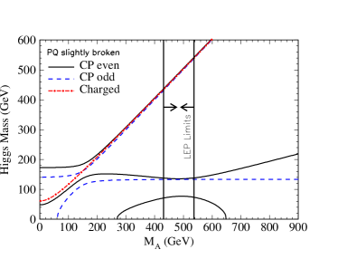
Figure 8: The one-loop Higgs-boson mass spectrum as a function of $M_{A}$, the upper left entry in the CP-odd mixing matrix. The remaining parameters are fixed to $\kappa=0.1$, depicted as slightly broken PQ-symmetry, $v_{s}=3v$, $\tan(\beta)=3$ and $A_{\kappa}=-100$ GeV. The arrows denote the region allowed by LEP searches with 95% confidence. Figure taken from (Miller:2003ay, ).

The authors point out, that the spectrum, based on their assumptions, in the NMSSM is quite different from what is to expect from the MSSM. So, even if some of the Higgs bosons are too heavy to be detected, the discovery of the lighter Higgs-bosons may allow to distinguish the NMSSM from the MSSM.

5.2 Experimental constraints

5.2.1 Collider constraints

The collider constraints give very clear bounds originating from very different observations like the Z-boson width as well as the direct searches of supersymmetric partner particles in $e^{+}e^{-}$ collisions at LEP. Here we discuss the bounds which are applied in the NMHDECAY program (Ellwanger:2004xm, ; Ellwanger:2005dv, ); see App. B for an overview of some currently available program tools with respect to the NMSSM.

A strong constraint arises form the Z-boson precision measurements at LEP (Amsler:2008zzb, ). A possible contribution for the decay into the lightest and stable neutralino pairs $Z\rightarrow\tilde{\chi}^{0}_{1}\tilde{\chi}^{0}_{1}$ with mass $m_{\tilde{\chi}^{0}_{1}}<m_{Z}/2$ may spoil the measurement of the invisible decay width $\Gamma_{Z}^{\text{invisible}}\equiv\Gamma_{Z}^{\text{tot}}-\Gamma_{Z}^{\text{visible}}$. From a resonance scan the total width $\Gamma_{Z}^{\text{tot}}=2.4952\pm 0.0023$ GeV (along with the Z-boson mass, $m_{Z}=91.1876\pm 0.0021$ GeV) is known. The visible decay width consists of decays into charged leptons ($\Gamma_{Z}^{l^{+}l^{-}}=83.984\pm 0.086$ MeV, with $l=e,\mu,\tau$) and hadrons ($\Gamma_{Z}^{\text{had}}=1744.4\pm 2.0$ MeV). From this the invisible decay width is measured as $\Gamma_{Z}^{\text{invisible}}=499.0\pm 1.5$ MeV. This is about what we expect from the SM, which predicts an invisible part, consisting solely of neutrinos as $\Gamma_{Z}^{\text{invisible, SM}}=501.3\pm 0.6$ MeV. This means a possible contribution of decays into neutralinos should not exceed the measurement too much,

$$\Gamma(Z\rightarrow\tilde{\chi}^{0}_{1}\tilde{\chi}^{0}_{1})\lesssim 2~{}\text{MeV}\,.$$ (77)

Neutralinos may be produced in pairs at LEP via s-channel Z-boson or Z-boson $\gamma$ interference or via t-channel exchange of a selectron. A further constraint arises from searches for pair production of non-LSP neutralinos with subsequent decay. These processes were searched for at LEP up to center-of-mass energies of 208 GeV (Abdallah:2003xe, ). From this negative search results the limits on the cross sections

$$\begin{split}\sigma(e^{+}e^{-}\rightarrow\tilde{\chi}_{1}^{0}\tilde{\chi}_{i}^{0})&<0.01~{}\text{pb}\,,\\ \sigma(e^{+}e^{-}\rightarrow\tilde{\chi}_{i}^{0}\tilde{\chi}_{j}^{0})&<0.1~{}\text{pb}\end{split}$$ (78)

with $i,j=2,...,5$ can be deduced, viable for a sum of neutralino masses in the final state not exceeding the center-of-mass energy of the colliding electrons.

Charginos could have been produced in pairs at LEP via s-channel exchange or via t-channel exchange of a sneutrino. The negative search can be translated into a minimal chargino mass limit of (lepsusywg, )

$$m_{\tilde{\chi}^{\pm}}>103.5~{}\text{GeV}\,.$$ (79)

The production of charged Higgs bosons in pairs $e^{+}e^{-}\rightarrow H^{+}H^{-}$ was investigated at LEP (:2001xy, ) for general SM extensions with two Higgs doublets, like the MSSM or the NMSSM. Assuming main decay channels of the charged Higgs bosons $H^{+}\rightarrow c\bar{s}$ and $H^{+}\rightarrow\tau^{+}\nu_{\tau}$ and charged conjugated decay products for the $H^{-}$, a combination of all four LEP experiments ALEPH, DELPHI, L3 and OPAL with center-of-mass energies up to 209 GeV, give a lower mass limit of

$$m_{H^{\pm}}>78.6~{}\text{GeV}\,.$$ (80)

There are constraints from the negative searches of the lightest CP-even Higgs boson $H_{1}$ based on CP-conserving NMSSM Higgs sector studies. The dominant production at LEP proceeds via Higgs-strahlung off a s-channel $Z$-boson ($e^{+}e^{-}\rightarrow Z^{*}\rightarrow ZH$). This Higgs-boson production channel was searched for in various subsequent decay channels. The bounds derived in this way depend on the Higgs-boson mass. Here we mention the subsequent decays $H\rightarrow b\bar{b}$ and $H\rightarrow\tau^{+}\tau^{-}$ (Barate:2003sz, ), $H\rightarrow jj$, with $j$ denoting a jet (:2001yb, ; Abbiendi:2003gd, ), $H\rightarrow\gamma\gamma$ (lephwg, ), $H\rightarrow$ invisible, that is, into LSP neutralinos (Buskulic:1993gi, ; :2001xz, ), $H\rightarrow X$, that is, independent of the decay product $X$ in $e^{+}e^{-}\rightarrow ZX$. The latter channel is accessible by studying the recoil mass spectrum in $Z\rightarrow e^{+}e^{-}$ and $Z\rightarrow\mu^{+}\mu^{-}$ events and by searching for $X\rightarrow e^{+}e^{-}$ or $X\rightarrow\gamma\gamma$ and $Z\rightarrow\nu\bar{\nu}$ (Buskulic:1993gi, ; Abbiendi:2002qp, ), $H\rightarrow AA$ with subsequent decay $AA\rightarrow 4j$, $AA\rightarrow 2j\,c\bar{c}$, $AA\rightarrow 2j\,\tau^{+}\tau^{-}$, $AA\rightarrow\tau^{+}\tau^{-}\tau^{+}\tau^{-}$, $AA\rightarrow c\bar{c}c\bar{c}$, $AA\rightarrow\tau^{+}\tau^{-}c\bar{c}$ (Abbiendi:2002in, ). Also it was looked for the associated production of two Higgs bosons, $e^{+}e^{-}\rightarrow HA$, with subsequent decay $HA\rightarrow b\bar{b}b\bar{b}$, $HA\rightarrow\tau^{+}\tau^{-}\tau^{+}\tau^{-}$, and $HA\rightarrow AAA\rightarrow 3(b\bar{b})$ (Abdallah:2004wy, ).

5.2.2 Muon anomalous magnetic moment

The muon anomalous magnetic moment is a quantum effect which is very valuable in studying the possible deviations from the SM. For a recent review we refer the reader to Stöckinger (Stockinger:2006zn, ).

The magnetic moment of an electron or muon is

$$\boldsymbol{\mu}=g\bigg{(}\frac{e}{2m}\bigg{)}\boldsymbol{s}$$ (81)

with $m$ mass, $e$ charge, and $\boldsymbol{s}$ spin of the electron or muon and $g$ the gyromagnetic ratio, which is $g=2$ following from the Dirac equation at the classical level. Quantum effects lead to a deviation from this value, called the anomalous magnetic moment

$$a\equiv\frac{1}{2}(g-2)\,.$$ (82)

The one-loop QED correction was first calculated by Schwinger and is $a=\frac{\alpha}{2\pi}$ (Schwinger:1948iu, ).

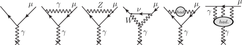
Figure 9: Contributions to the muon magnetic moment. From left to right the first diagram gives the contribution to the normal gyromagnetic ratio $g=2$. The deviations to $g=2$, that is the anomalous magnetic moment come from the quantum corrections shown in the five right diagrams. The second diagram gives the leading QED Schwinger contributing $\frac{\alpha}{2\pi}$ to $a$ in (82), the third and forth diagrams are the leading electroweak contributions. The fifth diagram shows the leading hadronic contribution via vacuum polarization and the last one the hadronic light-by-light contribution; see the review (Stockinger:2006zn, ).

The contributions to the muon magnetic moment are shown in Fig 9. Generally, loop contribution from heavy particles with mass $M$ are suppressed by a factor $m^{2}/M^{2}$ (Stockinger:2006zn, ). This makes clear that the anomalous magnetic moment of the muon, $a_{\mu}$, is enhanced by a factor $(m_{\mu}/m_{e})^{2}\approx 40,000$ compared to the electron with respect to these contributions.

For a muon anomalous magnetic moment calculation in the SM we refer to the more recent publications mentioned by the Particle Data Group, (Davier:2002dy, ; Davier:2003pw, ; deTroconiz:2004tr, ; Hagiwara:2006jt, ; Davier:2007ua, ; Jegerlehner:2007xe, ). For the corresponding calculation of the muon anomalous magnetic moment in SUSY models see (Lopez:1993vi, ; Chattopadhyay:1995ae, ; Moroi:1995yh, ; Carena:1996qa, ; Stockinger:2006zn, ; Hertzog:2007hz, ; Marchetti:2008hw, ).

Let us briefly present the current results. The Brookhaven $g-2$ experiment E821 (Bennett:2004pv, ; Bennett:2006fi, ) measures an anomalous magnetic moment of the muon of

$$a^{\text{exp}}_{\mu}=(116,592,080\pm 63)\times 10^{-11}$$ (83)

compared to the prediction of the SM, see the review (Miller:2007kk, ),

$$a^{SM}_{\mu}=(116,591,785\pm 61)\times 10^{-11}\,.$$ (84)

Thus we get a deviation of

$$\delta a_{\mu}=a^{\text{exp}}_{\mu}-a^{SM}_{\mu}=(295\pm 88)\times 10^{-11}\,,$$ (85)

where we added the errors quadratically. If we trust the measurement as well as the SM prediction, this is a more than 3–$\sigma$ deviation. The situation is presented by the Particle Data Group (Amsler:2008zzb, ) and displayed in Fig. 10. In this figure the deviations of the predictions from the BNL measurement are shown. Note that the prediction based on the $\tau$ data which enter the hadronic vacuum polarization contribution do not deviate very much from the measurement, whereas all other predictions based on $e^{+}e^{-}$ data show a large deviation.

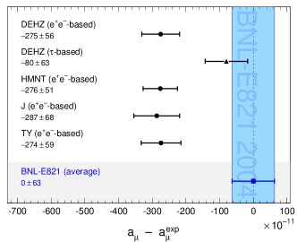
Figure 10: Recently published predictions of the SM anomalous magnetic moment of the muon $a_{\mu}$, subtracted from the mean experimental value from Brookhaven E821, as presented by the Particle Data Group (Amsler:2008zzb, ). The dots are predictions based on $e^{+}e^{-}$ data, the small triangle the prediction based on $\tau$ data and the experimental measurement is given by a little square. The predictions are taken from (Davier:2002dy, ; Davier:2003pw, ; deTroconiz:2004tr, ; Hagiwara:2006jt, ; Davier:2007ua, ; Jegerlehner:2007xe, ).

With an E821 upgrade proposal, called E969 (LeeRoberts:2005uy, ), the error is aimed to be at least halved and with the same improvement of the theoretical predictions (Miller:2007kk, ), the 5–$\sigma$ discovery limit may in principle be reached.

Of course supersymmetry changes the predictions of $a_{\mu}$, since we get also quantum correction contributions from the superpartners. The outcome depends on the masses and couplings, not to mention the supersymmetric model under consideration itself. In any case, the experimental result (83) gives a strong constraint on the model. Additional Feynman diagrams to lowest order contributing to the anomalous magnetic moment $a_{\mu}$ in the MSSM and the NMSSM are shown in Fig. 11.

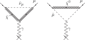
Figure 11: Additional Feynman diagrams contributing to the anomalous magnetic moment of the muon $a_{\mu}$ in the MSSM and the NMSSM.

For large $\tan(\beta)$ the dominant supersymmetric contribution comes from the chargino–sneutrino loop diagram and is approximately given by (Czarnecki:2001pv, )

$$|\delta a_{\mu}^{\text{SUSY}}|\approx\frac{\alpha}{8\pi s_{W}^{2}}\frac{m_{\mu}^{2}}{\tilde{M}^{2}}\tan(\beta)\;\left(1-\frac{4\alpha}{\pi}\ln\left(\frac{\tilde{M}}{m_{\mu}}\right)\right)\;,$$ (86)

with $\alpha$ the fine structure constant and $\tilde{M}$ the heavier of the masses in the loop, that is, either the mass of the chargino or the sneutrino.

The additional contribution to $a_{\mu}$ in the constrained NMSSM (cNMSSM) (The cNMSSM is introduced in App. E) is shown in Fig. 12 in dependence on the unified gaugino mass $M_{1/2}$, where the unified scalar mass $m_{0}$ is fixed to zero (Djouadi:2008uj, ). We see in this plot that the cNMSSM gives for $M_{1/2}\lesssim 1$ TeV a contribution in agreement with the observation at BNL.

It is worthwhile to add some critical remarks: first of all the experimental value with this high precision of ($0.54$ ppm) is not confirmed by an alternative laboratory. Secondly, the uncertainty of the predictions is obvious from the deviating results based on the one hand on $e^{+}e^{-}$ data and on the other hand on $\tau$ data. Moreover, even if the theoretical predictions of the hadronic leading contribution may be under control, the hadronic light by light scattering contribution (HLLS) is more or less estimated with a rather large contribution of $a_{\mu}^{\text{HLLS}}=110\pm 40$  (Miller:2007kk, ; Bijnens:2007pz, ). Some effort is currently done to make this prediction more reliable; see (Stockinger:2006zn, ).

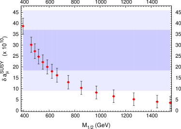
Figure 12: $\delta a_{\mu}^{\text{SUSY}}$ in the cNMSSM as a function of the unified gaugino mass $M_{1/2}$. The darker and brighter shaded areas show the 1–$\sigma$ respectively 2–$\sigma$ deviations from $\delta a_{\mu}=a^{\text{exp}}_{\mu}-a^{SM}_{\mu}$. Figure taken from (Djouadi:2008uj, ).

5.2.3 B-meson decay

The flavor changing neutral current decay $\Gamma(b\rightarrow s\gamma)$ is very sensitive to physics beyond the SM. The reason is, that this decay can only proceed via loops in the SM, thus is suppressed. Hypothetically postulated new particles may contribute to the decay. In supersymmetry there are lots of contributions, two examples are shown in Fig. 13, that is, a neutralino-sbino loop and a Higgs-boson–top loop.

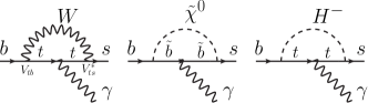
Figure 13: Example diagrams contributing to the $b\rightarrow s\gamma$ decay. The left diagram is a SM contribution, where also the CKM-matrix entries $V_{tb}$ and $V_{ts}^{*}$ are depicted. The mid- and right-diagrams show contributions occurring in supersymmetry via a neutralino–sbottom loop and a Higgs-boson–top loop, respectively.

However a quite good agreement of experimental observation and SM prediction of the $b\rightarrow s\gamma$ decay is found not allowing for a large additional total contribution. But, on the other hand, stringent constraints are put on every new model which postulates new particles which may contribute to this decay channel.

The experimental world average for the branching ratio (for a minimal photon energy of $E_{\text{min}}=1.6$ GeV) is presented by the Heavy Flavor Averaging Group (Barberio:2008fa, ) based on the measurements of BABAR (Aubert:2007my, ), Belle (Abe:2001hk, ) and CLEO (Chen:2001fja, ):

$$\operatorname{BR}^{\text{exp}}(b\rightarrow s\gamma)=(3.52\pm 0.25)\times 10^{-4}\,.$$ (87)

In contrast, the corresponding SM prediction (Gambino:2005dp, ) is, including the charm loop (Gambino:2001ew, ) as well as two-loop contributions (Adel:1993ah, ; Misiak:1994zw, ; Ali:1995bi, ; Pott:1995if, ; Greub:1996tg, ; Chetyrkin:1996vx, ; Greub:1997hf, ; Buras:1997xf, ; Kagan:1998ym, ; Gambino:2001ew, ; Buras:2002tp, ; Hiller:2004ii, )

$$\operatorname{BR}^{\text{SM}}(b\rightarrow s\gamma)=(3.73\pm 0.30)\times 10^{-4}\,.$$ (88)

That is, within the errors we have good agreement of the experimental data with the SM prediction. Thus, additional contributions from extensions of the SM are very restricted in case they contribute to the $b\rightarrow s\gamma$ decay.

5.3 Cosmological constraints

Supersymmetric extensions of the SM predict a stable lightest supersymmetric particle (LSP), as long as matter parity (or R-parity) is conserved. This LSP may account for the observed cold dark matter in the Universe. In the early Universe the LSP would be present in large numbers in thermal equilibrium. As the Universe has cooled the LSP’s only may reduce their density by pair annihilation and co-annihilation (Hut:1977zn, ; Vysotsky:1977pe, ; Lee:1977ua, ). As their density decreases, the chance to find another particle to annihilate decreases and at a certain point the comoving density can become constant (“freeze out”). The remaining relic density can be calculated depending on the considered model. In case the relic density of the LSP is identified with the cold dark matter candidate, a comparison with the cold dark matter observations constrain the model. We distinguish between direct detection of the relic density LSP particle in a detector and the indirect detection via astrophysical observations.

5.3.1 Indirect dark matter detection

The most stringent bound comes from the cosmic microwave background (CMB) observation performed by WMAP. The observed CMB is compared to the predictions of the standard model of cosmology, the so-called $\Lambda$-cold-dark-matter model ($\Lambda$CDM). This model depends on six parameters, the Hubble parameter $H_{0}$, the baryon density $\Omega_{b}h_{0}^{2}$, the cold dark matter density $\Omega_{c}h_{0}^{2}$, the dark energy density $\Omega_{\Lambda}$, the scalar spectral index $n_{s}$, the optical depth $\tau$, as well as the variation of the spectral index $n_{s}$ and the curvature perturbation $\Delta_{\cal R}^{2}$. By adjusting the parameters of the $\lambda$CDM, the prediction of the CMB power-spectrum can be fitted to the observation. Taking into account the recent five year WMAP data, combined with measurements of type Ia supernovae and baryon acoustic oscillations in the distribution of galaxies, the current 1–$\sigma$ limits on the $\Lambda$CDM parameters are given as (Hinshaw:2008kr, )

$$\begin{split}\Omega_{b}h_{0}^{2}&=0.02267^{+0.00058}_{-0.00059}\;,\\ \Omega_{c}h_{0}^{2}&=0.1131\pm 0.0034\;,\\ \Omega_{\Lambda}&=0.726\pm 0.015\;,\\ n_{s}&=0.960\pm 0.013\;,\\ \tau&=0.084\pm 0.016\;,\\ \Delta_{\cal R}^{2}&=(2.445\pm 0.096)\times 10^{-9}\text{ at }k=0.002~{}\text{Mpc}^{-1}\,,\end{split}$$ (89)

where we are in particular interested on the cold dark matter density $\Omega_{c}h_{0}^{2}$ constraint. Note that the Hubble constant is defined in terms of $h_{0}$, that is, $H_{0}=100\;h_{0}$ km/s/Mpc.

Now let us briefly sketch the calculation of the cold dark matter density in supersymmetric models. This relic density of the LSP as cold dark matter candidate, supposed to be a neutralino, can be computed by the solution of the continuity equation (Lee:1977ua, ; Vysotsky:1977pe, )

$$\frac{d}{dt}(n_{\tilde{\chi}}R^{3})=-\langle\sigma_{\text{ann}}v\rangle\left(n_{\tilde{\chi}}^{2}-(n_{\tilde{\chi}}^{\text{eq}})^{2}\right)R^{3}\,.$$ (90)

This continuity equation states that the number of neutralinos, with density $n_{\tilde{\chi}}$, in a comoving volume with radius $R$, is governed by the competition between annihilations and creations. The creations depend on the density of neutralinos in equilibrium $n_{\tilde{\chi}}^{\text{eq}}$. It is assumed that the annihilating particles have non-relativistic relative velocity $v$. Further, it is assumed that the annihilating particles as well as the annihilation products are maintained in kinetic equilibrium with the background thermal plasma through rapid scattering processes (Bernstein:1985th, ; Gondolo:1990dk, ). The model-dependent input is given by the thermally averaged annihilation cross section $\langle\sigma_{\text{ann}}v\rangle=a+bv^{2}$ with parameters $a$ and $b$. With this annihilation cross section the cosmic neutralino density can be deduced (Griest:1989zh, ; Kolb:1990vq, ; Drees:1992am, )

$$\Omega_{\tilde{\chi}^{0}}h_{0}^{2}=\frac{1.07\times 10^{9}\,x_{fr}}{\sqrt{g_{*}}M_{P}(a+\frac{3b}{x_{fr}})}\frac{1}{\text{GeV}}\;,$$ (91)

with $M_{P}$ the Planck mass and $g_{*}\approx 81$ the effective number of degrees of freedom at the freeze-out temperature $T_{fr}$ and $x_{fr}=m_{\tilde{\chi}}/T_{fr}$, where $m_{\tilde{\chi}}$ is the neutralino mass. In models like the MSSM and the NMSSM the annihilation cross section can be computed from s-channel Higgs and Z-boson exchange into fermions and gauge bosons, and from heavier neutralino or chargino t-channel exchange with gauge bosons in the final state. In particular for s-channel resonances, rapid annihilation can take place, reducing the relic density strongly. In the NMSSM, in contrast to the MSSM we have additional Higgs-boson resonances, contributing to the annihilation. In the case of light Higgs bosons in the NMSSM also new decay channels of neutralinos decaying into a $Z$ boson and a Higgs boson or two light Higgs bosons are available (Greene:1986th, ; Olive:1990aj, ; Abel:1992ts, ; Stephan:1997ds, ; Belanger:2005kh, ; Gunion:2005rw, ). Contrary, a large singlino component of the LSP reduces the annihilation cross section, since the singlino does not couple to gauge bosons at tree level.

In the investigation of Belanger et al. (Belanger:2005kh, ) the parameters of the NMSSM are scanned in particular with view on the dark matter constraint in (89). In this publication the program package micrOMEGAs (Belanger:2001fz, ) is employed, which, starting from the particle spectrum and couplings, computes the relevant annihilation and co-annihilation neutralino cross sections and eventually the relic density. The particle and coupling spectrum is provided by the NMHDECAY program (Ellwanger:2005dv, ). Assuming gaugino mass unification at the GUT scale ($M_{1/2}$), the independent parameters are $\lambda$, $\kappa$, $\tan(\beta)$, $\mu=\lambda v_{s}$, $A_{\lambda}$, $A_{\kappa}$. The authors find parameter space corresponding to a large singlino component of the neutralino LSP. This parameter space passes also the current collider constraints. Some representative examples are given in Tab. 3 (Belanger:2001fz, ).

parameters	1	2	3	4	5	6
$\lambda$	0.6	0.24	0.4	0.23	0.31	0.0348
$\kappa$	0.12	0.096	0.028	0.0037	0.006	0.0124
$\tan(\beta)$	2	5	3	3.1	2.7	5
$\lambda v_{s}$ [GeV]	265	200	180	215	210	285
$A_{\lambda}$ [GeV]	550	690	580	725	600	50
$A_{\kappa}$  [GeV]	-40	-10	-60	-24	-6	-150
$M_{2}$ [GeV]	1000	690	660	200	540	470
spectrum
$m_{\chi^{0}_{1}}$ [GeV]	122	148	35	10	15	203
$U_{13}^{2}+U_{14}^{2}$	0.12	0.29	0.12	0.03	0.06	0.02
$U_{15}^{2}$	0.88	0.69	0.87	0.95	0.94	0.96
$m_{\chi^{0}_{2}}$ [GeV]	259	199	169	87	182	214
$m_{\chi^{\pm}_{1}}$ [GeV]	258	193	171	139	196	266
$m_{H_{1}}$ [GeV]	117	116	36	22	34	115
$R_{13}^{2}$	0.88	0.04	0.98	1.00	1.00	0.04
$m_{H_{2}}$ [GeV]	128	158	117	114	113	163
$R_{23}^{2}$	0.11	0.96	0.01	0.00	0.00	0.96
$m_{A_{1}}$ [GeV]	114	59	56	18	15	214
$R_{45}^{2}$	0.99	1.00	0.99	1.00	0.99	1.00
dark matter study
$\Omega_{\tilde{\chi}^{0}}h_{0}^{2}$	0.1092	0.1179	0.1155	0.1068	0.1124	0.1023
channels	$HA$ (73%)	$VV$ (75%)	$qq$ (65%)	$qq$ (93%)	$AA$ (92%)	$\tilde{\chi}^{0}_{2}\tilde{\chi}^{0}_{2}\to X$ (81%)
	$VV$ (13%)	$HA$ (17%)	$ll$ (35%)	$ll$ (7%)	$qq$ (7%)	$\tilde{\chi}^{0}_{1}\tilde{\chi}^{0}_{2}\to X$ (15%)
	$ZH$ (8%)	$HH$ (5%)			$ll$ (1%)	$\tilde{\chi}^{0}_{1}\tilde{\chi}^{\pm}_{1}\to X$ (2%)
	$HH$ (3%)	$ZH$ (2%)				$qq$ (2%)
	$qq$ (2%)
	$ll$ (1%)

Table 3: Parameters with a LSP neutralino with a large singlino component ($U_{15}^{2}$) respecting the current collider as well as the cosmological dark matter constraints as presented in (Belanger:2005kh, ). The neutralino mass mixing matrix $U$ is defined in (161), the Higgs-boson mass mixing matrix $R$ is defined in (40). Here a CP-conserving Higgs sector is assumed.

In the upper part the initial NMSSM parameters are given, followed in the mid part by the particle spectrum and mixings and in the lower part by the dark matter study. Presented are the annihilation and co-annihilation channels which lead to the required relic density $\Omega_{\tilde{\chi}^{0}}h_{0}^{2}$ in the 3-$\sigma$ range of $\Omega_{c}h_{0}^{2}$; with view on (89). For the parameter points 3–5 there are very light LSP neutralinos which have, following from the neutralino mass mixing parameter $U_{15}^{2}$ (the matrix $U$ is defined in (161)), a large singlino component. In particular in these cases the dominating annihilation proceeds via Z- and Higgs-boson resonances. The parameter points 4 and 5 correspond to a light scalar Higgs boson which is dominantly a Higgs-boson singlet, as can be seen from the Higgs-boson mass mixing parameter $R_{13}^{2}\approx 1$ (the matrix $R$ is defined in (40)). In this case the lightest non-singlet SM-like Higgs boson has to pass the LEP bound. This in turn drives $\tan(\beta)$ close to 3, where the mass $m_{H_{2}}$ is maximized. In Fig. 14 the impact of the WMAP constraint on the parameter space is shown. The contours for different values of $\Omega_{\tilde{\chi}^{0}}h_{0}^{2}$ are given, where the black region corresponds to the WMAP constraint, that is, $0.0945<\Omega_{\tilde{\chi}^{0}}h_{0}^{2}<0.1287$. The chosen independent parameters are described in the figure caption. For further details see (Belanger:2005kh, ).

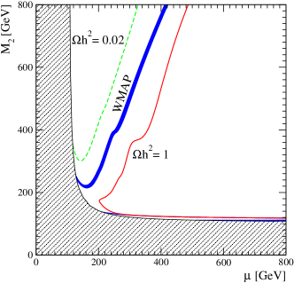
Figure 14: Contours for $\Omega_{\tilde{\chi}^{0}}h_{0}^{2}=0.02$, $0.0945$, $0.1287$, $1$ in the $\mu$–$M_{2}$ plane, as presented by (Belanger:2005kh, ). The remaining parameters are fixed to $\lambda=0.1$, $\kappa=0.1$, $\tan(\beta)=5$, $A_{\lambda}=500$ GeV, $A_{\kappa}=0$. The gaugino masses are assumed to unify at the GUT scale, corresponding at the electroweak scale to $M_{2}=2M_{1}$ and $M_{\tilde{g}}=3.3M_{2}$. The hatched region is parameter space which is excluded by LEP due to searches for chargino pairs (79); see (Belanger:2005kh, ) for further details.

The PAMELA satellite experiment finds an excess of positrons in cosmic rays Adriani:2008zr , whereas there is no excess of anti–protons found Adriani:2008zq . This could be explained in the NMSSM in a rather specific scenario Bai:2009ka . In this scenario the dark matter neutralinos can annihilate into the heavier pseudoscalar $A_{2}$ which subsequently decays into the lightest pseudoscalar $A_{1}$ and the CP-even $H_{1}$. In order to get a large annihilation cross section a resonant s-channel decay is assumed, forcing to have $m_{A_{2}}\approx 2m_{\tilde{\chi}^{0}}$. Further the neutralinos have to be lighter than the top quark to avoid a decay into a pair of top quarks which would yield an anti–proton access, which is not observed. For the same reason it is assumed that $m_{A_{1}}<1$ GeV such that the lightest pseudoscalar $A_{1}$ mainly decays into muons giving the observed positron excess and suppressing the decay of $A_{1}$ into mesons. In a parameter scan employing NMHDECAY (see App. B) parameter space is found which could explain both PAMELA observations with no contradiction to other constraints.

5.3.2 Direct dark matter detection

If the dark matter consists of unidentified particles, the earth should be passing through a flux of these particles which constitute the dark halo of our Milky Way. Direct detection of dark matter may then proceed via elastic scattering from a target nucleus. The nuclear recoil could then be detected in an appropriate detector. The corresponding event rate depends on the dark matter density in the solar vicinity and the model-dependent neutralino–nucleus elastic scattering cross section, under the assumption that neutralinos make up dark matter. For a fixed dark matter density (which is, following cosmological arguments about $\rho_{\text{DM}}\approx 300$ MeV/cm³) the flux of dark matter particles through a detector is obviously inverse proportional to its masses.
For investigations of direct neutralino dark matter detection in context with the NMSSM we mention the approaches (Flores:1991rx, ; Bednyakov:1998is, ; Cerdeno:2004xw, ; Gunion:2005rw, ; Cerdeno:2007sn, ). On the experimental side we draw the attention to the experiments of the DAMA collaboration (Bernabei:2008yi, ), CDMS (Ahmed:2008eu, ), EDELWEISS (Lubashevskiy:2008zz, ), ZEPLIN I (Alner:2005wq, ), as well as the XENON10 experiment (Angle:2007uj, ). Up to now there are no confirmed detections of any weakly interacting massive particle (WIMP). The sensitivities of some direct detection experiments are shown in Fig. 15 depending on the mass of the neutralino (Cerdeno:2007sn, ). The dots give predictions of the NMSSM varied in certain parameter ranges, as indicated in the figure caption. These points pass the LEP/TEVATRON, muon anomalous magnetic moment, and $BR(b\rightarrow s\gamma)$ constraints as discussed above in this section. The grey dots have passed the relic density constraint $0.1<\Omega_{\tilde{\chi}^{0}}h_{0}^{2}<0.3$ and the black dots even the much stronger constraint from the three-year WMAP data $0.095<\Omega_{\tilde{\chi}^{0}}h_{0}^{2}<0.112$. Obviously there is parameter space left which passes all the experimental and indirect/direct cosmological constrains in the NMSSM. As indicated in the figure, future direct dark matter detection experiments may give strong constraints of viable parameter space.

Figure 15: Scatter plot of the neutralino–nucleon cross section as a function of the neutralino mass, here denoted by $m_{\chi}$ for $\tan(\beta)=5$, and the remaining parameters varied in the ranges $0.01\leq\lambda$, $\kappa\leq 0.7$, $110~{}\text{GeV}<M_{2}<430~{}\text{GeV}$, $-300~{}\text{GeV}<A_{\kappa}<300~{}\text{GeV}$, $-800~{}\text{GeV}<A_{\lambda}<800~{}\text{GeV}$, $110~{}\text{GeV}<v_{s}\lambda<300~{}\text{GeV}$. All points pass the LEP/TEVATRON collider, muon anomalous magnetic moment, and $BR(b\rightarrow s\gamma)$ constraints and have a relic density in the range $0.1<\Omega_{c}h_{0}^{2}<0.3$ (grey dots) or $0.095<\Omega_{c}h_{0}^{2}<0.112$ (black dots) reflecting the three year WMAP data. The sensitivities of experiments are given by full lines, whereas the dashed lines give the sensitivities expected in the future. Figure taken from (Cerdeno:2007sn, ).

5.3.3 Baryogenesis

The absence of antimatter, that is, the observed baryon asymmetry in our Universe may be generated by strong electroweak phase transitions (EWPT) of first order (Kuzmin:1985mm, ; Shaposhnikov:1987tw, ; Rubakov:1996vz, ; Shaposhnikov:1996th, ). Alternatives to EWPT like GUT baryogenesis (Buchmuller:1996pa, ), baryogenesis via leptogenesis (Fukugita:1986hr, ) and the Affleck–Dine mechanism (Affleck:1984fy, ) are not discussed here. For an overview, see for instance (Riotto:1999yt, ). One of the attractive properties of EWPT is that this mechanism is understandable in terms of physics at the electroweak scale, accessible at current colliders. Our focus lies on the discussion of EWPT with respect to the NMSSM. We start with a brief sketch of EWPT and show how parameter constraints are deduced in the SM, the MSSM and in the NMSSM.

Phase transitions are generally characterized by an order parameter which suddenly changes at a critical temperature $T_{c}$. In case the order parameter has a discontinuity at $T_{c}$, the transition is called a first-order phase transition. In contrast, if the order parameter changes continuously at $T_{c}$, it is called a second-order phase transition. In the electroweak phase transition the order parameter is identified with the Higgs vacuum-expectation-value. Assuming a first order electroweak phase transition we have with decreasing temperature a transition from the symmetric phase with a global minimum at the origin for $T>T_{c}$ to a symmetry breaking phase with a global minimum with a vacuum-expectation-value at $v\neq 0$ for $T<T_{c}$. For $T=T_{c}$ we have degenerate minima at $v=0$ and $v=v_{c}$.

It has been shown that a strong first order phase transition is needed (Dine:1992vs, ; Dine:1992wr, ), that is

$$\frac{v_{c}}{T_{c}}>\xi\approx 1$$ (92)

in order to avoid a wash-out of the generated baryon asymmetry after it is generated.

Following closely the argumentation found in (Cline:2000fh, ; BasteroGil:2000bw, ) let us consider a generic Higgs potential

$$V_{\text{eff}}=m^{2}\phi^{2}-\alpha\phi^{3}+\beta\phi^{4}$$ (93)

with a generic scalar Higgs field $\phi$. From this potential we see that we get a first order phase transition, that is, degenerate minima with a symmetry breaking minimum at $v_{c}$, for

$$v_{c}=\frac{\alpha}{2\beta}.$$ (94)

Obviously we need a non-vanishing parameter $\alpha$, that is, a cubic term in the potential in order to get the wanted symmetry breaking minimum.

In the SM and in the MSSM we do not have a cubic term at all. Nevertheless, an effective cubic term is generated by thermal loops (Dolan:1973qd, ; Weinberg:1974hy, )

$$V_{\text{eff}}=V+V^{T}_{\text{1-loop}}$$ (95)

with

$$V^{T}_{\text{1-loop}}=T\sum_{i}\mp\int\frac{d^{3}p}{(2\pi)^{3}}\ln\bigg{(}1\pm e^{-\sqrt{p^{2}+m_{i}^{2}(\phi)/T}}\bigg{)}$$ (96)

with $i$ running over all fermions (upper sign) and bosons (lower sign), which couple to the Higgs boson. The expressions $m_{i}(\phi)$ are the corresponding field-dependent masses, that is, the masses depending on the Higgs field, before electroweak symmetry is broken. For high temperature $T$ the effective potential can be expanded as (Cline:2000fh, )

$$V^{T}_{\text{1-loop}}=\sum_{i}\frac{1}{48}m_{i}^{2}(\phi)\;T^{2}\cdot\left\{\begin{matrix}2\\ 4\end{matrix}\right\}-\frac{1}{12\pi}m_{i}^{3}(\phi)\;T\cdot\left\{\begin{matrix}1\\ 0\end{matrix}\right\}+\frac{1}{64\pi^{2}}m_{i}^{4}(\phi)\;\bigg{(}\ln\frac{m_{i}^{2}(\phi)}{T^{2}}-c_{i}\bigg{)}\cdot\left\{\begin{matrix}-1\\ 4\end{matrix}\right\}+{\cal O}\frac{m_{i}^{5}(\phi)}{T}\,,$$ (97)

where the upper line is valid for bosons and the lower one for fermions. The constants are

$$c_{i}=\begin{cases}\frac{3}{2}+2\ln(4\pi)-2\gamma_{E}\,,&{\text{for bosons}}\\ c_{\text{boson}}-2\ln(4)\,,&{\text{for fermions}}\end{cases}\,.$$ (98)

Obviously, we get for each boson in (97) an effective cubic term. For instance, for the field-dependent charged $W^{\pm}$-boson masses $m_{W^{\pm}}(\phi)=g_{2}\phi/\sqrt{2}$ a cubic $\alpha$-term in (93) is generated and first order phase transitions are possible.

In the SM however, these loop effects are too small, thus give only a too small $\alpha$-term. From the condition (92) one can deduce an upper bound on the Higgs-boson mass and gets (Cline:1998hy, )

$$m_{H}^{\text{SM}}<32~{}\text{GeV},$$ (99)

which is excluded from the lower bound on the Higgs-boson mass from the LEP experiment, $m_{H}^{\text{SM, exp}}>114$ GeV at 95% CL (Barate:2003sz, ). The conclusion is, that this mechanism of strong first order EWPT is not possible in the SM.

In the MSSM the situation is quite different. Let us sketch briefly the situation in this model. In Sect. 3.7 we have already seen that the tree-level mass of the lightest Higgs boson, $(m_{H_{1}}^{\text{MSSM}})^{2}<m_{Z}^{2}\cos^{2}(2\beta)$, is ruled out experimentally by LEP from the lower bound of $m_{H}^{\text{MSSM, exp}}>92$ GeV (Schael:2006cr, ). However, as we have discussed, there are quite large quantum corrections to this tree level mass. The largest contribution to the quantum corrections arise from top and stop loops, which couple strongly to the Higgs-bosons. We recall the one-loop radiative contribution to the lightest Higgs-boson mass (55),

$$(\Delta m_{H_{1}}^{\text{MSSM}})^{2}=c\frac{m_{t}^{4}}{v^{2}}\ln\left(\frac{m_{\tilde{t}_{L}}m_{\tilde{t}_{R}}}{m_{t}^{2}}\right)\,.$$ (100)

This correction allows for larger Higgs-boson masses passing the current LEP limits. From the logarithmic term we see that large radiative corrections require at least one of the masses $m_{\tilde{t}_{L}}$, $m_{\tilde{t}_{R}}$ to be very large. From precision electroweak constraints we know that $\tilde{t}_{L}$ has to be the heavy scalar. This follows from the fact that $\tilde{t}_{L}$ couples stronger to the electroweak gauge bosons than $\tilde{t}_{R}$ and a suppression of this loop contributions requires that $\tilde{t}_{L}$ is the heavier scalar. However, from the logarithmic dependence on $m_{\tilde{t}_{L}}$ of the mass shift (100) it follows that a substantial shift of the Higgs-boson mass requires a very large mass $m_{\tilde{t}_{L}}$.

Now we come to the thermic loops which potentially give a cubic term in (97) in the potential required for a strong first order EWPT (Carena:1996wj, ; Espinosa:1996qw, ; Bodeker:1996pc, ; Cline:1998hy, ). The field-dependent stop mass $m_{\tilde{t}_{R}}$ reads, taking also thermic corrections of the stop mass itself into account,

$$m_{\tilde{t}_{R}}^{2}=m_{\tilde{u}}^{2}+|y_{t}|^{2}|H_{u}^{0}|^{2}+c_{R}T^{2}\,,$$ (101)

with $c_{R}=4/9g_{3}^{2}+1/6|y_{t}|^{2}(1+\sin^{2}(\beta))$. A strong EWPT requires a large cubic term ($m_{i}^{3}(\phi)\sim\phi^{3}$ in (97)) and this in turn requires $m_{\tilde{u}}^{2}\approx-c_{R}T^{2}$. In the limit of zero temperature this means that we have to have a rather light $\tilde{t}_{R}$-mass. Altogether we find a mass hierarchy in the MSSM $m_{\tilde{t}_{R}}<m_{t}<<m_{\tilde{t}_{L}}$, which is considered to be unnatural, since it requires fine-tuning. In Fig. 16 the experimental 95% exclusion regions in the stop–neutralino mass plane are shown as presented by (Aaltonen:2007sw, ). We see that for a light neutralino, $m_{\tilde{\chi}}<45$ GeV, stop masses below 120 GeV are excluded. Thus, with respect to (100) we certainly need corrections of the order of 30 GeV in the MSSM, that is, rather large heavy scalar top mass $m_{\tilde{t}_{L}}$ compared to $m_{\tilde{t}_{R}}$, that is, large fine-tuning.

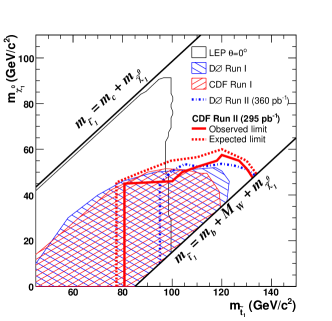
Figure 16: 95% exclusion regions in the stop–neutralino mass plane for the MSSM. Figure taken from (Aaltonen:2007sw, ).

In the NMSSM the strong electroweak phase transition requirement (92) is generically much easier fulfilled since already at tree level we have cubic terms in form of additional soft-breaking terms (Pietroni:1992in, ),

$$V_{\text{soft, trilinear}}=\lambda A_{\lambda}(H_{u}^{\mathrm{T}}\epsilon H_{d})S+\frac{\kappa}{3}A_{\kappa}S^{3}+c.c.$$ (102)

which are absent in the SM and the MSSM. Note that a cubic term in the generic Higgs potential can not be constructed in a gauge invariant way from Higgs doublets, since gauge invariance requires the Higgs doublets to occur in a bilinear or quartic form. Thus, an additional singlet Higgs field $S$, as introduced in the NMSSM, opens the possibility of cubic terms without relying on quantum corrections. Moreover, the tree-level mass limit on the lightest Higgs-boson mass in relaxed in the NMSSM.

There was some effort spent in systematical numerical parameter scans in order to find parameter space fulfilling the strong EWPT constraint (see for instance (Pietroni:1992in, ; Davies:1996qn, ; Huber:1998ck, ; BasteroGil:2000bw, )). Let us start with the study of Pietroni (Pietroni:1992in, ). The Coleman-Weinberg one-loop corrections (53) as well as the non-vanishing temperature contributions to the potential were taken into account (Dolan:1973qd, ; Weinberg:1974hy, ). The following assumptions were imposed.

• Common soft-breaking masses $m_{Q}^{2}=M_{1}^{2}=M_{2}^{2}\equiv 1$ TeV.

• Fixed values for $\lambda^{2}(m_{Z})=0.274$, $y_{t}(m_{Z})=0.97$ and $\kappa^{2}=1/2\lambda^{2}$.

• A minimal value for the singlet VEV $\lambda v_{s}\leq 45$ GeV, following approximatively from the experimental lower bound on the chargino mass.

• The ratio $\tan(\beta)$ is fixed to the values 2 and 10 and for the Higgs-boson mass parameters it is assumed that $m_{H_{d}}^{2}>0$, $m_{H_{u}}^{2}<0$ and $m_{S}^{2}>0$.

From a parameter scan it is found that the allowed parameter space leads to an upper bound of $m_{H}^{\text{NMSSM}}<170$ GeV for the lightest Higgs boson, far beyond the LEP limits.

In the work of Bastero-Gil et al. (BasteroGil:2000bw, ) also the parameter space is examined targeting on the requirement of strong first order EWPT. With different assumptions for the soft-breaking parameters as well as for the experimental LEP bounds it is shown that there is parameter space available in the NMSSM which also respects the LEP Higgs-boson mass bound.

Let us also mention the paper of Davies et al. (Davies:1996qn, ). The authors report that in a parameter scan passing appropriate constraints about one half of parameter points pass the strong first order EWPT condition. Under certain assumptions, not given here, they find masses of the lightest Higgs boson not exceeding 120 GeV. In this study also a generalization of the superpotential $W$ in (20) is introduced with an explicit $\mu$-term and a linear term:

$$W^{\prime}=W+\mu(H_{d}^{T}\epsilon H_{u})-rS\,.$$ (103)

Of course, by setting the dimensional parameters $\mu$ and $r$ to zero the original NMSSM is restored.

Eventually in the publication of Huber and Schmidt (Huber:1998ck, ) emphasis is placed on a subtle point in context with first order EWPT. As is pointed out, for an EWPT it is required, that phase transition in $v_{d}$, $v_{u}$ and $v_{s}$ have to occur simultaneously. This means that all three vacuum-expectation-values should be of the same order of magnitude. If one has for instance a much larger value $v_{s}$ compared to $v_{d}$ and $v_{u}$, a cascade of phase transitions would occur with decreasing temperature. This would not correspond to a first order phase transition which needs a bump in the effective potential, requiring a trilinear term in the Higgs fields. The authors refer to the parameter scans of Ellwanger et al. (see the discussion in Sect. 5.4), which predict a generic larger value for $v_{s}$ compared to the doublet VEVs. In order to circumvent this problem it is proposed that the supplemented superpotential (103) should be taken into account. In this way a compatible vacuum-expectation-value $v_{s}$ of the electroweak order arises. However, as is pointed out by the authors, the generic larger values of $v_{s}$ arise in studies, where the assumption of unification of soft-breaking parameters at the GUT scale or other additional constraints are considered. As we will see in the next subsection, dropping the unification condition meets the criterion of a VEV $v_{s}$ of the electroweak order also without a modification of the NMSSM superpotential.

5.4 Parameter scans

A quite generic approach in order to constrain the parameter space of a model is to scan over the parameter ranges of interest. For each parameter set in this scan the particle mass and coupling spectrum is derived. Then, the viability of this spectrum is checked, for instance with respect to the corresponding minimum structure: only a parameter set corresponding to a global minimum in the Higgs potential with the observed electroweak symmetry breaking is to be accepted in this scan. Moreover, the different experimental and cosmological constraints on the masses and couplings have to be passed. From the eventually gained allowed parameter space, which passes all constraints, restrictions can be read off. In this section we want to present only some of the various scans which have been performed in the NMSSM (Ellwanger:1991bq, ; Ellwanger:1995ru, ; Ellwanger:1996gw, ; Stephan:1997rv, ; Djouadi:2008uj, ). Typically, they are based on computer tools which calculate the spectrum and apply various theoretical and experimental constraints. Due to the large number of parameters in the NMSSM typically not the full parameter space is scanned over for practical reasons. This is in particular true for the rich part of parameters originating from the soft supersymmetry breaking terms. Note that in the discussion of Higgs-boson phenomenology in Sect. 3.7 already some studies based on parameter scans were mentioned. Assumptions like the unification of parameters at a high scale like the GUT scale lead to an enormous reduction of available parameter space and thus simplify the investigation. Therefore, most of the parameter scan studies are applied to the constrained NMSSM (cNMSSM); see App. E. We start with briefly discussion some of these studies in the cNMSSM followed by a parameter scan in the general NMSSM without unification assumption.

Let us first mention a series of investigations of the cNMSSM by Ellwanger et al. (Ellwanger:1991bq, ; Ellwanger:1995ru, ; Ellwanger:1996gw, ). For each of about one million points in the five-dimensional parameter space, the particle and coupling spectrum of the model at the electroweak scale is generated by the renormalization group equations. Then, the following constraints are applied:

• Large trilinear soft $A$-parameters may induce electrically charged or colored vacua; see (74). Since this is phenomenologically unacceptable, the corresponding parameter sets are discarded.

• The global minimum is searched for numerically and the global minimum is required to have non-vanishing Higgs VEVs $v_{d}$, $v_{u}$ and $v_{s}$. In this, the effective one-loop Higgs potential is considered, taking the Coleman–Weinberg contributions (53) into account. The ratio of the VEVs $v_{d}$ and $v_{u}$ is forced to comply with $\tan(\beta)<30$.

• The top-quark mass, as derived from the particle mass spectrum, is forced to fulfill the experimental constraints, that is, 168 GeV $<m_{t}<$ 192 GeV. Also it is checked that the negative search for charginos $m_{\tilde{\chi}^{\pm}}$ is not violated; see (79).

It is found that low values of the parameters $\lambda$ and $\kappa$ are favored as well as a large value of the singlet VEV $v_{s}$. This means that the singlet is decoupled and the NMSSM mimics the MSSM under the unification assumption. Nevertheless, there remains parameter space where one neutralino has a large singlino component and thus substantial differences may arise compared to the MSSM. It is pointed out (see for instance (Djouadi:2008uj, )) that for small parameters $\lambda$ and $\kappa$, the two parameters $m_{S}^{2}$ and $A_{\kappa}$ change not very much between the electroweak and the GUT scale by the renormalization group equations, that is, from (76) the unification parameter constraints $m_{0}^{2}\lesssim 1/9A_{0}^{2}$ is evident. Note that there is a subtle difference between the cMSSM and the cNMSSM: In the cMSSM small values of the $m_{0}$ parameter are disfavored since they lead to a charged slepton LSP, unacceptable as a dark matter candidate. Contrary, in the cNMSSM a small parameter $m_{0}$ is favored due to a viable global minimum for non-vanishing $v_{s}$. The slepton LSP in the cNMSSM is avoided since the possibility of a singlino-like LSP arises in parameter space (Hugonie:2007vd, ).

We would also like to mention the approach of Stephan (Stephan:1997rv, ). This study is also performed in the constrained NMSSM. The main difference to the previously discussed approaches is that in this work in addition the dark matter constraint, that is, the relic abundance of the LSP, supposed to be a neutralino, is taken into account. There are also some subtle points concerning some deviating theoretical and experimental constraints, which are applied. Starting with $5.5\cdot 10^{8}$ points in the five-dimensional parameter space, about 4900 points pass the theoretical and experimental constraints but only 2000 points of these pass the cosmological constraint given by the relic neutralino abundance bound. Quite restrict explicit bounds are derived in this way and given already in the abstract of this work:

$$m_{H_{1}}<140\text{ GeV}\,,$$

$$m_{\tilde{\chi}^{0}}<300\text{ GeV}\,,$$

$$m_{\tilde{e}_{R}}<300\text{ GeV}\,,$$

$$300\text{ GeV}~{}<m_{\tilde{u}_{R}}<1900\text{ GeV}\,,$$

$$200\text{ GeV}~{}<m_{\tilde{t}_{1}}<1500\text{ GeV}\,,$$

$$350\text{ GeV}~{}<m_{\tilde{g}}<2100\text{ GeV}\,.$$

Scatter plots in the $m_{\tilde{e}_{R}}$–$m_{\tilde{\chi}_{1}^{0}}$ plane are shown in Fig. 17 for the cMSSM as well as for the cNMSSM. Note that in the cNMSSM the selectron mass $m_{\tilde{e}_{R}}$ is stronger constrained than in the cMSSM. As mentioned above this arises from favored lower values of $m_{0}$, whereas in the cMSSM small values of $m_{0}$ are disfavored. An upper bound of $m_{0}\approx m_{\tilde{e}_{R}}$ can be deduced based on the relic density constraint which requires to have nearly degenerate masses of the LSP and the NLSP (Djouadi:2008uj, ). From an approximation for the RGE running of the NLSP mass it is found that $m_{0}^{2}\lesssim 1/15M_{1/2}^{2}$, favoring low values of $m_{0}\approx m_{\tilde{e}_{R}}$ in the cNMSSM in contrast to the cMSSM. Also the strong effect of the application of the relic abundance dark matter constraint is demonstrated in this figure.

Figure 17: Scatter plots in the constraint cMSSM (upper part) compared to the constrained cNMSSM (lower part) in the $m_{\tilde{e}_{R}}$–$m_{\tilde{\chi}_{1}^{0}}$ plane. The right part shows the scatter plots passing also the WMAP dark matter (denoted by d.m.) constraint. Figure taken from (Stephan:1997rv, ).

In the work of Bastero-Gil et al. (BasteroGil:2000bw, ), the MSSM is compared to the NMSSM. In this study emphasis is placed on the fine-tuning required in both models in order to comply with the theoretical and experimental constraints. Fine-tuning is quantified quite similar to (71), in the form

$$\Delta^{\text{max}}=\mathop{\max}_{a_{i}}\left|\frac{a_{i}}{m_{Z}^{2}}\frac{\operatorname{d}m_{Z}^{2}}{\operatorname{d}a_{i}}\right|\;,$$ (104)

where $a_{i}$ denotes all the soft supersymmetry breaking parameters. In a parameter scan the unified scalar mass is fixed, $m_{0}=100$ GeV, as well as the $A$-parameters, $A_{\kappa}(m_{Z})=0$, $A_{t}(\Lambda_{G})=0$ and the gaugino masses $M_{1}(\Lambda_{G})=M_{2}(\Lambda_{G})=500$ GeV, where $\Lambda_{G}$ denotes the GUT scale. The gaugino mass $M_{\tilde{g}}$ is varied in the range 100 GeV $<M_{\tilde{g}}(\Lambda_{G})<600$ GeV, and the Higgs-boson mass parameter $m_{H_{d}}$ is devoted to $0<m_{H_{d}}(\Lambda_{G})<1$ TeV, with $\mu=\lambda v_{s}<0$. In the NMSSM also the additional parameters $\lambda(\Lambda_{G})=1$ and $\kappa(\Lambda_{G})=0.1$ are fixed. Requiring further for the chargino masses $m_{\tilde{\chi}^{\pm}}>90$ GeV, the values for the fine-tuning function $\Delta^{\text{max}}$ are given in Fig. 18 for $\tan(\beta)=3$ and $\tan(\beta)=5$, respectively.

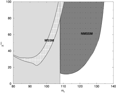
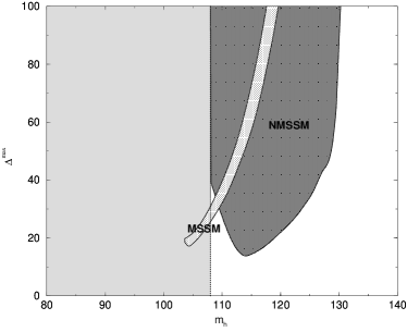
Figure 18: Scatter plot of fine-tuning as defined in (104) as a function of the lightest physical Higgs-boson mass for $\tan(\beta)=3$, left, and $\tan(\beta)=5$, right. In this scan there are fixed values of $m_{0}=100$ GeV, $A_{t}(\Lambda_{G})=0$, $M_{1}(\Lambda_{G})=M_{2}(\Lambda_{G})=500$ GeV, $\mu=\lambda v_{s}<0$ and varied parameters $M_{\tilde{g}}(\Lambda_{G})$, $m_{H_{d}}(\Lambda_{G})$ and $m_{H_{u}}(\Lambda_{G})$. The dark shaded regions shows the fine-tuning values corresponding to the NMSSM and the brighter shaded regions corresponding to the MSSM. The LEP limit on the SM Higgs-boson with $m_{H}^{\text{SM}}<108$ mass is also shaded. Figure taken from (BasteroGil:2000bw, ).

Let us cite the authors: The plots are a striking demonstration that the physical Higgs boson can be heavier and involve less fine-tuning in the NMSSM compared to the MSSM at low values of $\tan\beta$. The large fine-tuning in the MSSM for low $\tan(\beta)$ originates from the LEP bounds on the minimal Higgs-boson mass confronting the tree-level prediction of a mass below the $Z$-boson mass $m_{Z}$. Thus, large quantum corrections to the Higgs-boson mass in turn require a very large stop mass, that is, large fine-tuning. On the other hand it is pointed out that low values of $\tan(\beta)$ are favored in order to have a strong electroweak phase transition. The authors conclude that in the NMSSM the situation is much better with respect to the LEP bound on the minimal Higgs-boson mass, fine-tuning and baryogenesis via first order EWPT.

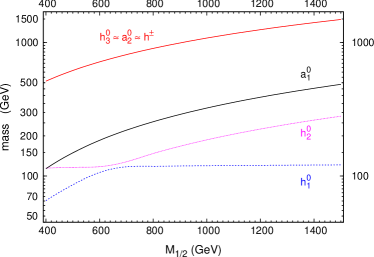
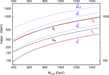
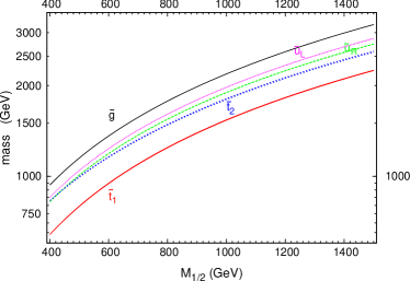
Figure 19: Spectrum of Higgs bosons in the upper plot (here denoted with small letters), neutralino-, selectron- and stau-mass spectrum in the left plot and squark- and gluino-mass spectrum in the right plot. The unified scalar mass is set to $m_{0}=0$. Degeneracy of the masses $m_{\tilde{\chi}^{\pm}_{1}}=m_{\tilde{\chi}_{3}}$ and $m_{\tilde{\chi}^{\pm}_{2}}=m_{\tilde{\chi}_{4/5}}$ is found. Plots taken from (Djouadi:2008uj, ).

In a recent study by Djouadi, Ellwanger and Teixeira (Djouadi:2008uj, ), focusing also on the cNMSSM, very severe constraints are found. After applying the theoretical as well as current experimental constraints, including the new WMAP data on the relic density, there remains a quite narrow window of allowed parameter space. It is reported that in the cNMSSM, the gluino $\tilde{g}$ turns out to be generically heavier than all squarks $\tilde{q}$. The NLSP is found to be generically stau-like and nearly degenerate with the LSP mass which is a neutralino, reflecting the constraints coming from the relic density. The supersymmetric partner particles eventually decay via the stau-like NLSP into the LSP neutralino. This opens the possibility of the observation of displaced vertices as discussed in Sect. 4. The particle spectra of the neutralinos, charginos, selectron and stau as well as the spectra of squarks and gluino are shown in Fig. 19. In this figures, the unified scalar mass is fixed to zero, $m_{0}=0$ (also another choice of the unified scalar mass is discussed in the paper). We see that the spectra of supersymmetric partner particles are highly restricted by the theoretical and experimental bounds, where also the current WMAP constraint for the relic density is applied; see (89). As the authors of this investigation have stressed, the measurement of one sparticle mass or mass difference would allow to predict quite accurately the complete sparticle spectrum in the cNMSSM.

Let us also mention the approach of Bednyakov and Klapdor-Kleingrothaus (Bednyakov:1998is, ), targeting mainly at the direct detection of a LSP neutralino dark matter candidate. This direct detection refers to elastic scattering of a dark matter neutralino from a nucleus producing a nuclear recoil detected in an appropriate detector; see Sect. 5.3. In this work no unification at the GUT scale of soft parameters is assumed, that is, there is no need to apply the RGE’s from the GUT scale starting point in this case. The scan is done over the eleven-dimensional parameter space

$$M_{1},M_{2},\tan(\beta),v_{s},\lambda,\kappa,m_{Q_{1}},m_{Q_{3}},A_{u_{3}},A_{\lambda},A_{\kappa},$$ (105)

with $m_{Q_{1}}=m_{Q_{2}}$, $m_{Q_{3}}$ the soft mass parameters with generation index. For simplicity reasons it is assumed that $m_{Q_{2}}^{2}\equiv m_{\tilde{u}_{1,2}}^{2}=m_{\tilde{d}_{1,2}}^{2}=m_{L_{1,2}}^{2}=m_{\tilde{e}_{1,2}}^{2}$ and $m_{Q_{3}}^{2}\equiv m_{\tilde{u}_{3}}=m_{\tilde{d}_{3}}=m_{L_{3}}=m_{\tilde{e}_{3}}$. Moreover it is set $A_{u}=A_{d}=A_{e}\equiv 0$ for all generations except $A_{u_{3}}$. The soft supersymmetry breaking parameters are defined in (150). Negative results for the search for supersymmetric particles at LEP and at TEVATRON are included in the analysis. The resulting allowed parameter space is compared once without any cosmological constraint on the co-annihilation rate of the LSP and once taken the constraint $0.025<\Omega_{\tilde{\chi}^{0}}h_{0}^{2}<1$ into account. This cosmological constraint alone gives, as is reported, a 20% cut on the allowed parameter space. As is pointed out in their conclusion, under their assumptions, but without unification of soft supersymmetry breaking parameters at the GUT scale, there remain domains in parameter space where the lightest neutralino has a quite small mass, even as small as 3 GeV. In this work it is stressed that in a proposed germanium ${}^{73}Ge$ detector there are large event rates expected in the NMSSM. Let us remark, that with view on the current WMAP data, it would be very interesting to see the effect of the current much tighter bounds in this study; see (89).

Finally, it is clear that the results of the here discussed parameter scans depend strongly on the assumptions taken into account, like the unification of parameters. On the other hand are the results also strongly dependent on the constraints applied to the derived particle and coupling spectra. To summarize, we have seen that at least for the general NMSSM, without any unification assumptions, there is a lot of viable parameter space, even if the cosmological LSP cold dark matter constraint is taken into account. Nevertheless, even that the cNMSSM seems to be very restricted, it remains a viable model with respect to all applied theoretical and experimental bounds.

6 Determining the global minimum of the Higgs potential

It is a non-trivial task to find the global minimum of Higgs potentials with a large number of Higgs-boson fields. For instance in the NMSSM the Higgs-boson sector consists of two complex electroweak doublets and one complex electroweak singlet, that is, 8 real fields from the doublets plus 2 real fields from the singlet. The conventional approach based on the unitary gauge requires the global minimum to be found in a 7-dimensional field space. Typically, numerically methods are applied in such involved cases in order to determine the global minimum; in contrast, here we want to discuss an algebraic approach (Maniatis:2006jd, ). In this approach all stationary points of the tree-level Higgs potential are found and supposed, the potential is bounded from below, the global minimum is identified from the corresponding lowest value of the potential. The method is applied to the NMSSM, revealing a quite surprising structure of stationary points, that is minima, maxima, and saddle points with different behavior with respect to the symmetry breaking of the $SU(2)_{L}\times U(1)_{Y}$ electroweak gauge group.

The global minimum of the Higgs potential gives the expectation values of the Higgs fields at the stable vacuum. Parameter values for the Higgs potential are thus considered to be acceptable only, if the global minimum of the Higgs potential occurs for Higgs-field vacuum-expectation-values, which induce the spontaneous breakdown of $SU(2)_{L}\times U(1)_{Y}$ to the electromagnetic $U(1)_{em}$ at the electroweak scale $v\approx 246$ GeV.

Firstly, the tree level Higgs potential for general models with two Higgs doublets and an arbitrary number of additional Higgs singlets is considered. The first step is to recognize that the potential is restricted by renormalizability and gauge invariance. Renormalizability restricts the potential to at most quartic terms in the Higgs fields. Electroweak gauge invariance restricts the possible doublet terms in the potential, since only gauge invariant scalar products of doublets can occur. Substituting the doublet fields by appropriate functions of these invariant scalar products, all gauge degrees of freedom can be eliminated. The method to base the analysis on bilinear gauge-invariant functions was introduced already in context with the general two-Higgs doublet model (Nagel:2004sw, ; Maniatis:2006fs, ).

The global minimum is among the stationary points of the potential. The stationarity conditions of the Higgs potential form non-linear, multivariate, inhomogeneous polynomial systems of equations of third order. A systematic approach to solve these – in general quite involved – systems of polynomial equations is possible by a Groebner basis computation, well established in ideal theory (Buchberger, ; Bose, ; Weispfenning, ). The Groebner basis was originally introduced to solve the ideal membership problem. Constructing this Groebner basis with an appropriate ordering of the monomials (see App. H for an illustration of the Groebner basis approach and further details), for instance the lexicographical ordering, and subsequent triangularization allows to solve the initial system of equations algorithmically for any finite number of complex solutions. The introduction of gauge invariant functions just avoids continuous gauge symmetries in the potential and the finiteness of the set of complex solutions can be easily checked within this algorithmic approach. Moreover, this approach guarantees that all stationary points are found.

In Maniatis:2006jd the method is applied to the NMSSM. For the computation of Groebner bases as well as the subsequent steps to solve the systems of equations the freely available open-source algebra program SINGULAR (Singular, ) is employed. It is found that large parts of the parameter space of the NMSSM Higgs potential can be excluded by requiring the global minimum to have the electroweak symmetry breaking observed in Nature. This is illustrated by determining the allowed and forbidden ranges for some generic parameters of the model.

6.1 Stationary points in the NMSSM

The NMSSM Higgs potential is given in Sect. 3.1 with parameters

$$\lambda,\kappa,m_{H_{u}}^{2},m_{H_{d}}^{2},m_{S}^{2},A_{\lambda},A_{\kappa}.$$ (106)

The quartic terms of the potential (26) are positive for any non-trivial field configuration, if both $\lambda$ and $\kappa$ are non-vanishing. The potential is therefore bounded from below for all cases considered here, and stability needs not to be checked any further.

The NMSSM Higgs potential is translated to the formalism described in App. G, where all Higgs-doublet scalar products are replaced by real gauge-invariant functions, $K_{0}$, $K_{1}$, $K_{2}$, $K_{3}$ and the complex singlet field is decomposed into two real fields according to $S=S_{re}+iS_{im}$. In this notation the Higgs potential $V=V_{\text{F}}+V_{\text{D}}+V_{\text{soft}}$ is given by

$$\begin{split}V_{\text{F}}=&\;\frac{1}{4}|\lambda|^{2}\left(K^{2}_{1}+K^{2}_{2}+4K_{0}(S^{2}_{re}+S^{2}_{im})\right)\\ &+|\kappa|^{2}(S^{2}_{re}+S^{2}_{im})^{2}\\ &-\operatorname{Re}(\lambda\kappa^{*})\left(K_{1}(S_{re}^{2}-S_{im}^{2})+2K_{2}S_{re}S_{im}\right)\\ &+\operatorname{Im}(\lambda\kappa^{*})\left(K_{2}(S^{2}_{re}-S^{2}_{im})-2K_{1}S_{re}S_{im}\right),\\ V_{\text{D}}=&\;\frac{1}{8}(g_{1}^{2}+g_{2}^{2})K_{3}^{2}+\frac{1}{8}g_{2}^{2}\;\left(K^{2}_{0}-K^{2}_{1}-K^{2}_{2}-K^{2}_{3}\right),\\ V_{\text{soft}}=&\;\frac{1}{2}m_{H_{u}}^{2}\;(K_{0}-K_{3})+\frac{1}{2}m_{H_{d}}^{2}\;(K_{0}+K_{3})\\ &+m_{S}^{2}\;(S^{2}_{re}+S^{2}_{im})\\ &-\operatorname{Re}(\lambda A_{\lambda})\left(K_{1}S_{re}-K_{2}S_{im}\right)\\ &+\operatorname{Im}(\lambda A_{\lambda})\left(K_{2}S_{re}+K_{1}S_{im}\right)\\ &+\frac{2}{3}\operatorname{Re}(\kappa A_{\kappa})\left(S_{re}^{3}-3S_{re}S_{im}^{2}\right)\\ &+\frac{2}{3}\operatorname{Im}(\kappa A_{\kappa})\left(S_{im}^{3}-3S_{re}^{2}S_{im}\right).\end{split}$$ (107)

For given values of the potential parameters (106) all stationary points of the NMSSM can be found by solving the systems of equations (214), (216), (218) as described in App. G.

The initial parameters in the Higgs potential (106) are translated to the set of parameters as described in Sect. 3.5. This enables for instance to fix the vacuum expectation values $v$, $\tan(\beta)$ and $v_{s}$. As a numerical example the parameter are chosen as

$$\begin{gathered}\lambda=0.4,\quad\kappa=0.3,\quad\left\lvert{A_{\kappa}}\right\rvert=200\text{~{}GeV},\\ \tan\beta=3,\quad m_{H^{\pm}}=2v,\\ \operatorname{sign}{R_{\kappa}}=-,\quad\delta_{\text{EDM}}=0,\quad\delta_{\kappa}^{\prime}=0\end{gathered}$$ (108)

and the parameter $v_{s}$ is varied. The roots of the univariate polynomials are found numerically, with a precision of $100$ digits. The approach allows to use arbitrary precision. The errors of the approximate statements described in the following are checked to be under control. For generic values of the parameters $52$ complex solutions are found: $7$ corresponding to the unbroken, $38$ to the partially broken, and $7$ to the fully broken cases. The number of real and therefore relevant solutions depends on the specific values of the parameters.

As expected from the $\mathbbm{Z}_{3}$ symmetry of the potential, either 1 or 3 solutions sharing the same value of the potential are found within the accuracy of the numerical roots. From the computed stationary points only those may be accepted as global minima which correspond to the initial vacuum expectation values (up to the complex phases), that is, which fulfill

$$\sqrt{2K_{0}}\approx v,\;\;\sqrt{\frac{K_{0}-K_{3}}{K_{0}+K_{3}}}\approx\tan\beta,\;\;\sqrt{2({S_{re}^{2}+S_{im}^{2}})}\approx v_{s}.$$ (109)

Since for non-vanishing parameters $\lambda,\kappa$ the potential is bounded from below, the stationary point with the lowest value of the potential is the global minimum.

In Fig. 20 the values of the potential at all stationary points for the parameter values (108) with varied $v_{s}$ is shown (Maniatis:2006jd, ).

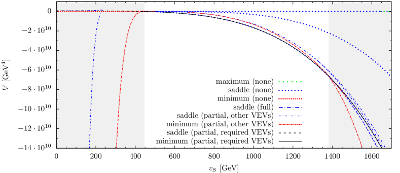
Figure 20: Values of the NMSSM Higgs potential at its stationary points in dependence on $v_{s}$, as presented in (Maniatis:2006jd, ). The parameters of the Higgs potential are chosen as $\lambda=0.4,\kappa=0.3,\left\lvert{A_{\kappa}}\right\rvert=200\text{ GeV},\tan(\beta)=3,m_{H^{\pm}}=2v,\operatorname{sign}{R_{\kappa}}=-,\delta_{\text{EDM}}=\delta_{\kappa}^{\prime}=0$. Each line corresponds to 1 or 3 stationary points sharing the same value of the potential. The different line styles denote saddle points, maxima, and minima. The labels ’none’, ’full’, and ’partial’ denote solutions of the classes with unbroken (214), fully broken (216), and partially broken (218) $SU(2)_{L}\times U(1)_{Y}$, respectively. For solutions of the partially broken class, it is also denoted whether they correspond to the ’required VEVs’ $v_{u},v_{d},v_{s}$ or to ’other VEVs’. Excluded parameter values, where the global minimum does not exhibit the required vacuum expectation values, are shown by shaded area.

Each curve in the figure represents 1- or 3-fold degenerate stationary potential values, where the gauge symmetry breaking behavior of the solutions is denoted by different line styles. Excluded parameter regions, where the global minimum does not exhibit the required expectation values (109) are shown shaded. As is illustrated in the figure, substantial regions of the NMSSM parameter space are excluded. For some excluded parameter regions, the partially breaking solutions with the required vacuum expectation values (109) are saddle points. This means they can be discarded as global minima without calculation of the other stationary points. However, this is not always the case. Obviously from Fig. 20, an upper bound for $v_{s}$ is found. For the plotted $v_{s}$ larger than this upper exclusion bound the solutions fulfilling (109) are still pronounced minima, i.e. the mass matrices have positive eigenvalues, but they are no longer the global minima. Also there are non-breaking saddle points with potential values slightly above those of the wanted global minimum. It is found that this effect is not coincidental for the initial parameters (108) chosen, but rather a generic feature of the NMSSM. Within the CP conserving parameter range

$$\begin{gathered}\lambda\in\,]0,1],\quad\kappa\in\,]0,1],\quad A_{\kappa}\in\pm\,]0,2500]\text{ GeV},\\ \tan\beta\in\,]0,50],\quad v_{s}\in\,]0,5000]\text{ GeV},\\ m_{H^{\pm}}\in\,]0,2500]\text{ GeV}\end{gathered}$$ (110)

samples are selected, producing the wanted global minimum and typically non-breaking saddle points are found, where the relative separation of the potential values for the saddle points and the global minimum is below the per-mill level, in many cases even far below. No fully breaking global minima are found for scenarios in the range (110) where the solutions with the required vacuum expectation values (109) are local minima. Eventually, there are examples, where CP conserving parameters with the “wrong” global minimum produce the wanted global minimum if a non-vanishing phase $\delta_{\kappa}^{\prime}$ is introduced.

7 Summary

The MSSM suffers from the $\mu$-problem, that is, the dimensionful $\mu$-parameter has to be adjusted by hand to the electroweak scale. In the NMSSM an effective $\mu$-term is generated dynamically. To this purpose an extra singlet superfield is introduced. Via spontaneous symmetry breaking the Higgs-boson singlet acquires a vacuum-expectation-value and generates the required $\mu$-term dynamically.

However, as we have seen, absence of the $\mu$-term in the superpotential imposes a continuous symmetry, the Peccei–Quinn-symmetry. An additional cubic self-coupling term of the singlet is introduced in order to break the Peccei–Quinn-symmetry which would lead to an unobserved axion. That is, the PQ-symmetry is promoted to a $\mathbbm{Z}_{3}$-symmetry, which, since spontaneously broken, leads to the formation of dangerous domain walls. The loophole is to impose higher order operators and additional symmetries, breaking the $\mathbbm{Z}_{3}$-symmetry but not disturbing physics at the electroweak scale.

In the NMSSM we encounter two more Higgs bosons as well as a fifth neutralino; compared to the MSSM. The modified mixing matrices were recalled in the Higgs sector as well as in the neutralino sector. Also the physical potential was derived, yielding, in particular, additional trilinear $A$-parameter terms.

The theoretical and experimental constraints on the model were discussed. On the theoretical side restrictions arise from the symmetries of the physical potential. Thus a global minimum which is electric- or color-charge breaking is forbidden, as well as a minimum with the wrong electroweak symmetry breaking behavior. Stability of the potential is of no concern, since for a non-vanishing Peccei–Quinn-symmetry breaking $\kappa$-parameter quartic terms in the potential ensure a potential which is bounded from below.

Further theoretical constraints come from the requirement of perturbativity of the couplings up to the GUT or Planck scale. Of course, this condition relies on the viability of the model up to large scales. In a series of recent publications the argument of fine-tuning got a lot of attention. On a quantitative basis, studies of fine-tuning in different scenarios in the NMSSM as well as compared to the MSSM were performed, revealing that in general there is much less fine-tuning in the NMSSM. This fine-tuning arises mainly from the stop-loops entering logarithmically in the Higgs-boson selfenergy. In particular, the LEP bounds require to have large radiative corrections accompanied by very large stop masses in the MSSM. Compared to the MSSM, the Higgs sector is much less constraint, that is, the NMSSM passes the LEP constraints with much less fine-tuning.

We proceeded with a discussion of the experimental constraints. First of all the electroweak precision measurements were discussed, which agree well with the SM predictions. Especially the invisible $Z$-boson decay puts severe constraints on the NMSSM, but also the constraint of limits on neutralino/chargino- and charged Higgs-boson pair production at LEP was discussed.

The impact of the muon anomalous magnetic moment, measured at BNL, on the NMSSM was presented. From chargino–sneutrino and neutralino–smuon loops we get additional contributions to the anomalous magnetic moment compared to the SM. Based on accurate SM predictions, which are not yet available, strong constraints on the parameter space in the NMSSM could be derived.

Also the $b\rightarrow s\gamma$ decay was considered, which, since loop-induced, is very sensitive to new particles, which couple to SM particles. Here the measurement agrees well with the SM prediction, yielding an additional constraint for new contributions which arise in extensions of the SM. Also in this respect the NMSSM does not violate this constraint significantly in large parts of parameter space.

The new five-year WMAP data give accurate predictions of cold dark matter in the Universe based on the $\Lambda$CDM. Since supersymmetric models, respecting matter-parity, predict a new stable particle, they provide a natural cold dark matter candidate, the LSP. The WMAP constraint on the LSP turns out to be very strong in the NMSSM and restricts the available parameter space enormously. Likewise, in the constraint NMSSM, where unification of the scalar mass, of the gaugino mass, and of the trilinear $A$-parameter at the GUT scale is assumed, the theoretical and experimental constraints are shown to be highly restrictive.

Strong first order electroweak phase transitions in order to account for the observed baryon–antibaryon asymmetry in our Universe require a cubic term in the physical potential. With this respect the SM as well as the MSSM rely on loop contributions in the effective potential which are generically small. In contrast, in the NMSSM, the additional trilinear terms allow to accomplish for this mechanism of baryogenesis without large fine-tuning.

Some recent parameter scans were reviewed with quite interesting results, constraining the NMSSM parameter space. Some emphasis was placed on a “no-lose”-theorem, that is, the question whether at least one Higgs-boson is detectable at the LHC with high integrated luminosity. The Higgs-to-Higgs decays are found to be rather difficult to detect, which however correspond to large parameter space. New ideas to detect such signatures were reviewed. However there seems to be some parameter space left, where all supersymmetric partner particles could escape detection. An electron–positron collider could close this gap in detecting the recoil mass in signatures of Higgs-boson production in invisible $Z$-strahlung. Some publications were reviewed discussing how to distinguish the NMSSM from the MSSM. The fifth neutralino may lead to a very different signature in colliders. In case the LSP is a singlino-like neutralino, this LSP has suppressed couplings to non-Higgs particles. Since eventually all superpartner particles decay into the LSP this would cause very different signatures, possibly displaced vertices.

Eventually, we draw attention to the determination of the global minimum in the Higgs potential. An algebraic method based on Groebner bases computation was introduced, showing a surprising rich structure of stationary solutions. However, this approach is yet limited to studies of the tree-level potential.

The NMSSM is an intriguing model, which deserves a lot of attention, since it is a coherent supersymmetric extension of the Standard Model. Moreover the NMSSM complies with collider and cosmological precision data and could be discovered at the LHC.

Appendix A Conventions and abbreviations

We use the space-time metric $(g_{\mu\nu})=\operatorname{diag}(1,-1,-1,-1)$.
The generalized Pauli matrices are

$$\sigma_{0}=\bar{\sigma}_{0}=\begin{pmatrix}1&0\\ 0&1\end{pmatrix},\qquad\sigma_{1}=-\bar{\sigma}_{1}=\begin{pmatrix}0&1\\ 1&0\end{pmatrix},\qquad\sigma_{2}=-\bar{\sigma}_{2}=\begin{pmatrix}0&-i\\ i&0\end{pmatrix},\qquad\sigma_{3}=-\bar{\sigma}_{3}=\begin{pmatrix}1&0\\ 0&-1\end{pmatrix}\;.$$ (111)

The $\epsilon$ symbol matrix is

$$\epsilon=\begin{pmatrix}\phantom{+}0&1\\ -1&0\end{pmatrix}\;.$$ (112)

We use the usual representation for the Dirac matrices

$$\gamma_{\mu}=\begin{pmatrix}0&\sigma_{\mu}\\ \bar{\sigma}_{\mu}&0\end{pmatrix},\qquad\text{and}\quad\gamma_{5}=\begin{pmatrix}\mathbbm{1}_{2}&0\\ 0&-\mathbbm{1}_{2}\end{pmatrix}\;.$$ (113)

Further the projectors are

$$P_{L}\equiv\frac{\mathbbm{1}_{4}+\gamma_{5}}{2}=\begin{pmatrix}\mathbbm{1}_{2}&0\\ 0&0\end{pmatrix},\qquad P_{R}\equiv\frac{\mathbbm{1}_{4}-\gamma_{5}}{2}=\begin{pmatrix}0&0\\ 0&\mathbbm{1}_{2}\end{pmatrix}\;.$$ (114)

The convention for the vacuum-expectation-values include the square-root of two:

$$\langle H_{d}\rangle=\begin{pmatrix}v_{d}/\sqrt{2}\\ 0\end{pmatrix},\qquad\langle H_{u}\rangle=e^{i\phi_{u}}\begin{pmatrix}0\\ v_{u}/\sqrt{2}\end{pmatrix},\qquad\langle S\rangle=e^{i\phi_{s}}v_{s}/\sqrt{2}\,,$$ (115)

and we use the definition

$$\tan(\beta)=t_{\beta}=\frac{v_{u}}{v_{d}},\qquad\text{with }\quad v=\sqrt{v_{u}^{2}+v_{d}^{2}}\approx 246~{}\text{GeV}\;.$$ (116)

We write $c_{\beta}=\cos(\beta)$, $s_{\beta}=\sin(\beta)$, $\cot_{\beta}=\cot(\beta)$. After electroweak symmetry breaking we thus get the tree level gauge-boson masses $m_{W}=g_{2}v/2$ and $m_{Z}=\sqrt{g_{1}^{2}+g_{2}^{2}}v/2$. As usual, $g_{2}$ and $g_{1}$ are the $SU(2)_{L}\times U(1)_{Y}$ gauge couplings with the positron charge $e=g_{1}c_{W}=g_{2}s_{W}$. We use the abbreviations related to the Weinberg angle $c_{W}=\cos(\theta_{W})$ as well as $s_{W}=\sin(\theta_{W})$. For the partial derivative acting on fields, the short notation $(F\stackrel{{\scriptstyle\!\!\leftrightarrow}}{{\partial^{\mu}}}G)\equiv F(\partial_{\mu}G)-(\partial_{\mu}F)G$ is used.

Appendix B Computer tools for the NMSSM

Here we list some frequently used computer tools for the calculations in the NMSSM. In the parameter scans discussed in Sec. 5.4 these tools appear in different contexts.

• NMHDECAY (Ellwanger:2004xm, ; Ellwanger:2005dv, ). This Fortran code computes the masses of all sparticles and Higgs bosons. The couplings and decay width of the Higgs bosons are also calculated. The input parameters are $\lambda$, $\kappa$, $A_{\lambda}$, $A_{\kappa}$, $\tan(\beta)$, $\mu\equiv\lambda v_{s}$ taken at the electroweak scale. The computation of the Higgs-boson spectrum is done including leading electroweak corrections as well as certain two loop terms. The decay width refers to HDECAY (Djouadi:1997yw, ), but without taking into account three body decays.
  Current experimental exclusion limits are taken into account. The program code may be downloaded from the url: http://www.th.u-psud.fr/NMHDECAY/nmssmtools.html

• NMSPEC (Ellwanger:2006rn, ). In contrast to NMHDECAY here the soft-breaking parameters have to be specified at the GUT scale. Also the spectrum and couplings are computed from this input. Download at url: http://www.th.u-psud.fr/NMHDECAY/nmssmtools.html

• MicrOMEGAS (Belanger:2006is, ; Belanger:2008sj, ). This Tool calculates the relic density of a stable massive particle together with the rates for direct and indirect detection of dark matter. MicrOMEGAS includes already a model file for the NMSSM in addition to various other models. It may even be extended to further models by the user. Download available at url: http://wwwlapp.in2p3.fr/lapth/micromegas

• CompHEP (Boos:2004kh, ). This package calculates total and differential cross sections at tree-level accuracy. Multi-particle final states in collisions as well as decay processes can be computed in a completely automatic way. We refer to the url: http://comphep.sinp.msu.ru

• SuperIso (Mahmoudi:2009zz, ). The SuperIso program evaluates different flavor physics observables in the MSSM and the NMSSM. Examples are the branching ratios of $B\to X_{s}\gamma$, $B_{s}\to\mu^{+}\mu^{-}$, $B\to\tau\nu_{\tau}$, $B\to D\tau\nu_{\tau}$, $K\to\mu\nu_{\mu}$, $D_{s}\to\tau\nu_{\tau}$, $D_{s}\to\mu\nu_{\mu}$, as well as the isospin asymmetry $B\to K^{*}\gamma$. The corresponding homepage can be found at the url: http://superiso.in2p3.fr

• LanHEP (Semenov:1997qm, ). LanHEP computes the Feynman rules for a given Lagrangian. The initial Lagrangian can be written in a compact form. The output Feynman rules are given in terms of physical fields and independent parameters. It can also be used to directly generate a model file as input for CompHEP. Download at the url: http://theory.sinp.msu.ru/~semenov/lanhep.html

Appendix C Construction of a supersymmetric model

Before we start to present the Lagrangian of the NMSSM we want to sketch how an arbitrary supersymmetric model is constructed. Based on this sketch it is easy to construct the specific NMSSM Lagrangian in the next section. Here we follow closely the excellent introduction given in (Martin:1997ns, ). First we recall the meaning of matter parity.

3.1 Matter parity

Writing down the superpotential in the MSSM (2) or the NMSSM (20), lepton and baryon number violating terms are omitted. Additional lepton number ($B$) and baryon number ($L$) terms in the superpotential with dimensionless couplings would be

$$W_{\Delta B,\;\Delta L}=\frac{1}{2}\lambda\hat{e}\left(\hat{L}^{\mathrm{T}}\epsilon\hat{L}\right)+\lambda^{\prime}\hat{d}\left(\hat{L}^{\mathrm{T}}\epsilon\hat{Q}\right)+\frac{1}{2}\lambda^{\prime\prime}\hat{d}\hat{d}\hat{u}\;.$$ (117)

The non-appearance of such terms in the superpotential can be gained by imposing an additional symmetry principle, called matter parity (Dimopoulos:1981zb, ; Weinberg:1981wj, ; Sakai:1981pk, ; Dimopoulos:1981dw, ) or R-parity (Farrar:1978xj, ). Matter parity is defined as a multiplicative quantum number

$$P_{M}=(-1)^{3(B-L)},$$ (118)

such that only terms in the Lagrangian or the superpotential are allowed with multiplicative matter parity $P_{M}=+1$. In this way the forbidden terms are excluded from the model. Equivalently one can impose also R-parity instead of matter parity, defined as the multiplicative quantum number

$$P_{R}=(-1)^{3(B-L)+2s}$$ (119)

with $s$ the spin of the particle. Since the product of $(-1)^{2s}$ is always $1$ in angular momentum conserving interaction vertices, R-parity is indeed equivalent to matter parity but has the advantage to give for the SM particles and Higgs bosons $P_{R}=+1$ and for the superpartners $P_{R}=-1$. R-parity conserving immediately translates to the fact that the lightest supersymmetric particle (LSP) is stable. Since the NMSSM like the MSSM is R-parity conserving we expect to have a LSP which might be a candidate for the up to now missing cold dark matter.

3.2 Chiral supermultiplets

The boson and fermion fields are cast into chiral supermultiplets. Each of the $n$ boson fields of the theory, $\phi_{i}$ with $i=1,...,n$ is accompanied by a Weyl-fermion $\psi_{i}$ and an additional auxiliary field $F_{i}$ necessary to close the supersymmetry algebra off-shell. Note that the auxiliary fields $F_{i}$ are no physical fields since they do not propagate. The supersymmetric Lagrangian, that is, the Lagrangian which is invariant under supersymmetry transformations which turn bosons into fermions and vice versa, is

$${\cal L}_{\text{chiral, free}}=-(\partial_{\mu}\phi^{i})^{\dagger}(\partial^{\mu}\phi_{i})-i\psi^{i*}\bar{\sigma}^{\mu}\partial_{\mu}\psi_{i}+F^{i*}F_{i}\;.$$ (120)

The generalized Pauli matrices are $\sigma_{0}=-\bar{\sigma}_{0}=\mathbbm{1}_{2}$, $\bar{\sigma}_{1}=-\sigma_{1}$, $\bar{\sigma}_{2}=-\sigma_{2}$, $\bar{\sigma}_{1}=-\sigma_{3}$. The most general set of renormalizable non-gauge interactions of these chiral supermultiplets are

$${\cal L}_{\text{chiral, int}}=-\frac{1}{2}W^{ij}\psi_{i}\psi_{j}+W^{i}F_{i}+c.c.\;,$$ (121)

where $W^{i}$ as well as $W^{ij}$ are determined from one function, the so-called superpotential $W$:

$$W=\frac{1}{2}\mu^{ij}\phi_{i}\phi_{j}+\frac{1}{6}\lambda^{ijk}\phi_{i}\phi_{j}\phi_{k}$$ (122)

with

$$\begin{split}W^{i}&=\frac{\delta W}{\delta\phi_{i}}=\mu^{ij}\phi_{j}+\frac{1}{2}\lambda^{ijk}\phi_{j}\phi_{k}\;,\\ W^{ij}&=\frac{\delta^{2}W}{\delta\phi_{i}\delta\phi_{j}}=\mu^{ij}+\lambda^{ijk}\phi_{k}\;.\end{split}$$ (123)

This general form of the interactions (121) is dictated by supersymmetry itself. From the Lagrangians (120) and (121) we find the equation of motion

$$F_{i}=-W_{i}^{*}\;,$$ (124)

thus the auxiliary fields $F_{i}$ can be expressed in terms of the scalar fields.

3.3 Gauge supermultiplets

The gauge boson fields $A_{\mu}^{a}$ are paired with Weyl fermions $\lambda^{a}$ into gauge supermultiplets, where auxiliary fields $D^{a}$ are needed in order to close the supersymmetry algebra off-shell. The adjoint representation of the gauge group is denoted by the index $a$ here. The Lagrangian of the supersymmetric gauge supermultiplet fields is

$${\cal L}_{\text{gauge}}=-\frac{1}{4}F_{\mu\nu}^{a}F^{\mu\nu a}-i\lambda^{\dagger}\bar{\sigma}^{\mu}D_{\mu}\lambda^{a}+\frac{1}{2}D^{a}D^{a}\;,$$ (125)

where, as usual, the Yang-Mills field strength is $F_{\mu\nu}^{a}=\partial_{\mu}A_{\nu}^{a}-\partial_{\nu}A_{\mu}^{a}-gf^{abc}A_{\mu}^{b}A_{\nu}^{c}$ and the covariant derivative of the gaugino field reads

$$D_{\mu}\lambda^{a}=\partial_{\mu}\lambda^{a}-gf^{abc}A_{\mu}^{b}\lambda^{c}$$ (126)

with structure constants $f^{abc}$ and gauge coupling $g$.

3.4 Interactions

As usual the gauge interactions of the bosons and fermions are given by turning the partial derivatives in the kinetic terms in the Lagrangian (120) into covariant derivatives. Suppose the chiral supermultiplet fields transform under a gauge group in a representation with hermitian matrices $T^{a}$ satisfying $[T^{a},T^{b}]=if^{abc}T^{c}$. Then the covariant derivatives of the multiplet fields are

$$\begin{split}D_{\mu}\phi_{i}&=\partial_{\mu}\phi_{i}+igA_{\mu}^{a}(T^{a}\phi)_{i}\;,\\ D_{\mu}\psi_{i}&=\partial_{\mu}\psi_{i}+igA_{\mu}^{a}(T^{a}\psi)_{i}\;.\end{split}$$ (127)

Thus, the gauge invariant form of the Lagrangian (120) becomes

$${\cal L}_{\text{chiral}}=-(D_{\mu}\phi^{i})^{\dagger}(D^{\mu}\phi_{i})-i\psi^{i*}\bar{\sigma}^{\mu}D_{\mu}\psi_{i}+F^{i*}F_{i}\;.$$ (128)

We have further to introduce all additional terms in the Lagrangian, which do not violate any symmetry of the theory. The following Yukawa terms are neither forbidden by gauge invariance nor by renormalizability. The couplings in these Yukawa interaction terms are determined by supersymmetry. The Yukawa couplings are

$${\cal L}_{\text{Yukawa}}=-\sqrt{2}g\left[(\phi^{*}T^{a}\psi)\lambda^{a}+\lambda^{a\dagger}(\psi^{\dagger}T^{a}\phi)\right]+g(\phi^{*}T^{a}\phi)D^{a}\;.$$ (129)

From ${\cal L}_{\text{gauge}}$ and ${\cal L}_{\text{Yukawa}}$ we get the equation of motion for the auxiliary field

$$D^{a}=-g(\phi^{*}T^{a}\phi)$$ (130)

and we see that like for the auxiliary fields $F_{i}$ we can express $D^{a}$ in terms of scalar fields. We emphasize that the Yukawa coupling of a fermion with a scalar and a gaugino is determined by the gauge coupling, one of the firm predictions of supersymmetry.

3.5 Soft breaking terms

We know from experiment that supersymmetry must be broken. This breaking is expected to be spontaneous, such that the Lagrangian is invariant under supersymmetry transformations but the vacuum is not. The breaking mechanism itself is up to date unknown. In order to keep the theory as general as possible all explicit breaking terms are introduced which do not lead to quadratical divergences. A necessary condition for this is to introduce only Lagrangian terms with couplings of positive mass dimension. The most general soft breaking terms are (Girardello:1981wz, )

$${\cal L}_{\text{soft}}=-(m^{2})^{i}_{j}\phi^{j\ast}\phi_{i}-\frac{1}{2}\left(M_{\lambda}\lambda^{a}\lambda^{a}+c.c.\right)-\left(\frac{1}{2}b^{ij}\mu^{ij}\phi_{i}\phi_{j}+\frac{1}{6}a^{ijk}\lambda^{ijk}\phi_{i}\phi_{j}\phi_{k}+c.c.\right)\,.$$ (131)

The first term gives masses to the scalar superpartners and the second one masses to the gauginos. In this way the degeneracy among the superpartners is removed. The bilinear ($b^{ij}$) and trilinear ($a^{ijk}$) terms in the bracket are terms associated to the superpotential bilinear and trilinear terms. Note that there is implicit summation over the indices $i,j$, respectively $i,j,k$ running over all scalar fields.

3.6 Complete supersymmetric Lagrangian

Eventually we have the general supersymmetric Lagrangian of a renormalizable theory consisting of the chiral- and gauge-supermultiplets in gauge invariant form as well as the Yukawa and the soft breaking part:

$${\cal L}={\cal L}_{\text{chiral}}+{\cal L}_{\text{gauge}}+{\cal L}_{\text{Yukawa}}+{\cal L}_{\text{soft}}\;.$$ (132)

We may also isolate the potential part of this Lagrangian. We have the $F$ term of ${\cal L}_{\text{chiral}}$, the $D$ term of ${\cal L}_{\text{gauge}}$ and the scalar part of ${\cal L}_{\text{soft}}$, altogether

$$\begin{split}V&=V_{F}+V_{D}+V_{\text{soft}}\\ &=-F^{i*}F_{i}-\frac{1}{2}D^{a}D^{a}+(m^{2})^{i}_{j}\phi^{j\ast}\phi_{i}+\left(\frac{1}{2}b^{ij}\mu^{ij}\phi_{i}\phi_{j}+\frac{1}{6}a^{ijk}\lambda^{ijk}\phi_{i}\phi_{j}\phi_{k}+c.c.\right)\,,\end{split}$$ (133)

where the equation of motion for the auxiliary fields (124) and (130) have to be inserted.

Appendix D Feynman rules of the NMSSM

In this appendix some of the essential Feynman rules of the NMSSM are derived. With the previous work in appendix C this is straightforward. We focus on the Higgs sector and restrict ourselves to the trilinear couplings. In Ref. (Gunion:1984yn, ) the Feynman rules for a generic supersymmetric two-Higgs-doublet model are derived, taking also an additional singlet into account. But this work is restricted to the case that the singlet does not mix with the other neutral Higgs bosons - in contrast to the case of the NMSSM. The Feynman rules for the NMSSM can also be found in Refs. (Franke:1995tc, ; Ellwanger:2004xm, ). Here we want to present the Feynman rules for the general case, including CP violating complex phases in the NMSSM parameters graf . In this case, the scalar Higgs bosons mix with the pseudoscalar ones, as described in section 3.3. Note that we perform the $\beta$ rotation of the Higgs-boson doublets explicitely.

In the case where the Feynman rules depend on any field momentum, the direction of this momentum is denoted by an extra arrow. Further, we use the abbreviations for the Weinberg angles, $s_{W}\equiv\sin(\theta_{W})$, $c_{W}\equiv\cos(\theta_{W})$, $\beta$ is the mixing angle of the Higgs doublets with $\tan(\beta)\equiv t_{\beta}=v_{u}/v_{d}$ and $v^{2}=v_{u}^{2}+v_{d}^{2}$. The mixing of the Higgs bosons is determined by the mixing matrix $(R_{ij})$ and originates from the diagonalization (40) with indices $i,j=1,...,5$. Since the resulting entries in this matrix are very involved it is advantageous to perform the diagonalization in a numerical way. We use the short notation $(F\stackrel{{\scriptstyle\!\!\leftrightarrow}}{{\partial^{\mu}}}G)\equiv F(\partial_{\mu}G)-(\partial_{\mu}F)G$.

4.1 Higgs-boson gauge-boson interaction

The interaction of the Higgs bosons with the gauge bosons is determined completely by the gauge invariant kinetic terms of the Higgs bosons (128)

$${\cal L}_{\text{Higgs, kin}}=-(D_{\mu}H_{d})^{\dagger}(D^{\mu}H_{d})-(D_{\mu}H_{u})^{\dagger}(D^{\mu}H_{u})-(\partial_{\mu}S^{*})(\partial^{\mu}S)\;.$$ (134)

Note that the Higgs singlet $S$ is supposed not to have any gauge interactions, that is, the covariant derivative in this case is just the usual partial derivative. The covariant derivative for a field with electroweak interactions reads (127)

$$D_{\mu}=\partial_{\mu}+ig_{1}B_{\mu}(x){\mathbf{Y}}_{W}+ig_{2}W_{\mu}^{a}(x)\;{\mathbf{I}_{W}}^{\!\!\!\!\!\!a}\;$$ (135)

with hypercharge operator ${\mathbf{Y}}_{W}$ and isoweak operators ${\mathbf{I}_{W}}^{\!\!\!\!\!\!a}\;$ and the corresponding gauge fields $B_{\mu}(x)$ respectively $W_{\mu}^{a}(x)$ . The Higgs doublets have weak isospin and hypercharges ${\mathbf{I}_{W}}^{\!\!\!\!\!\!a}\;H_{d}=\sigma^{a}/2H_{d}$ and ${\mathbf{I}_{W}}^{\!\!\!\!\!\!a}\;H_{u}=\sigma^{a}/2H_{u}$ with $a=1,2,3$ and ${\mathbf{Y}}_{W}H_{d}=-1/2H_{d}$ and ${\mathbf{Y}}_{W}H_{u}=+1/2H_{u}$ (see Tab. 1). The Higgs bosons are singlets with respect to the $SU(3)_{C}$ gauge group. Inserting the covariant derivative (135) into (134) and using the parameterization (27) for the Higgs-boson doublets in the unitary gauge we find the following Feynman rules. The $5\times 5$ matrix $R$ is defined in (40).

$$\frac{i\sqrt{g_{1}^{2}+g_{2}^{2}}}{2}(p_{2}^{\mu}-p_{1}^{\mu})\bigg{(}(R_{i4}R_{j1}-R_{i1}R_{j4})s_{\beta}\\ +(R_{i2}R_{j4}-R_{i4}R_{j2})c_{\beta}\bigg{)}$$ (136)

$\frac{g_{2}}{2}(p_{2}^{\mu}-p_{1}^{\mu})\bigg{(}R_{i2}c_{\beta}-R_{i1}s_{\beta}-iR_{i4}\bigg{)}$

$\frac{g_{1}^{2}+g_{2}^{2}}{2}\;v\;g^{\mu\nu}\bigg{(}R_{i1}c_{\beta}+R_{i2}s_{\beta}\bigg{)}$

$\frac{g_{2}^{2}}{2}\;v\;g^{\mu\nu}\bigg{(}R_{i1}c_{\beta}+R_{i2}s_{\beta}\bigg{)}$

$\frac{g_{1}^{2}-g_{2}^{2}}{2g_{2}}\;c_{W}(p_{2}^{\mu}-p_{1}^{\mu})$

4.2 Higgs-boson fermion interaction

From the superpotential (20) we get via (121) and (123) the Higgs-boson fermion interactions (note that there is no mass term proportional $\mu^{ij}$ in the NMSSM superpotential)

$${\cal L}_{H\bar{f}f}=-u_{R}^{\dagger}y_{u}(Q^{\mathrm{T}}\epsilon H_{u})+d_{R}^{\dagger}y_{d}(Q^{\mathrm{T}}\epsilon H_{d})+c.c.$$ (137)

Inserting the doublets from Tab. 1 this reads

$${\cal L}_{H\bar{f}f}=-y_{u}u_{R}^{\dagger}u_{L}H_{u}^{0}-y_{d}d_{R}^{\dagger}d_{L}H_{d}^{0}+y_{u}u_{R}^{\dagger}d_{L}H_{u}^{+}+y_{d}d_{R}^{\dagger}u_{L}H_{d}^{-}+c.c.$$ (138)

Now we translate the Weyl two-component spinors into Dirac four-component spinors. For arbitrary Dirac spinors decomposed into Weyl components $f=(f_{L},f_{R})^{\mathrm{T}}$ and $g=(g_{L},g_{R})^{\mathrm{T}}$ we get $\bar{f}g=f^{\dagger}\gamma_{0}g=f^{\dagger}_{L}g_{R}+f^{\dagger}_{R}g_{L}$ and $\bar{f}\gamma_{5}g=-f^{\dagger}_{L}g_{R}+f^{\dagger}_{R}g_{L}$, that is, we have $f^{\dagger}_{R}g_{L}=\bar{f}P_{L}\;g$ and $f^{\dagger}_{L}g_{R}=\bar{f}P_{R}\;g$, where $P_{L/R}\equiv(\mathbbm{1}_{4}\pm\gamma_{5})/2$. Using the parameterization (27) and four-component Dirac spinors $u\equiv(u_{L},u_{R})^{\mathrm{T}}$ and $d\equiv(d_{L},d_{R})^{\mathrm{T}}$ we get

$${\cal L}_{H\bar{f}f}=-\frac{y_{u}}{\sqrt{2}}\bar{u}(v_{u}+h_{u}+ia_{u}\gamma_{5})u-\frac{y_{d}}{\sqrt{2}}\bar{d}(v_{d}+h_{d}+ia_{d}\gamma_{5})d+(y_{u}\bar{u}P_{L}dH_{u}^{+}+y_{d}\bar{u}P_{R}dH_{d}^{+}+c.c.)\;.$$ (139)

A complex phase in the parameterization of $H_{u}$ can be absorbed into the parameter $y_{u}$. The bilinear mass terms of this Lagrangian can be used to relate the parameters $y_{d}$, $y_{u}$ to the fermion masses. We find

$$y_{u}=\frac{g_{2}m_{u}}{\sqrt{2}m_{W}s_{\beta}}\;,\qquad y_{d}=\frac{g_{2}m_{d}}{\sqrt{2}m_{W}c_{\beta}}\;.$$ (140)

Employing the $\beta$ rotation (36) and (43) and the mixing (40), the trilinear terms give the neutral Higgs–fermion–fermion interactions with Lagrangian

$${\cal L}_{H^{0}\bar{q}q}=-\frac{g_{2}m_{u}}{2m_{W}s_{\beta}}\;H_{i}\;\bar{u}\;\bigg{(}R_{i2}+ic_{\beta}R_{i4}\gamma_{5}\bigg{)}\;u-\frac{g_{2}m_{d}}{2m_{W}c_{\beta}}\;H_{i}\;\bar{d}\;\bigg{(}R_{i1}+is_{\beta}R_{i4}\gamma_{5}\bigg{)}\;d$$ (141)

as well as the charged Higgs-fermion-fermion interactions

$${\cal L}_{H^{\pm}\bar{q}q}=+\frac{g_{2}}{2\sqrt{2}m_{W}}\;H^{+}\;\bar{u}\;\bigg{(}m_{u}cot_{\beta}+m_{d}t_{\beta}+(m_{u}cot_{\beta}-m_{d}t_{\beta})\gamma_{5}\bigg{)}\;d+c.c.$$ (142)

The Lagrangian for the Higgs-lepton interaction may be derived in a quite analogous way.

	$-\frac{g_{2}m_{u}}{2m_{W}s_{\beta}}\;\bigg{(}R_{i2}+ic_{\beta}R_{i4}\gamma_{5}\bigg{)}$
	$-\frac{g_{2}m_{d}}{2m_{W}c_{\beta}}\;\bigg{(}R_{i1}+is_{\beta}R_{i4}\gamma_{5}\bigg{)}$
	$-\frac{g_{2}m_{e}}{2m_{W}c_{\beta}}\;\bigg{(}R_{i1}+is_{\beta}R_{i4}\gamma_{5}\bigg{)}$
	$\frac{g_{2}}{2\sqrt{2}m_{W}}\;\bigg{(}m_{u}cot_{\beta}+m_{d}t_{\beta}+(m_{u}cot_{\beta}-m_{d}t_{\beta})\gamma_{5}\bigg{)}$

4.3 The NMSSM potential

In Sect. C the potential of a general supersymmetric theory is given. Here we want to derive the full potential explicitly for the NMSSM. We get contributions to the potential form the $F$-terms, $D$-terms, as well as from the soft supersymmetry breaking terms ${\cal L}_{\text{soft}}$. The $F$-terms read with (124)

$$V_{F}=F_{i}^{*}F^{i}=W_{i}^{*}W^{i}=\sum\limits_{i}\left|\frac{\delta W}{\delta\phi_{i}}\right|^{2}\;,$$ (143)

where $\phi_{i}$ are all scalar fields occurring in the chiral supermultiplets, that is with view on Tab. 1, $\phi=(\tilde{u}_{L}$, $\tilde{d}_{L}$, $\tilde{u}_{R}^{*}$, $\tilde{d}_{R}^{*}$, $\tilde{\nu}_{e}$, $\tilde{e}_{L}$, $\tilde{e}_{R}^{*}$, $H_{d}^{0}$, $H_{d}^{-}$, $H_{u}^{+}$, $H_{u}^{0}$, $S)$. In contrast to the MSSM the NMSSM has no dimensionful coupling in the superpotential. As already mentioned this means that the function $W_{i}$ in (123) has no term proportional to $\mu^{ij}$. After writing the isospin products out, the superpotential becomes

$$W=\tilde{u}_{R}^{*}y_{u}(\tilde{u}_{L}H_{u}^{0}-\tilde{d}_{L}H_{u}^{+})-\tilde{d}_{R}^{*}y_{d}(\tilde{u}_{L}H_{d}^{-}-\tilde{d}_{L}H_{d}^{0})-{\tilde{e}_{R}^{*}}y_{e}(\tilde{\nu}_{e}H_{d}^{-}-\tilde{e}_{L}H_{d}^{0})+\lambda{S}(H_{d}^{-}H_{u}^{+}-H_{d}^{0}H_{u}^{0})+\frac{1}{3}\kappa S^{3}$$ (144)

and we can construct the functions $W_{i}$ and arrive at

$$\begin{split}V_{F}=&\phantom{+}\left|\lambda(H_{u}\epsilon H_{d})+\kappa S^{2}\right|^{2}+\left|y_{u}(\tilde{Q}\epsilon H_{u})\right|^{2}+\left|y_{d}(\tilde{Q}\epsilon H_{d})\right|^{2}+\left|y_{e}(\tilde{L}\epsilon H_{d})\right|^{2}+\left|y_{u}\tilde{u}_{R}^{*}H_{u}^{0}-y_{d}\tilde{d}_{R}^{*}H_{d}^{-}\right|^{2}\\ &+\left|y_{d}\tilde{d}_{R}^{*}H_{d}^{0}-y_{u}\tilde{u}_{R}^{*}H_{u}^{+}\right|^{2}+\left|y_{e}\tilde{e}_{R}^{*}H_{d}^{0}\right|^{2}+\left|y_{e}\tilde{e}_{R}^{*}H_{d}^{-}\right|^{2}+\left|y_{u}\tilde{u}_{R}^{*}\tilde{u}_{L}-\lambda SH_{d}^{0}\right|^{2}\\ &+\left|y_{d}\tilde{d}_{R}^{*}\tilde{d}_{L}+y_{e}\tilde{e}_{R}^{*}\tilde{e}_{L}-\lambda SH_{u}^{0}\right|^{2}+\left|\lambda SH_{u}^{+}-y_{d}\tilde{d}_{R}^{*}\tilde{u}_{L}-y_{e}\tilde{e}_{R}^{*}\tilde{\nu}_{e}\right|^{2}+\left|\lambda SH_{d}^{-}-y_{u}\tilde{u}_{R}^{*}\tilde{d}_{L}\right|^{2}\;.\end{split}$$ (145)

The next contribution to the potential comes from the $D$-terms in (133). With the equation of motion for the auxiliary field $D^{a}$ in (130) we get

$$V_{D}=-\frac{1}{2}D^{a}D^{a}=\frac{1}{2}\sum\limits_{i,j}g_{a}^{2}(\phi_{i}^{\dagger}\mathbf{T}^{a}\phi_{i})(\phi_{j}^{\dagger}\mathbf{T}^{a}\phi_{j}),$$ (146)

where $\phi_{i}$ denotes again all scalars of the chiral supermultiplets and $g_{a}$ is the gauge coupling corresponding to the gauge group generators $\mathbf{T}^{a}$ and there is an implicit sum over the adjoint index $a$. For the $SU(2)_{L}$ gauge group the gauge coupling is $g_{2}$ and the generators are half the Pauli matrices; $\mathbf{T}^{a}=\sigma^{a}/2$ with $a=1,2,3$. With view on Tab. 1 we have the scalar weak isodoublets $\phi=(\tilde{Q}$, $\tilde{L}$, $H_{u}$, $H_{d})$ available and get for instance for the doublets $\tilde{Q}$ and $\tilde{L}$ a contribution to (146)

$$\frac{1}{2}g_{2}^{2}(\tilde{Q}^{\dagger}\frac{\sigma^{a}}{2}\tilde{Q})(\tilde{L}^{\dagger}\frac{\sigma^{a}}{2}\tilde{L})=\frac{g_{2}^{2}}{8}(\tilde{Q}^{\dagger}_{r}\sigma^{a}_{rs}\tilde{Q}_{s})(\tilde{L}^{\dagger}_{t}\sigma^{a}_{tu}\tilde{L}_{u})=\frac{g_{2}^{2}}{8}\big{(}2|\tilde{Q}^{\dagger}\tilde{L}|^{2}-(\tilde{Q}^{\dagger}\tilde{Q})(\tilde{L}^{\dagger}\tilde{L})\big{)},$$ (147)

where $r,s,t,u=1,2$ and we used the identity $\sigma^{a}_{rs}\sigma^{a}_{tu}=2\delta_{ru}\delta_{st}-\delta_{rs}\delta_{tu}$. For the $U(1)_{Y}$ gauge group the gauge coupling is $g_{1}$ and the generator is the hypercharge of the fields $\mathbf{T}^{a}=\mathbf{Y}_{W}$ given in Tab. 1. We have the following scalar fields with non-vanishing hypercharge $\phi=(\tilde{Q}$, $\tilde{u}_{R}^{*}$, $\tilde{d}_{R}^{*}$, $\tilde{L}$, $\tilde{e}_{R}^{*}$, $H_{u}$, $H_{d})$. Exemplarily, for the Higgs doublets $\tilde{Q}$ and $\tilde{L}$ with hypercharges $y_{\tilde{Q}}$ and $y_{\tilde{L}}$, respectively, we get a contribution to (146)

$$\frac{1}{2}g_{1}^{2}\;y_{\tilde{Q}}\;y_{\tilde{L}}\;(\tilde{Q}^{\dagger}\tilde{Q})(\tilde{L}^{\dagger}\tilde{L})\;.$$ (148)

Collecting all D-term contributions we arrive at

$$\begin{split}V_{D}=&\frac{g_{2}^{2}}{8}\bigg{(}(H_{d}^{\dagger}H_{d})^{2}+(H_{u}^{\dagger}H_{u})^{2}+(\tilde{Q}^{\dagger}\tilde{Q})^{2}+(\tilde{L}^{\dagger}\tilde{L})^{2}\\ &+4|H_{d}^{\dagger}H_{u}|^{2}-2(H_{d}^{\dagger}H_{d})(H_{u}^{\dagger}H_{u})+4|H_{d}^{\dagger}\tilde{Q}|^{2}-2(H_{d}^{\dagger}H_{d})(\tilde{Q}^{\dagger}\tilde{Q})+4|H_{d}^{\dagger}\tilde{L}|^{2}-2(H_{d}^{\dagger}H_{d})(\tilde{L}^{\dagger}\tilde{L})\\ &+4|H_{u}^{\dagger}\tilde{Q}|^{2}-2(H_{u}^{\dagger}H_{u})(\tilde{Q}^{\dagger}\tilde{Q})+4|H_{u}^{\dagger}\tilde{L}|^{2}-2(H_{u}^{\dagger}H_{u})(\tilde{L}^{\dagger}\tilde{L})+4|\tilde{Q}^{\dagger}\tilde{L}|^{2}-2(\tilde{Q}^{\dagger}\tilde{Q})(\tilde{L}^{\dagger}\tilde{L})\bigg{)}\\ &+\frac{g_{1}^{2}}{2}\bigg{(}\frac{1}{6}\tilde{Q}^{\dagger}\tilde{Q}-\frac{2}{3}\tilde{u}_{R}^{*}\tilde{u}_{R}+\frac{1}{3}\tilde{d}_{R}^{*}\tilde{d}_{R}-\frac{1}{2}\tilde{L}^{\dagger}\tilde{L}+\tilde{e}_{R}^{*}\tilde{e}_{R}+\frac{1}{2}H_{u}^{\dagger}H_{u}-\frac{1}{2}H_{d}^{\dagger}H_{d}\bigg{)}^{2}\;.\end{split}$$ (149)

Now we come to the explicit soft supersymmetry breaking terms. Writing down all terms as given in (131) we have

$$\begin{split}{\cal L}_{\text{soft}}=&-m_{H_{d}}^{2}H_{d}^{\dagger}H_{d}-m_{H_{u}}^{2}H_{u}^{\dagger}H_{u}-m_{S}^{2}|S|^{2}-\bigg{(}\lambda A_{\lambda}S(H_{u}^{\mathrm{T}}\epsilon H_{d})+\frac{\kappa}{3}A_{\kappa}S^{3}+c.c.\bigg{)}\\ &-m_{Q}^{2}\tilde{Q}^{\dagger}\tilde{Q}-m_{L}^{2}\tilde{L}^{\dagger}\tilde{L}-m_{\tilde{u}}^{2}|\tilde{u}_{R}|^{2}-m_{\tilde{d}}^{2}|\tilde{d}_{R}|^{2}-m_{\tilde{e}}^{2}|\tilde{e}_{R}|^{2}\\ &-\bigg{(}\tilde{u}_{R}^{*}y_{u}A_{u}(\tilde{Q}^{\mathrm{T}}\epsilon H_{u})-\tilde{d}_{R}^{*}y_{d}A_{d}(\tilde{Q}^{\mathrm{T}}\epsilon H_{d})-\tilde{e}_{R}^{*}y_{e}A_{e}(\tilde{L}^{\mathrm{T}}\epsilon H_{d})+c.c.\bigg{)}\\ &-\frac{1}{2}\bigg{(}M_{1}\tilde{B}^{0}\tilde{B}^{0}+M_{2}\tilde{W}\tilde{W}+M_{\tilde{g}}\tilde{g}\tilde{g}+c.c.\bigg{)}\end{split}$$ (150)

with new soft parameters $m_{H_{d}}^{2}$, $m_{H_{u}}^{2}$, $m_{S}^{2}$, $m_{Q}^{2}$, $m_{L}^{2}$, $m_{\tilde{u}}^{2}$, $m_{\tilde{d}}^{2}$, $m_{\tilde{e}}^{2}$, $A_{\lambda}$, $A_{\kappa}$, $A_{u}$, $A_{d}$, $A_{e}$, $M_{1}$, $M_{2}$, $M_{\tilde{g}}$. The idea is that these parameters one day emerge from the supersymmetry breaking mechanism. As long as this mechanism is unknown, this soft supersymmetry breaking terms parameterize the generic model. Note that due to missing bilinear terms in the NMSSM superpotential there are no associated terms of this kind in the corresponding soft terms.

The scalar part of the soft supersymmetry breaking terms contributes to the potential. The soft breaking terms of the first line on the right hand side of (150) contribute to the Higgs potential.

4.4 Higgs sfermion interaction

The Higgs sfermion interactions follow from the $F$-terms (145), the $D$-terms (149) as well as from the soft terms (150). The corresponding Lagrangian is

$$\begin{split}{\cal L}_{H\tilde{q}\tilde{q}}=&-\left|y_{u}(\tilde{Q}^{\mathrm{T}}\epsilon H_{u})\right|^{2}-\left|y_{d}(\tilde{Q}^{\mathrm{T}}\epsilon H_{d})\right|^{2}-\left|y_{u}\tilde{u}_{R}^{*}H_{u}^{0}-y_{d}\tilde{d}_{R}^{*}H_{d}^{-}\right|^{2}-\left|y_{d}\tilde{d}_{R}^{*}H_{d}^{0}-y_{u}\tilde{u}_{R}^{*}H_{u}^{+}\right|^{2}\\ &+y_{u}\big{(}\tilde{u}_{R}\tilde{u}_{L}^{*}\lambda SH_{d}^{0}+\tilde{u}_{R}\tilde{d}_{L}^{*}\lambda SH_{d}^{-}+c.c\big{)}+y_{d}\big{(}\tilde{d}_{R}\tilde{d}_{L}^{*}\lambda SH_{u}^{0}+\tilde{d}_{R}\tilde{u}_{L}^{*}\lambda SH_{u}^{+}+c.c\big{)}\\ &-\frac{g_{1}^{2}}{12}\bigg{(}(H_{u}^{\dagger}H_{u})(\tilde{Q}^{\dagger}\tilde{Q})-(H_{d}^{\dagger}H_{d})(\tilde{Q}^{\dagger}\tilde{Q})\bigg{)}\\ &-\frac{g_{2}^{2}}{8}\bigg{(}4|H_{d}^{\dagger}\tilde{Q}|^{2}-2(H_{d}^{\dagger}H_{d})(\tilde{Q}^{\dagger}\tilde{Q})+4|H_{u}^{\dagger}\tilde{Q}|^{2}-2(H_{u}^{\dagger}H_{u})(\tilde{Q}^{\dagger}\tilde{Q})\bigg{)}\\ &-\bigg{(}\tilde{u}_{R}^{*}y_{u}A_{u}(\tilde{Q}^{\mathrm{T}}\epsilon H_{u})-\tilde{d}_{R}^{*}y_{d}A_{d}(\tilde{Q}^{\mathrm{T}}\epsilon H_{d})-\tilde{e}_{R}^{*}y_{e}A_{e}(\tilde{L}^{\mathrm{T}}\epsilon H_{d})+c.c.\bigg{)}\;.\end{split}$$ (151)

The Higgs–slepton interaction is derived in a quite analogous way and not given here explicitly. The Feynman rules follow from the parameterization (27), the rotation of the Higgs gauge eigenstates into mass eigenstates (40) and the mixing of the $\tilde{q}_{L}$ and $\tilde{q}_{R}$ gauge eigenstates into mass eigenstates with mixing matrix $R_{\tilde{q}}$,

$$\begin{pmatrix}\tilde{q}_{1}\\ \tilde{q}_{2}\end{pmatrix}=\begin{pmatrix}\phantom{+}\cos(\theta_{\tilde{q}})&\sin(\theta_{\tilde{q}})\\ -\sin(\theta_{\tilde{q}})&\cos(\theta_{\tilde{q}})\end{pmatrix}\begin{pmatrix}\tilde{q}_{L}\\ \tilde{q}_{R}\end{pmatrix}=R_{\tilde{q}}\begin{pmatrix}\tilde{q}_{L}\\ \tilde{q}_{R}\end{pmatrix}\;,$$ (152)

that is, by the diagonalization of the mass squared matrix $M$; $\operatorname{diag}(m_{\tilde{q}_{1}},m_{\tilde{q}_{2}})\equiv R_{\tilde{q}}MR_{\tilde{q}}^{\mathrm{T}}$.

4.5 Higgs-boson neutralino/chargino interaction

We start with collecting the bilinear neutralino/chargino interaction terms as well as the Higgs-neutralino/chargino interactions.

From the soft breaking terms (150) we get mass terms for the bino and the wino with mass parameters $M_{1}$ and $M_{2}$, respectively.

$${\cal L}_{\text{soft},\tilde{B}/\tilde{W}}=-\frac{1}{2}M_{1}\tilde{B}^{0}\tilde{B}^{0}-\frac{1}{2}M_{2}\tilde{W}^{a}\tilde{W}^{a}+c.c.=-\frac{1}{2}M_{1}\tilde{B}^{0}\tilde{B}^{0}-M_{2}\tilde{W}^{-}\tilde{W}^{+}-\frac{1}{2}M_{2}\tilde{W}^{3}\tilde{W}^{3}+c.c.$$ (153)

where we use the definition

$$\tilde{W}^{\pm}:=\frac{1}{\sqrt{2}}\big{(}\tilde{W}^{1}\mp i\tilde{W}^{2}\big{)}$$ (154)

in an analogous way to the vector bosons.

The chiral interactions (121) give us additional Higgs–Higgsino terms.

$${\cal L}_{\text{chiral},H\tilde{H}}=-\frac{1}{2}\frac{\delta^{2}W}{\delta\phi_{i}\delta\phi_{j}}\psi_{i}\psi_{j}+c.c.=-\frac{1}{2}\bigg{(}\lambda(H_{u}^{\mathrm{T}}\epsilon\tilde{H}_{d})\tilde{S}+\lambda(\tilde{H}_{u}^{\mathrm{T}}\epsilon H_{d})\tilde{S}+\lambda(\tilde{H}_{u}^{\mathrm{T}}\epsilon\tilde{H}_{d})S+\kappa S\tilde{S}\tilde{S}\bigg{)}+c.c.$$ (155)

Insertion of the Higgs-boson doublets and Higgsino doublets from Tab. 1 gives

$${\cal L}_{\text{chiral},H\tilde{H}}=-\frac{1}{2}\bigg{(}\lambda H_{u}^{+}\tilde{H}_{d}^{-}\tilde{S}-\lambda H_{u}^{0}\tilde{H}_{d}^{0}\tilde{S}-\lambda H_{d}^{0}\tilde{H}_{u}^{0}\tilde{S}+\lambda H_{d}^{-}\tilde{H}_{u}^{+}\tilde{S}-\lambda S\tilde{H}_{d}^{0}\tilde{H}_{u}^{0}+\lambda S\tilde{H}_{d}^{-}\tilde{H}_{u}^{+}+\kappa S\tilde{S}\tilde{S}\bigg{)}+c.c.$$ (156)

Further Higgs–Higgsino interactions come from the Yukawa interaction (129)

$$\begin{split}{\cal L}_{\text{Yukawa},H\tilde{H}}=&-\sqrt{2}g(\phi_{i}^{\dagger}T^{a}\psi^{i})\lambda^{a}+c.c.=\\ &-\sqrt{2}g_{2}\bigg{(}H_{d}^{\dagger}\frac{\sigma^{a}}{2}\tilde{H}_{d}+H_{u}^{\dagger}\frac{\sigma^{a}}{2}\tilde{H}_{u}\bigg{)}\tilde{W}^{a}-\sqrt{2}g_{1}\bigg{(}-\frac{1}{2}H_{d}^{\dagger}\tilde{H}_{d}+\frac{1}{2}H_{u}^{\dagger}\tilde{H}_{u}\bigg{)}\tilde{B}^{0}+c.c.\end{split}$$ (157)

We get, using (154)

$$\begin{split}{\cal L}_{\text{Yukawa},H\tilde{H}}&=-g_{2}\bigg{(}(H_{d}^{0})^{*}\tilde{H}_{d}^{-}\tilde{W}^{+}+(H_{d}^{-})^{*}\tilde{H}_{d}^{0}\tilde{W}^{-}-(H_{u}^{+})^{*}\tilde{H}_{u}^{0}\tilde{W}^{+}-(H_{u}^{0})^{*}\tilde{H}_{u}^{+}\tilde{W}^{-}\\ &+\frac{1}{\sqrt{2}}(H_{d}^{0})^{*}\tilde{H}_{d}^{0}\tilde{W}^{3}-\frac{1}{\sqrt{2}}(H_{d}^{-})^{*}\tilde{H}_{d}^{-}\tilde{W}^{3}+\frac{1}{\sqrt{2}}(H_{u}^{+})^{*}\tilde{H}_{u}^{+}\tilde{W}^{3}-\frac{1}{\sqrt{2}}(H_{u}^{0})^{*}\tilde{H}_{u}^{0}\tilde{W}^{3}\bigg{)}\\ &+\frac{g_{1}}{\sqrt{2}}\bigg{(}(H_{d}^{0})^{*}\tilde{H}_{d}^{0}\tilde{B}^{0}+(H_{d}^{-})^{*}\tilde{H}_{d}^{-}\tilde{B}^{0}-(H_{u}^{+})^{*}\tilde{H}_{u}^{+}\tilde{B}^{0}-(H_{u}^{0})^{*}\tilde{H}_{u}^{0}\tilde{B}^{0}\bigg{)}+c.c.\end{split}$$ (158)

Now, since we have collected all necessary Lagrangian terms we can easily give the neutralino mass matrix, as presented already in (64). We choose the basis $\psi^{0}=(\tilde{B}^{0},\tilde{W}^{3},\tilde{H}_{d}^{0},\tilde{H}_{u}^{0},\tilde{S})$. In this basis the neutralino mass part of the Lagrangian reads

$${\cal L}_{\tilde{\chi}^{0}}=-\frac{1}{2}{\psi^{0}}^{\mathrm{T}}M_{\tilde{\chi}^{0}}\psi^{0}+c.c.$$ (159)

with

$$M_{\tilde{\chi}^{0}}=\begin{pmatrix}M_{1}&0&-c_{\beta}s_{W}m_{Z}&s_{\beta}s_{W}m_{Z}&0\\ 0&M_{2}&c_{\beta}c_{W}m_{Z}&-s_{\beta}c_{W}m_{Z}&0\\ -c_{\beta}s_{W}m_{Z}&c_{\beta}c_{W}m_{Z}&0&-\lambda v_{s}/\sqrt{2}&-\lambda v_{u}/\sqrt{2}\\ s_{\beta}s_{W}m_{Z}&-s_{\beta}c_{W}m_{Z}&-\lambda v_{s}/\sqrt{2}&0&-\lambda v_{d}/\sqrt{2}\\ 0&0&-\lambda v_{u}/\sqrt{2}&-\lambda v_{d}/\sqrt{2}&\phantom{+}\sqrt{2}\kappa v_{s}\end{pmatrix}.$$ (160)

The upper left $2\times 2$ block arises from the soft breaking mass parameters of the bino $\tilde{B}^{0}$ respectively wino $\tilde{W}$ (153). The lower right $3\times 3$ block, mixing the Higgsinos among themselves, comes from (156) and the remaining part from the Yukawa terms (158), where we get bilinear terms at the vacuum of the Higgs bosons; (28). The mass eigenstates follow from an unitary rotation, that is

$$\chi_{i}^{0}=U_{ji}\psi^{0}_{j}\qquad\text{ with }\operatorname{diag}(m_{{\chi}_{1}^{0}}^{2},m_{{\chi}_{2}^{0}}^{2},m_{{\chi}_{3}^{0}}^{2},m_{{\chi}_{4}^{0}}^{2},m_{{\chi}_{5}^{0}}^{2})=U^{*}M_{{\chi}^{0}}U^{\dagger},$$ (161)

with $i,j=1,...,5$. Conventionally the neutralino masses are defined to be in ascending order, that is, $\chi^{0}_{1}$ is the lightest neutralino. The result of this diagonalization is rather involved and in practice performed numerically, whereas analytic approximations can be found in (Pandita:1994ms, ; Pandita:1994vw, ; Choi:2004zx, ).

From the chiral interactions (156) and the Yukawa interactions (158) we get the neutral Higgs boson neutralino interaction

$$\begin{split}{\cal L}_{H\chi^{0}\chi^{0}}=&-\frac{1}{2}\bigg{(}-\lambda H_{d}^{0}\tilde{H}_{u}^{0}\tilde{S}-\lambda H_{u}^{0}\tilde{H}_{d}^{0}\tilde{S}-\lambda S\tilde{H}_{d}^{0}\tilde{H}_{u}^{0}+\kappa S\tilde{S}\tilde{S}\bigg{)}\\ &-\frac{g_{2}}{\sqrt{2}}\bigg{(}(H_{d}^{0})^{*}\tilde{H}_{d}^{0}\tilde{W}^{3}-(H_{u}^{0})^{*}\tilde{H}_{u}^{0}\tilde{W}^{3}\bigg{)}\\ &+\frac{g_{1}}{\sqrt{2}}\bigg{(}(H_{d}^{0})^{*}\tilde{H}_{d}^{0}\tilde{B}^{0}-(H_{u}^{0})^{*}\tilde{H}_{u}^{0}\tilde{B}^{0}\bigg{)}+c.c.\end{split}$$ (162)

Using the Higgs boson parameterization (27), employing the Higgs-boson mixing (36), (40), and the neutralino mixing (161) we get

$${\cal L}_{H\tilde{\chi}^{0}\tilde{\chi}^{0}}=A^{ijk}H_{i}\chi_{j}^{0}\chi_{k}^{0}+c.c.$$ (163)

with

$$\begin{split}A^{ijk}=&\frac{1}{2}\big{[}(R_{i1}-iR_{i4}s_{\beta})(g_{1}U_{j3}^{*}U_{k1}^{*}-g_{2}U_{j3}^{*}U_{k2}^{*})-e^{-i\phi_{u}}(R_{i2}-iR_{i4}c_{\beta})(g_{1}U_{j4}^{*}U_{k1}^{*}-g_{2}U_{j4}^{*}U_{k2}^{*})\\ &+\frac{\lambda}{\sqrt{2}}\big{(}(R_{i1}+iR_{i4}s_{\beta})U_{j4}^{*}U_{k5}^{*}+e^{i\phi_{u}}(R_{i2}+iR_{i4}c_{\beta})U_{j3}^{*}U_{k5}^{*}+e^{i\phi_{s}}(R_{i3}+iR_{i5})U_{j3}^{*}U_{k4}^{*}\big{)}\\ &-\frac{\kappa}{\sqrt{s}}e^{i\phi_{s}}(R_{i3}+iR_{i5})U_{j5}^{*}U_{k5}^{*}\big{]}\;.\end{split}$$ (164)

Now we write the products of Weyl-fermions in terms of Dirac four component spinors

$$\tilde{\chi}_{i}^{0}:=\begin{pmatrix}\chi_{i}^{0}\\ \bar{\chi}_{i}^{0}\end{pmatrix}\;,\quad\text{ with }i=1,...,5\;.$$ (165)

that is, we have for the products in terms of Dirac four-spinors

$$\chi_{j}^{0}\chi_{k}^{0}=\bar{\tilde{\chi}}_{j}^{0}P_{L}\tilde{\chi}_{k}^{0}\qquad\text{ and }\quad(\chi_{j}^{0}\chi_{k}^{0})^{*}=\bar{\tilde{\chi}}_{k}^{0}\gamma_{0}P_{L}\gamma_{0}\tilde{\chi}_{j}^{0}=\bar{\tilde{\chi}}_{k}^{0}P_{R}\tilde{\chi}_{j}^{0}=\bar{\tilde{\chi}}_{j}^{0}P_{R}\tilde{\chi}_{k}^{0}\;,$$ (166)

where the fields denoted with a tilde symbol are the Dirac spinors and the last equation holds only for Majorana spinors (Gunion:1984yn, ). With (166) we get

$$\begin{split}{\cal L}_{H\tilde{\chi}^{0}\tilde{\chi}^{0}}=&A^{ijk}H_{i}\bar{\tilde{\chi}}^{0}_{j}P_{L}\tilde{\chi}_{k}^{0}+(A^{ijk})^{*}H_{i}\bar{\tilde{\chi}}^{0}_{j}P_{R}\tilde{\chi}_{k}^{0}\\ =&\bar{\tilde{\chi}}^{0}_{j}\big{[}A^{ijk}P_{L}+(A^{ijk})^{*}P_{R}\big{]}\tilde{\chi}_{k}^{0}H_{i}\;.\end{split}$$ (167)

From the soft Lagrangian terms (153), and the chiral Lagrangian terms (156) we can immediately construct the chargino mass matrix. With the chosen basis $\psi^{\pm}=(\tilde{W}^{+},\tilde{H}_{u}^{+},\tilde{W}^{-},\tilde{H}_{d}^{-})$ the chargino mass part of the Lagrangian reads

$${\cal L}_{\text{chargino mass}}=-\frac{1}{2}(\psi^{\pm})^{\mathrm{T}}M_{{\chi}^{\pm}}\psi^{\pm}+c.c.$$ (168)

with

$$M_{{\chi}^{\pm}}=\begin{pmatrix}0&X^{\mathrm{T}}\\ X&0\end{pmatrix},\qquad X=\begin{pmatrix}M_{2}&\sqrt{2}s_{\beta}m_{W}\\ \sqrt{2}c_{\beta}m_{W}&\lambda v_{s}/\sqrt{2}\end{pmatrix}.$$ (169)

The unitary rotations

$$\begin{pmatrix}\chi_{1}^{+}\\ \chi_{2}^{+}\end{pmatrix}=U^{+}\begin{pmatrix}\tilde{W}^{+}\\ \tilde{H}_{u}^{+}\end{pmatrix},\qquad\begin{pmatrix}\chi_{1}^{-}\\ \chi_{2}^{-}\end{pmatrix}=U^{-}\begin{pmatrix}\tilde{W}^{-}\\ \tilde{H}_{d}^{-}\end{pmatrix}$$ (170)

can be used to get the mass eigenstates

$$\operatorname{diag}(m_{\chi_{1}^{\pm}},m_{\chi_{2}^{\pm}})=(U^{+})^{*}X(U^{-})^{\dagger}\;.$$ (171)

Explicit diagonalization yields the chargino masses

$$m_{\chi_{1}^{\pm}/\chi_{2}^{\pm}}^{2}=\frac{1}{2}\bigg{(}|M_{2}|^{2}+|\lambda|^{2}v_{s}^{2}+2m_{W}^{2}\mp\sqrt{(|M_{2}|^{2}+|\lambda|^{2}v_{s}^{2}+2m_{W}^{2})^{2}-4|\lambda v_{s}M_{2}-m_{W}^{2}\sin(2\beta)|^{2}}\bigg{)}\;.$$ (172)

From the chiral interactions (156) and the Yukawa interactions (158) we get the neutral Higgs boson interaction with two charginos.

$${\cal L}_{H\chi^{+}\chi^{-}}=-\frac{\lambda}{2}S\tilde{H}_{d}^{-}\tilde{H}_{u}^{+}-g_{2}((H_{d}^{0})^{*}\tilde{H}_{d}^{-}\tilde{W}^{+}-(H_{u}^{0})^{*}\tilde{H}_{u}^{+}\tilde{W}^{-})+c.c.$$ (173)

Using the Higgs-boson parameterization (27), the rotation of the gauge eigenstates into mass eigenstates of the Higgs bosons (36), (40) and of the charginos (170), we get the trilinear terms

$${\cal L}_{H\chi^{+}\chi^{-}}=B^{ijk}H_{i}\chi_{j}^{-}\chi_{k}^{+}+c.c.$$ (174)

with

$$B^{ijk}=\frac{1}{\sqrt{2}}\bigg{\{}-\frac{\lambda}{2}e^{i\phi_{s}}(R_{i3}+iR_{i5})(U^{-})_{j2}^{*}(U^{+})_{k2}^{*}-g_{2}(R_{i1}-is_{\beta}R_{i4})(U^{-})_{j2}^{*}(U^{+})_{k1}^{*}+g_{2}e^{-i\phi_{u}}(R_{i2}-ic_{\beta}R_{i4})(U^{-})_{j1}^{*}(U^{+})_{k2}^{*}\bigg{\}}$$ (175)

Transferring to four-component Dirac spinor notation:

$$\tilde{\chi}_{i}^{+}:=\begin{pmatrix}\chi_{i}^{+}\\ \bar{\chi}_{i}^{-}\end{pmatrix},\qquad i=1,2\;,$$ (176)

where the charginos denoted with a tilde symbol are the Dirac four-spinors and the charginos without a tilde symbol the two-component Weyl spinors. This means we have the translation $\chi_{i}^{+}=P_{L}\tilde{\chi}_{i}^{+}$ and $\bar{\chi}_{i}^{-}=P_{R}\tilde{\chi}_{i}^{+}$, that is, $\chi_{i}^{-}=\bar{\bar{\chi}}_{i}^{-}=\bar{\tilde{\chi}}_{i}^{+}P_{L}$ and arrive at

$${\cal L}_{H\chi^{+}\chi^{-}}=B^{ijk}H_{i}\bar{\tilde{\chi}}_{j}^{0}P_{L}\tilde{\chi}_{k}^{+}+c.c.=\bar{\tilde{\chi}}_{j}^{+}\;\big{(}B^{ijk}P_{L}+(B^{ijk})^{*}P_{R}\big{)}\;\tilde{\chi}_{k}^{+}H_{i}.$$ (177)

Finally we have the charged Higgs interaction with one neutralino and one chargino. Collecting the appropriate terms in (156) and (158) we find

$$\begin{split}{\cal L}_{H^{\pm}\chi^{+}\chi^{0}}=\;&-\frac{\lambda}{2}\big{(}H_{d}^{-}\tilde{H}_{u}^{+}\tilde{S}+H_{u}^{+}\tilde{H}_{d}^{-}\tilde{S}\big{)}\\ &-g_{2}\big{(}(H_{d}^{-})^{*}\tilde{H}_{d}^{0}\tilde{W}^{-}+(H_{u}^{+})^{*}\tilde{H}_{u}^{0}\tilde{W}^{+}+\frac{1}{\sqrt{2}}(H_{d}^{-})^{*}\tilde{H}_{d}^{-}\tilde{W}^{3}-\frac{1}{\sqrt{2}}(H_{u}^{+})^{*}\tilde{H}_{u}^{+}\tilde{W}^{3}\big{)}\\ &+\frac{g_{1}}{\sqrt{2}}\bigg{(}(H_{d}^{-})^{*}\tilde{H}_{d}^{-}\tilde{B}^{0}-(H_{u}^{+})^{*}\tilde{H}_{u}^{+}\tilde{B}^{0}\bigg{)}+c.c.\end{split}$$ (178)

With the parameterization (27), the $\beta$ rotation of the charged Higgs bosons (43), the rotation of the neutralinos (161) and the charginos (170) we have

$${\cal L}_{H^{\pm}\chi^{\mp}\chi^{0}}=C^{jk}H^{-}\chi_{j}^{0}\chi_{k}^{+}+c.c.$$ (179)

where we defined

$$\begin{split}C^{jk}&=-\frac{\lambda}{2}\big{(}s_{\beta}(U^{+}_{k2})^{*}U_{j5}^{*}+e^{-i\phi_{u}}c_{\beta}U^{-}_{k2}U_{j5}\big{)}\\ &+g_{2}\big{(}e^{-i\phi_{u}}c_{\beta}(U^{+}_{k1})^{*}U_{j4}^{*}-s_{\beta}U^{-}_{k1}U_{j3}\big{)}\\ &-\frac{g_{2}}{\sqrt{2}}\big{(}e^{-i\phi_{u}}c_{\beta}(U^{+}_{k2})^{*}U_{j2}^{*}-s_{\beta}U^{-}_{k2}U_{j2}\big{)}\\ &-\frac{g_{1}}{\sqrt{2}}\big{(}e^{-i\phi_{u}}c_{\beta}(U^{+}_{k2})^{*}U_{j1}^{*}-s_{\beta}U^{-}_{k2}U_{j1}\big{)}\;.\end{split}$$ (180)

In Dirac four-component notation we find eventually

$${\cal L}_{H^{\pm}\chi^{\mp}\chi^{0}}=\bar{\tilde{\chi}}_{j}^{0}\;\big{(}C^{jk}P_{L}+(C^{jk})^{*}P_{R}\big{)}\;\tilde{\chi}_{k}^{+}H^{-}\;.$$ (181)

$A^{ijk}P_{L}+(A^{ijk})^{*}P_{R}$

$B^{ijk}P_{L}+(B^{ijk})^{*}P_{R}$

$C^{jk}P_{L}+(C^{jk})^{*}P_{R}$

4.6 Higgs-boson self interaction

The Higgs boson self interactions follow from the potential, that is, from $F$-terms (145), $D$-terms (149) as well as from the soft terms (150). Here we present the trilinear part of the corresponding Feynman rules (Ellwanger:2004xm, ), where we set

$$P_{ijk}^{lmn}=R_{il}R_{jm}R_{kn}+R_{il}R_{km}R_{jn}+R_{jl}R_{im}R_{kn}+R_{jl}R_{km}R_{in}+R_{kl}R_{im}R_{jn}+R_{kl}R_{jm}R_{in}\;,$$ (182)

with $R_{ij}$ defined in (40) and the phase dependent abbreviations $R$, $I$, $R_{\lambda}$, $I_{\lambda}$, $R_{\kappa}$, $I_{\kappa}$ defined in (LABEL:eq-phases).

$$-\frac{1}{2}IvP^{334}_{ijk}+I_{\kappa}P^{335}_{ijk}+RvP^{345}_{ijk}+\frac{1}{2}IvP^{455}_{ijk}\\ -\frac{1}{3}I_{\kappa}P^{555}_{ijk}+IvP^{235}_{ijk}c_{\beta}+P^{111}_{ijk}\left(-\frac{1}{8}vc_{\beta}g_{1}^{2}-\frac{1}{8}vc_{\beta}g_{2}^{2}\right)\\ +P^{122}_{ijk}\left(-\frac{1}{2}v|\lambda|^{2}c_{\beta}+\frac{1}{8}vc_{\beta}g_{1}^{2}+\frac{1}{8}vc_{\beta}g_{2}^{2}\right)\\ +P^{144}_{ijk}\left(|\lambda|^{2}\left(-\frac{3vc_{\beta}}{8}-\frac{1}{8}vc_{3\beta}\right)+\left(vc_{\beta}+vc_{3\beta}\right)\frac{g_{1}^{2}+g_{2}^{2}}{16}\right)\\ +IvP^{135}_{ijk}s_{\beta}+P^{155}_{ijk}\left(-\frac{1}{2}v|\lambda|^{2}c_{\beta}-\frac{1}{2}Rvs_{\beta}\right)\\ +P^{133}_{ijk}\left(-\frac{1}{2}v|\lambda|^{2}c_{\beta}+\frac{1}{2}Rvs_{\beta}\right)+P^{255}_{ijk}\left(-\frac{1}{2}Rvc_{\beta}-\frac{1}{2}v|\lambda|^{2}s_{\beta}\right)\\ +P^{233}_{ijk}\left(\frac{1}{2}Rvc_{\beta}-\frac{1}{2}v|\lambda|^{2}s_{\beta}\right)+P^{222}_{ijk}\left(-\frac{1}{8}vg_{1}^{2}s_{\beta}-\frac{1}{8}vg_{2}^{2}s_{\beta}\right)\\ +P^{112}_{ijk}\left(-\frac{1}{2}v|\lambda|^{2}s_{\beta}+\frac{1}{8}vg_{1}^{2}s_{\beta}+\frac{1}{8}vg_{2}^{2}s_{\beta}\right)\\ +P^{244}_{ijk}\left(\frac{g_{1}^{2}+g_{2}^{2}}{16}\left(vs_{\beta}-vs_{3\beta}\right)+|\lambda|^{2}\left(-\frac{3vs_{\beta}}{8}+\frac{1}{8}vs_{3\beta}\right)\right)\\ -\frac{1}{2}|\lambda|^{2}P^{113}_{ijk}v_{s}-\frac{1}{2}|\lambda|^{2}P^{223}_{ijk}v_{s}+P^{125}_{ijk}\left(Iv_{s}-I_{\lambda}\right)+P^{123}_{ijk}\left(R_{\lambda}+Rv_{s}\right)\\ -P^{333}_{ijk}\left(\frac{R_{\kappa}}{3}+|\kappa|^{2}v_{s}\right)+P^{355}_{ijk}\left(R_{\kappa}-|\kappa|^{2}v_{s}\right)-P^{134}_{ijk}c_{\beta}\left(I_{\lambda}+Iv_{s}\right)\\ +P^{145}_{ijk}c_{\beta}\left(Rv_{s}-R_{\lambda}\right)-P^{234}_{ijk}s_{\beta}\left(I_{\lambda}+Iv_{s}\right)+P^{245}_{ijk}s_{\beta}\left(Rv_{s}-R_{\lambda}\right)\\ +P^{445}_{ijk}\frac{s_{2\beta}}{2}\left(I_{\lambda}-Iv_{s}\right)+P^{344}_{ijk}\left(-\frac{1}{2}R_{\lambda}s_{2\beta}-\frac{1}{2}|\lambda|^{2}v_{s}-\frac{1}{2}Rs_{2\beta}v_{s}\right)$$

$$\frac{1}{4}\bigg{(}vR_{1i}c_{\beta}\left(c_{\beta}^{2}\left(g_{1}^{2}-g_{2}^{2}\right)+\left(4|\lambda|^{2}-g_{1}^{2}-3g_{2}^{2}\right)s_{\beta}^{2}\right)\\ -s_{\beta}\big{(}vR_{2i}\left(-4|\lambda|^{2}c_{\beta}^{2}+c_{\beta}^{2}\left(g_{1}^{2}+3g_{2}^{2}\right)+\left(g_{2}^{2}-g_{1}^{2}\right)s_{\beta}^{2}\right)\\ -8R_{5i}c_{\beta}\left(I_{\lambda}-Iv_{s}\right)\big{)}\\ -4R_{3i}\left(|\lambda|^{2}c_{\beta}^{2}v_{s}+|\lambda|^{2}s_{\beta}^{2}v_{s}+2c_{\beta}s_{\beta}\left(R_{\lambda}+Rv_{s}\right)\right)\bigg{)}$$

Appendix E Non-minimal supersymmetric extensions

In this appendix we want to mention some of the alternative non-minimal supersymmetric extensions. All here discussed models have in common to solve the $\mu$ problem of the MSSM by the introduction of an additional singlet $\hat{S}$, generating a $\mu$ term dynamically via a VEV $\langle S\rangle$. We will not discuss the phenomenology of these models but refer the reader to the literature. For a comparison of the Higgs sector in non-minimal supersymmetric extension models we refer to (Barger:2006dh, ).

The nearly minimal supersymmetric SM (nMSSM) was introduced in (Fayet:1974pd, ; Cremmer:1982vy, ; Panagiotakopoulos:1999ah, ). In this model also a singlet $\hat{S}$ is introduced in order to generate the $\mu$-term dynamically in the superpotential, that is, the $\mu$ term of the MSSM is replaced by

$$W_{\mu}^{\text{nMSSM}}=\lambda\hat{S}(\hat{H}_{u}^{\mathrm{T}}\epsilon\hat{H}_{d})\;.$$ (183)

But in contrast to the NMSSM the trilinear $\kappa$ term $\frac{1}{3}\kappa\hat{S}^{3}$ is abandoned. That is, the nMSSM is in fact the truly next to minimal supersymmetric extension of the SM. Note that the $\kappa$ term fulfills in the NMSSM the role to break the continuous Peccei–Quinn symmetry and also contributes to the generation of a vacuum-expectation-value of $S$ via the corresponding soft supersymmetry-breaking terms (see the discussion in Sect. 2). In the NMSSM the $\kappa$ term leads to an elevation of the PQ symmetry to a spontaneously broken discrete $\mathbbm{Z}_{3}$ symmetry. Non-renormalizable operators are introduced to avoid domain walls which are forced to obey a $\mathbbm{Z}_{2}^{R}$ symmetry, such that large tadpoles are forbidden in order not to give a much too large VEV for $S$ beyond the electroweak scale, which would destabilize the gauge hierarchy. In the nMSSM in contrast a discrete $\mathbbm{Z}_{5}^{R}$ is imposed (Panagiotakopoulos:1999ah, ). It is shown that a tadpole is generated first appearing at six-loop order, generating a contribution to the effective potential linear in S with small $\xi_{n}$,

$$\delta V=\xi_{n}m_{s}^{3}S+c.c.$$ (184)

That is, on the one hand by this term the PQ symmetry is explicitely broken and on the other hand $\xi_{n}$ is small enough not to destroy the gauge hierarchy.

Another approach is to start with a superpotential in the form (183),

$$W_{\mu}^{\text{UMSSM}}=\lambda\hat{S}(\hat{H}_{u}^{\mathrm{T}}\epsilon\hat{H}_{d})\;,$$ (185)

but promote the PQ-symmetry to a local, that is, gauge symmetry $U(1)^{\prime}$ (Fayet:1976et, ; Fayet:1977yc, ; Farrar:1978xj, ; Fayet:1980ad, ; Kim:1983dt, ; Cvetic:1995rj, ; Cvetic:1996mf, ; Keith:1996fv, ; Keith:1996px, ; Keith:1997zb, ; Cvetic:1997ky, ; Cleaver:1997nj, ; Cvetic:1997wu, ; Langacker:1998tc, ), giving an additional gauge boson $Z^{\prime}$ (UMSSM). The charges of the Higgs bosons with respect to this symmetry are denoted by $Q_{d}$, $Q_{u}$ and $Q_{s}$ respectively and we have to have $Q_{d}+Q_{u}+Q_{s}=0$ for reasons of gauge invariance. Of course this gauge symmetry is, analogously to the electroweak SM, spontaneously broken when the Higgs bosons get vacuum-expectation-values and the Goldstone mode is absorbed by the additional gauge boson $Z^{\prime}$ which becomes massive. Both gauge bosons $Z$ and $Z^{\prime}$ mix, with mixing matrix

$$M_{Z-Z^{\prime}}=\begin{pmatrix}M_{Z}^{2}&\Delta^{2}\\ \Delta^{2}&M_{Z}^{\prime 2}\end{pmatrix}\;,$$ (186)

where

$$\begin{split}M_{Z}^{2}&=\frac{1}{4}G^{2}(v_{d}^{2}+v_{u}^{2})\;,\\ M_{Z}^{\prime 2}&=g_{1}^{\prime 2}(v_{d}^{2}Q_{d}^{2}+v_{u}^{2}Q_{u}^{2}+v_{s}^{2}Q_{s}^{2})\;,\\ \Delta^{2}&=\frac{1}{2}g_{1}^{\prime 2}G(v_{d}^{2}Q_{d}-v_{u}^{2}Q_{u})\end{split}$$ (187)

with $G^{2}=g_{2}^{2}+3g_{1}^{2}/5$ and $g_{1}^{\prime}$ the gauge coupling associated with $U(1)^{\prime}$. Obviously, the UMSSM introduces no PQ axion and also no spontaneously broken discrete symmetry. On the other hand the additional gauge symmetry must have escaped detection so far. From experiments the mixing of the $Z$ and $Z^{\prime}$ bosons is constraint to be below the per mill level as well as the mass of the gauge boson has the lower limit $m_{Z^{\prime}}>500$ GeV (Abe:1994ns, ; Abe:1994zg, ; Park:1995td, ; Abe:1997fd, ; Erler:2002pr, ). In deed, we see from (187) that we may have a cancellation in the off-diagonal terms, given by $\Delta^{2}$, that is, the mixing can be very small. Moreover, for a sufficient large VEV $v_{s}$ we see that $m_{Z^{\prime}}$ may be heavy enough to be undetected up to now. Another possibility is that the new gauge coupling $g_{1}^{\prime}$ is small. In this case the new $Z^{\prime}$ could be light and even has escaped detection (Fayet:1980ad, ). There may occur chiral anomalies in the UMSSM, but these may be avoided in versions with family-dependent $U(1)^{\prime}$ charges (Demir:2005ti, ).

The secluded $U(1)^{\prime}$-extended minimal supersymmetric SM (sMSSM) was introduced in (Erler:2002pr, ). In the sMSSM four singlets are introduced, $\hat{S}$, $\hat{S}_{1}$, $\hat{S}_{2}$, $\hat{S}_{3}$ with a superpotential with the $\mu$ term of the MSSM replaced by

$$W_{\mu}^{\text{sMSSM}}=\lambda\hat{S}(\hat{H}_{u}^{\mathrm{T}}\epsilon\hat{H}_{d})+\lambda_{s}\hat{S}_{1}\hat{S}_{2}\hat{S}_{3}\;.$$ (188)

In this way only $\hat{S}$ contributes to the $\mu$ term but all four singlets are charged under $U(1)^{\prime}$ and contribute to $m_{Z^{\prime}}$. For large values of $\langle S_{1}\rangle$, $\langle S_{2}\rangle$, $\langle S_{3}\rangle$ the additional singlets decouple and give a natural explanation for a very heavy $Z^{\prime}$. In this limit the Higgs-boson phenomenology of the sMSSM approaches that of the nMSSM (Barger:2006dh, ).

Model	Symmetry	Superpotential $W_{\mu}$	P-even	CP-odd	Charged
MSSM	–	$\mu\hat{H}_{u}\cdot\hat{H}_{d}$	$H_{1}^{0},H_{2}^{0}$	$A_{1}^{0}$	$H^{\pm}$
NMSSM	$\mathbb{Z}_{3}$	$h_{s}\hat{S}\hat{H}_{u}\cdot\hat{H}_{d}+\frac{\kappa}{3}\hat{S}^{3}$	$H_{1}^{0},H_{2}^{0},H_{3}^{0}$	$A_{1}^{0},A_{2}^{0}$	$H^{\pm}$
nMSSM	$\mathbb{Z}^{R}_{5}$	$h_{s}\hat{S}\hat{H}_{u}\cdot\hat{H}_{d}$	$H_{1}^{0},H_{2}^{0},H_{3}^{0}$	$A_{1}^{0},A_{2}^{0}$	$H^{\pm}$
UMSSM	$U(1)^{\prime}$	$h_{s}\hat{S}\hat{H}_{u}\cdot\hat{H}_{d}$	$H_{1}^{0},H_{2}^{0},H_{3}^{0}$	$A_{1}^{0}$	$H^{\pm}$
sMSSM	$U(1)^{\prime}$	$h_{s}\hat{S}\hat{H}_{u}\cdot\hat{H}_{d}+\lambda_{s}\hat{S}_{1}\hat{S}_{2}\hat{S}_{3}$	$H_{1}^{0},H_{2}^{0},H_{3}^{0},H_{4}^{0},H_{5}^{0},H_{6}^{0}$	$A_{1}^{0},A_{2}^{0},A_{3}^{0},A_{4}^{0}$	$H^{\pm}$

Table 4: Overview over several non-minimal supersymmetric extensions, similar to the presentation in (Barger:2006dh, ). Given are the symmetries, the superpotential of the Higgs part $W_{\mu}$ and the types of Higgs bosons for the case of conserved CP symmetry.

In Tab. 4 a comparison of the various non-minimal supersymmetric extensions is given, quite similar to the presentation in (Barger:2006dh, ).

Let us also give the definition of the constrained NMSSM. Actually this is only a special case of the NMSSM since only parameters are constraint. In the NMSSM there is a very rich parameter space, mostly originating from the soft-breaking terms. In contrast, the remaining part of the model is highly restricted by supersymmetry. Essentially, the soft supersymmetry-breaking part parameterizes the missing knowledge of the supersymmetry breaking mechanism. Motivated by the unification of the gauge couplings at the GUT scale, a rather generic approach is to assume unifications at this scale of the soft-breaking parameters. The NMSSM with this unification assumption is called constrained NMSSM, or cNMSSM, introduced analogously to the constraint MSSM, or cMSSM. The initial set of parameters is reduced by imposing soft parameter unification at the GUT scale of about $\Lambda_{\text{G}}\equiv 10^{16}$ GeV. Explicitely, the parameters, taken at the GUT scale are:
Trilinear $A$-parameter unification,

$$A_{0}\equiv A_{\lambda}(\Lambda_{\text{G}})=A_{\kappa}(\Lambda_{\text{G}})=A_{u}(\Lambda_{\text{G}})=A_{d}(\Lambda_{\text{G}})=A_{e}(\Lambda_{\text{G}})\;.$$ (189)

Gaugino mass unification,

$$M_{1/2}\equiv M_{1}(\Lambda_{\text{G}})=M_{2}(\Lambda_{\text{G}})=M_{\tilde{g}}(\Lambda_{\text{G}})\;.$$ (190)

Scalar mass unification,

$$m_{0}^{2}\equiv{m_{H_{d}}^{2}}(\Lambda_{\text{G}})={m_{H_{u}}^{2}}(\Lambda_{\text{G}})={m_{S}^{2}}(\Lambda_{\text{G}})={m_{Q}^{2}}(\Lambda_{\text{G}})={m_{L}^{2}}(\Lambda_{\text{G}})={m_{\tilde{u}}^{2}}(\Lambda_{\text{G}})={m_{\tilde{d}}^{2}}(\Lambda_{\text{G}})={m_{\tilde{e}}^{2}}(\Lambda_{\text{G}})\;.$$ (191)

With these unification assumptions there remain only five undetermined parameters in the cNMSSM which may for instance be chosen as the dimensionless parameters (Djouadi:2008yj, ):

$$y_{t}(\Lambda_{G}),\quad\lambda(\Lambda_{G}),\quad\kappa(\Lambda_{G}),\quad m_{0}/M_{1/2},\quad A_{0}/M_{1/2}\;.$$ (192)

Some studies of the cNMSSM are presented in Sect. 5.4.

Appendix F Field-dependent masses

In this appendix the field-dependent masses of the top, stop and of the gauge bosons are given, taken from (Funakubo:2004ka, ). This field-dependent masses arise from the Lagrangian before spontaneous symmetry breaking occurs. All field-dependent masses are denoted with a bar sign in order to distinguish them from the physical masses.

The quark masses are expressed in terms of the Higgs fields and vacuum expectation values,

$$\bar{m}_{b}^{2}=|y_{b}|^{2}|H_{d}^{0}|^{2}=\frac{1}{2}|y_{b}|^{2}(v_{d}^{2}+2v_{d}h_{d}+h_{d}^{2}+a_{d}^{2}),$$ (193)

$$\bar{m}_{t}^{2}=|y_{t}|^{2}|H_{u}^{0}|^{2}=\frac{1}{2}|y_{t}|^{2}(v_{u}^{2}+2v_{u}h_{u}+h_{u}^{2}+a_{u}^{2}),$$ (194)

where, recalling the neutral part of (27),

$$H_{d}^{0}=(v_{d}+h_{d}+ia_{d})/\sqrt{2}\,,\quad H_{u}^{0}=e^{i\phi_{u}}(v_{u}+h_{u}+ia_{u})/\sqrt{2}\,,\quad S=e^{i\phi_{s}}(v_{s}+h_{s}+ia_{s})/\sqrt{2}\,.$$ (195)

The physical masses of the particles arise, if we take the vacuum-expectation-values of the Higgs bosons, $\langle H_{d}^{0}\rangle=v_{d}/\sqrt{2}$, $\langle H_{u}^{0}\rangle=e^{i\phi_{u}}v_{u}/\sqrt{2}$, $\langle S\rangle=e^{i\phi_{s}}v_{s}/\sqrt{2}$, and we get

$$\langle\bar{m}^{2}_{b}\rangle=m_{b}^{2}=\frac{1}{2}|y_{b}|^{2}v_{d}^{2},\quad\langle\bar{m}^{2}_{t}\rangle=m_{t}^{2}=\frac{1}{2}|y_{t}|^{2}v_{u}^{2}\,.$$ (196)

The field dependent masses of the gauge bosons are

$$\bar{m}_{Z}^{2}=\frac{g_{2}^{2}+g_{1}^{2}}{2}(|H_{d}^{0}|^{2}+|H_{u}^{0}|^{2}),\quad\bar{m}_{W}^{2}=\frac{g_{2}^{2}}{2}(|H_{d}^{0}|^{2}+|H_{u}^{0}|^{2}).$$ (197)

The gauge bosons masses at the vacuum are

$$\langle\bar{m}_{Z}^{2}\rangle=m_{Z}^{2}=\frac{g_{2}^{2}+g_{1}^{2}}{4}(v_{d}^{2}+v_{u}^{2}),\quad\langle\bar{m}_{W}^{2}\rangle=m_{W}^{2}=\frac{g_{2}^{2}}{4}(v_{d}^{2}+v_{u}^{2}).$$ (198)

The field-dependent top- and bottom-squark masses are

$$\bar{m}_{\tilde{t}_{1,2}}^{2}=\frac{1}{2}\left[m_{\tilde{q}}^{2}+m_{\tilde{t}_{R}}^{2}+\frac{g_{2}^{2}+g_{1}^{2}}{4}(|H_{d}^{0}|^{2}-|H_{u}^{0}|^{2})+2|y_{t}|^{2}|H_{u}^{0}|^{2}\right.\\ \left.\pm\sqrt{(m_{\tilde{q}}^{2}-m_{\tilde{t}_{R}}^{2}+\frac{1}{4}\left(g_{2}^{2}-\frac{5}{3}g_{1}^{2}\right)(|H_{d}^{0}|^{2}-|H_{u}^{0}|^{2}))^{2}+4|y_{t}|^{2}|\lambda SH_{d}^{0}-A_{t}^{*}H_{u}^{0*}|^{2}}\>\right],$$ (199)

$$\bar{m}_{\tilde{b}_{1,2}}^{2}=\frac{1}{2}\left[m_{\tilde{q}}^{2}+m_{\tilde{b}_{R}}^{2}-\frac{g_{2}^{2}+g_{1}^{2}}{4}(|H_{d}^{0}|^{2}-|H_{u}^{0}|^{2})+2|y_{b}|^{2}|H_{d}^{0}|^{2}\right.\\ \left.\pm\sqrt{(m_{\tilde{q}}^{2}-m_{\tilde{b}_{R}}^{2}-\frac{1}{4}\left(g_{2}^{2}-\frac{1}{3}g_{1}^{2}\right)(|H_{d}^{0}|^{2}-|H_{u}^{0}|^{2}))^{2}+4|y_{b}|^{2}|\lambda SH_{u}^{0}-A_{b}^{*}H_{d}^{0*}|^{2}}\>\right]\,.$$ (200)

The masses of the squarks at the vacuum are

$$\langle\bar{m}_{\tilde{t}_{1,2}}^{2}\rangle=m_{\tilde{t}_{1,2}}^{2}=\frac{1}{2}\left[m_{\tilde{q}}^{2}+m_{\tilde{t}_{R}}^{2}+\frac{g_{2}^{2}+g_{1}^{2}}{8}(v_{d}^{2}-v_{u}^{2})+|y_{t}|^{2}v_{u}^{2}\right.\\ \left.\pm\sqrt{m_{\tilde{q}}^{2}-m_{\tilde{t}_{R}}^{2}+\frac{g_{2}^{2}-\frac{5}{3}g_{1}^{2}}{8}(v_{d}^{2}-v_{u}^{2})+2|y_{t}|^{2}((\frac{1}{2}|\lambda|^{2}v_{s}^{2}-R_{t}v_{s}\tan\beta)v_{d}^{2}+(|A_{t}|^{2}-R_{t}v_{s}\cot\beta)v_{u}^{2})}\right],$$ (201)

$$\langle\bar{m}_{\tilde{b}_{1,2}}^{2}\rangle=m_{\tilde{b}_{1,2}}^{2}=\frac{1}{2}\left[m_{\tilde{q}}^{2}+m_{\tilde{b}_{R}}^{2}-\frac{g_{2}^{2}+g_{1}^{2}}{8}(v_{d}^{2}-v_{u}^{2})+|y_{b}|^{2}v_{d}^{2}\right.\\ \left.\pm\sqrt{m_{\tilde{q}}^{2}-m_{\tilde{b}_{R}}^{2}-\frac{g_{2}^{2}-\frac{1}{3}g_{1}^{2}}{8}(v_{d}^{2}-v_{u}^{2})+2|y_{b}|^{2}((\frac{1}{2}|\lambda|^{2}v_{s}^{2}-R_{b}v_{s}\cot\beta)v_{u}^{2}+(|A_{b}|^{2}-R_{b}v_{s}\tan\beta)v_{d}^{2})}\right],$$ (202)

with the abbreviation

$$R_{q}=\frac{1}{\sqrt{2}}\text{Re}(\lambda A_{q}e^{i(\phi_{u}+\phi_{s})}),\qquad(q=t,b)\,.$$ (203)

Appendix G Gauge invariant functions

In this appendix let us discuss the introduction of gauge invariant functions which turn out to be very helpful in studies of two-Higgs-doublet models and further extensions of the SM. In this we follow closely (Maniatis:2006fs, ; Maniatis:2006jd, ). Let us consider the tree-level Higgs potential of models having $SU(2)_{L}\times U(1)_{Y}$ (weak isospin and hypercharge) electroweak gauge symmetry. We draw the attention to models with two Higgs doublets and $n$ additional real Higgs isospin and hypercharge singlets. This includes in particular THDMs, where we have no additional Higgs singlets, and the NMSSM with one additional complex Higgs singlet corresponding to two real singlets. It is assumed that both doublets carry hypercharge $y=+1/2$ and the complex doublet fields are denoted by

$$\varphi_{i}(x)=\begin{pmatrix}\varphi^{+}_{i}(x)\\ \varphi^{0}_{i}(x)\end{pmatrix},\quad i=1,2.$$ (204)

For the singlets real fields are assumed, denoted by

$$\phi_{i}(x),\quad i=1,\ldots,n.$$ (205)

We remark that in supersymmetric models like the NMSSM the two Higgs doublets $H_{d}$, $H_{u}$ carry hypercharges $y=-1/2$ and $y=+1/2$, respectively. This can be translated to the convention used here by setting

$$\begin{split}\varphi^{\alpha}_{1}&=-\epsilon_{\alpha\beta}(H_{d}^{\beta})^{*},\\ \varphi^{\alpha}_{2}&=H_{u}^{\alpha},\end{split}$$ (206)

where $\epsilon$ is defined in (21). Complex singlet fields are embedded in the notation by treating the real and imaginary parts of the complex singlets as two real singlet degrees of freedom.

In the most general $SU(2)_{L}\times U(1)_{Y}$ gauge invariant Higgs potential with the field content described above, the doublet degrees of freedom enter solely via products of the following form:

$$\varphi_{i}^{\dagger}\varphi_{j}\qquad\text{with }i,j\in\{1,2\}.$$ (207)

It is convenient to discuss the properties of the potential such as its stability and its stationary points in terms of these gauge invariant quadratic expressions. This was discussed in detail for THDMs and also extended for the case of more than two doublets in (Maniatis:2006fs, ). We recall the main steps here.

All possible $SU(2)_{L}\times U(1)_{Y}$ invariant scalar products are arranged into the hermitian $2\!\times\!2$ matrix

$$\underline{K}:=\begin{pmatrix}\varphi_{1}^{\dagger}\varphi_{1}&\varphi_{2}^{\dagger}\varphi_{1}\\ \varphi_{1}^{\dagger}\varphi_{2}&\varphi_{2}^{\dagger}\varphi_{2}\end{pmatrix}$$ (208)

and its decomposition reads

$$\underline{K}_{ij}=\frac{1}{2}\,\left(K_{0}\,\delta_{ij}+K_{a}\,\sigma^{a}_{ij}\right),$$ (209)

where $\sigma^{a}$ are the Pauli matrices. The four real coefficients in this decomposition are

$$K_{0}=\varphi_{i}^{\dagger}\varphi_{i},\quad K_{a}=(\varphi_{i}^{\dagger}\varphi_{j})\,\sigma^{a}_{ij},\quad a=1,2,3,$$ (210)

where here and in the following summation over repeated indices is understood. The matrix (208) is positive semi-definite, which implies

$$K_{0}\geq 0,\quad K_{0}^{2}-K_{1}^{2}-K_{2}^{2}-K_{3}^{2}\geq 0.$$ (211)

On the other hand, for every hermitian $2\!\times\!2$ matrix $\underline{K}_{ij}$ (209), where (211) holds there exist fields (204) satisfying (208), see (Maniatis:2006fs, ). It was also shown in (Maniatis:2006fs, ) that the four quantities $K_{0},K_{a}$ satisfying (211) parameterize the gauge orbits of the Higgs doublets. Using the inversion of (210),

$$\varphi_{1}^{\dagger}\varphi_{1} =(K_{0}+K_{3})/2, \quad\varphi_{1}^{\dagger}\varphi_{2} =(K_{1}+iK_{2})/2,$$ (212)

$$\varphi_{2}^{\dagger}\varphi_{2} =(K_{0}-K_{3})/2, \varphi_{2}^{\dagger}\varphi_{1} =(K_{1}-iK_{2})/2,$$

the doublet terms of the potential can be replaced – due to renormalizability – by at most quadratic terms in the real functions $K_{0}$, $K_{1}$, $K_{2}$, and $K_{3}$, which simplifies the potential and eliminates all $SU(2)_{L}\times U(1)_{Y}$  gauge degrees of freedom. Eventually, the potential is written in the form $V(K_{0},K_{1},K_{2},K_{3},\phi_{1},\ldots,\phi_{n})$.

To determine the stationary points of the Higgs potential a potential of the form $V(K_{0},K_{1},K_{2},K_{3},\phi_{1},\ldots,\phi_{n})$ is considered and constraint (211) is taken into account. The possible cases of stationary points are distinguished with respect to the $SU(2)_{L}\times U(1)_{Y}$ symmetry breaking behavior which a vacuum of this type would have (Maniatis:2006fs, ):

• unbroken $SU(2)_{L}\times U(1)_{Y}$ : A stationary point with

  $$K_{0}=K_{1}=K_{2}=K_{3}=0.$$ (213)

  A global minimum of this type implies vanishing vacuum expectation value for the doublet fields (204) and therefore the trivial behavior with respect to the gauge group. The stationary points of this type are found by setting all Higgs-doublet fields (or correspondingly the $K_{0}$ as well as the $K_{a}$ fields) in the potential to zero and requiring a vanishing gradient with respect to the remaining real fields:

  $$\nabla\;V(\phi_{1},\ldots,\phi_{n})=0.$$ (214)

• fully broken $SU(2)_{L}\times U(1)_{Y}$ : A stationary point with

  $$\begin{gathered}K_{0}>0,\\ K_{0}^{2}-K_{1}^{2}-K_{2}^{2}-K_{3}^{2}>0.\end{gathered}$$ (215)

  A global minimum of this type has non-vanishing vacuum expectation values for the charged components of the doublets fields in (204), thus leads to a fully broken $SU(2)_{L}\times U(1)_{Y}$ . The stationary points of this type are found by requiring a vanishing gradient with respect to all singlet fields and all gauge invariant functions:

  $$\nabla\;V(K_{0},K_{1},K_{2},K_{3},\phi_{1},\ldots,\phi_{n})=0.$$ (216)

  The constraints (215) on the gauge invariant functions must be checked explicitly for the real solutions found.

• partially broken $SU(2)_{L}\times U(1)_{Y}$ : A stationary point with

  $$\begin{gathered}K_{0}>0,\\ K_{0}^{2}-K_{1}^{2}-K_{2}^{2}-K_{3}^{2}=0.\end{gathered}$$ (217)

  For a global minimum of this type follows the desired partial breaking of $SU(2)_{L}\times U(1)_{Y}$ down to $U(1)_{em}$ . Using the Lagrange multiplier method, these stationary points are given by the real solutions of the system of equations

  $$\begin{split}\nabla\big{[}V(K_{0},K_{1},K_{2},K_{3},\phi_{1},\ldots,\phi_{n})\quad&\\ -u\cdot(K_{0}^{2}-K_{1}^{2}-K_{2}^{2}-K_{3}^{2})\;\big{]}&=0,\\ K_{0}^{2}-K_{1}^{2}-K_{2}^{2}-K_{3}^{2}&=0,\end{split}$$ (218)

  where $u$ is a Lagrange multiplier. The inequality in (217) must be checked explicitly for the solutions found for (218).

For a potential which is bounded from below, the global minima will be among these stationary points. Solving the systems of equations (214), (216), and (218), and inserting the solutions in the potential, therefore the global minima can be identified as those solutions which have the lowest value of the potential. Note that in general there can be more than one global minimum point.

From the mathematical point of view with (214), (216), (218) non-linear, multivariate, inhomogeneous systems of polynomial equations of third order have to be solved. It is demonstrated in Maniatis:2006jd that this is possible, even if the number of fields is large, like in the NMSSM. The most involved case is given by (218), which for the NMSSM consists of seven equations in seven indeterminates, namely six real fields and one Lagrange multiplier. In the following the algorithmic method to solve (214), (216), (218) is described for the case that the number of complex solutions is finite. The latter is indeed fulfilled for the NMSSM with generic values for the parameters, and it is automatically checked by the method. Note that the gauge invariant functions avoid spurious continuous sets of complex solutions, which are found to arise in the case of the MSSM as well as the NMSSM if the stationarity conditions are formulated with respect to the Higgs fields (204) in an unitary gauge. This is not surprising given the fact, that the gauge invariant functions express the contribution of the doublets to the potential by four real degrees of freedom in contrast to the five encountered for the doublet components in the unitary gauge.

The solution of multivariate polynomial systems of equations is the subject of polynomial ideal theory and can be obtained algorithmically in the Groebner basis approach (Buchberger, ). See appendix H for a brief introduction to this subject. Within this approach the system of equations is transformed into a unique standard form with respect to a specified underlying ordering of the polynomial summands (monomials). This unique standard form of the system of equations is given by the corresponding reduced Groebner basis. If the underlying ordering is the lexicographical one, the unique standard form consists of equations with a partial separation in the indeterminates. A variant of the $F_{4}$ algorithm (Faugere-F4, ) is used to compute the Groebner bases. A Groebner basis computation is generally much faster if the standard form is computed with respect to total degree ordering and then transformed into a lexicographical Groebner basis. The transformation of bases from total degree to lexicographical ordering is done with the help of the FGLM algorithm (FGLM, ). Finally, the system of equations represented by the lexicographical Groebner basis has to be triangularized. The decomposition of the system of equations with a finite number of solutions into triangular sets is performed with the algorithm introduced in (Moeller, ; Hillebrand, ). Each triangular system consists of one univariate equation, one equation in $2$ indeterminates, one equation in $3$ indeterminates and so forth. This means that the solutions are found by subsequently solving just univariate equations by inserting the solutions from the previous steps.

The construction of the Groebner basis as well as the triangularization are done algebraically, so no approximations are needed. However, the triangular system of equations contains in general polynomials of high order, where the zeros cannot be obtained algebraically. Here numerical methods are needed to find the in general complex roots of the univariate polynomials.

In more involved potentials, like the NMSSM, the algorithmic solution is considerably simplified (or even made accessible), if the coefficients of the polynomials are given in form of rational numbers. Since rational numbers are arbitrarily close to real numbers and moreover the physical parameters are given only with a certain precision this does not limit the general applicability of the method in practice.

All algorithms for the computation of the Groebner basis with respect to a given ordering of the monomials, the change of the underlying ordering, the triangularization, and the solution of the triangular systems are implemented in the SINGULAR program package (Singular, ). The solutions obtained can be easily checked by inserting them into the initial system of equations. Moreover, the number of complex solutions, that is, the multiplicity of the system, is known, so it can easily be checked that no stationary point is missing.

Appendix H Buchberger algorithm

In this appendix we want to sketch the construction of the Buchberger algorithm which transforms a given set of polynomials $F$ into a Groebner basis $G$. Here we follow closely Refs. (Maniatis:2006jd, ; Bose, ). The Groebner basis $G$ has exactly the same simultaneous zeros as the initial set of polynomials $F$, but allows better access to the actual calculation of these zeros. The general idea is to complete the set $F$ by adjoining differences of polynomials. Before the Buchberger algorithm is presented, the two basic ingredients have to be introduced, that is Reduction and the S-polynomial. For a more detailed discussion we refer the reader to the literature (Buchberger, ; Weispfenning, ; Bose, ). First of all we recall some definitions.

Definition.

Polynomial Ring
A Polynomial Ring $K[x_{1},\ldots,x_{n}]\equiv K[\mathbf{x}]$ is the set of all $n$-variate polynomials with variables $x_{1},\ldots,x_{n}$ and coefficients in the field $K$.

Definition.

Generated Ideal
Let $F=\{f_{1},\ldots,f_{n}\}\subset K[\mathbf{x}]$ be finite, $F$ generates an ideal defined by
$I(F)\equiv\bigg{\{}\sum\limits_{f_{i}\in F}r_{i}\cdot f_{i}\;\bigg{|}\;r_{i}\in K[\mathbf{x}],\;f_{i}\in F,\;i=1,\ldots,n\bigg{\}}.$

In the following we want to consider an explicit example, that is, a set $F=\{f_{1},f_{2},f_{3}\}\subset\mathbbm{Q}[x,y]$ of polynomials with rational coefficients:

$$\begin{split}f_{1}&=3x^{2}y+2xy+y+9x^{2}+5x-3,\\ f_{2}&=2x^{3}y-xy-y+6x^{3}-2x^{2}-3x+3,\\ f_{3}&=x^{3}y+x^{2}y+3x^{3}+2x^{2}.\end{split}$$ (219)

The set $F$ generates an ideal $I(F)$, which is given by the set of sums of $f_{1}$, $f_{2}$, and $f_{3}$, where each polynomial is multiplied with another arbitrary polynomial from the ring $\mathbbm{Q}[x,y]$. The summands of the polynomial are denoted as monomials and each monomial is the product of a coefficient and a power product.

Further, we introduce an ordering ($\succ$) of the monomials. In the lexicographical ordering ($\succ_{\text{lex}}$) the monomials are ordered with respect to the power of each variable subsequently. The ring notation $\mathbbm{Q}[x,y]$ defines $y\succ_{\text{lex}}x$, that is for the lexicographical ordering of monomials powers of $y$ are considered first, then powers of $x$. Explicitly, this means $2x^{2}y^{3}\succ_{\text{lex}}5xy^{2}$ because the power of $y$ is larger in the first monomial and $2xy^{2}\succ_{\text{lex}}5y^{2}$, because both monomials have the same power of $y$, but the first monomial has a larger power of $x$. The monomials of the polynomials (219) from the ring $\mathbbm{Q}[x,y]$ are ordered with respect to lexicographical ordering. In total degree ordering ($\succ_{\text{deg}}$) the monomials are ordered with respect to the sum of powers in each monomial. If two monomials have the same sum of powers, they are ordered with respect to another ordering, for instance lexicographical. For polynomials in $\mathbbm{Q}[x,y]$ we have $x^{2}y\succ_{\text{deg}}4xy$ since the sum of powers of the left power product is $3$ compared to $2$ for the right power product.

The largest power product with respect to the underlying ordering ($\succ$) of a polynomial $f$ is denoted as the leading power product, $\operatorname{LP}(f)$, the corresponding coefficient as leading coefficient, $\operatorname{LC}(f)$. With help of these preparations we can define the two essential parts of the Buchberger algorithm, that is, Reduction and the S-polynomial.

Definition.

Reduction
Let $f,p\in K[\mathbf{x}]$. We call $f$ reducible modulo $p$, if for a power product $t$ of $f$ there exists a power product $u$ with $\operatorname{LP}(p)\cdot u=t$. Then we say, $f$ reduces to $h$ modulo $p$, where $h=f-\frac{\text{Coefficient}(f,t)}{\operatorname{LC}(p)}\cdot u\cdot p$.

In the example (219) the polynomial $f_{3}$ is reducible modulo $f_{1}$, since for example the second monomial of $f_{3}$, that is, $x^{2}y$, is a multiple of the $\operatorname{LP}(f_{1})$, and $h=f_{3}-1/3f_{1}=x^{3}y-2/3xy-1/3y+3x^{3}-x^{2}-5/3x+1$.

Reduction of a polynomial modulo a set $P\subset K[\mathbf{x}]$ is accordingly defined if there is a $p\in P$ such that $f$ is reducible modulo $p$. Further, we say, a polynomial $h$ is in reduced form or normal form modulo $F$, in short $\operatorname{normf}(h,F)$, if there is no $h^{\prime}$ such that $h$ reduces to $h^{\prime}$ modulo $F$. A set $P\subset K[\mathbf{x}]$ is called reduced, if each $p\in P$ is in reduced form modulo $P\backslash\{p\}$. Note that reduction is defined with respect to the underlying ordering of the monomials, since the leading power product is defined with respect to the ordering. In general, a normal form is not unique, neither for a polynomial nor for a set.

Now we can present an algorithm, to compute a normal form $Q\subset K[\mathbf{x}]$ of a finite $F\subset K[\mathbf{x}]$.

Algorithm.

Normal form
For a given finite set $F\subset K[\mathbf{x}]$ determine a normal form $Q\subset K[\mathbf{x}]$.

$\displaystyle Q:=F$ $\displaystyle\text{{\bf while} exists }p\in Q$ $\displaystyle\text{which is reducible modulo }Q\backslash\{p\}\;\;\text{\bf do}$ $\displaystyle\qquad Q:=Q\backslash\{p\}$ $\displaystyle\qquad h:=\operatorname{normf}(p,Q)$ $\displaystyle\qquad\text{\bf if }h\neq 0\;\;\text{\bf then}$ $\displaystyle\qquad\qquad Q:=Q\cup\{h\}$ $\displaystyle\text{\bf return }Q$

Clearly, the simultaneous zeros of all $f_{i}\in F$ are also simultaneous zeros of all $q_{i}\in Q$ and vice versa.

Definition.

S-polynomial
For $g_{1},g_{2}\in K[\mathbf{x}]$ the S-polynomial of $g_{1}$ and $g_{2}$ is defined as

$$\operatorname{spol}(g_{1},g_{2}) \equiv\frac{\operatorname{lcm}\big{(}\operatorname{LP}(g_{1}),\operatorname{LP}(g_{2})\big{)}}{\operatorname{LP}(g_{1})}g_{1}$$

$$\quad-\frac{\operatorname{LC}(g_{1})}{\operatorname{LC}(g_{2})}\frac{\operatorname{lcm}\big{(}\operatorname{LP}(g_{1}),\operatorname{LP}(g_{2})\big{)}}{\operatorname{LP}(g_{2})}g_{2},$$

where $\operatorname{lcm}$ denotes the least common multiple.

Clearly, a simultaneous zero of $g_{1}$ and $g_{2}$ is also a zero of $\operatorname{spol}(g_{1},g_{2})$. In the example (219) we can build the S-polynomial for any two polynomials, for instance

$$\operatorname{spol}(f_{1},f_{2}) =\frac{x^{3}y}{x^{2}y}\;f_{1}-\frac{3}{2}\;\frac{x^{3}y}{x^{3}y}\;f_{2}=x\;f_{1}-3/2\;f_{2}$$

$$=2x^{2}y+5/2xy+3/2y+8x^{2}+3/2x-9/2.$$

Finally we define the Groebner basis.

Definition.

Groebner basis
$G\subset K[\mathbf{x}]$ is called Groebner Basis, if for all $f_{1},f_{2}\in G$ $\operatorname{normf}(\operatorname{spol}(f_{1},f_{2}),G)=0$.

Now we are in a position to present the Buchberger algorithm.

Algorithm.

Buchberger
For a given finite set $F\subset K[\mathbf{x}]$ determine the Groebner basis $G\subset K[\mathbf{x}]$ with $I(F)=I(G)$.

$\displaystyle G:=F$ $\displaystyle B:=\{\{g_{1},g_{2}\}|g_{1},g_{2}\in G\text{ with }g_{1}\neq g_{2}\}$ $\displaystyle\text{\bf while }B\neq\emptyset\;\;\text{\bf do}$ $\displaystyle\qquad\text{choose }\{g_{1},g_{2}\}\text{ from }B$ $\displaystyle\qquad B:=B\backslash\{\{g_{1},g_{2}\}\}$ $\displaystyle\qquad h:=\operatorname{spol}(g_{1},g_{2})$ $\displaystyle\qquad h^{\prime}:=\operatorname{normf}(h,G)$ $\displaystyle\qquad{\bf if}\;\;h^{\prime}\neq 0\;\;\text{\bf then}$ $\displaystyle\qquad\qquad B:=B\cup\{\{g,h^{\prime}\}|g\in G\}$ $\displaystyle\qquad\qquad G:=G\cup\{h^{\prime}\}$ $\displaystyle\text{\bf return }G$

Note, that since $G$ just follows by adjoining reduced S-polynomials to $F$ both sets generate the same ideal, especially, both sets have exactly the same simultaneous zeros. It can be proven, that the Buchberger algorithm terminates. The final step is to construct the reduced Groebner basis by applying the normal form algorithm defined above to the Groebner basis $G$. It can be shown that the reduced Groebner basis is unique (Weispfenning, ). If we apply the Buchberger algorithm to the set (219) with subsequent reduction we end up with the reduced Groebner basis (with underlying lexicographical ordering)

$$g_{1} =y+x^{2}-3/2x-3,$$

$$g_{2} =x^{3}-5/2x^{2}-5/2x.$$

The system of equations $g_{1}=g_{2}=0$ is equivalent to $f_{1}=f_{2}=f_{3}=0$, but the former allows to directly calculate the solutions: Since $g_{2}=0$ is univariate it can be solved immediately and subsequently $g_{1}=0$ for each partial solution inserted.

Despite the correctness of the Buchberger algorithm tractability of practical examples requires to improve this algorithm. In particular, the number of iterations in the algorithm drastically grows with an increasing number of polynomials and with higher degrees of the polynomials. In this respect much progress has been made with the improvement of this original Buchberger algorithm from 1965; see (Weispfenning, ; Bose, ; Faugere-F4, ).

References

- (1) P. Ramond, “Dual Theory for Free Fermions,” Phys. Rev. D3 (1971) 2415–2418.
- (2) A. Neveu and J. H. Schwarz, “Factorizable dual model of pions,” Nucl. Phys. B31 (1971) 86–112.
- (3) J.-L. Gervais and B. Sakita, “Field theory interpretation of supergauges in dual models,” Nucl. Phys. B34 (1971) 632–639.
- (4) Y. A. Golfand and E. P. Likhtman, “Extension of the Algebra of Poincare Group Generators and Violation of p Invariance,” JETP Lett. 13 (1971) 323–326.
- (5) J. Wess and B. Zumino, “Supergauge Transformations in Four-Dimensions,” Nucl. Phys. B70 (1974) 39–50.
- (6) D. V. Volkov and V. P. Akulov, “Is the Neutrino a Goldstone Particle?,” Phys. Lett. B46 (1973) 109–110.
- (7) P. Fayet, “Supersymmetry and Weak, Electromagnetic and Strong Interactions,” Phys. Lett. B64 (1976) 159.
- (8) P. Fayet, “Spontaneously Broken Supersymmetric Theories of Weak, Electromagnetic and Strong Interactions,” Phys. Lett. B69 (1977) 489.
- (9) G. R. Farrar and P. Fayet, “Phenomenology of the Production, Decay, and Detection of New Hadronic States Associated with Supersymmetry,” Phys. Lett. B76 (1978) 575–579.
- (10) P. Fayet, “Relations Between the Masses of the Superpartners of Leptons and Quarks, the Goldstino Couplings and the Neutral Currents,” Phys. Lett. B84 (1979) 416.
- (11) E. Witten, “Dynamical Breaking of Supersymmetry,” Nucl. Phys. B188 (1981) 513.
- (12) S. Dimopoulos and H. Georgi, “Softly Broken Supersymmetry and SU(5),” Nucl. Phys. B193 (1981) 150.
- (13) N. Sakai, “Naturalness in Supersymmetric Guts,” Zeit. Phys. C11 (1981) 153.
- (14) N. Ohta, “Grand unified theories based on local supersymmetry,” Prog. Theor. Phys. 70 (1983) 542.
- (15) H. P. Nilles, “Supersymmetry, Supergravity and Particle Physics,” Phys. Rept. 110 (1984) 1–162.
- (16) H. E. Haber and G. L. Kane, “The Search for Supersymmetry: Probing Physics Beyond the Standard Model,” Phys. Rept. 117 (1985) 75–263.
- (17) J. F. Gunion and H. E. Haber, “Higgs Bosons in Supersymmetric Models. 1,” Nucl. Phys. B272 (1986) 1.
- (18) J. F. Gunion and H. E. Haber, “Higgs Bosons in Supersymmetric Models. 2. Implications for Phenomenology,” Nucl. Phys. B278 (1986) 449.
- (19) A. B. Lahanas and D. V. Nanopoulos, “The Road to No Scale Supergravity,” Phys. Rept. 145 (1987) 1.
- (20) E. Witten, “Mass Hierarchies in Supersymmetric Theories,” Phys. Lett. B105 (1981) 267.
- (21) J. Polchinski and L. Susskind, “Breaking of Supersymmetry at Intermediate-Energy,” Phys. Rev. D26 (1982) 3661.
- (22) S. P. Martin, “A Supersymmetry Primer,” arXiv:hep-ph/9709356.
- (23) J. E. Kim and H. P. Nilles, “The mu Problem and the Strong CP Problem,” Phys. Lett. B138 (1984) 150.
- (24) A. D. Sakharov, “Violation of CP Invariance, c Asymmetry, and Baryon Asymmetry of the Universe,” Pisma Zh. Eksp. Teor. Fiz. 5 (1967) 32–35.
- (25) V. A. Kuzmin, V. A. Rubakov, and M. E. Shaposhnikov, “On the Anomalous Electroweak Baryon Number Nonconservation in the Early Universe,” Phys. Lett. B155 (1985) 36.
- (26) M. E. Shaposhnikov, “Baryon Asymmetry of the Universe in Standard Electroweak Theory,” Nucl. Phys. B287 (1987) 757–775.
- (27) V. A. Rubakov and M. E. Shaposhnikov, “Electroweak baryon number non-conservation in the early universe and in high-energy collisions,” Usp. Fiz. Nauk 166 (1996) 493–537, arXiv:hep-ph/9603208.
- (28) M. E. Shaposhnikov, “Finite temperature effective theories,” arXiv:hep-ph/9610247.
- (29) P. Fayet, “Supergauge Invariant Extension of the Higgs Mechanism and a Model for the electron and Its Neutrino,” Nucl. Phys. B90 (1975) 104–124.
- (30) M. Dine, W. Fischler, and M. Srednicki, “A Simple Solution to the Strong CP Problem with a Harmless Axion,” Phys. Lett. B104 (1981) 199.
- (31) H. P. Nilles, M. Srednicki, and D. Wyler, “Weak Interaction Breakdown Induced by Supergravity,” Phys. Lett. B120 (1983) 346.
- (32) J. P. Derendinger and C. A. Savoy, “Quantum Effects and SU(2) x U(1) Breaking in Supergravity Gauge Theories,” Nucl. Phys. B237 (1984) 307.
- (33) J. M. Frere, D. R. T. Jones, and S. Raby, “Fermion Masses and Induction of the Weak Scale by Supergravity,” Nucl. Phys. B222 (1983) 11.
- (34) A. I. Veselov, M. I. Vysotsky, and K. A. Ter-Martirosian, “Low-energy supergravity and the light t quark,” Sov. Phys. JETP 63 (1986) 489.
- (35) J. R. Ellis, J. F. Gunion, H. E. Haber, L. Roszkowski, and F. Zwirner, “Higgs Bosons in a Nonminimal Supersymmetric Model,” Phys. Rev. D39 (1989) 844.
- (36) U. Ellwanger, M. Rausch de Traubenberg, and C. A. Savoy, “Particle spectrum in supersymmetric models with a gauge singlet,” Phys. Lett. B315 (1993) 331–337, arXiv:hep-ph/9307322.
- (37) S. F. King and P. L. White, “Resolving the constrained minimal and next-to-minimal supersymmetric standard models,” Phys. Rev. D52 (1995) 4183–4216, arXiv:hep-ph/9505326.
- (38) U. Ellwanger, M. Rausch de Traubenberg, and C. A. Savoy, “Phenomenology of supersymmetric models with a singlet,” Nucl. Phys. B492 (1997) 21–50, arXiv:hep-ph/9611251.
- (39) F. Franke and H. Fraas, “Neutralinos and Higgs Bosons in the Next-To-Minimal Supersymmetric Standard Model,” Int. J. Mod. Phys. A12 (1997) 479–534, arXiv:hep-ph/9512366.
- (40) B. Ananthanarayan and P. N. Pandita, “The Nonminimal supersymmetric standard model at large tan beta,” Int. J. Mod. Phys. A12 (1997) 2321–2342, arXiv:hep-ph/9601372.
- (41) U. Ellwanger and C. Hugonie, “Masses and couplings of the lightest Higgs bosons in the (M+1)SSM,” Eur. Phys. J. C25 (2002) 297–305, arXiv:hep-ph/9909260.
- (42) R. D. Peccei and H. R. Quinn, “Constraints Imposed by CP Conservation in the Presence of Instantons,” Phys. Rev. D16 (1977) 1791–1797.
- (43) R. D. Peccei and H. R. Quinn, “CP Conservation in the Presence of Instantons,” Phys. Rev. Lett. 38 (1977) 1440–1443.
- (44) C. Panagiotakopoulos and K. Tamvakis, “Stabilized NMSSM without domain walls,” Phys. Lett. B446 (1999) 224–227, arXiv:hep-ph/9809475.
- (45) Particle Data Group Collaboration, K. Hagiwara et al., “Review of particle physics,” Phys. Rev. D66 (2002) 010001.
- (46) Y. B. Zeldovich, I. Y. Kobzarev, and L. B. Okun, “Cosmological Consequences of the Spontaneous Breakdown of Discrete Symmetry,” Zh. Eksp. Teor. Fiz. 67 (1974) 3–11.
- (47) S. A. Abel and P. L. White, “Baryogenesis from domain walls in the next-to-minimal supersymmetric standard model,” Phys. Rev. D52 (1995) 4371–4379, arXiv:hep-ph/9505241.
- (48) A. Vilenkin and E. P. S. Shellard, “Cosmic Strings and Other Topological Defects,” Cambridge University Press (1994) .
- (49) A. Vilenkin, “Cosmic Strings and Domain Walls,” Phys. Rept. 121 (1985) 263.
- (50) S. A. Abel, S. Sarkar, and P. L. White, “On the Cosmological Domain Wall Problem for the Minimally Extended Supersymmetric Standard Model,” Nucl. Phys. B454 (1995) 663–684, arXiv:hep-ph/9506359.
- (51) S. A. Abel, “Destabilising divergences in the NMSSM,” Nucl. Phys. B480 (1996) 55–72, arXiv:hep-ph/9609323.
- (52) C. Panagiotakopoulos and K. Tamvakis, “New minimal extension of MSSM,” Phys. Lett. B469 (1999) 145–148, arXiv:hep-ph/9908351.
- (53) C. Panagiotakopoulos and A. Pilaftsis, “Higgs scalars in the minimal non-minimal supersymmetric standard model,” Phys. Rev. D63 (2001) 055003, arXiv:hep-ph/0008268.
- (54) A. Dedes, C. Hugonie, S. Moretti, and K. Tamvakis, “Phenomenology of a new minimal supersymmetric extension of the standard model,” Phys. Rev. D63 (2001) 055009, arXiv:hep-ph/0009125.
- (55) P. N. Pandita, “Radiative corrections to the scalar Higgs masses in a nonminimal supersymmetric Standard Model,” Z. Phys. C59 (1993) 575–584.
- (56) D. J. Miller, R. Nevzorov, and P. M. Zerwas, “The Higgs sector of the next-to-minimal supersymmetric standard model,” Nucl. Phys. B681 (2004) 3–30, arXiv:hep-ph/0304049.
- (57) K. Funakubo and S. Tao, “The Higgs sector in the next-to-MSSM,” Prog. Theor. Phys. 113 (2005) 821–842, arXiv:hep-ph/0409294.
- (58) M. Maniatis, A. von Manteuffel, and O. Nachtmann, “Determining the global minimum of Higgs potentials via Groebner bases - applied to the NMSSM,” Eur. Phys. J. C49 (2007) 1067–1076, arXiv:hep-ph/0608314.
- (59) S. R. Coleman and E. J. Weinberg, “Radiative Corrections as the Origin of Spontaneous Symmetry Breaking,” Phys. Rev. D7 (1973) 1888–1910.
- (60) U. Ellwanger, “Radiative corrections to the neutral Higgs spectrum in supersymmetry with a gauge singlet,” Phys. Lett. B303 (1993) 271–276, arXiv:hep-ph/9302224.
- (61) P. N. Pandita, “One loop radiative corrections to the lightest Higgs scalar mass in nonminimal supersymmetric Standard Model,” Phys. Lett. B318 (1993) 338–346.
- (62) T. Elliott, S. F. King, and P. L. White, “Radiative corrections to Higgs boson masses in the next- to-minimal supersymmetric Standard Model,” Phys. Rev. D49 (1994) 2435–2456, arXiv:hep-ph/9308309.
- (63) G. K. Yeghian, “Upper bound on the lightest Higgs mass in supersymmetric theories,” arXiv:hep-ph/9904488.
- (64) ALEPH Collaboration, S. Schael et al., “Search for neutral MSSM Higgs bosons at LEP,” Eur. Phys. J. C47 (2006) 547–587, arXiv:hep-ex/0602042.
- (65) M. Drees, “Supersymmetric Models with Extended Higgs Sector,” Int. J. Mod. Phys. A4 (1989) 3635.
- (66) R. Dermisek and J. F. Gunion, “Escaping the large fine tuning and little hierarchy problems in the next to minimal supersymmetric model and h a a decays,” Phys. Rev. Lett. 95 (2005) 041801, arXiv:hep-ph/0502105.
- (67) R. Dermisek and J. F. Gunion, “Consistency of LEP event excesses with an h a a decay scenario and low-fine-tuning NMSSM models,” Phys. Rev. D73 (2006) 111701, arXiv:hep-ph/0510322.
- (68) R. Dermisek and J. F. Gunion, “Many Light Higgs Bosons in the NMSSM,” arXiv:0811.3537 [hep-ph].
- (69) OPAL Collaboration, G. Abbiendi et al., “Decay-mode independent searches for new scalar bosons with the OPAL detector at LEP,” Eur. Phys. J. C27 (2003) 311–329, arXiv:hep-ex/0206022.
- (70) LEP Working Group for Higgs boson searches Collaboration, R. Barate et al., “Search for the standard model Higgs boson at LEP,” Phys. Lett. B565 (2003) 61–75, arXiv:hep-ex/0306033.
- (71) J. F. Gunion, H. E. Haber, and T. Moroi, “Will at least one of the Higgs bosons of the next-to- minimal supersymmetric extension of the standard model be observable at LEP2 or the LHC?,” arXiv:hep-ph/9610337.
- (72) D. L. Rainwater, D. Zeppenfeld, and K. Hagiwara, “Searching for H tau tau in weak boson fusion at the LHC,” Phys. Rev. D59 (1999) 014037, arXiv:hep-ph/9808468.
- (73) D. L. Rainwater and D. Zeppenfeld, “Observing in weak boson fusion with dual forward jet tagging at the CERN LHC,” Phys. Rev. D60 (1999) 113004, arXiv:hep-ph/9906218.
- (74) T. Plehn, D. L. Rainwater, and D. Zeppenfeld, “A method for identifying H tau tau e+ mu+ missing p(T) at the CERN LHC,” Phys. Rev. D61 (2000) 093005, arXiv:hep-ph/9911385.
- (75) D. Zeppenfeld, R. Kinnunen, A. Nikitenko, and E. Richter-Was, “Measuring Higgs boson couplings at the LHC,” Phys. Rev. D62 (2000) 013009, arXiv:hep-ph/0002036.
- (76) N. Kauer, T. Plehn, D. L. Rainwater, and D. Zeppenfeld, “H W W as the discovery mode for a light Higgs boson,” Phys. Lett. B503 (2001) 113–120, arXiv:hep-ph/0012351.
- (77) B. A. Dobrescu, G. L. Landsberg, and K. T. Matchev, “Higgs boson decays to CP-odd scalars at the Tevatron and beyond,” Phys. Rev. D63 (2001) 075003, arXiv:hep-ph/0005308.
- (78) U. Ellwanger, J. F. Gunion, and C. Hugonie, “Establishing a no-lose theorem for NMSSM Higgs boson discovery at the LHC,” arXiv:hep-ph/0111179.
- (79) U. Ellwanger, J. F. Gunion, C. Hugonie, and S. Moretti, “Towards a no-lose theorem for NMSSM Higgs discovery at the LHC,” arXiv:hep-ph/0305109.
- (80) U. Ellwanger, J. F. Gunion, C. Hugonie, and S. Moretti, “NMSSM Higgs discovery at the LHC,” arXiv:hep-ph/0401228.
- (81) J. R. Forshaw, J. F. Gunion, L. Hodgkinson, A. Papaefstathiou, and A. D. Pilkington, “Reinstating the ’no-lose’ theorem for NMSSM Higgs discovery at the LHC,” JHEP 04 (2008) 090, arXiv:0712.3510 [hep-ph].
- (82) LEP Higgs Working Group for Higgs boson searches Collaboration, “Search for the standard model Higgs boson at LEP,” arXiv:hep-ex/0107029.
- (83) LEP Higgs Working Group Collaboration, “Searches for the neutral Higgs bosons of the MSSM: Preliminary combined results using LEP data collected at energies up to 209-GeV,” arXiv:hep-ex/0107030.
- (84) U. Ellwanger, J. F. Gunion, and C. Hugonie, “Difficult scenarios for NMSSM Higgs discovery at the LHC,” JHEP 07 (2005) 041, arXiv:hep-ph/0503203.
- (85) B. E. Cox, “A review of forward proton tagging at 420-m at the LHC, and relevant results from the Tevatron and HERA,” AIP Conf. Proc. 753 (2005) 103–111, arXiv:hep-ph/0409144.
- (86) M. G. Albrow et al., “FP420: An R & D proposal to investigate the feasibility of installing proton tagging detectors in the 420-m region at LHC,”. CERN-LHCC-2005-025.
- (87) A. Belyaev et al., “The Scope of the 4 tau Channel in Higgs-strahlung and Vector Boson Fusion for the NMSSM No-Lose Theorem at the LHC,” arXiv:0805.3505 [hep-ph].
- (88) M. Lisanti and J. G. Wacker, “Discovering the Higgs with Low Mass Muon Pairs,” arXiv:0903.1377 [hep-ph].
- (89) D0 Collaboration, V. M. Abazov et al., “Search for NMSSM Higgs bosons in the h-¿aa-¿mumu mumu, mumu tautau channels using ppbar collisions at sqrts=1.96 TeV,” arXiv:0905.3381 [hep-ex].
- (90) CHARM Collaboration, F. Bergsma et al., “SEARCH FOR AXION LIKE PARTICLE PRODUCTION IN 400-GeV PROTON - COPPER INTERACTIONS,” Phys. Lett. B157 (1985) 458.
- (91) ILC Collaboration, A. Djouadi et al., “International Linear Collider Reference Design Report Volume 2: PHYSICS AT THE ILC,” arXiv:0709.1893 [hep-ph].
- (92) S. Y. Choi, D. J. Miller, and P. M. Zerwas, “The neutralino sector of the next-to-minimal supersymmetric standard model,” Nucl. Phys. B711 (2005) 83–111, arXiv:hep-ph/0407209.
- (93) S. Hesselbach and F. Franke, “Singlino dominated neutralinos in extended supersymmetric models,” arXiv:hep-ph/0210363.
- (94) S. Y. Choi, J. Kalinowski, G. A. Moortgat-Pick, and P. M. Zerwas, “Analysis of the neutralino system in supersymmetric theories,” Eur. Phys. J. C22 (2001) 563–579, arXiv:hep-ph/0108117.
- (95) U. Ellwanger and C. Hugonie, “Neutralino cascades in the (M+1)SSM,” Eur. Phys. J. C5 (1998) 723–737, arXiv:hep-ph/9712300.
- (96) U. Ellwanger and C. Hugonie, “Topologies of the (M+1)SSM with a singlino LSP at LEP2,” Eur. Phys. J. C13 (2000) 681–690, arXiv:hep-ph/9812427.
- (97) S. Hesselbach, F. Franke, and H. Fraas, “Displaced vertices in extended supersymmetric models,” Phys. Lett. B492 (2000) 140–147, arXiv:hep-ph/0007310.
- (98) A. Bartl, H. Eberl, S. Kraml, W. Majerotto, and W. Porod, “Production of stop, sbottom, and stau at LEP2,” Z. Phys. C73 (1997) 469–476, arXiv:hep-ph/9603410.
- (99) S. Kraml and W. Porod, “Sfermion decays into singlets and singlinos in the NMSSM,” Phys. Lett. B626 (2005) 175–183, arXiv:hep-ph/0507055.
- (100) A. Djouadi, U. Ellwanger, and A. M. Teixeira, “Phenomenology of the constrained NMSSM,” arXiv:0811.2699 [hep-ph].
- (101) S. Kraml, A. R. Raklev, and M. J. White, “NMSSM in disguise: discovering singlino dark matter with soft leptons at the LHC,” Phys. Lett. B672 (2009) 361–366, arXiv:0811.0011 [hep-ph].
- (102) R. Barbieri and G. F. Giudice, “Upper Bounds on Supersymmetric Particle Masses,” Nucl. Phys. B306 (1988) 63.
- (103) J. F. Gunion, H. E. Haber, and M. Sher, “Charge / Color Breaking Minima and a-Parameter Bounds in Supersymmetric Models,” Nucl. Phys. B306 (1988) 1.
- (104) U. Ellwanger, J. F. Gunion, and C. Hugonie, “NMHDECAY: A Fortran code for the Higgs masses, couplings and decay widths in the NMSSM,” JHEP 02 (2005) 066, arXiv:hep-ph/0406215.
- (105) U. Ellwanger and C. Hugonie, “NMHDECAY 2.0: An updated program for sparticle masses, Higgs masses, couplings and decay widths in the NMSSM,” Comput. Phys. Commun. 175 (2006) 290–303, arXiv:hep-ph/0508022.
- (106) Particle Data Group Collaboration, C. Amsler et al., “Review of particle physics,” Phys. Lett. B667 (2008) 1.
- (107) DELPHI Collaboration, J. Abdallah et al., “Searches for supersymmetric particles in e+ e collisions up to 208-GeV and interpretation of the results within the MSSM,” Eur. Phys. J. C31 (2004) 421–479, arXiv:hep-ex/0311019.
- (108) “Combined LEP Chargino Results, up to 208 GeV for low DM,” preprint LEPSUSYWG 02-04.1 .
- (109) LEP Higgs Working Group for Higgs boson searches Collaboration, “Search for charged Higgs bosons: Preliminary combined results using LEP data collected at energies up to 209- GeV,” arXiv:hep-ex/0107031.
- (110) LEP Higgs Working Group for Higgs boson searches Collaboration, “Flavor independent search for hadronically decaying neutral Higgs bosons at LEP,” arXiv:hep-ex/0107034.
- (111) OPAL Collaboration, G. Abbiendi et al., “Flavour independent search for Higgs bosons decaying into hadronic final states in e+ e collisions at LEP,” Phys. Lett. B597 (2004) 11–25, arXiv:hep-ex/0312042.
- (112) “Searches for Higgs Bosons Decaying into Photons: Combined Results from the LEP Experiments,” preprint LHWG Note/2002-02 (2002) .
- (113) ALEPH Collaboration, D. Buskulic et al., “Search for a nonminimal Higgs boson produced in the reaction e+ e h Z*,” Phys. Lett. B313 (1993) 312–325.
- (114) LEP Higgs Working for Higgs boson searches Collaboration, “Searches for invisible Higgs bosons: Preliminary combined results using LEP data collected at energies up to 209- GeV,” arXiv:hep-ex/0107032.
- (115) OPAL Collaboration, G. Abbiendi et al., “Search for a low mass CP-odd Higgs boson in e+ e collisions with the OPAL detector at LEP2,” Eur. Phys. J. C27 (2003) 483–495, arXiv:hep-ex/0209068.
- (116) DELPHI Collaboration, J. Abdallah et al., “Searches for neutral Higgs bosons in extended models,” Eur. Phys. J. C38 (2004) 1–28, arXiv:hep-ex/0410017.
- (117) D. Stockinger, “The muon magnetic moment and supersymmetry,” J. Phys. G34 (2007) R45–R92, arXiv:hep-ph/0609168.
- (118) J. S. Schwinger, “On Quantum electrodynamics and the magnetic moment of the electron,” Phys. Rev. 73 (1948) 416–417.
- (119) M. Davier, S. Eidelman, A. Hocker, and Z. Zhang, “Confronting spectral functions from e+ e annihilation and tau decays: Consequences for the muon magnetic moment,” Eur. Phys. J. C27 (2003) 497–521, arXiv:hep-ph/0208177.
- (120) M. Davier, S. Eidelman, A. Hocker, and Z. Zhang, “Updated estimate of the muon magnetic moment using revised results from e+ e annihilation,” Eur. Phys. J. C31 (2003) 503–510, arXiv:hep-ph/0308213.
- (121) J. F. de Troconiz and F. J. Yndurain, “The hadronic contributions to the anomalous magnetic moment of the muon,” Phys. Rev. D71 (2005) 073008, arXiv:hep-ph/0402285.
- (122) K. Hagiwara, A. D. Martin, D. Nomura, and T. Teubner, “Improved predictions for g-2 of the muon and ,” Phys. Lett. B649 (2007) 173–179, arXiv:hep-ph/0611102.
- (123) M. Davier, “The hadronic contribution to (g-2)(mu),” Nucl. Phys. Proc. Suppl. 169 (2007) 288–296, arXiv:hep-ph/0701163.
- (124) F. Jegerlehner, “Essentials of the Muon g-2,” Acta Phys. Polon. B38 (2007) 3021, arXiv:hep-ph/0703125.
- (125) J. L. Lopez, D. V. Nanopoulos, and X. Wang, “Large (g-2)-mu in SU(5) x U(1) supergravity models,” Phys. Rev. D49 (1994) 366–372, arXiv:hep-ph/9308336.
- (126) U. Chattopadhyay and P. Nath, “Probing supergravity grand unification in the Brookhaven g-2 experiment,” Phys. Rev. D53 (1996) 1648–1657, arXiv:hep-ph/9507386.
- (127) T. Moroi, “The Muon Anomalous Magnetic Dipole Moment in the Minimal Supersymmetric Standard Model,” Phys. Rev. D53 (1996) 6565–6575, arXiv:hep-ph/9512396.
- (128) M. S. Carena, G. F. Giudice, and C. E. M. Wagner, “Constraints on supersymmetric models from the muon anomalous magnetic moment,” Phys. Lett. B390 (1997) 234–242, arXiv:hep-ph/9610233.
- (129) D. W. Hertzog, J. P. Miller, E. de Rafael, B. Lee Roberts, and D. Stockinger, “The Physics Case for the New Muon (g-2) Experiment,” arXiv:0705.4617 [hep-ph].
- (130) S. Marchetti, S. Mertens, U. Nierste, and D. Stockinger, “Tan(beta)-enhanced supersymmetric corrections to the anomalous magnetic moment of the muon,” arXiv:0808.1530 [hep-ph].
- (131) Muon g-2 Collaboration, G. W. Bennett et al., “Measurement of the negative muon anomalous magnetic moment to 0.7-ppm,” Phys. Rev. Lett. 92 (2004) 161802, arXiv:hep-ex/0401008.
- (132) Muon G-2 Collaboration, G. W. Bennett et al., “Final report of the muon E821 anomalous magnetic moment measurement at BNL,” Phys. Rev. D73 (2006) 072003, arXiv:hep-ex/0602035.
- (133) J. P. Miller, E. de Rafael, and B. L. Roberts, “Muon g-2: Review of Theory and Experiment,” Rept. Prog. Phys. 70 (2007) 795, arXiv:hep-ph/0703049.
- (134) E821 Collaboration, B. Lee Roberts, “Muon (g-2): Past, present and future,” Nucl. Phys. Proc. Suppl. 155 (2006) 372–374, arXiv:hep-ex/0510056.
- (135) A. Czarnecki and W. J. Marciano, “The muon anomalous magnetic moment: A harbinger for ’new physics’,” Phys. Rev. D64 (2001) 013014, arXiv:hep-ph/0102122.
- (136) J. Bijnens and J. Prades, “The hadronic light-by-light contribution to the muon anomalous magnetic moment: Where do we stand?,” Mod. Phys. Lett. A22 (2007) 767–782, arXiv:hep-ph/0702170.
- (137) Heavy Flavor Averaging Group Collaboration, E. Barberio et al., “Averages of b-hadron and c-hadron Properties at the End of 2007,” arXiv:0808.1297 [hep-ex].
- (138) BABAR Collaboration, B. Aubert et al., “Measurement of the B gamma Branching Fraction and Photon Energy Spectrum using the Recoil Method,” Phys. Rev. D77 (2008) 051103, arXiv:0711.4889 [hep-ex].
- (139) Belle Collaboration, K. Abe et al., “A measurement of the branching fraction for the inclusive B X/s gamma decays with Belle,” Phys. Lett. B511 (2001) 151–158, arXiv:hep-ex/0103042.
- (140) CLEO Collaboration, S. Chen et al., “Branching fraction and photon energy spectrum for b s gamma,” Phys. Rev. Lett. 87 (2001) 251807, arXiv:hep-ex/0108032.
- (141) P. Gambino, “Semileptonic and radiative B decays circa 2005,” Nucl. Phys. Proc. Suppl. 156 (2006) 169–173, arXiv:hep-ph/0510085.
- (142) P. Gambino and M. Misiak, “Quark mass effects in B Xs gamma,” Nucl. Phys. B611 (2001) 338–366, arXiv:hep-ph/0104034.
- (143) K. Adel and Y.-P. Yao, “Exact alpha-s calculation of b s + gamma b s + g,” Phys. Rev. D49 (1994) 4945–4948, arXiv:hep-ph/9308349.
- (144) M. Misiak and M. Munz, “Two loop mixing of dimension five flavor changing operators,” Phys. Lett. B344 (1995) 308–318, arXiv:hep-ph/9409454.
- (145) A. Ali and C. Greub, “Photon energy spectrum in B X(s) + gamma and comparison with data,” Phys. Lett. B361 (1995) 146–154, arXiv:hep-ph/9506374.
- (146) N. Pott, “Bremsstrahlung corrections to the decay ,” Phys. Rev. D54 (1996) 938–948, arXiv:hep-ph/9512252.
- (147) C. Greub, T. Hurth, and D. Wyler, “Virtual corrections to the inclusive decay ,” Phys. Rev. D54 (1996) 3350–3364, arXiv:hep-ph/9603404.
- (148) K. G. Chetyrkin, M. Misiak, and M. Munz, “Weak radiative B-meson decay beyond leading logarithms,” Phys. Lett. B400 (1997) 206–219, arXiv:hep-ph/9612313.
- (149) C. Greub and T. Hurth, “Two-loop matching of the dipole operators for b s gamma and b s g,” Phys. Rev. D56 (1997) 2934–2949, arXiv:hep-ph/9703349.
- (150) A. J. Buras, A. Kwiatkowski, and N. Pott, “Next-to-leading order matching for the magnetic photon penguin operator in the B X/s gamma decay,” Nucl. Phys. B517 (1998) 353–373, arXiv:hep-ph/9710336.
- (151) A. L. Kagan and M. Neubert, “QCD anatomy of B X/s gamma decays,” Eur. Phys. J. C7 (1999) 5–27, arXiv:hep-ph/9805303.
- (152) A. J. Buras, A. Czarnecki, M. Misiak, and J. Urban, “Completing the NLO QCD calculation of anti-B X/s gamma,” Nucl. Phys. B631 (2002) 219–238, arXiv:hep-ph/0203135.
- (153) G. Hiller, “b-physics signals of the lightest CP-odd Higgs in the NMSSM at large tan(beta),” Phys. Rev. D70 (2004) 034018, arXiv:hep-ph/0404220.
- (154) P. Hut, “Limits on masses and number of neutral weakly interacting particles,” Phys. Lett. B69 (1977) 85.
- (155) M. I. Vysotsky, A. D. Dolgov, and Y. B. Zeldovich, “Cosmological limits on the masses of neutral leptons,” JETP Lett. 26 (1977) 188–190.
- (156) B. W. Lee and S. Weinberg, “Cosmological lower bound on heavy-neutrino masses,” Phys. Rev. Lett. 39 (1977) 165–168.
- (157) WMAP Collaboration, G. Hinshaw et al., “Five-Year Wilkinson Microwave Anisotropy Probe (WMAP) Observations: Data Processing, Sky Maps, and Basic Results,” arXiv:0803.0732 [astro-ph].
- (158) J. Bernstein, L. S. Brown, and G. Feinberg, “The cosmological heavy neutrino problem revisited,” Phys. Rev. D32 (1985) 3261.
- (159) P. Gondolo and G. Gelmini, “Cosmic abundances of stable particles: Improved analysis,” Nucl. Phys. B360 (1991) 145–179.
- (160) K. Griest, M. Kamionkowski, and M. S. Turner, “Supersymmetric Dark Matter Above the W Mass,” Phys. Rev. D41 (1990) 3565.
- (161) E. W. Kolb and M. S. Turner, “The Early universe,” Front. Phys. 69 (1990) 1–547.
- (162) M. Drees and M. M. Nojiri, “The Neutralino Relic Density in Minimal N=1 Supergravity,” Phys. Rev. D47 (1993) 376–408, arXiv:hep-ph/9207234.
- (163) B. R. Greene and P. J. Miron, “Supersymmetric cosmology with a gauge singlet,” Phys. Lett. B168 (1986) 226.
- (164) K. A. Olive and D. Thomas, “A Light dark matter candidate in an extended supersymmetric model,” Nucl. Phys. B355 (1991) 192–207.
- (165) S. A. Abel, S. Sarkar, and I. B. Whittingham, “Neutralino dark matter in a class of unified theories,” Nucl. Phys. B392 (1993) 83–110, arXiv:hep-ph/9209292.
- (166) A. Stephan, “Dark matter constraints in the minimal and nonminimal SUSY standard model,” Phys. Rev. D58 (1998) 035011, arXiv:hep-ph/9709262.
- (167) G. Belanger, F. Boudjema, C. Hugonie, A. Pukhov, and A. Semenov, “Relic density of dark matter in the NMSSM,” JCAP 0509 (2005) 001, arXiv:hep-ph/0505142.
- (168) J. F. Gunion, D. Hooper, and B. McElrath, “Light neutralino dark matter in the NMSSM,” Phys. Rev. D73 (2006) 015011, arXiv:hep-ph/0509024.
- (169) G. Belanger, F. Boudjema, A. Pukhov, and A. Semenov, “micrOMEGAs: A program for calculating the relic density in the MSSM,” Comput. Phys. Commun. 149 (2002) 103–120, arXiv:hep-ph/0112278.
- (170) PAMELA Collaboration, O. Adriani et al., “An anomalous positron abundance in cosmic rays with energies 1.5.100 GeV,” Nature 458 (2009) 607–609, arXiv:0810.4995 [astro-ph].
- (171) O. Adriani et al., “A new measurement of the antiproton-to-proton flux ratio up to 100 GeV in the cosmic radiation,” Phys. Rev. Lett. 102 (2009) 051101, arXiv:0810.4994 [astro-ph].
- (172) Y. Bai, M. Carena, and J. Lykken, “The PAMELA excess from neutralino annihilation in the NMSSM,” arXiv:0905.2964 [hep-ph].
- (173) R. A. Flores, K. A. Olive, and D. Thomas, “Light neutralino interactions in matter in an extended supersymmetric standard model,” Phys. Lett. B263 (1991) 425–431.
- (174) V. A. Bednyakov and H. V. Klapdor-Kleingrothaus, “About direct dark matter detection in next-to-minimal supersymmetric standard model,” Phys. Rev. D59 (1999) 023514, arXiv:hep-ph/9802344.
- (175) D. G. Cerdeno, C. Hugonie, D. E. Lopez-Fogliani, C. Munoz, and A. M. Teixeira, “Theoretical predictions for the direct detection of neutralino dark matter in the NMSSM,” JHEP 12 (2004) 048, arXiv:hep-ph/0408102.
- (176) D. G. Cerdeno, E. Gabrielli, D. E. Lopez-Fogliani, C. Munoz, and A. M. Teixeira, “Phenomenological viability of neutralino dark matter in the NMSSM,” JCAP 0706 (2007) 008, arXiv:hep-ph/0701271.
- (177) DAMA Collaboration, R. Bernabei et al., “First results from DAMA/LIBRA and the combined results with DAMA/NaI,” Eur. Phys. J. C56 (2008) 333–355, arXiv:0804.2741 [astro-ph].
- (178) CDMS Collaboration, Z. Ahmed et al., “Search for Weakly Interacting Massive Particles with the First Five-Tower Data from the Cryogenic Dark Matter Search at the Soudan Underground Laboratory,” Phys. Rev. Lett. 102 (2009) 011301, arXiv:0802.3530 [astro-ph].
- (179) EDELWEISS Collaboration, A. V. Lubashevskiy and E. A. Yakushev, “EDELWEISS experiment: Direct search for dark matter,” Phys. Atom. Nucl. 71 (2008) 1298–1301.
- (180) G. J. Alner et al., “Nuclear recoil limits from the ZEPLIN I liquid xenon WIMP dark matter detector,” New Astron. Rev. 49 (2005) 245–249.
- (181) XENON Collaboration, J. Angle et al., “First Results from the XENON10 Dark Matter Experiment at the Gran Sasso National Laboratory,” Phys. Rev. Lett. 100 (2008) 021303, arXiv:0706.0039 [astro-ph].
- (182) W. Buchmuller and M. Plumacher, “Baryon asymmetry and neutrino mixing,” Phys. Lett. B389 (1996) 73–77, arXiv:hep-ph/9608308.
- (183) M. Fukugita and T. Yanagida, “Baryogenesis Without Grand Unification,” Phys. Lett. B174 (1986) 45.
- (184) I. Affleck and M. Dine, “A New Mechanism for Baryogenesis,” Nucl. Phys. B249 (1985) 361.
- (185) A. Riotto and M. Trodden, “Recent progress in baryogenesis,” Ann. Rev. Nucl. Part. Sci. 49 (1999) 35–75, arXiv:hep-ph/9901362.
- (186) M. Dine, R. G. Leigh, P. Huet, A. D. Linde, and D. A. Linde, “Comments on the electroweak phase transition,” Phys. Lett. B283 (1992) 319–325, arXiv:hep-ph/9203201.
- (187) M. Dine, R. G. Leigh, P. Y. Huet, A. D. Linde, and D. A. Linde, “Towards the theory of the electroweak phase transition,” Phys. Rev. D46 (1992) 550–571, arXiv:hep-ph/9203203.
- (188) J. M. Cline, “Status of electroweak phase transition and baryogenesis,” Pramana 55 (2000) 33–42, arXiv:hep-ph/0003029.
- (189) M. Bastero-Gil, C. Hugonie, S. F. King, D. P. Roy, and S. Vempati, “Does LEP prefer the NMSSM?,” Phys. Lett. B489 (2000) 359–366, arXiv:hep-ph/0006198.
- (190) L. Dolan and R. Jackiw, “Symmetry Behavior at Finite Temperature,” Phys. Rev. D9 (1974) 3320–3341.
- (191) S. Weinberg, “Gauge and Global Symmetries at High Temperature,” Phys. Rev. D9 (1974) 3357–3378.
- (192) J. M. Cline and G. D. Moore, “Supersymmetric electroweak phase transition: Baryogenesis versus experimental constraints,” Phys. Rev. Lett. 81 (1998) 3315–3318, arXiv:hep-ph/9806354.
- (193) M. S. Carena, M. Quiros, and C. E. M. Wagner, “Opening the Window for Electroweak Baryogenesis,” Phys. Lett. B380 (1996) 81–91, arXiv:hep-ph/9603420.
- (194) J. R. Espinosa, “Dominant Two-Loop Corrections to the MSSM Finite Temperature Effective Potential,” Nucl. Phys. B475 (1996) 273–292, arXiv:hep-ph/9604320.
- (195) D. Bodeker, P. John, M. Laine, and M. G. Schmidt, “The 2-loop MSSM finite temperature effective potential with stop condensation,” Nucl. Phys. B497 (1997) 387–414, arXiv:hep-ph/9612364.
- (196) CDF Collaboration, T. Aaltonen et al., “Search for Direct Pair Production of Supersymmetric Top and Supersymmetric Bottom Quarks in Collisions at = 1.96-TeV,” Phys. Rev. D76 (2007) 072010, arXiv:0707.2567 [hep-ex].
- (197) M. Pietroni, “The Electroweak phase transition in a nonminimal supersymmetric model,” Nucl. Phys. B402 (1993) 27–45, arXiv:hep-ph/9207227.
- (198) A. T. Davies, C. D. Froggatt, and R. G. Moorhouse, “Electroweak Baryogenesis in the Next to Minimal Supersymmetric Model,” Phys. Lett. B372 (1996) 88–94, arXiv:hep-ph/9603388.
- (199) S. J. Huber and M. G. Schmidt, “SUSY variants of the electroweak phase transition,” Eur. Phys. J. C10 (1999) 473–481, arXiv:hep-ph/9809506.
- (200) U. Ellwanger and M. Rausch de Traubenberg, “Natural range of Higgs masses in supersymmetry,” Z. Phys. C53 (1992) 521–528.
- (201) U. Ellwanger, M. Rausch de Traubenberg, and C. A. Savoy, “Higgs phenomenology of the supersymmetric model with a gauge singlet,” Z. Phys. C67 (1995) 665–670, arXiv:hep-ph/9502206.
- (202) A. Stephan, “Dark matter constraints on the parameter space and particle spectra in the nonminimal SUSY standard model,” Phys. Lett. B411 (1997) 97–106, arXiv:hep-ph/9704232.
- (203) C. Hugonie, G. Belanger, and A. Pukhov, “Dark Matter in the Constrained NMSSM,” JCAP 0711 (2007) 009, arXiv:0707.0628 [hep-ph].
- (204) F. Nagel, “New aspects of gauge-boson couplings and the Higgs sector,” PhD-thesis, Heidelberg University (2004) .
- (205) M. Maniatis, A. von Manteuffel, O. Nachtmann, and F. Nagel, “Stability and symmetry breaking in the general two-Higgs- doublet model,” Eur. Phys. J. C48 (2006) 805–823, arXiv:hep-ph/0605184.
- (206) B. Buchberger, “Ein Algorithmus zum Auffinden der Basiselemente des Restklassenringes nach einem nulldimensionalen Polynomideal,” PhD-thesis, University Innsbruck (1965) .
- (207) N. K. Bose, J. P. Guiver, E. W. Kamen, H. M. Valenzuela, and B. Buchberger, “Multidimensional Systems Theory, Progress, Directions and Open Problems in Multidimensional Systems,” D. Reidel Publishing Company (1985) .
- (208) T. Becker and V. Weispfenning, “Gröbner Bases,” Springer-Verlag New York (1993) .
- (209) G. M. Greuel, G. Pfister, and H. Schoenemann, “SINGULAR - A Computer Algebra System for Polynomial Computations,” in: M. Kerber and M. Kohlhase (eds.) “Symbolic Computation and Automated Reasoning” (2001) . SINGULAR is available at http://www.singular.uni-kl.de.
- (210) A. Djouadi, J. Kalinowski, and M. Spira, “HDECAY: A program for Higgs boson decays in the standard model and its supersymmetric extension,” Comput. Phys. Commun. 108 (1998) 56–74, arXiv:hep-ph/9704448.
- (211) U. Ellwanger and C. Hugonie, “NMSPEC: A Fortran code for the sparticle and Higgs masses in the NMSSM with GUT scale boundary conditions,” Comput. Phys. Commun. 177 (2007) 399–407, arXiv:hep-ph/0612134.
- (212) G. Belanger, F. Boudjema, A. Pukhov, and A. Semenov, “micrOMEGAs2.0: A program to calculate the relic density of dark matter in a generic model,” Comput. Phys. Commun. 176 (2007) 367–382, arXiv:hep-ph/0607059.
- (213) G. Belanger, F. Boudjema, A. Pukhov, and A. Semenov, “Dark matter direct detection rate in a generic model with micrOMEGAs2.1,” arXiv:0803.2360 [hep-ph].
- (214) CompHEP Collaboration, E. Boos et al., “CompHEP 4.4: Automatic computations from Lagrangians to events,” Nucl. Instrum. Meth. A534 (2004) 250–259, arXiv:hep-ph/0403113.
- (215) F. Mahmoudi, “SuperIso v3.0, flavor physics observables calculations: Extension to NMSSM,” Comput. Phys. Commun. 180 (2009) 1718–1719.
- (216) A. V. Semenov, “Automatic generation of Feynman rules from the Lagrangian by means of LanHEP package,” Nucl. Instrum. Meth. A389 (1997) 293–294.
- (217) S. Weinberg, “Supersymmetry at Ordinary Energies. 1. Masses and Conservation Laws,” Phys. Rev. D26 (1982) 287.
- (218) N. Sakai and T. Yanagida, “Proton Decay in a Class of Supersymmetric Grand Unified Models,” Nucl. Phys. B197 (1982) 533.
- (219) S. Dimopoulos, S. Raby, and F. Wilczek, “Proton Decay in Supersymmetric Models,” Phys. Lett. B112 (1982) 133.
- (220) L. Girardello and M. T. Grisaru, “Soft Breaking of Supersymmetry,” Nucl. Phys. B194 (1982) 65.
- (221) private communication with M. M. Mühlleitner and T. Graf.
- (222) P. N. Pandita, “Approximate formulas for the neutralino masses in the nonminimal supersymmetric standard model,” Phys. Rev. D50 (1994) 571–577.
- (223) P. N. Pandita, “Neutralino mass matrix in the nonminimal supersymmetric Standard model,” Z. Phys. C63 (1994) 659–671.
- (224) V. Barger, P. Langacker, H.-S. Lee, and G. Shaughnessy, “Higgs Sector in Extensions of the MSSM,” Phys. Rev. D73 (2006) 115010, arXiv:hep-ph/0603247.
- (225) E. Cremmer, P. Fayet, and L. Girardello, “Gravity Induced Supersymmetry Breaking and Low-Energy Mass Spectrum,” Phys. Lett. B122 (1983) 41.
- (226) P. Fayet, “Effects of the spin 1 partner of the goldstino (gravitino) on neutral current phenemenology,” Phys. Lett. B95 (1980) 285.
- (227) M. Cvetic and P. Langacker, “Implications of Abelian extended gauge structures from string models,” Phys. Rev. D54 (1996) 3570–3579, arXiv:hep-ph/9511378.
- (228) M. Cvetic and P. Langacker, “New gauge bosons from string models,” Mod. Phys. Lett. A11 (1996) 1247–1262, arXiv:hep-ph/9602424.
- (229) E. Keith and E. Ma, “Efficacious Extra U(1) Factor for the Supersymmetric Standard Model,” Phys. Rev. D54 (1996) 3587–3593, arXiv:hep-ph/9603353.
- (230) E. Keith, E. Ma, and B. Mukhopadhyaya, “Supersymmetry and the spontaneous breaking of a U(1) gauge factor,” Phys. Rev. D55 (1997) 3111–3117, arXiv:hep-ph/9607488.
- (231) E. Keith and E. Ma, “Generic consequences of a supersymmetric U(1) gauge factor at the TeV scale,” Phys. Rev. D56 (1997) 7155–7165, arXiv:hep-ph/9704441.
- (232) M. Cvetic, D. A. Demir, J. R. Espinosa, L. L. Everett, and P. Langacker, “Electroweak breaking and the mu problem in supergravity models with an additional U(1),” Phys. Rev. D56 (1997) 2861–2885, arXiv:hep-ph/9703317.
- (233) G. Cleaver, M. Cvetic, J. R. Espinosa, L. L. Everett, and P. Langacker, “Intermediate scales, mu parameter, and fermion masses from string models,” Phys. Rev. D57 (1998) 2701–2715, arXiv:hep-ph/9705391.
- (234) M. Cvetic and P. Langacker, “Z’ physics and supersymmetry,” arXiv:hep-ph/9707451.
- (235) P. Langacker and J. Wang, “U(1) -prime symmetry breaking in supersymmetric E(6) models,” Phys. Rev. D58 (1998) 115010, arXiv:hep-ph/9804428.
- (236) CDF Collaboration, F. Abe et al., “Search for new gauge bosons decaying into dielectrons in collisions at TeV,” Phys. Rev. D51 (1995) 949–953.
- (237) CDF Collaboration, F. Abe et al., “Search for charged bosons heavier than the in collisions at GeV,” Phys. Rev. Lett. 74 (1995) 2900–2904.
- (238) S. Park, “Search for new phenomena in CDF. 1. Z-prime, W-prime and leptoquarks,” AIP Conf. Proc. 357 (1996) 62–71.
- (239) CDF Collaboration, F. Abe et al., “Search for new gauge bosons decaying into dileptons in collisions at TeV,” Phys. Rev. Lett. 79 (1997) 2192–2197.
- (240) J. Erler, P. Langacker, and T.-j. Li, “The - mass hierarchy in a supersymmetric model with a secluded U(1) -prime breaking sector,” Phys. Rev. D66 (2002) 015002, arXiv:hep-ph/0205001.
- (241) D. A. Demir, G. L. Kane, and T. T. Wang, “The minimal U(1)’ extension of the MSSM,” Phys. Rev. D72 (2005) 015012, arXiv:hep-ph/0503290.
- (242) A. Djouadi, U. Ellwanger, and A. M. Teixeira, “The constrained next-to-minimal supersymmetric standard model,” Phys. Rev. Lett. 101 (2008) 101802, arXiv:0803.0253 [hep-ph].
- (243) J.-C. Faugère, “A New Efficient Algorithm for Computing Gröbner bases (),” J. of Pure and Applied Algebra 139 Issue 1-3 (1999) .
- (244) J.-C. Faugère, P. Gianni, D. Lazard, and T. Mora, “Efficient Computation of Zero-Dimensional Gröbner Basis by Change of Ordering,” J. Symb. Comput. 16 Number 4 (1993) .
- (245) H. M. Moeller, “On decomposing systems of polynomial equations with finitely many solutions,” Appl. Algebra Eng. Commun. Comput. 4 (1993) 217.
- (246) D. Hillebrand, “Triangulierung nulldimensionaler Ideale - Implementierung und Vergleich zweier Algorithmen,” PhD-thesis, University Dortmund (1999) .