Radius determination of solar-type stars using asteroseismology:
What to expect from the Kepler mission

Abstract

For distant stars, as observed by the NASA Kepler satellite, parallax information is currently of fairly low quality and is not complete. This limits the precision with which the absolute sizes of the stars and their potential transiting planets can be determined by traditional methods. Asteroseismology will be used to aid the radius determination of stars observed during NASA’s Kepler mission. We report on the recent asteroFLAG hare-and-hounds Exercise#2, where a group of ‘hares’ simulated data of F-K main-sequence stars that a group of ‘hounds’ sought to analyze, aimed at determining the stellar radii. We investigated stars in the range $9<V<15$, both with and without parallaxes. We further test different uncertainties in $T_{\mathrm{eff}}$, and compare results with and without using asteroseismic constraints. Based on the asteroseismic large frequency spacing, obtained from simulations of 4-year time series data from the Kepler mission, we demonstrate that the stellar radii can be correctly and precisely determined, when combined with traditional stellar parameters from the Kepler Input Catalogue. The radii found by the various methods used by each independent hound generally agree with the true values of the artificial stars to within 3%, when the large frequency spacing is used. This is 5–10 times better than the results where seismology is not applied. These results give strong confidence that radius estimation can be performed to better than $3\%$ for solar-like stars using automatic pipeline reduction. Even when the stellar distance and luminosity are unknown we can obtain the same level of agreement. Given the uncertainties used for this exercise we find that the input $\log g$ and parallax do not help to constrain the radius, and that $T_{\mathrm{eff}}$ and metallicity are the only parameters we need in addition to the large frequency spacing. It is the uncertainty in the metallicity that dominates the uncertainty in the radius.

1. Introduction

With the recent successful launches of the CoRoT (Baglin et al., 2006) and Kepler missions (Borucki et al., 2008) we have entered a new era with strong synergy between the fields of transiting exoplanets and stellar oscillations (asteroseismology). This synergy exists because of the common requirements for long uninterrupted high-precision time-series photometry, enabling the same data to be used for both purposes, providing complementary information. The investigation of stellar oscillations, and especially solar-like oscillations, provides a unique tool to probe the interiors of stars. In particular, asteroseismology can provide an independent radius estimate of a planet-hosting star, which can then be used to constrain the size of its transiting planet(s) (Christensen-Dalsgaard et al., 2007; Stello et al., 2007; Kjeldsen et al., 2009).

The new space missions provide the first opportunity to measure solar-like oscillations in a large number of F, G and K main-sequence stars, which have photometric amplitudes of only a few parts per million. These oscillations are global p modes, excited by near-surface convection. The frequency spectra (or p-mode spectra) of the oscillations show a characteristic spacing called the large frequency spacing, $\Delta\nu$, between modes of successive radial order $n$. This spacing scales as the square root of the mean stellar density and can therefore be used to constrain the stellar radius with very high precision. Investigating this potential for the Kepler mission has been carried out in the framework of the asteroFLAG collaboration, whose aim is to develop and test robust tools for analyzing asteroseismic data on solar-like stars. AsteroFLAG includes members of the Kepler Asteroseismic Science Consortium (KASC; Christensen-Dalsgaard et al., 2007), and of the CoRoT asteroseismology team (Appourchaux et al., 2008). Much of the work within asteroFLAG is founded on a series of hare-and-hound exercises, where a group of ‘hares’ generates artificial data that the ‘hounds’ seek to analyze.

The first part of the asteroFLAG investigation (Exercise#1) reported by Chaplin et al. (2008) involved extracting the large frequency spacing from artificial Kepler data. In this paper we build on those results to test how reliably we can obtain the stellar radius. We assume the availability of standard catalogue data (e.g. $T_{\mathrm{eff}}$, $\log g$, $V$, and parallax), which will come from the Kepler Input Catalogue (Brown et al., 2005) or other sources.

Of the more than 100,000 stars to be observed by the Kepler satellite, most will be observed at low cadence (30 min), but a few hundred targets will be observed in a high-cadence mode (1 min). The observing mode for a given target can be changed from low to high cadence if there are indications that the target shows transit-like events, which will benefit both the transit measurement as well as the supporting asteroseismic investigation. While low cadence is sufficient to sample solar-like oscillations in evolved subgiants and red giant stars that have periods of hours to days, in this paper we focus on the prime targets of the Kepler mission – the main-sequence stars. These have oscillation periods of a few minutes to several tens of minutes, hence requiring data in the high cadence mode for a successful application of asteroseismology.

§ 2 will provide a summary of the asteroFLAG hare-and-hounds Exercise#1, which feeds as input to Exercise#2 reported in § 3. The discussion in § 3 includes the results. The detailed descriptions of the methods applied by each hound are given in § 4–8, followed by a general discussion in § 9 on how our results depend on the input parameters, and we highlight possible systematic errors. Finally, we give the conclusions in § 10.

2. Exercise#1 results

For convenience we give a short summary of the results from the asteroFLAG Exercise#1 (Chaplin et al., 2008) relevant for this paper. That exercise concerned the extraction of the large frequency spacings from simulated p-mode spectra of three artificial main-sequence stars designated Katrina, Boris, and Pancho. Their locations in the H-R diagram are shown in Figure 1.

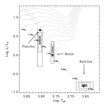
Figure 1.— H-R diagram showing evolution tracks (gray lines) and the true position of the three artificial stars (star symbols), which were not known by the hounds. The $1\sigma$, $2\sigma$, and $3\sigma$ error boxes show the positions of the stars according to the artificial “observed” traditional catalogue data, which were known by the hounds. For clarity we only show error boxes for cases K2, B2, and P2 (see Table 1). For details on how the catalogue data were generated see § 3.1.

For each star, 4-year time series were generated for all combinations of the following parameters: apparent magnitude $V=9,11,13,15$; inclination of rotation axis relative to the line of sight $i=0^{\circ},30^{\circ},60^{\circ}$; and rotation equal to one, two, and three times solar.

Figure 2.— Fourier spectra of 4-year Kepler time series of the artificial star Boris. Each panel corresponds to different apparent magnitudes, and shows co-added spectra from subdividing the time series in four day subsets. The large frequency spacing, $\Delta\nu$, between two modes of successive order $n$ is indicated in the top panel. The catalogue data for each case are shown in Table 1.

In Figure 2 we show four examples of power spectra for Boris ($V=9,11,13,15$). While the oscillations and the characteristic frequency spacing, $\Delta\nu$, are clearly seen for the brighter cases we can hardly see the excess power for the fainter ones. However, we saw from Chaplin et al. (2008) that the large frequency spacing can still be extracted in most cases in the tested magnitude range. The results from the exercise are shown in the last column of Table 1. We note that the ability to measure $\Delta\nu$ for the faintest case of Boris ($V=15$), and perhaps $V=13$, should be viewed with some caution. This is because the hounds in Exercise#1 had access to information about the frequency range in which they should measure $\Delta\nu$ from their analysis of the brighter cases where power excess is clearly visible. Hence, in a true blind case, as with real data, it might be harder to establish $\Delta\nu$ for such faint cases of ‘Boris-like’ stars. For the three faintest cases of Katrina ($V=11,13,15$) the large frequency spacing could not be determined, preventing an asteroseismic constraint on the radius.

Table 1Stellar input parameters given to each hound

		$V$	$\log g$		$T_{\mathrm{eff}}$	$\pi$	$\Delta\nu$
Case	Star	(mag)	(cm s-2)	$\log(Z/X)$	(K)	(mas)	($\mu$Hz)
K1	Katrina	9	4.8(.1)	-1.6(.1)	4505(200)	46.8(1.2)	227.82(.95)
K2	Katrina	9	4.8(.1)	-1.6(.1)	4505(100)	46.8(1.2)	227.82(.95)
B1	Boris	9	4.5(.1)	-1.6(.1)	5780(200)	12.5(1.2)	135.84(.49)
B2	Boris	9	4.5(.1)	-1.6(.1)	5780(25)	12.5(1.2)	135.84(.49)
B3	Boris	11	4.5(.1)	-1.6(.1)	5780(200)	5.4(2.2)	135.98(.59)
B4	Boris	11	4.5(.1)	-1.6(.1)	5780(25)	5.4(2.2)	135.98(.59)
B5	Boris	13	4.5(.1)	-1.6(.1)	5780(200)	3.9(3.6)	136.89(2.81)
B6	Boris	13	4.5(.1)	-1.6(.1)	5780(25)	3.9(3.6)	136.89(2.81)
B7	Boris	15	4.5(.1)	-1.6(.1)	5780(200)		141.94(2.43)
B8	Boris	15	4.5(.1)	-1.6(.1)	5780(25)		141.94(2.43)
P1	Pancho	9	4.3(.1)	-1.4(.1)	6383(200)	8.9(1.2)	69.74(.17)
P2	Pancho	9	4.3(.1)	-1.4(.1)	6383(40)	8.9(1.2)	69.74(.17)
P3	Pancho	11	4.3(.1)	-1.4(.1)	6383(200)	4.6(2.2)	69.74(.17)
P4	Pancho	11	4.3(.1)	-1.4(.1)	6383(40)	4.6(2.2)	69.74(.17)
P5	Pancho	13	4.3(.1)	-1.4(.1)	6383(200)	2.2(3.6)	69.75(.16)
P6	Pancho	13	4.3(.1)	-1.4(.1)	6383(40)	2.2(3.6)	69.75(.16)
P7	Pancho	15	4.3(.1)	-1.4(.1)	6383(200)		69.51(10.85)
P8	Pancho	15	4.3(.1)	-1.4(.1)	6383(40)		69.51(10.85)
P9	Pancho	15	4.3(.1)	-1.4(.1)	6383(200)		69.78(.33)
P10	Pancho	15	4.3(.1)	-1.4(.1)	6383(40)		69.78(.33)
K3	Katrina	9	4.8(.1)	-1.6(.1)	4505(200)	46.8(1.2)
K4	Katrina	9	4.8(.1)	-1.6(.1)	4505(100)	46.8(1.2)
B9	Boris	9	4.5(.1)	-1.6(.1)	5780(200)	12.5(1.2)
B10	Boris	9	4.5(.1)	-1.6(.1)	5780(25)	12.5(1.2)
B11	Boris	11	4.5(.1)	-1.6(.1)	5780(200)	5.4(2.2)
B12	Boris	11	4.5(.1)	-1.6(.1)	5780(25)	5.4(2.2)
B13	Boris	13	4.5(.1)	-1.6(.1)	5780(200)	3.9(3.6)
B14	Boris	13	4.5(.1)	-1.6(.1)	5780(25)	3.9(3.6)
B15	Boris	15	4.5(.1)	-1.6(.1)	5780(200)
B16	Boris	15	4.5(.1)	-1.6(.1)	5780(25)
P11	Pancho	9	4.3(.1)	-1.4(.1)	6383(200)	8.9(1.2)
P12	Pancho	9	4.3(.1)	-1.4(.1)	6383(40)	8.9(1.2)
P13	Pancho	11	4.3(.1)	-1.4(.1)	6383(200)	4.6(2.2)
P14	Pancho	11	4.3(.1)	-1.4(.1)	6383(40)	4.6(2.2)
P15	Pancho	13	4.3(.1)	-1.4(.1)	6383(200)	2.2(3.6)
P16	Pancho	13	4.3(.1)	-1.4(.1)	6383(40)	2.2(3.6)
P17	Pancho	15	4.3(.1)	-1.4(.1)	6383(200)
P18	Pancho	15	4.3(.1)	-1.4(.1)	6383(40)

The time-series data used in Exercise#1 were generated with the asteroFLAG simulator (Chaplin et al. 2009, in preparation). Each time series included photometric perturbations from p-modes, granulation, activity, photon noise, and instrumental noise. The stellar models were generated using the Aarhus stellar evolution code, ASTEC (Christensen-Dalsgaard, 2008b) using the simple but fast EFF equation of state (Eggleton et al., 1973) along with the Grevesse & Noels (1993) solar mixture using the OPAL tables at high temperature and the Kurucz (1991) table at lower temperature. The exact model values for $L$, $T_{\mathrm{eff}}$, and $R$ are listed in Table 2. The frequencies of the p-mode signal were calculated using the adiabatic pulsation code ADIPLS (Christensen-Dalsgaard, 2008a). The amplitude and damping rates were from semi analytical models (Chaplin et al., 2005). We refer to Chaplin et al. (2008) for further details on the simulations and Exercise#1 results.

3. Asteroseismic radius determination: Exercise#2

The aim of Exercise#2 is to use the large frequency spacings from Exercise#1, together with ‘traditional’ stellar parameters, to estimate the radii of the stars. While individual mode frequencies, and hence detailed asteroseismic analysis, are expected for the brighter stars, in this paper we only explore the benefit for the radius estimate from having access to the large frequency spacing. This work is an effort towards the development of robust algorithms for estimating radii of stars of different properties and noise levels in an automated pipeline fashion. It is the intention that the results are used to indicate what radius precision we can obtain on stars in the $V=9-15$ range, as will be observed by Kepler.

3.1. Stellar parameters

In addition to the large frequency spacing obtained from asteroseismology by the first group of hounds (Exercise#1), the second group of hounds (Exercise#2 – this paper) were given a set of traditional catalogue data for each star. These are given in Table 1. Each parameter, $\log g$, $\log(Z/X)$, $T_{\mathrm{eff}}$, and $\pi$ was obtained by adding to the true value (which the hounds did not know), a random number drawn from a normal distribution having zero mean and standard deviation equal to the adopted uncertainty on the parameter. Based on the traditional catalogue data we have estimated the locations of the stars in the H-R diagram, which are shown in Figure 1 together with the true values (star symbols). In reality most of the atmospheric parameters, such as $T_{\mathrm{eff}}$, $\log g$, and metallicity, will come from the Kepler Input Catalogue, which is based on calibrated photometry. However, for many of the most interesting targets the photometric information will be supplemented by high-resolution spectroscopy (Latham et al., 2005). Hence, for each star at each magnitude we analyzed two cases. In one, the uncertainty in $T_{\mathrm{eff}}$  was assumed to be $200\,$K, which is representative for the relevant stars from the Kepler Input Catalogue (T. M. Brown, priv. comm.). The other case assumed a smaller uncertainty in $T_{\mathrm{eff}}$, which would be the case if additional ground-based data, such as high-resolution spectra (Sousa et al., 2008), were available.

For the parallaxes we adopted Hipparcos-like precisions, with some extrapolation at the faint end to represent a conservative estimate of the expected astrometry from the Kepler data. For $V\gtrsim 13$ the Hipparcos-like parallaxes had large uncertainties, and we did not even generate predicted parallax data for $V=15$. For this faint end, the luminosity could only be estimated very roughly using the traditional stellar parameters.

The large frequency spacings quoted in Table 1 are the averages estimated from Exercise#1, and the uncertainties represent the scatter of the estimates. These values were made over results from all hounds on all datasets at each $V$ value. We recall that datasets in Exercise#1 were made for different internal rates of rotation, and different angles of inclination. Hence, the uncertainties given in Table 1 not only reflect the impact of reduction noise due to difference in analysis between hounds but also more subtle contributions from the different rotation and inclination.

For the faintest case of Pancho ($V=15$) there were outliers in the individual $\Delta\nu$ estimates returned by each hound in Exercise#1, and we decided to examine two versions of this star: one where $\Delta\nu$ was the mean of all the values returned by each hound, and the other where outliers were removed before calculating the mean.

Finally, we also considered cases for all stars where the large frequency spacing was not used by the hounds. These are listed in the bottom part of Table 1, below the line. This allowed us to compare the radius estimates with and without the asteroseismic constraint.

3.2. Analysis and results

Each hound in Exercise#2 worked independently and used different methods to determine the stellar radii. Details are given in § 4–8. All methods rely on matching various parameters (e.g. $L$, $Z$, $T_{\mathrm{eff}}$, and $\Delta\nu$) from stellar models with the corresponding observables (e.g. $V$, $\log g$, $\log(Z/X)$, $T_{\mathrm{eff}}$, $\pi$, and $\Delta\nu$) given in Table 1 to estimate the radius.

Table 2Results from the hounds

		$V$	$L_{\mathrm{model}}$	$T_{\mathrm{model}}$	$R_{\mathrm{model}}$	$R_{\mathrm{hound1}}$	$R_{\mathrm{hound2}}$	$R_{\mathrm{hound3}}$	$R_{\mathrm{hound4}}$	$R_{\mathrm{hound5}}$	$R_{\mathrm{hound6}}$
Case	Star	(mag)	$L_{\odot}$	(K)	$R_{\odot}$	$R_{\odot}$	$R_{\odot}$	$R_{\odot}$	$R_{\odot}$	$R_{\odot}$
K1	Katrina	9	0.15	4530	0.63	0.602(.012)	0.62(.01)	0.620(.004)	0.682(.007)
K2	Katrina	9	0.15	4530	0.63	0.610(.006)	0.61(.01)	0.627(.009)	0.627(.004)	0.62(.03)
B1	Boris	9	1.00	5778	1.00	0.977(.032)	1.02(.03)	1.007(.030)	1.007(.035)
B2	Boris	9	1.00	5778	1.00	0.993(.026)	1.01(.03)	0.990(.015)	1.017(.027)		1.036(.020)
B3	Boris	11	1.00	5778	1.00	0.957(.039)	1.01(.03)	0.984(.032)	1.010(.057)
B4	Boris	11	1.00	5778	1.00	0.993(.026)	1.01(.03)	0.988(.016)	1.028(.041)		1.035(.015)
B5	Boris	13	1.00	5778	1.00	0.965(.050)	1.00(.04)	0.975(.034)	1.012(.052)
B6	Boris	13	1.00	5778	1.00	1.002(.037)	1.00(.03)	0.984(.020)	1.023(.041)	0.93(.03)	1.029(.027)
B7	Boris	15	1.00	5778	1.00	0.936(.045)	0.97(.03)	0.956(.030)
B8	Boris	15	1.00	5778	1.00	0.971(.032)	0.97(.03)	0.958(.020)
P1	Pancho	9	4.53	6372	1.75	1.746(.046)	1.70(.04)	1.676(.033)	1.694(.051)
P2	Pancho	9	4.53	6372	1.75	1.709(.033)	1.70(.04)	1.749(.022)	1.709(.031)
P3	Pancho	11	4.53	6372	1.75	1.739(.049)	1.70(.05)	1.707(.049)	1.694(.051)
P4	Pancho	11	4.53	6372	1.75	1.764(.051)	1.70(.04)	1.754(.020)	1.709(.031)
P5	Pancho	13	4.53	6372	1.75	1.744(.051)	1.70(.05)	1.744(.044)	1.699(.060)
P6	Pancho	13	4.53	6372	1.75	1.764(.051)	1.70(.04)	1.757(.020)	1.715(.037)
P7	Pancho	15	4.53	6372	1.75	2.175(.328)		1.794(.225)
P8	Pancho	15	4.53	6372	1.75	2.197(.310)		1.731(.264)		1.70(.03)
P9	Pancho	15	4.53	6372	1.75	1.749(.055)	1.69(.05)	1.755(.036)	1.706(.067)
P10	Pancho	15	4.53	6372	1.75	1.765(.052)	1.71(.04)	1.755(.018)	1.744(.056)
K3	Katrina	9	0.15	4530	0.63	0.652(.075)	0.59(.01)	0.653(.022)
K4	Katrina	9	0.15	4530	0.63	0.652(.040)	0.59(.01)	0.657(.014)
B9	Boris	9	1.00	5778	1.00	1.169(.140)	1.04(.11)	1.173(.126)
B10	Boris	9	1.00	5778	1.00	1.169(.113)	1.00(.10)	1.152(.108)
B11	Boris	11	1.00	5778	1.00	1.077(.439)	0.94(.15)	1.098(.281)
B12	Boris	11	1.00	5778	1.00	1.077(.439)	0.92(.09)	1.094(.264)
B13	Boris	13	1.00	5778	1.00	0.594(.550)	0.71(.09)	0.915(.088)
B14	Boris	13	1.00	5778	1.00	0.594(.548)	0.92(.09)	0.931(.023)
B15	Boris	15	1.00	5778	1.00		0.71(.09)	1.366(.734)
B16	Boris	15	1.00	5778	1.00		0.92(.09)	1.383(.685)
P11	Pancho	9	4.53	6372	1.75	1.299(.193)	1.28(.15)	1.356(.150)
P12	Pancho	9	4.53	6372	1.75	1.300(.176)	1.28(.14)	1.336(.102)
P13	Pancho	11	4.53	6372	1.75	1.001(.483)	1.20(.18)	1.283(.143)
P14	Pancho	11	4.53	6372	1.75	1.001(.479)	1.22(.17)	1.297(.108)
P15	Pancho	13	4.53	6372	1.75	0.833(1.36)	1.19(.18)	1.347(.254)
P16	Pancho	13	4.53	6372	1.75	0.833(1.36)	1.22(.17)	1.293(.078)
P17	Pancho	15	4.53	6372	1.75		1.19(.18)	1.377(.502)
P18	Pancho	15	4.53	6372	1.75		1.22(.17)	1.294(.259)

In Table 2 we list the radius estimates returned by the hounds as well as the model values. Not all hounds examined all stars. By comparing the results from the top of the table (cases K1–2, B1–8, and P1–10) with those at the bottom (cases K3–4, B9–16, and P11–20) it is quite evident that including the large frequency spacing gives a significant improvement in our ability to determine the radius. In most cases, including this asteroseismic constraint reduces the uncertainty in the radius to a few percent, which is an improvement by a factor of 5–10. We note that in the bottom part of Table 2, the majority of the uncertainties from Hound-2 and a few from Hound-3, seem slightly underestimated compared to the deviations, $(R_{\mathrm{hound}}-R_{\mathrm{model}})/R_{\mathrm{model}}$, from the true value.

We summarize our main results in Figure 3. This shows the results listed in Table 2 for the stars that most hounds have examined, and which included the large frequency spacings. The uncertainties found by the hounds of roughly 1–3% generally seem to be consistent with the deviations that we see from the true values (see Fig. 3). We note a relatively small improvement in the radius estimates when the uncertainty in $T_{\mathrm{eff}}$ is significantly lower (left panels) than our base assumption of 200 K (right panels). This indicates that, provided we have the asteroseismic constraint (the large spacing), improving the estimate of $T_{\mathrm{eff}}$ is not particular important. In the following sections we discuss in more detail the methods adopted by the six hounds, and refer to § 9 for further discussion on how our results depend on the input parameters and their assumed uncertainties.

Figure 3.— Radii of the artificial stars and their $1\sigma$-error bars estimated by each hound are plotted in comparison with the true value indicated by the dashed lines. We show for each case the deviation in percent from the true value. Left panels show the results assuming $\sigma_{T_{\mathrm{eff}}}=200\,$K and right panels show more optimistic scenarios ($\sigma_{T_{\mathrm{eff}}}$(Katrina)$=100\,$K, $\sigma_{T_{\mathrm{eff}}}$(Boris)$=25\,$K, and $\sigma_{T_{\mathrm{eff}}}$(Pancho)$=40\,$K.)

4. RADIUS: Rapid Algorithm for Diameter Identification of Unclassified Stars (Hound-1)

In this section we describe the radius pipeline developed and utilized by DS to estimate stellar radii. The philosophy behind the development of this pipeline was to make it fast, robust and simple. It follows the same basic principle as the other methods described in the following sections, namely comparing a number of observables of a star with a grid of stellar models. All stellar models that are within $3\sigma$ of the observations in all four parameters $T_{\mathrm{eff}}$, $L$, $Z$, and $\Delta\nu$ simultaneously are treated as being equally likely. Hence, a model either fits (is within $3\sigma$) and is accepted or it does not fit, in which case it is discarded.

4.1. Models

The selection of models (step (2) below) was based on a model grid that covered uniformly the entire range ($\pm 3\sigma$) in $T_{\mathrm{eff}}$, $L$ and $Z/X$ spanned by each star (see Table 1). The resolution in $\log(Z/X)$ was 0.1 dex, corresponding to $\sigma_{\log(Z/X)}$, and the resolution in mass was $0.01\,M_{\odot}$. The grid was generated with the Aarhus stellar evolution code ASTEC using the simple but fast EFF equation of state (Eggleton et al., 1973), a fixed mixing-length parameter, $\alpha=1.8$, and an initial hydrogen abundance of $X=0.7$. We restricted the parameter space by fixing $\alpha$ and $X$. However, the effect of changing these parameters was explored by other hounds (see § 5, 7, and 8), who showed the effects to be quite small. The opacities were calculated using the solar mixture of Grevesse & Noels (1993) and the opacity tables of Rogers & Iglesias (1995) and Kurucz (1991) ($T<10\,000$ K). Rotation, overshooting and diffusion were not included. We used the adiabatic pulsation code ADIPLS to calculate $\Delta\nu$ for each stellar model.

4.2. Pipeline approach and results

The pipeline took the following approach:

1. It determined the location in the H-R diagram by calculating $L$ (Fig. 4; black cross and dotted 3-$\sigma$ error box). If the parallax was not known, as in the $V=15$ cases, the luminosity was estimated from $L/$L${}_{\odot}=(R/$R${}_{\odot})^{2}$($T_{\mathrm{eff}}$/$T_{\mathrm{eff}}$${}_{\odot})^{4}$, where $R/$R${}_{\odot}=(g/g_{\odot})/($$\Delta\nu$/$\Delta\nu$${}_{\odot})^{2}$.

2. It found the stellar models that matched within $\pm 3\sigma$ in $L$, $T_{\mathrm{eff}}$, $Z/X$, and $\Delta\nu$ (see Fig. 4; colored symbols).

3. Among all matching models, the two with the largest and the smallest radii, $R_{\mathrm{max}}$ and $R_{\mathrm{min}}$, were identified. Lines of constant radius with these values are shown in Figure 4 (dashed lines).

4. The estimated radius was calculated as the average: $R=\langle R_{\mathrm{max}},R_{\mathrm{min}}\rangle$, with uncertainty $\sigma_{R}=(R_{\mathrm{max}}-R_{\mathrm{min}})/6$ to accommodate that we found the two extreme models within $\pm 3\sigma$.

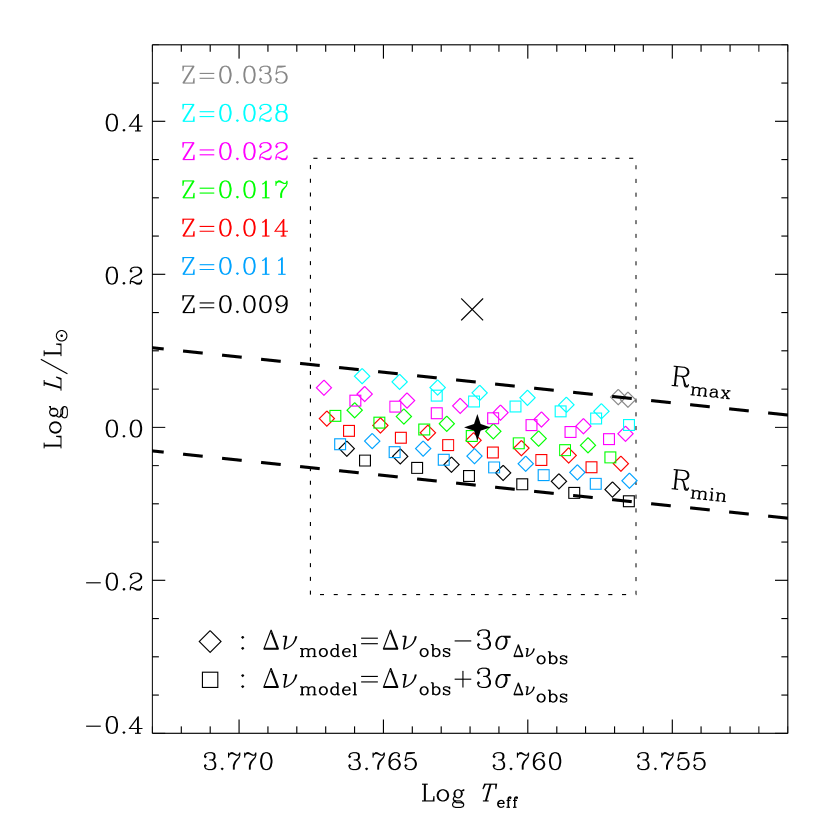
Figure 4.— Hound-1: Location of Boris (case B2) in the H-R diagram. The stellar location (cross) and $3\sigma$-error box (dotted) are shown in accord to the traditional catalogue data (see Table 1), while the true location of Boris is shown by the star symbol (not known by the hound). Colored symbols show the location of the stellar models with large frequency spacings that are equal to the observed value plus (squares) or minus (diamonds) $3\sigma$. The dashed lines indicate lines of constant radius for the largest and smallest model that agree with observations within $3\sigma$ in all four parameters: $L$, $T_{\mathrm{eff}}$, $Z$, and $\Delta\nu$. Note that models with fixed $Z$ and $\Delta\nu$ follow closely lines of constant radius.

In the following we give details for the two first steps:

1. To calculate $L$ we interpolated the grid of bolometric corrections by Lejeune et al. (1998), which takes the following input: $T_{\mathrm{eff}}$, $\log g$, and [Fe/H]. For that we first converted $Z/X$ to [Fe/H] using the solar values $Z_{\odot}=0.0188$ and $X_{\odot}=0.6937$ from Cox (2000). We further adopted M${}_{\mathrm{bol},\odot}=4.746$ from Lejeune et al. (1998). In the cases without parallax we used the solar values of $T_{\mathrm{eff}}$${}_{\odot}=5777\,$K, $\log g_{\odot}=4.44$ (Cox, 2000) and $\Delta\nu$${}_{\odot}=134.92\,$$\mu$Hz  (Toutain & Fröhlich, 1992) to estimate $L$.

2. To match models with observations we estimated $\Delta\nu$ by fitting to the radial modes of successive order $n$ in the frequency interval 0.75–1.25 times $\nu_{\mathrm{max}}$ (the frequency of highest power excess), which we estimated from scaling the solar value (see § 9 for a discussion on the best choice for the frequency range). The corresponding orders of $n$ for each star were: 19–33 (Katrina), 15–27 (Boris), 13–22 (Pancho). The calculation of $\Delta\nu$ was done for all models and the results stored in the grid, making the search for models that matched any given star extremely fast.

The results from this pipeline are summarised in Table 2 (column: Hound-1).

5. SEEK: A STATISTICAL APPROACH FOR THE AARHUS KEPLER PIPELINE (Hound-2)

Here we describe the results obtained by a beta version of the seek routine developed by POQ for the Aarhus Kepler pipeline. Like radius (§ 4), seek uses an extended grid of stellar models calculated with the Aarhus stellar evolution code (ASTEC) and the adiabatic pulsation code ADIPLS to estimate the radius of stars.

Like the radius procedure, the seek routine was developed for robustness, speed and simplicity, but we adopted a slightly more sophisticated approach. Instead of the brute force approach of radius, which simply selects all models within $3\sigma$ and calculates the radius as a simple average of the two extreme models (Fig. 4), seek selects the set of best-fitting models based on a $\chi^{2}$ formalism and estimates the radius by fitting a Gaussian to the distribution of radii of those models.

5.1. Models

The core of seek is the grid of models used to fit the observations. For this exercise we calculated and merged two regularly spaced subgrids, with various values for the mixing-length parameter and metallicity. The first subgrid comprised 20 sets of evolutionary tracks, each with a different combination of the mixing-length parameter in the range $1.2\leq\alpha\leq 3.0$ in steps of 0.6, and metallicity in the range $0.01\leq Z\leq 0.03$, in steps of 0.005. The second subgrid included 12 sets of tracks having $1.5\leq\alpha\leq 2.7$, and $0.0125\leq Z\leq 0.0275$, both with the same resolution as in the first grid. Each of the 32 sets comprised 57 evolution tracks from 0.6 to 3.0 $M_{\sun}$. The spacing between the tracks was 0.02 $M_{\sun}$ from 0.6 to 1.4 $M_{\sun}$ and 0.1 $M_{\sun}$ from 1.4 to 3.0 $M_{\sun}$.

In this beta version of the pipeline we used simple input physics to speed up the computation of the grid. In particular, the EFF equation of state (Eggleton et al., 1973) was used. The final version will use the modern OPAL equation of state, covering a more extended region of the metallicity and mixing-length parameter domains and include a range of hydrogen fractions, which in the current version was fixed at $X=0.7032$. The mixture of elements was taken from Grevesse & Noels (1993) and opacity tables were from the OPAL package supplemented by Ferguson et al. (2005) for low temperatures.

5.2. Method and results

We calculated the $\chi^{2}$ distribution of each star within our grid of models using:

$$\chi^{2}=\sum_{i=1}^{5}\left(\frac{O_{i}-M_{i}}{\sigma_{i}}\right)^{2},$$ (1)

where $O_{i}$ are the following five observed quantities: $\pi$, $T_{\mathrm{eff}}$, $\log g$, $\log(Z/X)$, and $\Delta\nu$, each with uncertainty $\sigma_{i}$ (see Table 1). The corresponding model quantities are $M_{i}$. In contrast to radius, seek does not estimate the observed luminosity to compare with the models, but instead calculates a model parallax to match the observed apparent magnitude of the star, which is assumed to be exact. The color transformation is done using the VandenBerg & Clem (2003) tables. In the faint cases ($V=15$) we had no parallax information, hence the parallax was not included in the $\chi^{2}$ sum. We derived the large frequency spacing for each model by fitting to successive radial overtones of order $n\geqq 15$ calculated with ADIPLS. These modes are in the asymptotic regime (Tassoul, 1980), meaning they are close to being equally spaced, and hence well suited for the computation of the large spacing (see § 9 for a discussion on the best choice for the frequency range of the modes for the $\Delta\nu$ calculation).

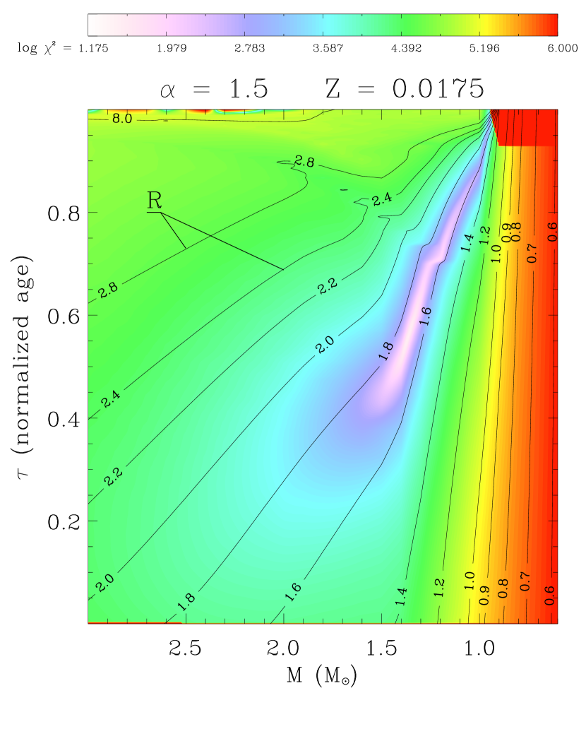
Figure 5.— Hound-2: $\chi^{2}$ calculated for Pancho (case P2) in the mass-age space for models with $Z=0.0175$ and $\alpha=1.5$. Radius contours are shown as solid lines (solar units). The color follows the $\log\chi^{2}$ as atop of the figure. $\tau$ is the age normalized by the age at the giant branch, thus stars evolve parallel to the ordinate from the Zero Age Main Sequence at $\tau=0$ to the giant branch at $\tau=1$. The kinks in the radius contours around $0.7\lesssim\tau\lesssim 0.9$ correspond to the blue hook in the H-R diagram. The dark red region in the upper right corner marks stars that are older than 14 Gyr.

A typical result of the $\chi^{2}$ calculation is shown in Figure 5 for Pancho ($V=9$). This illustrates a slice of the multidimensional parameter space with a fixed metallicity, $Z=0.0175$, and a fixed mixing-length parameter, $\alpha=1.5$. It shows clearly a valley of best-fitting models along a contour of constant radius (in this case $R\sim 1.7R_{\sun}$). While models with quite a range of masses and ages fit well to the observations, they all have roughly the same radius. However, due to a relatively flat bottom of the valley near the minimum there is no single best-fitting model. In other words the $\chi^{2}$ solution is degenerate. In addition, our grid has limited resolution and the $\chi^{2}$-minimization problem is highly nonlinear. Hence we cannot assume that the model with the lowest $\chi^{2}$ in the grid is the absolute minimum of the problem. Instead, we estimated the most likely value of the radius from a sample of best-fitting models for which $\chi^{2}$ was less than a given threshold, $\chi^{2}_{\rm th}$. We did this by first splitting the best-fitting models into bins of 0.005 $R_{\sun}$. For each bin we derived the total time spent by the models at that radius, which we denoted $t(R)$. This gave us the distribution, $t(R)$, of best-fitting radii, taking into account how likely it was to have the observed star at each particular radius.

If the threshold, $\chi^{2}_{\mathrm{th}}$, is well-chosen and the grid of models is dense enough to allow a large number of models to be within that threshold, $t(R)$ will be a normal distribution centred around the most likely value of the radius. We obtained the best value for $\chi^{2}_{\mathrm{th}}$ by an iterative process that minimized the difference between the median of the distribution, $t(R)$, and the centre of a Gaussian fit. In other words, we minimized the fitting error on the free parameter $R_{0}$, called $\Delta R_{0}$, by fitting the following Gaussian to the distribution $t(R)$ (see Fig. 6):

$$P(R;R_{0},\sigma)=\exp({-\frac{(R-R_{0})^{2}}{2\sigma^{2}}}),$$ (2)

where $R_{0}$ is our solution for the radius. We adopted $\sigma$ as the uncertainty on this radius, which of course was much larger than the fitting error, $\Delta R_{0}$ (see Press et al., 1992, for details on the fitting procedure). We note that our result is not highly sensitive to the choice of $\chi^{2}_{\mathrm{th}}$ as long as it is within a reasonable range of the best value. This is because the valley is relatively flat and has steep sides. However, if $\chi^{2}_{\mathrm{th}}$ is chosen excessively big or small it will change the width of the distribution, $t(R)$, and hence over- or underestimate the uncertainty on the radii.

The seek routine is able to establish the radius of the stars without requiring an intensive computation for every new star to be analyzed (a few seconds per star on an Intel Pentium D machine). Our results are presented in the Hound-2 column of Table 2.

5.3. Future development

If a given observable is not known, the extent of the grid will artificially set the minimum and maximum value of this observable. To take that into account, we will build our final grid to cover all reasonable values in metallicity, mixing length, and mass expected for solar-like stars. This constrained parameter space can be used to extract information about a star for which the only well known parameter is $\Delta\nu$. If we take a star with an uncertainty of $1\,$$\mu$Hz or less on $\Delta\nu$ and only assume that the star is located somewhere in the parameter space, we get a typical uncertainty of 5–10 % on the radius. This uncertainty is an absolute maximum if the large spacing is known. This capacity of providing a fast and reliable answer with minimum knowledge of the star is a powerful feature of the seek procedure.

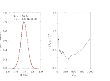
Figure 6.— Hound-2: Representation of the automatic seek process used to find stellar radii (Pancho; case P2). Left panel: Gaussian fit (red dashed line) to the distribution histogram $t(R)$ (black solid line), of the radii of the best-fitting models, which fulfil $\chi^{2}<\chi^{2}_{\mathrm{th}}=306$. The distribution has been normalized to unity. Right panel: Fitting error on $R_{0}$ as a function of the chosen threshold for selecting the best-fitting models. The red dot shows the threshold, $\chi^{2}_{\mathrm{th}}=306$ that results in the best fit.

6. The Shotgun method (Hound-3)

In this section we describe the automatic pipeline developed by HB, called shotgun, to perform radius estimation of stars with or without asteroseismic constraints. Similar to radius and seek, it uses a grid of stellar models, but differs by selecting a random sample of those models from which the radius is determined. While shotgun is still quite fast ($\sim 1\,$minute per star), it is somewhat slower than radius and seek. We note that the shotgun method is the only one presented here that does not make use of stellar pulsation calculations, but obtains the large spacing from scaling the solar value.

6.1. Models

We applied canonical scaled-solar BaSTI isochrones (Pietrinferni et al., 2004) in version $4.1.0$ with a mass-loss parameter $\eta=0.2$. The grid we used included stellar masses from $0.5$ to $5\,M_{\odot}$ with steps of typically $0.02\,M_{\odot}$ and metallicities from $Z=0.001$ to $0.04$. We converted the input parameter $\log(Z/X)$ to values of $Z$ by applying the hydrogen content of the Sun, $X_{\odot}=0.7395$, in agreement with $Y_{\odot}=0.2485$ (Basu & Antia, 2004) and $Z_{\odot}=0.012$ (Grevesse et al., 2007). Each model had a set of values $({\rm age},Z,M,L,T_{\rm eff})$ and for use in the following we calculated in addition $R/R_{\odot}=(T_{\rm eff}/T_{{\rm eff},\odot})^{-2}\,(L/L_{\odot})^{0.5}$ and the large spacing by scaling from the Sun, $\Delta\nu=\Delta\nu_{\odot}\,(M/M_{\odot})^{0.5}\,(R/R_{\odot})^{-1.5}$ (Kjeldsen & Bedding, 1995). For $\Delta\nu_{\odot}$ we used $134.8\,\mu$Hz from Kjeldsen et al. (2008).

6.2. Method and results

To select an unbiased sample of models from the discretely distributed BaSTI grid, shotgun first generates points from a non-discrete random distribution in the three-dimensional space $L$, $T_{\mathrm{eff}}$, and $\Delta\nu$, and finds the corresponding best matching models. The software is an IDL code that generates a ‘shot’ that is comprised of 50 randomly chosen three-dimensional points or ‘pellets’, $P_{i}=(L_{i},T_{{\rm eff,i}},\Delta\nu_{i}),i\in[1;50]$, with mean values and 1-$\sigma$ Gaussian random errors as listed in Table 1. The value of $L_{i}$ is calculated from the $V$ magnitude and the parallax, using bolometric corrections from Bessell et al. (1998), which depend mostly on $T_{\mathrm{eff}}$ and only weakly on $\log g$. When no parallax is available $L_{i}$ is ignored in equation (3) below. For each pellet the closest matching model in the BaSTI isochrones is found by identifying the highest value of the following weight function:

$$W_{i}=$$ (3)

$$\exp\left[-\frac{(L_{i}-L_{B})^{2}}{2\,\sigma^{2}_{L}}-\frac{(T_{{\rm eff},i}-T_{\rm eff,B})^{2}}{2\,\sigma^{2}_{T_{\rm eff}}}-\frac{(\Delta\nu_{i}-\Delta\nu_{B})^{2}}{2\,\sigma^{2}_{\Delta\nu}}\right]$$

where $B$ are the models in BaSTI. This is similar to finding the lowest $\chi^{2}$.

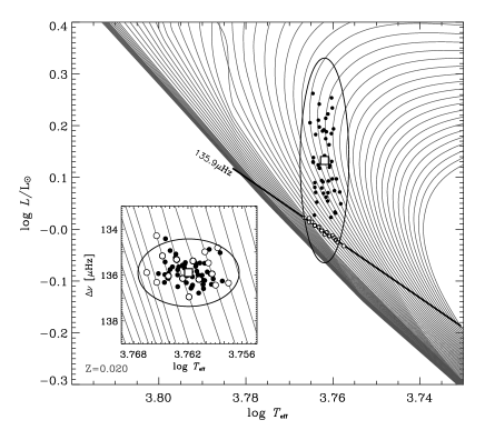
Figure 7.— Hound-3: H-R diagram showing isochrones from BaSTI for $Z=0.03$. The square symbol marks the input value for Boris (case B2) and the black dots are the 50 pellets generated by the shotgun software. The open circles mark the best model match for each pellet, defined as the highest value of the weights from Eq. 3. The 3-$\sigma$ error ellipse is indicated. The inset shows a similar diagram with $\Delta\nu$ vs. $T_{\mathrm{eff}}$.

We illustrate this in Figure 7, which shows an H-R diagram with BaSTI isochrones for metallicity $Z=0.03$. The large square and 3-$\sigma$ error ellipse represent Boris (case B2). The diagonal black line connects models on the BaSTI isochrones with the input large spacing of $135.9\,\mu$Hz. The solid circles are the 50 pellets generated by shotgun and the open circles mark were we find the highest value of the weights, $W_{i}$, for each pellet, hence representing the corresponding matched models. To illustrate all three parameters in Eq. 3 we show a similar diagram with the ordinate exchanged with the large spacing. It is clear that $\Delta\nu$ dominates the weight function in this example because the luminosity is very uncertain, which explains why all 50 pellets get matched to only 16 models within a narrow range apparently independent of the luminosity of the fired pellets. The output radius from shotgun is calculated as the mean value for the open circles in the BaSTI model grid while taking into account multiple hits on the same model, and the uncertainty is the 1-$\sigma$ RMS scatter. One could in principle include a term in Eq. 3 for the metallicity, but the BaSTI grid is too coarse in $Z$. Instead, we did the analysis for the two values of $Z$ in the grid that bracket the input value. Interpolating between the two values gave the final result for the radius, including the uncertainty associated with the uncertainty of $Z$. Our results are listed in Table 2 (Hound-3).

7. A global fitting approach (Hound-4)

We now proceed to describe the method used by OLC to estimate the stellar radii of Katrina, Boris, and Pancho. Like the seek procedure (§ 5), this approach is formulated as a $\chi^{2}$-minimization problem where the observations are used to find the best stellar model that minimizes equation (1). However, this approach differs by only using four observations in the $\chi^{2}$-minimization ($\Delta\nu$, $T_{\mathrm{eff}}$, $\log(Z/X)$, and $\log g$), while the apparent magnitude, $V$, and the parallax measurement, $\pi$, were used exclusively to estimate the mass range of the star.

7.1. Models

As is the case for seek and radius, the stellar models were derived using ASTEC and ADIPLS. The physics of the models included the OPAL95 opacity tables (Rogers et al., 1996) the mixing-length treatment of convection (Böhm-Vitense, 1958), with a fixed convective core overshoot parameter $d_{\mathrm{OV}}=0.25$, but variable mixing-length parameter, $\alpha$, nuclear energy generation rates, and the EFF equation of state (Eggleton et al., 1973).

7.2. Method

Unlike the previously described methods, we did not use a pre-calculated grid of models. Instead, the $\chi^{2}$ minimization was performed on one model at a time where derivative information was used to calculate the subsequent models that minimized the $\chi^{2}$, and so the only limitations in resolution were set by the output files of the models (e.g. five decimal places in solar radius). It has the advantage of not being limited by the parameter space of a grid including the flexibility of changing the input physics of the models. The disadvantage is that it needs to be run for various initial guesses to ensure a global minimum is found, with each run requiring new models to be calculated, which is more time consuming than the grid approach.

Because we only had four observations to estimate the five stellar model parameters (mass, age, $X$, $Z$, and $\alpha$), we had to fix one of the parameters, and we chose this to be $X$. In order to also explore the parameter $X$, the minimization was repeated while the fixed $X$ took values between 0.68 and 0.74 in steps of 0.01.

We use the Levenberg-Marquardt algorithm, along with singular value decomposition for the minimization (Press et al., 1992). The minimization is initiated giving each observed parameter, $O_{i}$, their uncertainties, ${\sigma_{i}}$, and an initial guess of the model parameters (mass, age, $X$, $Z$, and $\alpha$) as input. The solution is found when $\chi^{2}$ has reached 0.5 or after four iterations, which is sufficient for a stable solution. The frequency range used to derive $\Delta\nu$ of the model depended on the star and the magnitude. Examples for the $V=9$ cases are Katrina 6058–7915$\,\mu$Hz, Boris 2500–4100$\,\mu$Hz, and Pancho 1400–1978$\,\mu$Hz.

To avoid local minima problems, various runs were executed using different initial guesses of the mass, the range of which we estimate by deriving $M_{V}$ from $V$ and $\pi$ and subsequently using the relations between $M_{V}$ and mass from Allen (1973). The scheme automatically found the stellar model that minimized $\chi^{2}$ for each initial guess. Because we had various runs of the minimization with different initial masses ($N_{M}$) and different initial $X$ values ($N_{X}$), we essentially ran $N_{M}\times N_{X}$ minimizations and thus obtained this same number of best-fitting models (see Figs 8 and 9). We determined the radius of each of the best-fitting models and chose the radius values from the models whose $\chi^{2}$ is below a suitable threshold. These models correspond to the filled circles in Figures 8 and 9. The quoted radius in Table 2 is the mean value of these, while the uncertainty is defined as half of the difference between the largest and smallest radius value.

7.3. Results

Figure 8 shows examples of the masses and ages of the best-fitting models for various runs for Pancho ($V$=9). The initial guesses of the mass were 1.25, 1.30, 1.35, and 1.40 M_⊙, while the $X$ value was also changed for each run. There are a total of 4 x 7 minimizations, and therefore we have a total of 28 best-fitting models, each represented by a circle whose size is inversely proportional to the $\chi^{2}$ value as defined by equation (1) (i.e. a larger point means a better fit). The filled circles are those models that give a $\chi^{2}<3.9^{2}$. For each (almost vertical) ridge in Figure 8, $X$ varies between 0.68 and 0.74. The dotted lines connects the results for $X=0.69,0.71$ and $0.73$. By inspecting the figure, it is clear that there are correlations among the parameters, meaning that we can obtain the same $\chi^{2}$ value (same dot size in Fig. 8) for a range of parameter combinations. The filled circles are those models that we accept as the best models, but still mass, age and $X$ span large parameter ranges. This clearly demonstrates that some of the global parameters cannot be significantly constrained by the observations that we have available in this exercise. For example, we can see the age of the best-fitting models varies between a significant range of 1.4 and 2.1 Gyr, and the mass varies from about 1.30 to 1.45 M_⊙. In fact, the 1-$\sigma$ uncertainties on the model with the lowest $\chi^{2}$ value are $\sigma(\mathrm{Mass})$ = 5% , $\sigma(\mathrm{age})$ = 21%, $\sigma(Z)$ = 23% and $\sigma(\alpha)$ = 10%.

Figure 8.— Hound-4: Best-fitting parameters of mass and age for various minimization runs for Pancho (case P2). The larger circles represent the models with the lower $\chi^{2}$ values. The filled circles represent the models whose $\chi^{2}<3.9^{2}$. The dotted lines connect the results for selected values of $X$.

Figure 9.— Hound-4: Radius and effective temperature for the same models as in Figure 8. The dotted line is the observed $T_{\rm eff}$.

In Figure 9 we show the corresponding radii and effective temperatures of the same models as shown in Figure 8. The dotted line indicates the observed $T_{\rm eff}$. All of the models fall within $\pm 3\sigma_{T_{\rm eff}}$. In agreement with the results we found using seek and radius most of these models have roughly the same radius despite spanning a large parameter range in mass, $X$, and age.

This automatic minimization scheme was repeated for each of the stars and for each $V$ value, and the results are listed in Table 2 (column Hound-4).

8. Non automated approaches

While the four methods described in the previous sections (§ 4–7) were all automated, three relying on large existing grids of stellar models, we now turn to methods that involve generating small sets of models covering more limited ranges of the parameter space, and iteratively narrowing down the parameter space of best-fitting models manually. The fundamental idea – fitting model parameters to observations – is still the same, but instead of being developed to the level of fast pipeline algorithms, which can be applied routinely on large sets of stars, the following methods again serve to demonstrate the ability to determine precise radii. In addition, these methods use different stellar evolution and pulsation codes to those in § 4–7, allowing a valuable comparison.

8.1. The Granada approach (Hound-5)

In this section we present the methodology adopted by JCS, AM, and AGH to estimate the radii of the three artificial stars (see Table 1). In contrast to the other hounds, we did not use the apparent magnitude and the parallax information. We therefore have only one case for each star, for which we adopted the average large spacing and the largest uncertainty listed in Table 1 (case K2, B6, and P8).

8.1.1 Modelling

To model the stars we constructed standard non-rotating models from late pre-main-sequence to terminal-age main sequence (where core hydrogen fusion ceases). We note that this does not cover all evolution states that are consistent with the observed parameters and their error bars, especially for Pancho, and our results may therefore have systematic errors. The evolutionary stellar models were computed with the CESAM code (Morel, 1997). Opacity tables were taken from the OPAL package (Iglesias & Rogers, 1996), complemented at low temperatures ($T\leq 10^{4}\,$K) by the tables by Alexander & Ferguson (1994). The atmosphere was constructed from a grey Eddington $T-\tau$ relation (Eddington, 1926). Convection was treated with a local mixing-length model (Böhm-Vitense, 1958) and we assumed various values for the mixing-length parameter $\alpha=l/H_{\rm p}$, where $l$ is the mixing length and $H_{\rm p}$ is the pressure scale height. In particular, values between 0.5 and 2 were explored. For the overshoot parameter $d_{\rm OV}=l_{\rm OV}/H_{\rm p}$ ($l_{\rm OV}$ being the penetration length of the convective elements) we assumed values between 0.0 and 0.3. Such ranges of parameters cover the range of parameters generally adopted for solar-like stars.

For the computations of adiabatic eigenfrequencies two oscillation codes were used: FILOU (Tran Minh & Léon, 1995; Suárez, 2002; Suárez & Goupil, 2008) and GraCo (Moya et al., 2004; Moya & Garrido, 2008).

8.1.2 Method

First, we calculated about 30 initial models that covered the observed $\pm 3\sigma$ range of each parameter, $\log g$, $\log(Z/X)$, and $T_{\mathrm{eff}}$, while making sure they also covered various values of mixing length and overshoot. From those initial models we then selected 3–5 representative models with various masses and evolution states for which the large spacing was also within $3\sigma$ of the observed value. The exact number of representative models varied from star to star. We consider the large spacing as the strongest bound on the radius. Hence, in order to get a better radius estimate we made an additional 3–4 models around each representative model, which were then all within $3\sigma$ of the observed $\log g$, $\log(Z/X)$, $T_{\mathrm{eff}}$, and $\Delta\nu$, with the majority within $1\sigma$ of the latter. This provided a total of about 9–20 representative models. Our final estimate of the radius (Table 2, column Hound-5) is a simple average of the radii of those representative models ($R=\langle R_{\mathrm{model}}\rangle$) and the corresponding uncertainty is the maximum deviation from the mean ($\sigma_{R}=\mathrm{MAX}(R_{\mathrm{model}}-\langle R_{\mathrm{model}}\rangle)$).

8.2. The CAUP approach (Hound-6)

In this section we describe the procedure used by SGS and MJPFGM to estimate stellar radii. This approach is similar to the one described in § 8.1, in that an initial set of stellar models was made based on the observed parameters and their uncertainties. Then, by testing which models fit best (in the $\log g$, $L$, $T_{\mathrm{eff}}$ parameter space), further refinement of the range of parameter values were made by calculating additional models. Finally pulsation models were derived to further constrain the parameter space using the strong bound from $\Delta\nu$.

Of the 13 stellar cases listed in Table 1, the procedure described here was only applied on one star (Boris, case B2, B4, and B6). The method does not rely on a pipeline algorithm, but can be improved and used for all the stars. Unlike the methods described in the previous sections, this approach only considered stellar models to be valid if they were within one sigma of the observed $\log g$, $L$, and $T_{\mathrm{eff}}$ simultaneously.

8.2.1 Models

To obtain the evolution tracks we used the CESAM code version 2K (Morel, 1997; Morel & Lebreton, 2008). The Livermore radiative opacities were used (Iglesias & Rogers, 1996) complemented at low temperatures ($T\leq 10^{4}\,$K) by atomic and molecular opacity tables from Kurucz (1991). The opacities were calculated with the solar mixture of Grevesse & Noels (1993), convection was described by the mixing length model (Böhm-Vitense, 1958), and overshooting ($d_{\mathrm{OV}}$) was not used since this parameter is poorly known, in particular for stars below $2\,$M_⊙ (Ribas et al., 2000). The nuclear reaction rates were from the Nuclear Astrophysics Compilation of REaction Rates (NACRE) (Angulo et al., 1999). For the equation of state the OPAL 2005 tables were used. The atmosphere of the stellar models was based on a Hopft law (Mihalas, 1978) where convection was not included, and radiative transfer was considered to be independent of the radiation frequency (i.e. the grey case was assumed). We derived frequencies of the models with the pulsation code POSC (Monteiro, 2008)

8.2.2 Method

By using the parameters in Table 1 we located the star and its 1-$\sigma$ error box in both the H-R and $\log g$ vs. $T_{\mathrm{eff}}$  diagrams. To locate the position in the H-R diagram we estimated the stellar luminosity, computed from the parallax and the apparent magnitude, using the calibration by Flower (1996) to obtain the bolometric correction. In the calculation we adopted the solar absolute magnitude of M_V = 4.81 (Bessell et al., 1998) and a bolometric correction for the Sun of 0.08 mag (Flower, 1996). The uncertainty on the luminosity comes mainly from the parallax. We then built a grid of stellar models, for different masses, $M$, initial helium content, $Y_{0}$, and mixing length, $\alpha$, while having the initial metallicity ratio $Z_{0}/X_{0}$ fixed and equal to the observed $Z/X$.

Table 3Stellar model grids (Hound-6)

Grid	1				2			3				4					5
$M/$M⊙	0.94	0.97	1.03	1.06	1.02	1.03	1.04		1.08	1.10	1.12	1.11	1.12	1.13	1.14		1.08	1.09	1.10
$Y_{0}$	0.24	0.26	0.28	0.30	0.25	0.26	0.27	0.24	0.26	0.28	0.30	0.23	0.24	0.25	0.26	0.27	0.23	0.24	0.25	0.26
$\alpha$	1.20	1.40	1.60	1.80	1.50	1.60	1.70	1.20	1.40	1.60	1.80	1.30	1.40	1.50	1.60		1.30	1.40	1.50	1.60	1.70	1.80

In the following we use Boris (case B2) as an example to describe the process of finding valid fitting models.

In an iterative process, we calculated three grids of models (see Table 3; grid 1, 2, and 3) to determine the range in $M$, $Y_{0}$, and $\alpha$, that made the models fall within $\pm 1\sigma$ of the observed $\log g$, $T_{\mathrm{eff}}$, and $L$, simultaneously. In this process we made evolution tracks with all the possible combinations of $M$, $Y_{0}$, and $\alpha$ within each grid. We finally computed two more grids (4 and 5) with higher resolution but covering roughly the same parameter space as the third grid. With our adopted fixed ratio $\log(Z_{0}/X_{0})=-1.6$, the range in $Y_{0}$ corresponded to $Z_{0}=0.017$–0.019, and $X_{0}=0.68$–0.75. We note that this is a relatively small change in metallicity compared to the uncertainty quoted in Table 1. Hence, it is possible that we do not see the full effect on our radius estimate from the uncertainty in the metallicity.

From all the grids, roughly 300 models from 32 tracks were within $\pm 1\sigma$ in $\log g$, $\log L$, and $T_{\mathrm{eff}}$ simultaneously. From this selection of models we picked one reference model on each track, and compute the pulsation frequencies in order to obtain the large frequency spacings, $\Delta\nu$, which we derived by fitting successive radial overtones in the frequency range 2400–4000$\,\mu$Hz. Depending on the models the corresponding radial orders fell in the range $n=16$–30. To save time computing pulsations models, we estimated $\Delta\nu$ for the rest of the models along each track using the following scaling relation:

$$\Delta\nu=(M/M_{\mathrm{ref}})^{1/2}(R/R_{\mathrm{ref}})^{-3/2}\Delta\nu_{\mathrm{ref}},$$

where $\Delta\nu_{\mathrm{ref}}$, $M_{\mathrm{ref}}$, $R_{\mathrm{ref}}$ are the large frequency spacing, the mass, and the radius of the respective reference model.

We finally selected the best two thirds of the models (188 models in the case B2), which showed the smallest deviation between our estimated large spacing and the observed value.

Figure 10.— Hound-6: Radius vs. large spacing for the 188 best-fitting models within one sigma in $\log g$, $\log L$, and $T_{\mathrm{eff}}$ (Boris, case B2). The vertical line shows the measured $\Delta\nu$ and the horizontal line is the corresponding radius found by this approach.

In Figure 10 we plot the relation between the large spacing and the radius for those models. We made a simple linear fit to the points presented in Figure 10 and used it to estimate the radius of the star, by evaluating the value of the fit at the observed large spacing (see vertical and horizontal lines in Figure 10).

To estimate the uncertainty on the radius we combined the uncertainty from the fit and the uncertainty in the observed large frequency spacing. We obtained the latter by multiplying the uncertainty on the observed large frequency spacing with the slope of the fit. The uncertainty from the other observables are included in the uncertainty of the fit, since the points used for the fitting were obtained considering all models within the error boxes. The results for the cases B2, B4, and B6 can be seen in Table 2 (column Hound-6).

9. Discussion

In this section we will discuss how our radius estimates are constrained by our input parameters and their associated uncertainties. We further discuss the possible systematic errors in the results.

9.1. Dependencies on input parameters

Figure 4, which is the output from the radius pipeline, illustrates to some extent the effects of the various input parameters. All models that agree with the observations within $3\sigma$ (colored symbols) are bound by $T_{\mathrm{eff}}$, $\Delta\nu$, and the metallicity. The gravity and parallax (when available) are in general so uncertain that they do not constrain the luminosity enough to exclude any models not already excluded by $T_{\mathrm{eff}}$, $\Delta\nu$, and the metallicity. Only in a few of the brightest cases ($V=9$) does the parallax exclude some additional models, reducing $\sigma_{R}$ slightly. Hence, despite the increasing uncertainty in the luminosity for the fainter stars we basically get the same radius and $\sigma_{R}$ (see Table 2). It is in fact mostly the increase in $\sigma_{\Delta\nu}$ that is responsible for the slight increase in $\sigma_{R}$ towards fainter stars. The redundancy of $\log g$ is further confirmed by re-running the analysis for a few of the stars with increased uncertainty $\sigma_{\log g}=0.2$, and again we obtain the same results within the uncertainty.

Again, if we use Figure 4 as illustration we see that $\sigma_{\Delta\nu}$ and $\sigma_{T_{\mathrm{eff}}}$ contribute roughly equally to the uncertainty in the radius. However, it is evident that the largest contribution comes from the uncertainty in the metallicity. It is $\sigma_{\log(Z/X)}$ that is responsible for increasing the acceptable range of radius values. It will therefore require a much lower $\sigma_{T_{\mathrm{eff}}}$ and $\sigma_{\pi}$ to reduce $\sigma_{R}$ by the same amount as we will achieve by a slightly better determined metallicity. We regard the applied $\sigma_{\log(Z/X)}=0.1$ as realistic, but if one can reduce the uncertainty in the observed metallicity by a factor of two to four, we can reduce the uncertainty in the radius down to $\sim 1\%$, depending on the position of the star in the H-R diagram. Only in the case of a very poorly determined $\Delta\nu$ does $\sigma_{\Delta\nu}$ contribute more than $\sigma_{\log(Z/X)}$ to the final $\sigma_{R}$ (see Table 2; cases P7 and P8).

We further note from Figure 4 that the models of constant $\Delta\nu$ for a fixed metallicity, say the black squares, run almost parallel to lines of constant radius (dashed). This explains why decreasing $\sigma_{T_{\mathrm{eff}}}$ has so little effect on $\sigma_{R}$ (see Table 2; cases B1, B3, B5, and B7 versus B2, B4, B6, and B8). This parallel alignment is even more pronounced for the hotter star Pancho, which therefore shows no decrease in $\sigma_{R}$ as we decrease $\sigma_{T_{\mathrm{eff}}}$. For the cooler star Katrina, the alignment is not as good, and a better-determined $T_{\mathrm{eff}}$ does improve the radius estimate. A similar illustration is shown in Figure 5, which shows that the best fitting models (low $\chi^{2}$) lie along contours of constant radius despite having a large range in age and mass. The tight correlation between $R$ and $\Delta\nu$ seen in Figure 10 further illustrates that this relation is not strongly dependent on the initial physics (mass, mixing length, initial helium abundance) of the star, which underpins that $\Delta\nu$ is a powerful measure to constrain the stellar radius.

In summary, provided we have access to the large spacing, only metallicity and to less extent $T_{\mathrm{eff}}$ provide additional constraints to the radius, while the parallax and $\log g$ are redundant due to their large uncertainties.

9.2. Systematic errors

For a given star, the large spacing is not strictly the same at all frequencies in the p-mode spectrum, but varies smoothly with frequency. Hence, to correctly compare observations and models, it is necessary to use the same frequency range in both cases when $\Delta\nu$ is derived. However, this was not attainable in this study because the adopted observed large spacing was the average of all values returned by each hound of the previous Exercise#1, each of whom used different frequency ranges. Fortunately, it is straightforward to employ a common frequency range for the observations and the models in the final pipeline for analyzing real Kepler data.

We further note that all hounds used only the radial modes to derive $\Delta\nu$ from the models, while the observed values included information on all detectable modes. This introduced a systematic error on the radius measurement because modes of different angular degree $l$ have slightly different spacings. For a solar model this difference is 0.5% at most. Since $\Delta\nu$ $\propto\rho^{0.5}$ we can get a rough estimate of the corresponding systematic error on the radius of $<0.3$%. However, this again can be corrected for and the effect be eliminated.

When fitting stellar evolution tracks to the stellar location in the H-R diagram, a common strategy is to restrict the search to the 1-$\sigma$ error box ($L$, $T_{\mathrm{eff}}$). Our investigation clearly shows that this approach can lead to wrong results. With the very precise measurements of $\Delta\nu$, we saw stars where traditional parameter values (e.g. $L$, $T_{\mathrm{eff}}$) would deviate by more than 1$\sigma$, in order to match $\Delta\nu$ within 3$\sigma$, which explains why some of the stars fall outside their 1-$\sigma$ error box in Figure 1. Statistically this is of course not surprising, but we still find it important to stress the point.

In addition to the statistical aspect, inconsistencies can arise if there are systematic differences between the physics included in the modeling of the hares and the hounds or between the real star and the models. The stellar model codes used by the hares and hounds have been developed over many years and are well tested. For example, these codes have been shown to give almost the same radii and luminosities, with differences on the order of 0.05% (Lebreton et al., 2008). Further, comparing results from the various hounds suggest that the detailed input physics has a relatively small effect on the radius estimate. Recently, Kjeldsen et al. (2009) suggested that the well-known offset of roughly 1% between the observed $\Delta\nu$ of the Sun and the value derived from stellar models, which comes from improper modeling of the near-surface layers of the Sun, can be corrected for empirically. This offset, which is likely to affect models of other stars as well, has not been accounted for in this investigation because it requires knowledge of individual mode frequencies. The systematic effect on the asteroseismic radius estimate from this offset is therefore expected to be roughly 0.7% for a Sun-like star.

Finally, we note that the hounds were given $\log(Z/X)$ and their results therefore did not depend on the adopted solar value to any large degree. However, in reality one needs to convert the observed metallicity to $X$, $Y$, and $Z$ to compare with the models, and this conversion depends on the assumed solar metallicity. The range of $Z_{\odot}$ values currently accepted, $0.012\lesssim Z_{\odot}\lesssim 0.017$ (Grevesse et al., 2007; Caffau et al., 2008) will correspond to the same range in $Z$ for a star similar to the Sun. This change, $\Delta Z=0.005$, will change the estimated radius by about 1–2%.

10. Conclusions

In an extensive hare-and-hounds exercise, we have analyzed artificial solar-type main-sequence stars, which are representative for targets observed during the Kepler mission. The stellar radii found by each hound, using different approaches and codes for stellar evolution and pulsation calculations, are in good agreement with one another and with the true values.

We are able to determine the radius with a precision of a few percent, and are confident that radii can be obtained with $<3$% accuracy for solar-like Kepler targets on a routine basis using automatic pipeline reduction. We demonstrate that the reason for this is the strong relation between the radius and the large frequency spacing, which can be measured to very high accuracy. Our results further show that the radius is only weakly dependent on the input physics of the stellar models, including the equation of state and the mixing-length parameter.

The uncertainty in the radius determination is mostly dominated by the uncertainty in the stellar metallicity, which translates to an uncertainty in the stellar mass. In most cases the parallax and the surface gravity are too uncertain to constrain the radius, so in essence only the uncertainty in effective temperature and the large frequency spacing adds further to the final uncertainty in the radius. However, we conclude that we do not need to know $T_{\mathrm{eff}}$ to a very high precision in order to obtain a good estimate of the radius, provided we have access to $\Delta\nu$.

Because the Kepler mission will provide high accuracy data for many binary systems, there will be cases where we will obtain both an ‘asteroseismic radius’, and a ‘photometric radius’ giving opportunities to independently test the accuracy of our radius estimates.

While these results rely on 4-yr time series, similar results are expected from time series of only 1–3 months but with a limiting magnitude of about $V\sim 11$. Details on limiting magnitudes for determination of the various frequency spacings is the aim of ongoing asteroFLAG exercises.

References

- Alexander & Ferguson (1994) Alexander, D. R., & Ferguson, J. W. 1994, ApJ, 437, 879
- Allen (1973) Allen, C. W. 1973, Astrophysical quantities (London: University of London, Athlone Press, —c1973, 3rd ed.)
- Angulo et al. (1999) Angulo, C., Arnould, M., Rayet, M., Descouvemont, P., Baye, D., Leclercq-Willain, C., Coc, A., Barhoumi, S., Aguer, P., Rolfs, C., Kunz, R., Hammer, J. W., Mayer, A., Paradellis, T., Kossionides, S., Chronidou, C., Spyrou, K., Degl’Innocenti, S., Fiorentini, G., Ricci, B., Zavatarelli, S., Providencia, C., Wolters, H., Soares, J., Grama, C., Rahighi, J., Shotter, A., & Lamehi Rachti, M. 1999, Nuclear Physics A, 656, 3
- Appourchaux et al. (2008) Appourchaux, T., Michel, E., Auvergne, M., Baglin, A., Toutain, T., Baudin, F., Benomar, O., Chaplin, W. J., Deheuvels, S., Samadi, R., Verner, G. A., Boumier, P., García, R. A., Mosser, B., Hulot, J.-C., Ballot, J., Barban, C., Elsworth, Y., Jiménez-Reyes, S. J., Kjeldsen, H., Régulo, C., & Roxburgh, I. W. 2008, A&A, 488, 705
- Baglin et al. (2006) Baglin, A., Auvergne, M., Boisnard, L., Lam-Trong, T., Barge, P., Catala, C., Deleuil, M., Michel, E., & Weiss, W. 2006, in COSPAR, Plenary Meeting, Vol. 36, 36th COSPAR Scientific Assembly, 3749
- Basu & Antia (2004) Basu, S., & Antia, H. M. 2004, ApJ, 606, L85
- Bessell et al. (1998) Bessell, M. S., Castelli, F., & Plez, B. 1998, A&A, 333, 231
- Böhm-Vitense (1958) Böhm-Vitense, E. 1958, Zeitschrift fur Astrophysik, 46, 108
- Borucki et al. (2008) Borucki, W., Koch, D., Basri, G., Batalha, N., Brown, T., Caldwell, D., Christensen-Dalsgaard, J., Cochran, W., Dunham, E., Gautier, T. N., Geary, J., Gilliland, R., Jenkins, J., Kondo, Y., Latham, D., Lissauer, J. J., & Monet, D. 2008, in IAU Symposium, Vol. 249, IAU Symposium, 17
- Brown et al. (2005) Brown, T. M., Everett, M., Latham, D. W., & Monet, D. G. 2005, in Bulletin of the American Astronomical Society, Vol. 37, Bulletin of the American Astronomical Society, 1340
- Caffau et al. (2008) Caffau, E., Ludwig, H.-G., Steffen, M., Ayres, T. R., Bonifacio, P., Cayrel, R., Freytag, B., & Plez, B. 2008, A&A, 488, 1031
- Chaplin et al. (2008) Chaplin, W. J., Appourchaux, T., Arentoft, T., Ballot, J., Christensen-Dalsgaard, J., Creevey, O. L., Elsworth, Y., Fletcher, S. T., García, R. A., Houdek, G., Jiménez-Reyes, S. J., Kjeldsen, H., New, R., Régulo, C., Salabert, D., Sekii, T., Sousa, S. G., Toutain, T., & the rest of the asteroFLAG group. 2008, Astronomische Nachrichten, 329, 549
- Chaplin et al. (2005) Chaplin, W. J., Houdek, G., Elsworth, Y., Gough, D. O., Isaak, G. R., & New, R. 2005, MNRAS, 360, 859
- Christensen-Dalsgaard (2008a) Christensen-Dalsgaard, J. 2008a, Ap&SS, 316, 113
- Christensen-Dalsgaard (2008b) —. 2008b, Ap&SS, 316, 13
- Christensen-Dalsgaard et al. (2007) Christensen-Dalsgaard, J., Arentoft, T., Brown, T. M., Gilliland, R. L., Kjeldsen, H., Borucki, W. J., & Koch, D. 2007, Communications in Asteroseismology, 150, 350
- Cox (2000) Cox, A. N. 2000, Allen’s astrophysical quantities (Allen’s astrophysical quantities, 4th ed. Publisher: New York: AIP Press; Springer, 2000. Editedy by Arthur N. Cox. ISBN: 0387987460)
- Eddington (1926) Eddington, A. S. 1926, The Internal Constitution of the Stars (The Internal Constitution of the Stars, Cambridge: Cambridge University Press, 1926)
- Eggleton et al. (1973) Eggleton, P. P., Faulkner, J., & Flannery, B. P. 1973, A&A, 23, 325
- Ferguson et al. (2005) Ferguson, J. W., Alexander, D. R., Allard, F., Barman, T., Bodnarik, J. G., Hauschildt, P. H., Heffner-Wong, A., & Tamanai, A. 2005, ApJ, 623, 585
- Flower (1996) Flower, P. J. 1996, ApJ, 469, 355
- Grevesse et al. (2007) Grevesse, N., Asplund, M., & Sauval, A. J. 2007, Space Science Reviews, 130, 105
- Grevesse & Noels (1993) Grevesse, N., & Noels, A. 1993, in Origin and Evolution of the Elements, ed. S. Kubono & T. Kajino, 14
- Iglesias & Rogers (1996) Iglesias, C. A., & Rogers, F. J. 1996, ApJ, 464, 943
- Kjeldsen & Bedding (1995) Kjeldsen, H., & Bedding, T. R. 1995, A&A, 293, 87
- Kjeldsen et al. (2008) Kjeldsen, H., Bedding, T. R., & Christensen-Dalsgaard, J. 2008, ApJ, 683, L175
- Kjeldsen et al. (2009) Kjeldsen, H., Bedding, T. R., & Christensen-Dalsgaard, J. 2009, in IAU Symposium, Vol. 253, IAU Symposium, 309–317
- Kurucz (1991) Kurucz, R. L. 1991, in NATO ASIC Proc. 341: Stellar Atmospheres - Beyond Classical Models, 441
- Latham et al. (2005) Latham, D. W., Brown, T. M., Monet, D. G., Everett, M., Esquerdo, G. A., & Hergenrother, C. W. 2005, in Bulletin of the American Astronomical Society, Vol. 37, Bulletin of the American Astronomical Society, 1340
- Lebreton et al. (2008) Lebreton, Y., Montalbán, J., Christensen-Dalsgaard, J., Roxburgh, I. W., & Weiss, A. 2008, Ap&SS, 316, 187
- Lejeune et al. (1998) Lejeune, T., Cuisinier, F., & Buser, R. 1998, A&AS, 130, 65
- Mihalas (1978) Mihalas, D. 1978, Stellar atmospheres 2nd edition (San Francisco, W. H. Freeman and Co., 1978. 650 p.)
- Monteiro (2008) Monteiro, M. J. P. F. G. 2008, Ap&SS, 316, 121
- Morel (1997) Morel, P. 1997, A&AS, 124, 597
- Morel & Lebreton (2008) Morel, P., & Lebreton, Y. 2008, Ap&SS, 316, 61
- Moya & Garrido (2008) Moya, A., & Garrido, R. 2008, Ap&SS, 316, 129
- Moya et al. (2004) Moya, A., Garrido, R., & Dupret, M. A. 2004, A&A, 414, 1081
- Pietrinferni et al. (2004) Pietrinferni, A., Cassisi, S., Salaris, M., & Castelli, F. 2004, ApJ, 612, 168
- Press et al. (1992) Press, W. H., Teukolsky, S. A., Vetterling, W. T., & Flannery, B. P. 1992, Numerical recipes in C. The art of scientific computing (Cambridge: University Press, —c1992, 2nd ed.)
- Ribas et al. (2000) Ribas, I., Jordi, C., & Giménez, Á. 2000, MNRAS, 318, L55
- Rogers & Iglesias (1995) Rogers, F. J., & Iglesias, C. A. 1995, in Astronomical Society of the Pacific Conference Series, Vol. 78, Astrophysical Applications of Powerful New Databases, ed. S. J. Adelman & W. L. Wiese, 31
- Rogers et al. (1996) Rogers, F. J., Swenson, F. J., & Iglesias, C. A. 1996, ApJ, 456, 902
- Sousa et al. (2008) Sousa, S. G., Santos, N. C., Mayor, M., Udry, S., Casagrande, L., Israelian, G., Pepe, F., Queloz, D., & Monteiro, M. J. P. F. G. 2008, A&A, 487, 373
- Stello et al. (2007) Stello, D., Kjeldsen, H., & Bedding, T. R. 2007, in Astronomical Society of the Pacific Conference Series, Vol. 366, Transiting Extrapolar Planets Workshop, ed. C. Afonso, D. Weldrake, & T. Henning, 247
- Suárez (2002) Suárez, J. C. 2002, Ph.D. Thesis
- Suárez & Goupil (2008) Suárez, J. C., & Goupil, M. J. 2008, Ap&SS, 316, 155
- Tassoul (1980) Tassoul, M. 1980, ApJS, 43, 469
- Toutain & Fröhlich (1992) Toutain, T., & Fröhlich, C. 1992, A&A, 257, 287
- Tran Minh & Léon (1995) Tran Minh, F., & Léon, L. 1995, in Physical Processes in Astrophysics, ed. I. W. Roxburgh & J.-L. Masnou, 219–221
- VandenBerg & Clem (2003) VandenBerg, D. A., & Clem, J. L. 2003, AJ, 126, 778