Continuous-wave versus time-resolved measurements of Purcell-factors for quantum dots in semiconductor microcavities

Abstract

The light emission rate of a single quantum dot can be drastically enhanced by embedding it in a resonant semiconductor microcavity. This phenomenon is known as the Purcell effect, and the coupling strength between emitter and cavity can be quantified by the Purcell factor. The most natural way for probing the Purcell effect is a time-resolved measurement. However, this approach is not always the most convenient one, and alternative approaches based on a continuous-wave measurement are often more appropriate. Various signatures of the Purcell effect can indeed be observed using continuous-wave measurements (increase of the pump rate needed to saturate the quantum dot emission, enhancement of its emission rate at saturation, change of its radiation pattern), signatures which are encountered when a quantum dot is put on-resonance with the cavity mode. All these observations potentially allow one to estimate the Purcell factor. In this paper, we carry out these different types of measurements for a single quantum dot in a pillar microcavity and we compare their reliability. We include in the data analysis the presence of independent, non-resonant emitters in the microcavity environment, which are responsible for a part of the observed fluorescence.

I Introduction

Coupling an emitter to a cavity strongly modifies its radiative properties, giving rise to the observation of cavity quantum electrodynamics effects (CQED), which can be exploited in the field of quantum information and fundamental tests of quantum mechanics. A variety of systems allows one to implement different CQED schemes, ranging from Rydberg atoms Brune96 and alkaline atoms in optical cavities Rempe ; Boozer , to superconducting devices Blais , as well for semi-conducting quantum dots (QDs) (for an early review, see JMtop ) coupled to optical solid-state cavities. Thanks to impressive recent progress in nanoscale fabrication techniques, vacuum Rabi splitting semicon ; Hennessy , giant optical non-linearities at the single photon level Englund07 ; rakher , and vacuum Rabi oscillation in the temporal domain Englund have been demonstrated for single InAs/GaAs QDs coupled to microcavities. Success in sophisticated CQED experiments requires first of all an efficient enhancement of the spontaneous emission (SE) of an emitter coupled to a resonant single mode cavity Purcell . The dynamical role of the cavity is quantified by the so-called Purcell factor $F$, namely the ratio between the emitter’s SE rate with and without the cavity. For an emitter perfectly coupled to the cavity perfectly the Purcell-factor only depends on the cavity parameters and takes on the value denoted $F_{P}$ which is given by

$$F_{P}=\frac{3}{4\pi^{2}}\frac{Q}{V}\left(\frac{\lambda}{n}\right)^{3}.$$ (1)

where $Q$ is the cavity quality factor, $V$ the cavity volume, $\lambda$ the wavelength for the given transition, and $n$ the refractive index.

The Purcell effect using QDs as emitters has first been observed when coupled to pillar type microcavities in the late 90ies Gerard98 . Moreover, when its radiation pattern is directive, the cavity efficiently funnels the spontaneously emitted photons in a single direction of space. This geometrical property allows one to implement efficient sources of single photons Solomon ; Moreau01 ; Press , or even single, indistinguishable photons yamamoto ; varoutsis . A high Purcell factor also enhances the visibility of CQED based signals like QD induced reflexion Englund07 ; Auffeves07 . Beyond its seminal role, the Purcell factor appears thus as an important parameter which measures the ability of a QD-cavity system to show CQED effects, and has therefore become a figure of merit for quantifying these effects. It is obviously important to develop reliable methods to measure accurately this figure of merit.

Two types of measurements are possible. The first one is the most intuitive and simply consists in comparing the lifetime of a QD at and far from resonance with the cavity mode, using a time-resolved setup Gerard98 . This is feasible only as long as the resonant QD lifetime is longer than the time resolution of the the detector, or more generally longer than any other time scales involved, such as the exciton creation time (capture and relaxation of electron and holes inside the QD). For a large Purcell factor, this might be a limiting condition. Instead, the Purcell effect can be estimated from measurements under continuous-wave (CW) excitation bruno . When approaching QD-cavity resonance, the pump rate required to saturate the emission of the QD is higher due to the shortening of the exciton lifetime. The Purcell effect also produces a preferential funneling of the QD SE into the cavity mode, and thus increases the photon collection efficiency in the output cavity channel. Measuring either the saturation pump rate or the PL intensity as a function of detuning, enables thereby one to measure the Purcell factor.

This paper first aims at evaluating the consistency of these different methods, and to compare their accuracy. Moreover, both methods suffer from the same problem, related to the fact that the cavity is illuminated by many other sources in addition to the particular QD being studied. Even far detuned QDs can efficiently emit photons at the cavity frequency. This feature has been observed by several groups worldwide Hennessy ; Englund ; Press ; Kaniber , leading to theoretical effort to understand this phenomenon Naesby ; Yamaguchi ; Kaniber ; Auffeves . All the models involve the decoherence induced broadening of the QDs combined with cavity filtering and enhancement. Even though one can easily isolate the contribution of the single QD when it is far detuned from the cavity mode, this becomes much more difficult near resonance when other sources emitting via the cavity have to be taken into account. With this aim, we have developed a model which includes these contributions and therefore enables us to fit the experimental data and to derive a correct value of the Purcell factor.

II Sample characteristics and setup

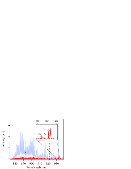
Figure 1: The full spectrum recorded at 4K showing the inhomogeneous line, with a zoom on the section of interest including two isolated quantum dots (X_a and X_b) and their respective bi-excitons (XX_a and XX_b), and the cavity mode (C).

To fabricate the samples, a layer of InAs self-assembled QDs is grown by molecular beam epitaxy and located at the center of a $\lambda$-GaAs microcavity surrounded by two planar Bragg mirrors, consisting of alternating layers of Al_0.1Ga_0.9As and Al_0.95Ga_0.05As. The top (bottom) mirror contains 28 (32) pairs of these layers. The quality factor of the planar cavity is 14000. In a subsequent step, the planar cavity is etched in order to form a micro-pillar containing the QDs. The specific micro-pillar discussed in the following has a diameter of 2.3 $\mu m$ and the density of the quantum dots is approximately $2.5\times 10^{-9}$ QDs/$\rm cm^{2}$.

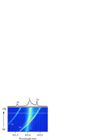
Figure 2: PL spectra of cavity and QD when varying the temperature (here from 5 K to 30 K). C indicates the cavity mode, whereas X_a and X_b corresponds to the two QDs spectrally closest to the cavity (see text). The white line indicates the temperature for which the spectrum shown in the top has been recorded.

The etching of the Bragg mirrors into a micro-pillar can deteriorate the quality factor of the cavity. To measure the micro-pillar quality factor, we perform a photoluminescence measurement at high power such that the ensemble of QDs act as a spectrally broad light source, which is used for probing the cavity Moreau01 ; Gayral . From this measurement, we extract a quality factor of our specific 2.3 $\mu m$ diameter sample mentioned above of $Q=\lambda/\Delta\lambda=7500$. This value agrees (to within 10%) with reflectivity measurement using white light. We will, in the following section, use the corresponding bare cavity linewidth $\kappa_{0}=\lambda/Q$ (in nanometers). Using equation 1 together with the measured value for the quality factor, we obtain $F_{P}=18.6$.

Our sample is located in a cryostat held at 4K. For the continuous-wave measurements, the QDs are excited using a standard laser diode emitting at 820 nm (off-resonant excitation in the GaAs barrier), while for the time resolved measurements, we use a pulsed Ti:Sa laser centered at 825 nm (80 MHz repetition rate and 1 ps pulse width). The emitted light is recollected after passing a spectrometer (1.5 m focal and 0.03 nm resolution). The spectrometer has two output channels: one channel leads to a CCD camera (for the CW measurements), the other to an avalanche photo diode (APD) with a 40 ps time resolution which, combined with a 5 ps resolution for the data acquisition card and 65 ps resolution due to the spectrometer, gives us an overall resolution of 80 ps.

In fig. 1 we give an overview of the different lines observed in a typical photoluminescence experiment for our particular micro-pillar to be studied in the following. Centered around 895 nm, we observe what is usually referred to as the inhomogeneous line, composed of hundreds of QDs. The micro-pillar has been processed such that the cavity resonance is located on the low energy wing of this inhomogeneous line, where the QD density is very low, allowing us to optically isolate one single QD (denoted $X_{a}$) to be studied, and in particular scanned through cavity resonance. We also note that its corresponding bi-exciton ($XX_{a}$) is blue shifted by about 1 nm, an amount which is larger than the cavity linewidth. For a given temperature, we can therefore make the bi-exciton off resonance with the cavity, while having the exciton centered at resonance. For this specific micro-pillar, this happens at 19.5 K. In this case, a second QD ($X_{b}$) appears about 3 cavity linewidths away (with its bi-exciton $XX_{b}$ even further away), and is therefore also minimally affected by the cavity. All other QDs are much further detuned.

In fig. 2 we show the temperature dependence of the cavity resonance frequency, as well as the two relevant QDs emission wavelengths. The cavity frequency varies due to a temperature dependent refractive index, while the QD exciton energy follows the expected temperature dependence of the GaAs bandgap. Due to this difference in temperature dependence, we can vary the cavity - QD detuning kiraz ; semicon ; Hennessy .

III Continuous-wave measurements

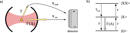
Figure 3: a) The PL of the QD arriving at the detector can be separated into two channels: one part emitted into loss channels ($\gamma$) but redirected to the detector with a probability $\chi_{leak}$ and the part emitted into the cavity $\Gamma(\Delta)$, and detected with a probability $\chi_{cav}$. b) Three-level scheme including the exciton $\mid X\rangle$ and bi-exciton $\mid XX\rangle$. The notations are defined in the text.

Even though the Purcell effect is a dynamical phenomenon, it can be measured without a time resolved setup. This can be understood as follows. As the emitter’s lifetime decreases near resonance due to the Purcell effect, it becomes harder to saturate the optical transition. This can be quantified by measuring the increase in the pump rate required to saturate the emitter (see section III.1), or by measuring the actual cycling rate in a PL measurement at saturation (section III.2). So by comparing the on- and off-resonant saturation pump rate or PL intensity, the Purcell-factor can be measured. More recently it has been demonstrated that one can also extract the Purcell-factor due to the change in the fraction of SE that is funneled into the cavity mode Gayral . This is done by measuring the SE rate as a function of detuning for fixed pump power, as will be done in section III.3.

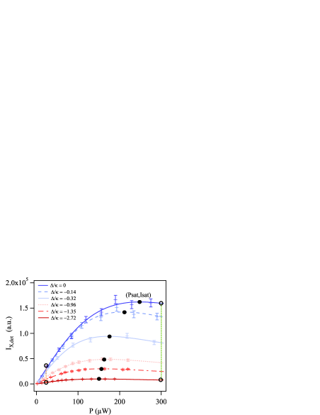
Figure 4: Photoluminescence intensity (I) as a function of pump power (P) for different cavity versus quantum dot detunings. The open circles allows us to extract $\epsilon_{above}$ and $\epsilon_{below}$ as described in section III.4. Filled black circles indicate the saturation intensity I_sat, and the corresponding pump power needed to saturate the QD, denoted P_sat.

An illustration of the principles is given in fig. 3. A QD is embedded in a cavity whose fundamental mode is nearly resonant with the excitonic $X_{a}$ transition (fig. 1a). We denote $\Delta$ the detuning between the excitonic transition and the cavity mode. The QD is non-resonantly pumped with a rate $r$, and decays by emitting photons either in the cavity mode, or in other leaky modes with a rate which we suppose to be independent of the detuning $\Delta$ and identical to that of the bulk material (which is a reasonable approximation for QDs in micro-pillar cavities Gerard98 and microdisks). As suggested by the PL spectra shown in part II, the QD should be modeled by a three-level system which includes the bi-exciton (fig. 3b). In the following we will concentrate solely on $X_{a}$, so for simplicity we will omit the subscript $a$. We denote $\gamma$ and $\gamma_{XX}$ the coupling of the X and bi-excitonic (XX) transition with the leaky modes. In addition to the leaky modes, the X transition is coupled to the cavity mode with a rate $\Gamma(\Delta)=\gamma F{\cal L}(\Delta)$ where $F$ is the effective Purcell factor experienced by the QD, taking into account that it is not perfectly coupled to the cavity (in contrast to $F_{P}$ given in equation 1, which is only an upper bound for $F$). Moreover, ${\cal L}(\Delta)=1/(1+\Delta^{2}/\kappa_{0}^{2})$ is a Lorentzian of width $\kappa_{0}$ corresponding to the empty cavity line shape. When pumping with a rate $r$, the average excitonic population is then given by

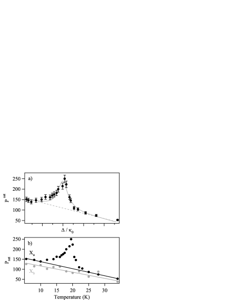
Figure 5: a) Saturation pump power as a function of detuning for our single QD and b) saturation pump power for our single QD $X_{a}$ and a “control” QD $X_{b}$ as a function of temperature. The QD $X_{a}$ goes through the cavity resonance while $X_{b}$ remains detuned throughout the scan.

$$p_{X}(\Delta,r)=\frac{1}{1+\frac{r}{\gamma_{XX}}+\frac{\gamma+\Gamma(\Delta)}{r}}.$$ (2)

As it was mentioned in the first part of this paper, the role of the cavity is not only to enhance the cycling rate for the exciton ($X$), but also to efficiently funnel the emitted photons into the cavity mode. Provided its emission pattern is directional, which is the case for micropillars, the coupling with a conveniently positioned detector can be very efficient, whereas the coupling between leaky modes and detector remains poor. These geometrical efficiencies are respectively denoted $\chi_{cav}$ and $\chi_{leak}$ (see fig. 3 and ref Auffeves ). The PL intensity from our single QD collected by the detector can thus be written in the following way:

$$I_{X,det}(\Delta,r)=I_{X}^{leak}(\Delta,r)+I_{X}^{cav}(\Delta,r),$$ (3)

where

$$I_{X}^{leak}(\Delta,r)=\chi_{leak}\gamma p_{X}(\Delta,r)$$ (4)

is the PL intensity emitted through the leaky modes and

$$I_{X}^{cav}(\Delta,r)=\chi_{cav}\Gamma(\Delta)p_{X}(\Delta,r)$$ (5)

the detected PL intensity emitted spatially into the cavity mode. Please note that the notation $cav$ applies to geometrical considerations, but not to the emission frequency (this PL contribution is indeed emitted at the QD frequency). In our experiment, to separate $I_{X,det}$ from the PL intensity from all other light sources, we use of the spectrometer to focus on a window centered on our selected QD (see the inset in fig. 1) and we then fit the line shape corresponding to the single QD with a Lorentzian function. When the QD-cavity detuning is large, it is easy to separate the QD line shape from the cavity, but as the detuning decreases, they will partially overlap with each other. When this happens, to avoid a part of the cavity peak erroneously being included in the single QD line shape, we also do a Lorentzian fit on the cavity profile, which we then subtract from the QD line shape. Note that in doing this, we also involuntarily omit from $I_{X,det}$ the part of the QD PL which is emitted at the cavity frequency, but this part constitutes a small fraction of the total signal.

An example of typical experimental data is pictured in fig. 4, where the PL intensities for different detunings $\Delta$ are plotted. As we generally measure the pump power denoted $P$ and not the pump rate $r$, we have chosen to plot the data as a function of the former (and we do the same in the graphs to follow). This also means that $P^{sat}$ is the pump power corresponding to the pump rate $r^{sat}$.

For each detuning, the maximal intensity $I_{X,det}^{sat}(\Delta,r^{sat}(\Delta))$ is reached when the X transition is saturated, where $r^{sat}(\Delta)$ denote the pump rate required to saturate the transition (saturation pump rate). Note that the highest values of $I_{X,det}^{sat}$ and corresponding $r^{sat}$ are reached at resonance, which is coherent with the enhancement of the X transition rate induced by the cavity. In the following, we will analyze the curves presented in fig. 4 (and further equivalent curves not added to the graph for clarity), in four different ways (section III.1-III.4).

III.1 Saturation pump rate measurements

In the first method the Purcell factor is extracted from the dependence of the saturating pumping rate intensity with the detuning $r^{sat}(\Delta)$, corresponding to black filled circles in fig. 4. This method has been proposed as a substitute for the time-resolved measurements, and has been widely used for micropillars bruno , microdiscs bruno and photonic crystals happ . The analytic expressions can be found by determining the pump rate corresponding to the maximum intensity of equation 3. We obtain

$$r^{sat}(\Delta)\propto\sqrt{1+F{\cal L}(\Delta)}.$$ (6)

In fig. 5a we have plotted the data and the fit according to equation 6 where we have imposed the bare cavity linewidth based on independent measurements. From the first fit, we extract a Purcell-factor of

$$F=3.7\pm 1.0,$$ (7)

where the relatively large error is due to the uncertainty of $r^{sat}$. The slope of the baseline in fig. 5a is due to the increase in temperature for increased detuning. As mentioned in section II, we use an optical excitation obtained through the pumping of the GaAs barrier material. The mean free path of the electrons and holes increase with temperature, so that the excitation rate of the QD tends to increase for a fixed pump rate. As a test, we have checked that the PL of another far detuned QD, $X_{b}$, gives rise to an equivalent slope during the same experiment, see fig. 5b.

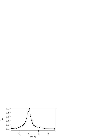
Figure 6: Saturation intensity for the single QD as a function of detuning. The size of the error-bars corresponds approximately to the extent of the data points and are therefore not shown.

III.2 Saturation PL intensity measurements

Another similar approach again based on the black filled circles in fig. 4 has been used in recent papers  Bockler ; pascale . This method corresponds to exploiting directly the maximum intensity of equation 3 given by

$$I_{X,det}^{sat}(\Delta)\propto\frac{F{\cal L}(\Delta)}{1+\sqrt{2+2F{\cal L}(\Delta)}},$$ (8)

In fig. 6 we have plotted the data and the fit (the maximum normalized to one) according to equation 8, again with the bare cavity linewidth fixed. From the fit, we extract a Purcell-factor of

$$F=2.4\pm 1.2.$$ (9)

In this case, the intrinsic uncertainty in the PL measurement is quite small, but is amplified by the fitting procedure, resulting in the stated errorbar.

III.3 PL intensity with fixed pump rate

In the two previous sections, we have used the data corresponding to the saturation pump rate and intensity. Instead, we can also use the emitted PL intensity, not at saturation, but for a fixed pump rate Gayral . This amounts to using the PL intensity corresponding to the intersection of the curves in fig. 4 with a straight vertical cut. In particular, we have plotted the PL intensity for powers below and above saturation in fig. 7. The fit corresponds again to equation 3, but this time with the pump rate fixed ($r=30\mu W$ and $r=300\mu W$, for the two curves, respectively). From both curves we have subtracted a global offset corresponding to the PL intensity $I_{X,det}$ at $\Delta=\infty$.

Below saturation the change in the light intensity $I_{X}^{cav}$ as the QD is scanned across the cavity resonance is due to the geometrical redirection of the emission alone (a modification in the emission pattern). What we detect is a projection of a fraction of the micro-pillar emission pattern onto the microscope aperture. More precisely, for low powers (well below saturation) $p_{X}(\Delta,r)=\frac{r}{\gamma+\Gamma(\Delta)}$, and we obtain

$$I_{X}^{cav}(\Delta)\propto\frac{F{\cal L}(\Delta)}{1+F{\cal L}(\Delta)}\equiv\beta(\Delta),$$ (10)

where we have defined the function $\beta(\Delta)$ which can be interpreted as the fraction of the emission pattern overlapping with the cavity mode. This function is broader than the Lorentzian profile of the cavity mode by a factor $\sqrt{(F+1)}$.

Above saturation, the geometrical redirection of the emission pattern is still present but the light intensity $I_{X}^{cav}$ follows now the ${\cal L}(\Delta)$ profile of the cavity owing to the additional effect of the larger emission rate of the quantum dot caused by the shortening of its lifetime. More precisely, in the regime well above saturation we have $p_{X}(\Delta,r)\approx\gamma_{XX}/r$, and we get

$$I_{X}^{cav}(\Delta,r)\propto F{\cal L}(\Delta).$$ (11)

From the ratio of the two widths, we extract a Purcell-factor of

$$F=3.2\pm 0.9,$$ (12)

where the stated uncertainty arises from the intensity measurements, which is the dominant source of error in this case.

III.4 PL intensity ratio at low and high pump rate

This method also consists in comparing the light emitted by the single QD at resonance and far from resonance, below and above saturation, but only requires four of the measurements used above. Here we do not subtract the offset due to $\chi_{leak}$ as done above, which has the advantage that it allows us to quantify $\chi_{cav}/\chi_{leak}$. We define as $\epsilon(\Delta,r)$ the following ratio

$$\epsilon(\Delta,r)=\frac{I_{X,det}(0,r)}{I_{X,det}(\Delta,r)}=\frac{p_{X}(0,r)}{p_{X}(\Delta,r)}\times\frac{\chi_{leak}+\chi_{cav}F}{\chi_{leak}+\chi_{cav}F{\cal L}(\Delta)}$$ (13)

$$\equiv\frac{p_{X}(0,r)}{p_{X}(\Delta,r)}\alpha(\Delta),$$ (14)

where the parameter $\alpha(\Delta)$ depends on the cavity funneling properties.

For pump rates below the pump rate required to saturate (where $p_{X}(\Delta,r)=\frac{r}{\gamma+\Gamma(\Delta)}$)

$$\epsilon_{below}(\Delta)=\alpha(\Delta)\times\frac{1+F{\cal L}(\Delta)}{1+F},$$ (15)

whereas above the saturation pump rate (again using that $p_{X}(\Delta,r)\approx\gamma_{XX}/r$)

$$\epsilon_{above}(\Delta)=\alpha(\Delta).$$ (16)

Taking the ratio between $\epsilon_{below}$ and $\epsilon_{above}$, $\alpha(\Delta)$ cancels, and with an independent measurement of $\kappa_{0}$ (see section II), we obtain a Purcell-Factor of

$$F=2.5\pm 0.5,$$ (17)

where the error arises from the uncertainty on the intensity measurements. From the separate value of $\epsilon_{above}$ (or $\epsilon_{below})$ we get

$$\chi_{cav}/\chi_{leak}\sim 15\pm 4.5,$$ (18)

confirming that the cavity is much better coupled to the detector than the leaky modes. This ratio depends on the radiation pattern of the micro-pillar, and the numerical aperture of the collection objective (0.4 for the above stated ratio of $\chi_{cav}/\chi_{leak}$).

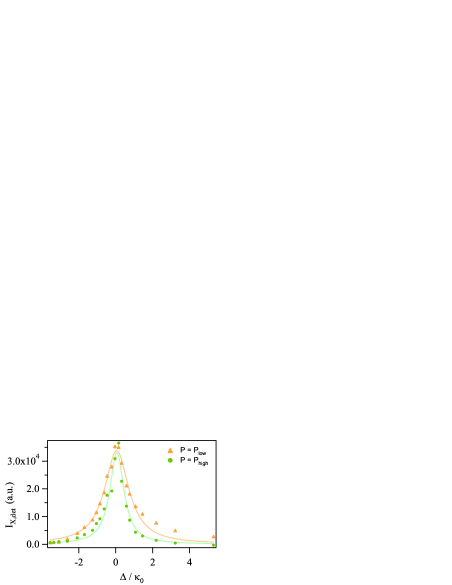
Figure 7: Measurements of the PL intensity at fixed pump power (30 $\mu W$ and 300 $\mu W$, respectively). The two curves can be thought of as the intersection of the curves in fig. 4 with vertical lines centered at P=30 $\mu W$ and P=300 $\mu W$ (with several more similar curves added).

Note that we have only included the presence of exciton and bi-exciton in all given formulas. We have, however, repeated the above analysis, allowing for all orders of exciton levels, without any significant change in final results within the range of used pump powers.

IV Time-resolved measurements

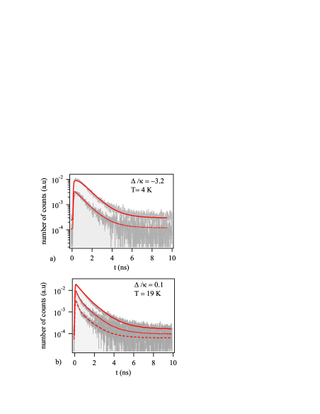
Figure 8: Lifetime measurements at different pump powers of the quantum dot while a) far detuned from the cavity and b) close to resonance. In a) the solid line corresponds to $P=3P_{sat}$ and dotted line to $P=P_{sat}$. In b) we have $P=P_{sat}$ (solid line) and $P=P_{sat}/10$ (dotted line) and $P=P_{sat}/30$ (dashed line).

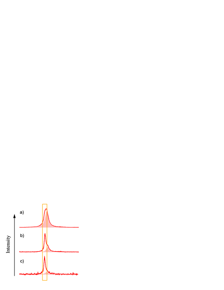
Figure 9: Three different line spectra, each corresponding to the QD (solid line) and the cavity (shaded area). The spectra are shown for the pump power decreasing from a) through c). For all three cases, the detuning is fixed ($\Delta=-0.2\kappa_{0}$). The square frame indicates for each spectrum the integration window.

As a way to confirm our continuous-wave measurements of the Purcell factor, we have performed a detailed study of the lifetime as a function of the detuning, using time resolved spectroscopy. This technique has been used extensively for many different systems since it was the first method to be used. In fact, the Purcell factor can be written as

$$F=\frac{\tau(\Delta=0)}{\tau(\Delta=\infty)}-1,$$ (19)

where $\tau$ is the lifetime of the QD, and $\Delta$ again is the detuning. Opposite equation 1, this definition also applies to an emitter that is not perfectly coupled to the cavity (within the approximation where $\gamma_{leak}=\gamma_{bulk}$, the latter denoting the SE of the QD into the unprocessed, or bulk, material).

In fig. 8 we show the measured lifetime of our quantum dot for different pumping powers. In a) the QD is detuned from the cavity resonance, while in b) it is at resonance. In the first case (a), we show two different powers. When $P\leq P_{sat}$ (lowest lying curve) the QD exhibits the typical mono-exponential decay. When $P\geq P_{sat}$ (highest lying curve), the effect of the bi-exciton can be observed as a rounding off of the curve at short time, which corresponds to the delay in the radiation of the exciton. The data fit very well with a model including three levels (a ground state, the exciton and bi-exciton states) and we extract the exciton and bi-exciton lifetimes, which are the same for the two different powers:

$$\tau_{X}=0.80\pm 0.05~{}{\rm ns}~{}~{}~{}{\rm and}~{}~{}~{}~{}\tau_{XX}=0.40\pm 0.02~{}{\rm ns}$$ (20)

As the biexciton is not influenced by the Purcell effect (for the detunings used in this experiment), the obtained value can be used as a fixed parameter when we then fit the data for the resonant case. Note that all our fits have been convoluted with the experimental system response time (80 ps time resolution). On the contrary, the resonant case (b), shows a power dependency that can not be explained by our simple three level model used above. We clearly observe in fig. 8b a change from a quasi mono-exponential decay to a bi-exponential decay, when lowering the pump rate. We exclude a prominent role of dark exciton since a mono-exponential behavior is observed in the non-resonant case (a). In addition, the fact that the second lifetime of the exponential decay is fast (less than 1 ns) also tends to eliminate this hypothesis. We believe that this behavior is due to detuned emitters, which contribute to the collected intensity via the cavity emission. Recent experiments Hennessy ; Englund ; Press ; Kaniber show that QD’s could emit photons in the cavity mode even at rather high detunings (several times the cavity linewidth). In contrast to CW measurements where we could separate the emission of our QD from the one of the cavity using appropriate lorentzian fits, in the present case we do not have access to the full spectra, and therefore cannot use the same technique. Instead we must select a frequency window around the QD line, for which we integrate all PL. This makes us unable to filter out the cavity component which overlaps in frequency with the chosen window (when close to resonance, as in fig. 8b). As a result we measure two different times: the shorter one is the lifetime of our single QD (undergoing Purcell effect), whereas the longer one corresponds to the lifetime of other detuned emitters. The higher the pump power, the more dominant is the signal due to the contribution of the detuned emitters. Therefore, at high powers, the light from other emitters tends to make the signal invisible for our single QD. This is illustrated in fig. 9, where we have shown the spectra corresponding to three different pump powers, ranging from high (a) to low (c), but for a fixed detuning. The fraction of light emitted via the cavity clearly dominates at high powers, but decrease while lowering the pump power.

This is why, for high powers, only one lifetime can be observed (upper curves in fig. 8b), and this lifetime is obviously no longer the QD radiative lifetime, but corresponds to the light emitted via the cavity. Only for lower pump power, the true lifetime also becomes visible (lower curve) as seen by the bi-exponential decay. We therefore need to include these additional emitters that we can model (within our pumping range) with a two-level system whose lifetime corresponds to an average lifetime, which can be measured in an independent experiment, in which all QDs are far detuned. We obtain $0.8\pm 0.05$ ns.

The exciton lifetime is the only free parameter in our fits (the bi-exciton lifetime is a fixed parameter). The excellent agreement between data and fit seems to validate our model. We find for the non resonant and resonant case, $\tau(\Delta=\infty)=0.80\pm 0.05$ ns and $\tau(\Delta=0)=0.2\pm 0.01$ ns, which gives a Purcell factor of:

$$F=3.0\pm 0.5$$ (21)

where the stated uncertainty arises from the exponential fit. Based on the above discussion, we remark that the low power condition is a necessary but not sufficient criterium for measuring the correct lifetime. Indeed, though all shown powers in fig. 8 are below saturation only the complete model gives the right lifetime. In fig. 10 we have plotted the exciton lifetime obtained by measurements equivalent to those in fig. 8 for different values of the detuning. The shape of the curve should be the Lorentzian profile of the cavity, confirmed by the fit.

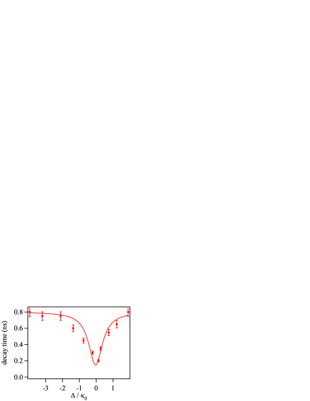
Figure 10: Exciton lifetimes measured at low intensity as a function of QD-cavity detuning.

V Final discussion

We have presented several ways to measure the Purcell-factor, which is an important figure of merit in cavity QED. All our CW measurements agree with each other, within the experimental uncertainty, for a Purcell-factor of $3.0\pm 0.4$. We emphasize that in our evaluation of the error-bars, we have not taken into account the stated 10 % uncertainty for the bare cavity linewidth (see section II). A simple PL measurement of the cavity linewidth has negligible error-bars, but when probing the cavity by reflectivity measurements, this value turns out to be about 10 % different. We also point out that the value measured by reflectivity is systematically higher than the one measured in PL. We will here revisit the obtained results for the Purcell factor, in order to see how a 10% deviation on the quality factor would affect the values. While the first method (based on saturation pump power, in section III.1) does not depend on this parameter, all the other CW methods here presented do. In particular, the second technique, which uses the saturation intensity (III.2), drastically depends on this parameter. In our case, an uncertainty of 10% on the quality factor would make the measurement based on this method useless. Though we still can fit the data with a correct shape, the obtained Purcell-factor is absurd and exceeds the theoretical value. Finally, concerning the third method (III.3), the modification of the Purcell factor induced by the 10% change in the quality factor amounts to 20 %, which is slightly below the stated error-bars due to the imprecision on the measurement. Therefore, these error-bars are not significantly increased when allowing the given deviation on the quality factor. The time resolved measurements also agree within the error-bars with the CW measurements. The fact that we clearly do not observe a single exponential decay at resonance, confirms the hypothesis that other light sources contribute to the light emitted into the cavity channel. In particular, for the time resolved measurement, if not including this light in our model, the lifetime appears to be pump power dependent, even when we pump way below saturation which is clearly non-physical. We thus underline that the commonly adopted criterium that the time resolved spectroscopy of an exciton has to be made below saturation, might not be sufficient for CQED experiment. Moreover, if additional emitters are present in the environment of the considered QD, it might be adequate to include their presence in the data analysis.

In conclusion, the agreement of the time resolved measurements with the CW measurements suggests that both methods are reliable. The dramatic influence of the cavity linewidth uncertainty on the Purcell-factor error-bars might be a reason for preferring Q-independent measurements such as time resolved spectroscopy. On the other hand, the time resolved measurements suffer from a lower signal-to-noise ratio, and for some systems (photonic crystals, in particular, where the radiation pattern is less favorable), this becomes a limiting factor, making the CW measurements more desirable. In that case, based on above considerations, we advise to use the method based on the saturation intensity with precaution, unless a very precise measurement of the cavity quality factor is available. If this is not the case, the other CW methods here presented seem more robust against an uncertainty on this parameter.

We thank B. Gayral for fruitful discussions and M. Rigault for his help and enthusiasm in the initial stages of the measurements, and we acknowledge QAP for financial support (Contract No. 15848).

References

- (1) M. Brune, F. Schmidt-Kaler, A. Maali, J. Dreyer, E. Hagley, J. M. Raimond, and S. Haroche, Phys. Rev. Lett. 76, 1800 (1996).
- (2) T. Puppe, I. Schuster, A. Grothe, A. Kubanek, K. Murr, P. W. H. Pinkse, and G. Rempe, Phys. Rev. Lett. 99, 013002 (2007), T. Wilk, S. C. Webster, A. Kuhn, and G. Rempe, Science 317, 488-490 (2007), T. Wilk, S. C. Webster, H. P. Specht, G. Rempe, and A. Kuhn, Phys. Rev. Lett. 98, 063601 (2007).
- (3) A. D. Boozer, A. Boca, R. Miller, T. E. Northup, and H. J. Kimble, Phys. Rev. Lett. 98, 193601 (2007).
- (4) A. A. Houck, D. I. Schuster, J. M. Gambetta, J. A. Schreier, B. R. Johnson, J. M. Chow, L. Frunzio, J. Majer, M. H. Devoret, S. M. Girvin, and R. J. Schoelkopf, Nature 449, 328-331 (2007).
- (5) J.M. Gérard, Top. Appl. Phys. 30, 269 (2003)
- (6) J. P. Reithmaier, G. Sek, A. Löffler, C. Hofmann, S. Kuhn, S. Reitzenstein, L. V. Keldysh, V. D. Kulakovskii, T. L. Reinecke, A. Forchel , Nature 432, 197 (2004); T. Yoshie, A. Scherer, J. Hendrickson, H. M. Gibbs, G. Rupper, C. Ell, O. B. Shchekin, D. G. Deppe, and G. Khitrova , Nature 432, 200 (2004); E. Peter, P. Senellart, D. Martrou, A. Lemaître, J. Hours, J. M. Gérard, and J. Bloch, Phys. Rev. Lett. 95, 067401 (2005).
- (7) K. Hennessy, A. Badolato, M. Winger, D. Gerace, M. Atatüre, S. Gulde, S. Fält, E. L. Hu and A. Imamoglu, Nature 445, 896 (2007).
- (8) D. Englund, A. Faraon, I. Fushman, N. Stoltz, P. Petroff, J. Vuckovic, Nature 450, 857-861 (2007).
- (9) M. T. Rakher, N. G. Stoltz, L. A. Coldren, P. M. Petroff, and D. Bouwmeester, Phys. Rev. Lett. 102, 097403 (2009)
- (10) D. Englund, A. Majumdar, A. Faraon, M. Toishi, N. Stoltz, P. Petroff, J. Vuckovic, arXiv: 0902.2428.
- (11) E. M. Purcell, Phys. Rev. 69, 681 (1946).
- (12) This requires that the emitter-cavity detuning is zero, that the emitter is located at the field antinode, that it is quasi-monochromatic (linewidth much smaller than the cavity linewidth), and that the polarisation is the same as that of the cavity mode.
- (13) J. M. Gérard, B. Sermage, B. Gayral, B. Legrand, E. Costard, and V. Thierry-Mieg, Phys. Rev. Lett. 81, 1110 (1998)
- (14) G. S. Solomon, M. Pelton, and Y. Yamamoto, Phys. Rev. Lett. 86, 3903 (2001).
- (15) E. Moreau, I. Robert, J. M. Gérard, I. Abram, L. Manin, and V. Thierry-Mieg, Applied Physics Letters 79, 2865 (2001).
- (16) D. Press, S. G tzinger, S. Reitzenstein, C. Hofmann, A. Löffler, M. Kamp, A. Forchel, and Y. Yamamoto Phys. Rev. Lett. 98, 117402 (2007).
- (17) Charles Santori, David Fattal, Jelena Vuckovic, Glenn S. Solomon and Yoshihisa Yamamoto, Nature 419, 594 (2002)
- (18) S. Varoutsis, S. Laurent, P. Kramper, A. Lemaître, I. Sagnes, I. Robert-Philip, and I. Abram, Phys. Rev. B 72, 041303(R), (2005)
- (19) A. Auffèves-Garnier, C. Simon, J.-M. Gérard, and J.-P. Poizat, Phys. Rev. A 75, 053823 (2007).
- (20) J.M. Gérard and B. Gayral, J Lightwave Technol. 17, 2089 (1999)
- (21) M. Kaniber, A. Laucht, A. Neumann, J. M. Villas-Bôas, M. Bichler, M.-C. Amann, and J. J. Finley, Phys. Rev. B 77, 161303(R) (2008).
- (22) A. Naesby, T. Suhr, P. T. Kristensen, and J. Mørk, Phys. Rev. A 78, 045802 (2008).
- (23) M. Yamaguchi, T. Asano, S. Noda, Optics Express 16,18067 (2008).
- (24) A. Auff ves, J.-M. Gérard, and J.-P. Poizat Phys. Rev. A 79, 053838 (2009)
- (25) B. Gayral and J.M. Gérard, Phys. Rev. B 78, 235306 (2008).
- (26) A. Kiraz, P. Michler, C. Becher, B. Gayral, A. Imamoglu, L. Zhang, E. Hu, Appl. Phys. Lett. 78, 3932 (2001)
- (27) T. D. Happ, I. Tartakovskii, V.D. Kulakovslii, J. P. Reithmaier, M. Kamp, A. Forchel, Phys. Rev. B 66, R041303 (2002)
- (28) C. Böckler et al. Applied Physics Letters, 92, 091107 (2008).
- (29) A. Dousse, L. Lanco, J. Suffczyn’ski, E. Semenova, A. Miard, A. Lemaître, I. Sagnes, C. Roblin, J. Bloch, and P. Senellart, Phys. Rev. Lett. 101, 267404 (2008).