Positivity for cluster algebras from surfaces

Abstract.

We give combinatorial formulas for the Laurent expansion of any cluster variable in any cluster algebra coming from a triangulated surface (with or without punctures), with respect to an arbitrary seed. Moreover, we work in the generality of principal coefficients. An immediate corollary of our formulas is a proof of the positivity conjecture of Fomin and Zelevinsky for cluster algebras from surfaces, in geometric type.

1. Introduction

Since their introduction by Fomin and Zelevinsky in [FZ1], cluster algebras have been shown to be related to diverse areas of mathematics such as total positivity, quiver representations, Teichmüller theory, tropical geometry, Lie theory, and Poisson geometry. One of the main outstanding conjectures about cluster algebras is the positivity conjecture, which says that if one fixes a cluster algebra $\mathcal{A}$ and an arbitrary cluster $\mathbf{x}$, one can express each cluster variable $x\in\mathcal{A}$ as a Laurent polynomial with positive coefficients in the variables of $\mathbf{x}$.

There is a class of cluster algebras arising from surfaces with marked points, introduced by Fomin, Shapiro, and Thurston in [FST] (generalizing work of Fock and Goncharov [FG1, FG2] and Gekhtman, Shapiro, and Vainshtein [GSV]), and further developed in [FT]. This class is quite large: (assuming rank at least three) it has been shown [FeShTu] that all but finitely many skew-symmetric cluster algebras of finite mutation type come from this construction. Note that the class of cluster algebras of finite mutation type in particular contains those of finite type.

The goal of this paper is to give a combinatorial expression for the Laurent polynomial which expresses any cluster variable in terms of any cluster, for any cluster algebra arising from a surface. An immediate corollary is the proof of the positivity conjecture for all cluster algebras arising from surfaces.

A cluster algebra $\mathcal{A}$ of rank $n$ is a subalgebra of an ambient field $\mathcal{F}$ isomorphic to a field of rational functions in $n$ variables. Each cluster algebra has a distinguished set of generators called cluster variables; this set is a union of overlapping algebraically independent $n$-subsets of $\mathcal{F}$ called clusters, which together have the structure of a simplicial complex called the cluster complex. See Definition 2.5 for precise details. The clusters are related to each other by birational transformations of the following kind: for every cluster $\mathbf{x}$ and every cluster variable $x\in\mathbf{x}$, there is another cluster $\mathbf{x}^{\prime}=\mathbf{x}-\{x\}\cup\{x^{\prime}\}$, with the new cluster variable $x^{\prime}$ determined by an exchange relation of the form

$$xx^{\prime}=y^{+}M^{+}+y^{-}M^{-}.$$

Here $y^{+}$ and $y^{-}$ belong to a coefficient semifield $\mathbb{P}$, while $M^{+}$ and $M^{-}$ are two monomials in the elements of $\mathbf{x}-\{x\}$. There are two dynamics at play in the exchange relations: that of the monomials $M^{+}$ and $M^{-}$, which is encoded in the exchange matrix, and that of the coefficients.

A classification of finite type cluster algebras – those with finitely many clusters – was given by Fomin and Zelevinksy in [FZ2]. They showed that this classification is parallel to the famous Cartan-Killing classification of complex simple Lie algebras, i.e. finite type cluster algebras either fall into one of the infinite families $A_{n}$, $B_{n}$, $C_{n}$, $D_{n}$, or are of one of the exceptional types $E_{6},E_{7},E_{8},F_{4}$, or $G_{2}$. Furthermore, the type of a finite type cluster algebra depends only on the dynamics of the corresponding exchange matrices, and not on the coefficients. However, there are many examples of cluster algebras of geometric origin which – despite having the same type – have totally different systems of coefficients. This motivated Fomin and Zelevinsky’s work in [FZ4], in which they studied the dependence of a cluster algebra structure on the choice of coefficients. One surprising result of [FZ4] was that there is a special choice of coefficients, the principal coefficients, which have the property that computation of explicit expansion formulas for the cluster variables in arbitrary cluster algebras can be reduced to computation of explicit expansion formulas in cluster algebras with principal coefficients. A corollary of this work is that to prove the positivity conjecture in geometric type, it suffices to prove the positivity conjecture for the class of principal coefficients.

This takes us to the topic of the present work. Our main results are combinatorial formulas for cluster expansions of cluster variables with respect to any seed, in any cluster algebra coming from a surface. Our formulas are manifestly positive, so as a consequence we obtain the following result.

Theorem 1.1.

Let $\mathcal{A}$ be any cluster algebra arising from a surface, where the coefficient system is of geometric type, and let $\mathbf{x}$ be any choice of initial cluster. Then the Laurent expansion of every cluster variable with respect to the cluster $\mathbf{x}$ has non-negative coefficients.

Our results generalize those obtained in [S2], where cluster algebras from the (much more restrictive) case of surfaces without punctures were considered. This work in turn generalized [ST], which treated cluster algebras from unpunctured surfaces with a very limited coefficient system that was associated to the boundary of the surface. The very special case where the surface is a polygon and coefficients arise from the boundary was covered in [S], and also in unpublished work [CP, FZ3]. See also [Pr2]. The recent paper [MS] gave an alternative formulation of the results of [S2], using the language of perfect matchings as opposed to $T$-paths.

Many other people have worked on the problem of finding Laurent expansions of cluster variables, and on the positivity conjecture. However, most of the results so far obtained have strong restrictions on the cluster algebra, the choice of initial cluster (equivalently, initial seed), or on the system of coefficients.

In the case of rank 2 cluster algebras, the papers [SZ, Z, MP] gave cluster expansion formulas in affine types. Positivity in these cases was subsequently generalized to the coefficient-free rank 2 case in [Dup], using results of [CR]. In the case of finite type cluster algebras, the positivity conjecture with respect to a bipartite seed follows from [FZ4, Corollary 11.7]. Other work [M] gave cluster expansions for coefficient-free cluster algebras of finite classical types with respect to a bipartite seed.

A recent tool in understanding Laurent expansions of cluster variables is the connection to quiver representations and the introduction of the cluster category [BMRRT] (see also [CCS1] in type $A$). More specifically, there is a geometric interpretation (found in [CC] and generalized in [CK]) of coefficients in Laurent expansions as Euler-Poincaré characteristics of appropriate Grassmannians of quiver representations. Using this approach, the works [CC, CK, CK2] gave an expansion formula in the case where the cluster algebra is acyclic and the initial cluster lies in an acyclic seed (see also [CZ] in rank 2); this was subsequenty generalized to arbitrary clusters in an acyclic cluster algebra [Pa]. Note that these formulas do not give information about the coefficients. Later, [FK] generalized these results to cluster algebras with principal coefficients that admit a categorification by a 2-Calabi-Yau category [FK]; by [A] and [ABCP, LF], such a categorification exists in the case of cluster algebras associated to surfaces with non-empty boundary. Recently [DWZ] gave expressions for the $F$-polynomials in any skew-symmetric cluster algebra. However, since all of the above formulas are in terms of Euler-Poincaré characteristics (which can be negative), they do not immediately imply the positivity conjecture.

The work [CR] used the above approach to prove the positivity conjecture for coefficient-free acyclic cluster algebras, with respect to an acyclic seed. Building on results of [HL], Nakajima recently used quiver varieties to prove the positivity conjecture for cluster algebras that have at least one bipartite seed, with respect to any cluster [N]. This is a very strong result, but it does not overlap very much with our Theorem 1.1. Note that a bipartite seed is in particular acyclic, but not every acyclic type has a bipartite seed; the affine type $\tilde{A}_{2}$, for example, does not. And the only surfaces that give rise to acyclic cluster algebras are the polygon, the polygon with one puncture, the annulus, and the polygon with two punctures (corresponding to the finite types $A$ and $D$, and the affine types $\tilde{A}$ and $\tilde{D}$). All other surfaces yield non-acyclic cluster algebras, see [FST, Corollary 12.4].

The paper is organized as follows. We give background on cluster algebras and cluster algebras from surfaces in Sections 2 and 3. In Section 4 we present our formulas for Laurent expansions of cluster variables, and in Section 5 we give examples, as well as identities in the coefficient-free case. As the proofs of our main results are rather involved, we give a detailed outline of the main argument in Section 6, before giving the proofs themselves in Sections 7 to 10 and 12. In Section 13, we combine our results with those of [FK] and [DWZ] to give formulas for F-polynomials, g-vectors, and Euler-Poincaré characteristics of quiver Grassmannians.

Recall that cluster variables in cluster algebras from surfaces correspond to ordinary arcs as well as arcs with notches at one or two ends. We remark that working in the generality of principal coefficients is much more difficult than working in the coefficient-free case. Indeed, once we have proved positivity for cluster variables corresponding to ordinary arcs, the proof of positivity for cluster variables corresponding to tagged arcs in the coefficient-free case follows easily, see Proposition 5.3 and Section 11. Putting back principal coefficients requires much more elaborate arguments, see Section 12. A crucial tool here is the connection to laminations [FT].

Note that all cluster algebras coming from surfaces are skew-symmetric. In a sequel to this paper we will explain how to use folding arguments to give positivity results for cluster algebras with principal coefficients which are not skew-symmetric.

Acknowledgements: We are grateful to the organizers of the workshop on cluster algebras in Morelia, Mexico, where we benefited from Dylan Thurston’s lectures. We would also like to thank Sergey Fomin and Bernard Leclerc for useful discussions.

2. Cluster algebras

We begin by reviewing the definition of cluster algebra, first introduced by Fomin and Zelevinsky in [FZ1]. Our definition follows the exposition in [FZ4].

2.1. What is a cluster algebra?

To define a cluster algebra $\mathcal{A}$ we must first fix its ground ring. Let $(\mathbb{P},\oplus,\cdot)$ be a semifield, i.e., an abelian multiplicative group endowed with a binary operation of (auxiliary) addition $\oplus$ which is commutative, associative, and distributive with respect to the multiplication in $\mathbb{P}$. The group ring $\mathbb{Z}\mathbb{P}$ will be used as a ground ring for $\mathcal{A}$. One important choice for $\mathbb{P}$ is the tropical semifield; in this case we say that the corresponding cluster algebra is of geometric type.

Definition 2.1 (Tropical semifield).

Let $\operatorname{Trop}(u_{1},\dots,u_{m})$ be an abelian group (written multiplicatively) freely generated by the $u_{j}$. We define $\oplus$ in $\operatorname{Trop}(u_{1},\dots,u_{m})$ by

(2.1) $$\prod_{j}u_{j}^{a_{j}}\oplus\prod_{j}u_{j}^{b_{j}}=\prod_{j}u_{j}^{\min(a_{j},b_{j})}\,,$$

and call $(\operatorname{Trop}(u_{1},\dots,u_{m}),\oplus,\cdot)$ a tropical semifield. Note that the group ring of $\operatorname{Trop}(u_{1},\dots,u_{m})$ is the ring of Laurent polynomials in the variables $u_{j}\,$.

As an ambient field for $\mathcal{A}$, we take a field $\mathcal{F}$ isomorphic to the field of rational functions in $n$ independent variables (here $n$ is the rank of $\mathcal{A}$), with coefficients in $\mathbb{Q}\mathbb{P}$. Note that the definition of $\mathcal{F}$ does not involve the auxiliary addition in $\mathbb{P}$.

Definition 2.2 (Labeled seeds).

A labeled seed in $\mathcal{F}$ is a triple $(\mathbf{x},\mathbf{y},B)$, where

• $\mathbf{x}=(x_{1},\dots,x_{n})$ is an $n$-tuple of elements of $\mathcal{F}$ forming a free generating set over $\mathbb{Q}\mathbb{P}$,

• $\mathbf{y}=(y_{1},\dots,y_{n})$ is an $n$-tuple of elements of $\mathbb{P}$, and

• $B=(b_{ij})$ is an $n\!\times\!n$ integer matrix which is skew-symmetrizable.

That is, $x_{1},\dots,x_{n}$ are algebraically independent over $\mathbb{Q}\mathbb{P}$, and $\mathcal{F}=\mathbb{Q}\mathbb{P}(x_{1},\dots,x_{n})$. We refer to $\mathbf{x}$ as the (labeled) cluster of a labeled seed $(\mathbf{x},\mathbf{y},B)$, to the tuple $\mathbf{y}$ as the coefficient tuple, and to the matrix $B$ as the exchange matrix.

We obtain (unlabeled) seeds from labeled seeds by identifying labeled seeds that differ from each other by simultaneous permutations of the components in $\mathbf{x}$ and $\mathbf{y}$, and of the rows and columns of $B$.

We use the notation $[x]_{+}=\max(x,0)$, $[1,n]=\{1,\dots,n\}$, and

$$\operatorname{sgn}(x) =\begin{cases}-1&\text{if $x<0$;}\\ 0&\text{if $x=0$;}\\ 1&\text{if $x>0$.}\end{cases}$$

Definition 2.3 (Seed mutations).

Let $(\mathbf{x},\mathbf{y},B)$ be a labeled seed in $\mathcal{F}$, and let $k\in[1,n]$. The seed mutation $\mu_{k}$ in direction $k$ transforms $(\mathbf{x},\mathbf{y},B)$ into the labeled seed $\mu_{k}(\mathbf{x},\mathbf{y},B)=(\mathbf{x}^{\prime},\mathbf{y}^{\prime},B^{\prime})$ defined as follows:

• The entries of $B^{\prime}=(b^{\prime}_{ij})$ are given by

  (2.2) $$b^{\prime}_{ij}=\begin{cases}-b_{ij}&\text{if $i=k$ or $j=k$;}\\[3.61371pt] b_{ij}+\operatorname{sgn}(b_{ik})\ [b_{ik}b_{kj}]_{+}&\text{otherwise.}\end{cases}$$

• The coefficient tuple $\mathbf{y}^{\prime}=(y_{1}^{\prime},\dots,y_{n}^{\prime})$ is given by

  (2.3) $$y^{\prime}_{j}=\begin{cases}y_{k}^{-1}&\text{if $j=k$};\\[3.61371pt] y_{j}y_{k}^{[b_{kj}]_{+}}(y_{k}\oplus 1)^{-b_{kj}}&\text{if $j\neq k$}.\end{cases}$$

• The cluster $\mathbf{x}^{\prime}=(x_{1}^{\prime},\dots,x_{n}^{\prime})$ is given by $x_{j}^{\prime}=x_{j}$ for $j\neq k$, whereas $x^{\prime}_{k}\in\mathcal{F}$ is determined by the exchange relation

  (2.4) $$x^{\prime}_{k}=\frac{y_{k}\ \prod x_{i}^{[b_{ik}]_{+}}+\ \prod x_{i}^{[-b_{ik}]_{+}}}{(y_{k}\oplus 1)x_{k}}\,.$$

We say that two exchange matrices $B$ and $B^{\prime}$ are mutation-equivalent if one can get from $B$ to $B^{\prime}$ by a sequence of mutations.

Definition 2.4 (Patterns).

Consider the $n$-regular tree $\mathbb{T}_{n}$ whose edges are labeled by the numbers $1,\dots,n$, so that the $n$ edges emanating from each vertex receive different labels. A cluster pattern is an assignment of a labeled seed $\Sigma_{t}=(\mathbf{x}_{t},\mathbf{y}_{t},B_{t})$ to every vertex $t\in\mathbb{T}_{n}$, such that the seeds assigned to the endpoints of any edge $t\!\begin{array}[]{c}\scriptstyle{k}\\[-7.22743pt] -\!\!\!-\!\!\!-\\[-7.22743pt] {}\scriptstyle\hfil\end{array}\!t^{\prime}$ are obtained from each other by the seed mutation in direction $k$. The components of $\Sigma_{t}$ are written as:

(2.5) $$\mathbf{x}_{t}=(x_{1;t}\,,\dots,x_{n;t})\,,\quad\mathbf{y}_{t}=(y_{1;t}\,,\dots,y_{n;t})\,,\quad B_{t}=(b^{t}_{ij})\,.$$

Clearly, a cluster pattern is uniquely determined by an arbitrary seed.

Definition 2.5 (Cluster algebra).

Given a cluster pattern, we denote

(2.6) $$\mathcal{X}=\bigcup_{t\in\mathbb{T}_{n}}\mathbf{x}_{t}=\{x_{i,t}\,:\,t\in\mathbb{T}_{n}\,,\ 1\leq i\leq n\}\ ,$$

the union of clusters of all the seeds in the pattern. The elements $x_{i,t}\in\mathcal{X}$ are called cluster variables. The cluster algebra $\mathcal{A}$ associated with a given pattern is the $\mathbb{Z}\mathbb{P}$-subalgebra of the ambient field $\mathcal{F}$ generated by all cluster variables: $\mathcal{A}=\mathbb{Z}\mathbb{P}[\mathcal{X}]$. We denote $\mathcal{A}=\mathcal{A}(\mathbf{x},\mathbf{y},B)$, where $(\mathbf{x},\mathbf{y},B)$ is any seed in the underlying cluster pattern.

The remarkable Laurent phenomenon asserts the following.

Theorem 2.6.

[FZ1, Theorem 3.1] The cluster algebra $\mathcal{A}$ associated with a seed $(\mathbf{x},\mathbf{y},B)$ is contained in the Laurent polynomial ring $\mathbb{Z}\mathbb{P}[\mathbf{x}^{\pm 1}]$, i.e. every element of $\mathcal{A}$ is a Laurent polynomial over $\mathbb{Z}\mathbb{P}$ in the cluster variables from $\mathbf{x}=(x_{1},\dots,x_{n})$.

Definition 2.7.

Let $\mathcal{A}$ be a cluster algebra, $\Sigma$ be a seed, and $x$ be a cluster variable of $\mathcal{A}$. We denote by $[x]_{\Sigma}^{\mathcal{A}}$ the Laurent polynomial given by Theorem 2.6 which expresses $x$ in terms of the cluster variables from $\Sigma$. We refer to this as the cluster expansion of $x$ in terms of $\Sigma$.

The longstanding positivity conjecture [FZ1] says that even more is true.

Conjecture 2.8.

(Positivity Conjecture) For any cluster algebra $\mathcal{A}$, any seed $\Sigma$, and any cluster variable $x$, the Laurent polynomial $[x]_{\Sigma}^{\mathcal{A}}$ has coefficients which are non-negative integer linear combinations of elements in $\mathbb{P}$.

Remark 2.9.

In cluster algebras whose ground ring is $\operatorname{Trop}(u_{1},\dots,u_{m})$ (the tropical semifield), it is convenient to replace the matrix $B$ by an $(n+m)\times n$ matrix $\tilde{B}=(b_{ij})$ whose upper part is the $n\times n$ matrix $B$ and whose lower part is an $m\times n$ matrix that encodes the coefficient tuple via

(2.7) $$y_{k}=\prod_{i=1}^{m}u_{i}^{b_{(n+i)k}}.$$

Then the mutation of the coefficient tuple in equation (2.3) is determined by the mutation of the matrix $\tilde{B}$ in equation (2.2) and the formula (2.7); and the exchange relation (2.4) becomes

(2.8) $$x_{k}^{\prime}=x_{k}^{-1}\left(\prod_{i=1}^{n}x_{i}^{[b_{ik}]_{+}}\prod_{i=1}^{m}u_{i}^{[b_{(n+i)k}]_{+}}+\prod_{i=1}^{n}x_{i}^{[-b_{ik}]_{+}}\prod_{i=1}^{m}u_{i}^{[-b_{(n+i)k}]_{+}}\right).$$

2.2. Finite type and finite mutation type classification

We say that a cluster algebra is of finite type if it has finitely many seeds. Fomin and Zelevinsky [FZ2] showed that the classification of finite type cluster algebras is parallel to the Cartan-Killing classification of complex simple Lie algebras.

More specifically, define the diagram $\Gamma(B)$ associated to an $n\times n$ exchange matrix $B$ to be a weighted directed graph on $n$ nodes $v_{1},\dots,v_{n}$, where $v_{i}$ is directed towards $v_{j}$ if and only if $b_{ij}>0$. In that case, we label this edge by the weight $|b_{ij}b_{ji}|.$ It was shown in [FZ2] that a cluster algebra $\mathcal{A}=\mathcal{A}(\mathbf{x},\mathbf{y},B)$ is of finite type if and only $\Gamma(B)$ is mutation-equivalent to an orientation of a finite type Dynkin diagram. In this case, we say that $B$ and $\Gamma(B)$ are of finite type.

We say that a matrix $B$ (and the corresponding cluster algebra) has finite mutation type if its mutation equivalence class is finite, i.e. only finitely many matrices can be obtained from $B$ by repeated matrix mutations. A classification of all cluster algebras of finite mutation type with skew-symmetric exchange matrices was recently given by Felikson, Shapiro, and Tumarkin [FeShTu]. In particular, all but 11 of them come from either cluster algebras of rank 2 or cluster algebras associated with triangulations of surfaces (see Section 3).

2.3. Cluster algebras with principal coefficients

Fomin and Zelevinsky introduced in [FZ4] a special type of coefficients, called principal coefficients.

Definition 2.10 (Principal coefficients).

We say that a cluster pattern $t\mapsto(\mathbf{x}_{t},\mathbf{y}_{t},B_{t})$ on $\mathbb{T}_{n}$ (or the corresponding cluster algebra $\mathcal{A}$) has principal coefficients at a vertex $t_{0}$ if $\mathbb{P}=\operatorname{Trop}(y_{1},\dots,y_{n})$ and $\mathbf{y}_{t_{0}}=(y_{1},\dots,y_{n})$. In this case, we denote $\mathcal{A}=\mathcal{A}_{\bullet}(B_{t_{0}})$.

Remark 2.11.

Definition 2.10 can be rephrased as follows: a cluster algebra $\mathcal{A}$ has principal coefficients at a vertex $t_{0}$ if $\mathcal{A}$ is of geometric type, and is associated with the matrix $\tilde{B}_{t_{0}}$ of order $2n\times n$ whose upper part is $B_{t_{0}}$, and whose complementary (i.e., bottom) part is the $n\times n$ identity matrix (cf. [FZ1, Corollary 5.9]).

Definition 2.12 (The functions $X_{\ell;t}$ and $F_{\ell,t}$).

Let $\mathcal{A}$ be the cluster algebra with principal coefficients at $t_{0}$, defined by the initial seed $\Sigma_{t_{0}}=(\mathbf{x}_{t_{0}}\,,\mathbf{y}_{t_{0}}\,,B_{t_{0}})$ with

(2.9) $$\mathbf{x}_{t_{0}}=(x_{1},\dots,x_{n}),\quad\mathbf{y}_{t_{0}}=(y_{1},\dots,y_{n}),\quad B_{t_{0}}=B^{0}=(b^{0}_{ij})\,.$$

By the Laurent phenomenon, we can express every cluster variable $x_{\ell;t}$ as a (unique) Laurent polynomial in $x_{1},\dots,x_{n},y_{1},\dots,y_{n}$; we denote this by

(2.10) $$X_{\ell;t}=X_{\ell;t}^{B^{0};t_{0}}.$$

Let $F_{\ell;t}=F_{\ell;t}^{B^{0};t_{0}}$ denote the Laurent polynomial obtained from $X_{\ell;t}$ by

(2.11) $$F_{\ell;t}(y_{1},\dots,y_{n})=X_{\ell;t}(1,\dots,1;y_{1},\dots,y_{n}).$$

$F_{\ell;t}(y_{1},\dots,y_{n})$ turns out to be a polynomial [FZ4] and is called an F-polynomial.

Knowing the cluster expansions for a cluster algebra with principal coefficients allows one to compute the cluster expansions for the “same” cluster algebra with an arbitrary coefficient system. To explain this, we need an additional notation. If $F$ is a subtraction-free rational expression over $\mathbb{Q}$ in several variables, $R$ a semifield, and $u_{1},\dots,u_{r}$ some elements of $R$, then we denote by $F|_{R}(u_{1},\dots,u_{r})$ the evaluation of $F$ at $u_{1},\dots,u_{r}\,$.

Theorem 2.13.

[FZ4, Theorem 3.7] Let $\mathcal{A}$ be a cluster algebra over an arbitrary semifield $\mathbb{P}$ and contained in the ambient field $\mathcal{F}$, with a seed at an initial vertex $t_{0}$ given by

$$((x_{1},\dots,x_{n}),(y_{1}^{*},\dots,y_{n}^{*}),B^{0}).$$

Then the cluster variables in $\mathcal{A}$ can be expressed as follows:

(2.12) $$x_{\ell;t}=\frac{X_{\ell;t}^{B^{0};t_{0}}|_{\mathcal{F}}(x_{1},\dots,x_{n};y_{1}^{*},\dots,y_{n}^{*})}{F_{\ell;t}^{B^{0};t_{0}}|_{\mathbb{P}}(y_{1}^{*},\dots,y_{n}^{*})}\,.$$

When $\mathbb{P}$ is a tropical semifield, the denominator of equation (2.12) is a monomial. Therefore if the Laurent polynomial $X_{\ell;t}$ has positive coefficients, so does $x_{\ell;t}$.

Corollary 2.14.

Let $\mathcal{A}$ be the cluster algebra with principal coefficients at a vertex $t_{0}$, defined by the initial seed $\Sigma_{t_{0}}=(\mathbf{x}_{t_{0}}\,,\mathbf{y}_{t_{0}}\,,B_{t_{0}})$. Let $\hat{\mathcal{A}}$ be any cluster algebra of geometric type defined by the same exchange matrix $B_{t_{0}}$. If the positivity conjecture holds for $\mathcal{A}$, then it also holds for $\hat{\mathcal{A}}$.

3. Cluster algebras arising from surfaces

Building on work of Fock and Goncharov [FG1, FG2], and of Gekhtman, Shapiro and Vainshtein [GSV], Fomin, Shapiro and Thurston [FST] associated a cluster algebra to any bordered surface with marked points. In this section we will recall that construction, as well as further results of Fomin and Thurston [FT].

Definition 3.1 (Bordered surface with marked points).

Let $S$ be a connected oriented 2-dimensional Riemann surface with (possibly empty) boundary. Fix a nonempty set $M$ of marked points in the closure of $S$ with at least one marked point on each boundary component. The pair $(S,M)$ is called a bordered surface with marked points. Marked points in the interior of $S$ are called punctures.

Table 1 gives examples of surfaces (using notation of Lemma 3.5). For technical reasons, we require that $(S,M)$ is not a sphere with one, two or three punctures; a monogon with zero or one puncture; or a bigon or triangle without punctures.

b	g	c	p	n	surface
0	1	0	1	3	punctured torus
0	0	0	4	6	sphere with 4 punctures
1	0	n+3	0	c-3	polygon
1	0	n	1	c	once punctured polygon
1	0	n-3	2	c+3	twice punctured polygon
1	1	n-3	0	c+3	torus with disk removed
2	0	n	0	c	annulus
2	0	n-3	1	c+3	punctured annulus
2	1	n-6	0	c+6	torus with 2 disks removed
3	0	n-3	0	c+3	pair of pants

Table 1. Examples of surfaces

3.1. Ideal triangulations and tagged triangulations

Definition 3.2 (Ordinary arcs).

An arc $\gamma$ in $(S,M)$ is a curve in $S$, considered up to isotopy, such that

• the endpoints of $\gamma$ are in $M$;

• $\gamma$ does not cross itself, except that its endpoints may coincide;

• except for the endpoints, $\gamma$ is disjoint from $M$ and from the boundary of $S$,

• $\gamma$ does not cut out an unpunctured monogon or an unpunctured bigon.

An arc whose endpoints coincide is called a loop. Curves that connect two marked points and lie entirely on the boundary of $S$ without passing through a third marked point are boundary segments. By (c), boundary segments are not ordinary arcs.

Definition 3.3 (Crossing numbers and compatibility of ordinary arcs).

For any two arcs $\gamma,\gamma^{\prime}$ in $S$, let $e(\gamma,\gamma^{\prime})$ be the minimal number of crossings of arcs $\alpha$ and $\alpha^{\prime}$, where $\alpha$ and $\alpha^{\prime}$ range over all arcs isotopic to $\gamma$ and $\gamma^{\prime}$, respectively. We say that arcs $\gamma$ and $\gamma^{\prime}$ are compatible if $e(\gamma,\gamma^{\prime})=0$.

Definition 3.4 (Ideal triangulations).

An ideal triangulation is a maximal collection of pairwise compatible arcs (together with all boundary segments). The arcs of a triangulation cut the surface into ideal triangles.

Lemma 3.5.

[FG3, Section 2] Each ideal triangulation consists of $n=6g+3b+3p+c-6$ arcs, where $g$ is the genus of $S$, $b$ is the number of boundary components, $p$ is the number of punctures and $c=|M|-p$ is the number of marked points on the boundary of $S$. The number $n$ is called the rank of $(S,M)$. The number of triangles in any triangulation is $4g+2b+2p+c-4.$

There are two types of ideal triangles: triangles that have three distinct sides and triangles that have only two. The latter are called self-folded triangles. Note that a self-folded triangle consists of a loop $\ell$, together with an arc $r$ to an enclosed puncture which we dub a radius, see the left side of Figure 1.

Definition 3.6 (Ordinary flips).

Ideal triangulations are connected to each other by sequences of flips. Each flip replaces a single arc $\gamma$ in a triangulation $T$ by a (unique) arc $\gamma^{\prime}\neq\gamma$ that, together with the remaining arcs in $T$, forms a new ideal triangulation.

Note that an arc $\gamma$ that lies inside a self-folded triangle in $T$ cannot be flipped.

In [FST], the authors associated a cluster algebra to any bordered surface with marked points. Roughly speaking, the cluster variables correspond to arcs, the clusters to triangulations, and the mutations to flips. However, because arcs inside self-folded triangles cannot be flipped, the authors were led to introduce the slightly more general notion of tagged arcs. They showed that ordinary arcs can all be represented by tagged arcs and gave a notion of flip that applies to all tagged arcs.

Definition 3.7 (Tagged arcs).

A tagged arc is obtained by taking an arc that does not cut out a once-punctured monogon and marking (“tagging”) each of its ends in one of two ways, plain or notched, so that the following conditions are satisfied:

• an endpoint lying on the boundary of $S$ must be tagged plain

• both ends of a loop must be tagged in the same way.

Definition 3.8 (Representing ordinary arcs by tagged arcs).

One can represent an ordinary arc $\beta$ by a tagged arc $\iota(\beta)$ as follows. If $\beta$ does not cut out a once-punctured monogon, then $\iota(\beta)$ is simply $\beta$ with both ends tagged plain. Otherwise, $\beta$ is a loop based at some marked point $a$ and cutting out a punctured monogon with the sole puncture $b$ inside it. Let $\alpha$ be the unique arc connecting $a$ and $b$ and compatible with $\beta$. Then $\iota(\beta)$ is obtained by tagging $\alpha$ plain at $a$ and notched at $b$.

Definition 3.9 (Compatibility of tagged arcs).

Tagged arcs $\alpha$ and $\beta$ are called compatible if and only if the following properties hold:

• the arcs $\alpha^{0}$ and $\beta^{0}$ obtained from $\alpha$ and $\beta$ by forgetting the taggings are compatible;

• if $\alpha^{0}=\beta^{0}$ then at least one end of $\alpha$ must be tagged in the same way as the corresponding end of $\beta$;

• $\alpha^{0}\neq\beta^{0}$ but they share an endpoint $a$, then the ends of $\alpha$ and $\beta$ connecting to $a$ must be tagged in the same way.

Definition 3.10 (Tagged triangulations).

A maximal (by inclusion) collection of pairwise compatible tagged arcs is called a tagged triangulation.

Figure 1 gives an example of an ideal triangulation $T$ and the corresponding tagged triangulation $\iota(T)$. The notching is indicated by a bow tie.

Figure 1. Example of an ideal triangulation on the left and the corresponding tagged triangulation on the right

3.2. From surfaces to cluster algebras

One can associate an exchange matrix and hence a cluster algebra to any bordered surface $(S,M)$ [FST].

Definition 3.11 (Signed adjacency matrix of an ideal triangulation).

Choose any ideal triangulation $T$, and let $\tau_{1},\tau_{2},\ldots,\tau_{n}$ be the $n$ arcs of $T$. For any triangle $\Delta$ in $T$ which is not self-folded, we define a matrix $B^{\Delta}=(b^{\Delta}_{ij})_{1\leq i\leq n,1\leq j\leq n}$ as follows.

• $b_{ij}^{\Delta}=1$ and $b_{ji}^{\Delta}=-1$ in the following cases:

  • $\tau_{i}$ and $\tau_{j}$ are sides of $\Delta$ with $\tau_{j}$ following $\tau_{i}$ in the clockwise order;

  • $\tau_{j}$ is a radius in a self-folded triangle enclosed by a loop $\tau_{\ell}$, and $\tau_{i}$ and $\tau_{\ell}$ are sides of $\Delta$ with $\tau_{\ell}$ following $\tau_{i}$ in the clockwise order;

  • $\tau_{i}$ is a radius in a self-folded triangle enclosed by a loop $\tau_{\ell}$, and $\tau_{\ell}$ and $\tau_{j}$ are sides of $\Delta$ with $\tau_{j}$ following $\tau_{\ell}$ in the clockwise order;

• $b_{ij}^{\Delta}=0$ otherwise.

Then define the matrix $B_{T}=(b_{ij})_{1\leq i\leq n,1\leq j\leq n}$ by $b_{ij}=\sum_{\Delta}b_{ij}^{\Delta}$, where the sum is taken over all triangles in $T$ that are not self-folded.

Note that $B_{T}$ is skew-symmetric and each entry $b_{ij}$ is either $0,\pm 1$, or $\pm 2$, since every arc $\tau$ is in at most two triangles.

Remark 3.12.

As noted in [FST, Definition 9.2], compatibility of tagged arcs is invariant with respect to a simultaneous change of all tags at a given puncture. So given a tagged triangulation $T$, let us perform such changes at every puncture where all ends of $T$ are notched. The resulting tagged triangulation $\hat{T}$ represents an ideal triangulation $T^{0}$ (possibly containing self-folded triangles): $\hat{T}=\iota(T^{0})$. This is because the only way for a puncture $p$ to have two incident arcs with two different taggings at $p$ is for those two arcs to be homotopic, see Definition 3.9. But then for this to lie in some tagged triangulation, it follows that $p$ must be a puncture in the interior of a bigon. See Figure 1.

Definition 3.13 (Signed adjacency matrix of a tagged triangulation).

The signed adjacency matrix $B_{T}$ of a tagged triangulation $T$ is defined to be the signed adjacency matrix $B_{T^{0}}$, where $T^{0}$ is obtained from $T$ as in Remark 3.12. The index sets of the matrices (which correspond to tagged and ideal arcs, respectively) are identified in the obvious way.

Theorem 3.14.

[FST, Theorem 7.11] and [FT, Theorem 5.1] Fix a bordered surface $(S,M)$ and let $\mathcal{A}$ be the cluster algebra associated to the signed adjacency matrix of a tagged triangulation as in Definition 3.13. Then the (unlabeled) seeds $\Sigma_{T}$ of $\mathcal{A}$ are in bijection with tagged triangulations $T$ of $(S,M)$, and the cluster variables are in bijection with the tagged arcs of $(S,M)$ (so we can denote each by $x_{\gamma}$, where $\gamma$ is a tagged arc). Furthermore, if a tagged triangulation $T^{\prime}$ is obtained from another tagged triangulation $T$ by flipping a tagged arc $\gamma\in T$ and obtaining $\gamma^{\prime}$, then $\Sigma_{T^{\prime}}$ is obtained from $\Sigma_{T}$ by the seed mutation replacing $x_{\gamma}$ by $x_{\gamma^{\prime}}$.

Remark 3.15.

By a slight abuse of notation, if $\gamma$ is an ordinary arc which does not cut out a once-punctured monogon (so that the tagged arc $\iota(\gamma)$ is obtained from $\gamma$ by tagging both ends plain), we will often write $x_{\gamma}$ instead of $x_{\iota(\gamma)}$.

Given a surface $(S,M)$ with a puncture $p$ and a tagged arc $\gamma$, we let both $\gamma^{(p)}$ and $\gamma^{p}$ denote the arc obtained from $\gamma$ by changing its notching at $p$. (So if $\gamma$ is not incident to $p$, $\gamma^{(p)}=\gamma$.) If $p$ and $q$ are two punctures, we let $\gamma^{(pq)}$ denote the arc obtained from $\gamma$ by changing its notching at both $p$ and $q$. Given a tagged triangulation $T$ of $S$, we let $T^{p}$ denote the tagged triangulation obtained from $T$ by replacing each $\gamma\in T$ by $\gamma^{(p)}$.

Besides labeling cluster variables of $\mathcal{A}(B_{T})$ by $x_{\tau}$, where $\tau$ is a tagged arc of $(S,M)$, we will also make the following conventions:

• If $\ell$ is an unnotched loop with endpoints at $q$ cutting out a once-punctured monogon containing puncture $p$ and radius $r$, then we set $x_{\ell}=x_{r}x_{r^{(p)}}$.

• If $\beta$ is a boundary segment, we set $x_{\beta}=1$.

To prove the positivity conjecture for a cluster algebra associated to a surface, we must show that the Laurent expansion of each cluster variable with respect to any cluster is positive. The next result will allow us to restrict our attention to clusters that correspond to ideal triangulations.

Proposition 3.16.

Fix $(S,M)$, $p$, $\gamma$, $T=(\tau_{1},\dots,\tau_{n})$, and $T^{p}=(\tau_{1}^{p},\dots,\tau_{n}^{p})$ as above. Let $\mathcal{A}=\mathcal{A}_{\bullet}(B_{T})$, and $\mathcal{A}^{p}=\mathcal{A}_{\bullet}(B_{T^{p}})$ be the cluster algebras with principal coefficients at the vertices $\Sigma_{T}=(\mathbf{x},\mathbf{y},B_{T})$ and $\Sigma_{T^{p}}=(\mathbf{x}^{p},\mathbf{y}^{p},B_{T^{p}})$, where $\mathbf{x}=\{x_{\tau_{i}}\}$, $\mathbf{y}=\{y_{\tau_{i}}\}$, $\mathbf{x}^{p}=\{x_{\tau_{i}^{p}}\}$, and $\mathbf{y}^{p}=\{y_{\tau_{i}^{p}}\}.$ Then

$$[x_{\gamma^{p}}]_{\Sigma_{T^{p}}}^{\mathcal{A}^{p}}=[x_{\gamma}]_{\Sigma}^{\mathcal{A}}\mid_{x_{\tau_{i}}\leftarrow x_{\tau_{i}^{p}},\ y_{\tau_{i}}\leftarrow y_{\tau_{i}^{p}}}.$$

That is, the cluster expansion of $x_{\gamma^{p}}$ with respect to $\mathbf{x}^{p}$ in $\mathcal{A}^{p}$ is obtained from the cluster expansion of $x_{\gamma}$ with respect to $\mathbf{x}$ in $\mathcal{A}$ by substituting $x_{\tau_{i}}=x_{\tau_{i}^{p}}$ and $y_{\tau_{i}}=y_{\tau_{i}^{p}}.$

Proof.

By Definition 3.13, the rectangular exchange matrix $\tilde{B}_{T}$ is equal to $\tilde{B}_{T^{(p)}}$. The columns of $\tilde{B}_{T}$ are indexed by $\{x_{\tau_{i}}\}$ and the columns of $\tilde{B}_{T}^{p}$ are indexed by $\{x_{\tau_{i}^{p}}\}$; the rows of $\tilde{B}_{T}$ are indexed by $\{x_{\tau_{i}}\}\cup\{y_{\tau_{i}}\}$ and the rows of $\tilde{B}_{T}^{p}$ are indexed by $\{x_{\tau_{i}^{p}}\}\cup\{y_{\tau_{i}^{p}}\}$.

To compute the $\mathbf{x}$-expansion of $x_{\gamma}$, we write down a sequence of flips $(i_{1},\dots,i_{r})$ (here $1\leq i_{j}\leq n$) which transforms $T$ into a tagged triangulation $T^{\prime}$ containing $\gamma$. Applying the corresponding exchange relations then gives the $\mathbf{x}$-expansion of $x_{\gamma}$ in $\mathcal{A}$. By the description of tagged flips ([FT, Remark 4.13]), performing the same sequence of flips on $T^{p}$ transforms $T^{p}$ into the tagged triangulation $T^{\prime p}$, which in particular contains $\gamma^{p}$. Therefore applying the corresponding exchange relations gives the $\mathbf{x}^{p}$-expansion of $x_{\gamma^{p}}$ in $\mathcal{A}^{p}$.

Since in both cases we start from the same exchange matrix and apply the same sequence of mutations, the $\mathbf{x}^{p}$-expansion of $x_{\gamma^{p}}$ in $\mathcal{A}^{p}$ will be equal to the $\mathbf{x}$-expansion of $x_{\gamma}$ in $\mathcal{A}$ after relabeling variables, i.e. after substituting $x_{\tau_{i}}=x_{\tau_{i}^{p}}$ and $y_{\tau_{i}}=y_{\tau_{i}^{p}}.$

∎

Corollary 3.17.

Fix a bordered surface $(S,M)$ and let $\mathcal{A}$ be the corresponding cluster algebra. Let $T$ be an arbitrary tagged triangulation. To prove the positivity conjecture for $\mathcal{A}$ with respect to $\mathbf{x}_{T}$, it suffices to prove positivity with respect to clusters of the form $\mathbf{x}_{\iota(T^{0})}$, where $T^{0}$ is an ideal triangulation.

Proof.

As in Remark 3.12, we can perform simultaneous tag-changes at punctures to pass from an arbitrary tagged triangulation $T$ to a tagged triangulation $\hat{T}$ representing an ideal triangulation. By a repeated application of Proposition 3.16 – which preserves positivity because it just involves a substitution of variables – we can then express cluster expansions with respect to $\mathbf{x}_{T}$ in terms of cluster expansions with respect to $\mathbf{x}_{\hat{T}}$. ∎

The exchange relation corresponding to a flip in an ideal triangulation is called a generalized Ptolemy relation. It can be described as follows.

Proposition 3.18.

[FT] Let $\alpha,\beta,\gamma,\delta$ be arcs (including loops) or boundary segments of $(S,M)$ which cut out a quadrilateral; we assume that the sides of the quadrilateral, listed in cyclic order, are $\alpha,\beta,\gamma,\delta$. Let $\eta$ and $\theta$ be the two diagonals of this quadrilateral; see the left-hand-side of Figure 2. Then

$$x_{\eta}x_{\theta}=Yx_{\alpha}x_{\gamma}+Y^{\prime}x_{\beta}x_{\delta}$$

for some coefficients $Y$ and $Y^{\prime}$.

Proof.

This follows from the interpretation of cluster variables as lambda lengths and the Ptolemy relations for lambda lengths [FT, Theorem 7.5 and Proposition 6.5]. ∎

Note that some sides of the quadrilateral in Proposition 3.18 may be glued to each other, changing the appearance of the relation. There are also generalized Ptolemy relations for tagged triangulations, see [FT, Definition 7.4].

Figure 2.

3.3. Keeping track of coefficients using laminations

So far we have not addressed the topic of coefficients for cluster algebras arising from bordered surfaces. It turns out that W. Thurston’s theory of measured laminations gives a concrete way to think about coefficients, as described in [FT] (see also [FG3]).

Definition 3.19 (Laminations).

A lamination on a bordered surface $(S,M)$ is a finite collection of non-self-intersecting and pairwise non-intersecting curves in $S$, modulo isotopy relative to $M$, subject to the following restrictions. Each curve must be one of the following:

• a closed curve;

• a curve connecting two unmarked points on the boundary of $S$;

• a curve starting at an unmarked point on the boundary and, at its other end, spiraling into a puncture (either clockwise or counterclockwise);

• a curve whose ends both spiral into punctures (not necessarily distinct).

Also, we forbid curves that bound an unpunctured or once-punctured disk, and curves with two endpoints on the boundary of $S$ which are isotopic to a piece of boundary containing zero or one marked point.

In [FT, Definitions 12.1 and 12.3], the authors define shear coordinates and extended exchange matrices, with respect to a tagged triangulation. For our purposes, it will be enough to make these definitions with respect to an ideal triangulation.

Definition 3.20 (Shear coordinates).

Let $L$ be a lamination, and let $T$ be an ideal triangulation. For each arc $\gamma\in T$, the corresponding shear coordinate of $L$ with respect to $T$, denoted by $b_{\gamma}(T,L)$, is defined as a sum of contributions from all intersections of curves in $L$ with $\gamma$. Specifically, such an intersection contributes $+1$ (resp., $-1$) to $b_{\gamma}(T,L)$ if the corresponding segment of a curve in $L$ cuts through the quadrilateral surrounding $\gamma$ as shown in Figure 2 in the middle (resp., right).

Definition 3.21 (Multi-laminations and associated extended exchange matrices).

A multi-lamination is a finite family of laminations. Fix a multi-lamination $\mathbf{L}=(L_{n+1},\dots,L_{n+m})$. For an ideal triangulation $T$ of $(S,M)$, define the matrix $\tilde{B}=\tilde{B}(T,\mathbf{L})=(b_{ij})$ as follows. The top $n\times n$ part of $\tilde{B}$ is the signed adjacency matrix $B(T)$, with rows and columns indexed by arcs $\gamma\in T$ (or equivalently, by the tagged arcs $\iota(\gamma)\in\iota(T)$). The bottom $m$ rows are formed by the shear coordinates of the laminations $L_{i}$ with respect to $T$:

$$b_{n+i,\gamma}=b_{\gamma}(T,L_{n+i})\text{ if }1\leq i\leq m.$$

By [FT, Theorem 11.6], the matrices $\tilde{B}(T)$ transform compatibly with mutation.

Figure 3.

Definition 3.22 (Elementary lamination associated with a tagged arc).

Let $\gamma$ be a tagged arc in $(S,M)$. Denote by $L_{\gamma}$ a lamination consisting of a single curve defined as follows. The curve $L_{\gamma}$ runs along $\gamma$ within a small neighborhood of it. If $\gamma$ has an endpoint $a$ on a (circular) component $C$ of the boundary of $S$, then $L_{\gamma}$ begins at a point $a^{\prime}\in C$ located near $a$ in the counterclockwise direction, and proceeds along $\gamma$ as shown in Figure 3 on the left. If $\gamma$ has an endpoint at a puncture, then $L_{\gamma}$ spirals into $a$: counterclockwise if $\gamma$ is tagged plain at $a$, and clockwise if it is notched.

The following result comes from [FT, Proposition 16.3].

Proposition 3.23.

Let $T$ be an ideal triangulation with a signed adjacency matrix $B(T)$. Recall that we can view $T$ as a tagged triangulation $\iota(T)$. Let $L_{T}=(L_{\gamma})_{\gamma\in\iota(T)}$ be the multi-lamination consisting of elementary laminations associated with the tagged arcs in $\iota(T)$. Then the cluster algebra with principal coefficients $\mathcal{A}_{\bullet}(B(T))$ is isomorphic to $\mathcal{A}(\tilde{B}(T,L_{T}))$.

4. Main results: cluster expansion formulas

In this section we present cluster expansion formulas for all cluster variables in a cluster algebra associated to a bordered surface, with respect to a seed corresponding to an ideal triangulation; by Proposition 3.16 and Corollary 3.17, one can use these formulas to compute cluster expansion formulas with respect to an arbitrary seed by an appropriate substitution of variables. All of our formulas are manifestly positive, so this proves the positivity conjecture for any cluster algebras associated to a bordered surface. Moreover, since our formulas involve the system of principal coefficients, this proves positivity for any such cluster algebra of geometric type.

We present three slightly different formulas, based on whether the cluster variable corresponds to a tagged arc with $0$, $1$, or $2$ notched ends. More specifically, fix an ordinary arc $\gamma$ and a tagged triangulation $T=\iota(T^{\circ})$ of $(S,M)$, where $T^{\circ}$ is an ideal triangulation. We recursively construct an edge-weighted graph $G_{T^{\circ},\gamma}$ by glueing together tiles based on the local configuration of the intersections between $\gamma$ and $T^{\circ}$. Our formula (Theorem 4.9) for $x_{\gamma}$ with respect to $\Sigma_{T}$ is given in terms of perfect matchings of $G_{T^{\circ},\gamma}$. This formula also holds for the cluster algebra element $x_{\ell}=x_{r}x_{r^{(p)}}$, where $\ell$ is a loop cutting out a once-punctured monogon enclosing the puncture $p$ and radius $r$. In the case of $\gamma^{(p)}$, an arc between points $p$ and $q$ with a single notch at $p$, we build the graph $G_{T^{\circ},\ell_{p}}$ associated to the loop $\ell_{p}$ such that $\iota(\ell_{p})=\gamma^{(p)}$. Our combinatorial formula for $x_{\gamma^{(p)}}$ is then in terms of the so-called $\gamma$-symmetric matchings of $G_{T^{\circ},\ell_{p}}$. In the case of $\gamma^{(pq)}$, an arc between points $p$ and $q$ which is notched at both $p$ and $q$, we build the two graphs $G_{T^{\circ},\ell_{p}}$ and $G_{T^{\circ},\ell_{q}}$ associated to $\ell_{p}$ and $\ell_{q}$. Our combinatorial formula for $x_{\gamma^{(pq)}}$ is then in terms of the $\gamma$-compatible pairs of matchings of $G_{T^{\circ},\ell_{p}}$. and $G_{T^{\circ},\ell_{q}}$.

4.1. Tiles

Let $T^{\circ}$ be an ideal triangulation of a bordered surface $(S,M)$ and let $\gamma$ be an ordinary arc in $(S,M)$ which is not in $T^{\circ}$. Choose an orientation on $\gamma$, let $s\in M$ be its starting point, and let $t\in M$ be its endpoint. We denote by

$$s=p_{0},p_{1},p_{2},\ldots,p_{d+1}=t$$

the points of intersection of $\gamma$ and $T^{\circ}$ in order. Let $\tau_{i_{j}}$ be the arc of $T^{\circ}$ containing $p_{j}$, and let $\Delta_{j-1}$ and $\Delta_{j}$ be the two ideal triangles in $T^{\circ}$ on either side of $\tau_{i_{j}}$.

To each $p_{j}$ we associate a tile $G_{j}$, an edge-labeled triangulated quadrilateral (see the right-hand-side of Figure 4), which is defined to be the union of two edge-labeled triangles $\Delta_{1}^{j}$ and $\Delta_{2}^{j}$ glued at an edge labeled $\tau_{i_{j}}$. The triangles $\Delta_{1}^{j}$ and $\Delta_{2}^{j}$ are determined by $\Delta_{j-1}$ and $\Delta_{j}$ as follows.

If neither $\Delta_{j-1}$ nor $\Delta_{j}$ is self-folded, then they each have three distinct sides (though possibly fewer than three vertices), and we define $\Delta_{1}^{j}$ and $\Delta_{2}^{j}$ to be the ordinary triangles with edges labeled as in $\Delta_{j-1}$ and $\Delta_{j}$. We glue $\Delta_{1}^{j}$ and $\Delta_{2}^{j}$ at the edge labeled $\tau_{i_{j}}$, so that the orientations of $\Delta_{1}^{j}$ and $\Delta_{2}^{j}$ both either agree or disagree with those of $\Delta_{j-1}$ and $\Delta_{j}$; this gives two possible planar embeddings of a graph $G_{j}$ which we call an ordinary tile.

Figure 4.

If one of $\Delta_{j-1}$ or $\Delta_{j}$ is self-folded, then in fact $T^{\circ}$ must have a local configuration of a bigon (with sides $a$ and $b$) containing a radius $r$ incident to a puncture $p$ inscribed inside a loop $\ell$, see Figure 5. Moreover, $\gamma$ must either

• intersect the loop $\ell$ and terminate at puncture $p$, or

• intersect the loop $\ell$, radius $r$ and then $\ell$ again.

In case (1), we associate to $p_{j}$ (the intersection point with $\ell$) an ordinary tile $G_{j}$ consisting of a triangle with sides $\{a,b,\ell\}$ which is glued along diagonal $\ell$ to a triangle with sides $\{\ell,r,r\}$. As before there are two possible planar embeddings of $G_{j}$.

In case (2), we associate to the triple of intersection points $p_{j-1},p_{j},p_{j+1}$ a union of tiles $G_{j-1}\cup G_{j}\cup G_{j+1}$, which we call a triple tile, based on whether $\gamma$ enters and exits through different sides of the bigon or through the same side. These graphs are defined by Figure 5 (each possibility is denoted in boldface within a concatenation of five tiles). Note that in each case there are two possible planar embeddings of the triple tile. We call the tiles $G_{j-1}$ and $G_{j+1}$ within the triple tile ordinary tiles.

Figure 5.

Definition 4.1 (Relative orientation).

Given a planar embedding $\tilde{G}_{j}$ of an ordinary tile $G_{j}$, we define the relative orientation $\mathrm{rel}(\tilde{G}_{j},T^{\circ})$ of $\tilde{G}_{j}$ with respect to $T^{\circ}$ to be $\pm 1$, based on whether its triangles agree or disagree in orientation with those of $T^{\circ}$.

Note that in Figure 5, the lowest tile in each of the three graphs in the middle (respectively, rightmost) column has relative orientation $+1$ (respectively, $-1$). Also note that by construction, the planar embedding of a triple tile $\tilde{G}_{j-1}\cup\tilde{G}_{j}\cup\tilde{G}_{j+1}$ satisfies $\mathrm{rel}(\tilde{G}_{j-1},T^{\circ})=\mathrm{rel}(\tilde{G}_{j+1},T^{\circ})$.

Definition 4.2.

Using the notation above, the arcs $\tau_{i_{j}}$ and $\tau_{i_{j+1}}$ form two edges of a triangle $\Delta_{j}$ in $T^{\circ}$. Define $\tau_{[\gamma_{j}]}$ to be the third arc in this triangle if $\Delta_{j}$ is not self-folded, and to be the radius in $\Delta_{j}$ otherwise.

4.2. The graph ${G}_{T^{\circ},\gamma}$

We now recursively glue together the tiles $G_{1},\dots,G_{d}$ in order from $1$ to $d$, subject to the following conditions.

Figure 6. Glueing tiles $\tilde{G}_{j}$ and $\tilde{G}_{j+1}$ along the edge labeled $\tau_{[\gamma_{j}]}$.

1. Triple tiles must stay glued together as in Figure 5.

2. For two adjacent ordinary tiles, each of which may be an exterior tile of a triple tile, we glue $G_{j+1}$ to $\tilde{G}_{j}$ along the edges labeled $\tau_{[\gamma_{j}]}$, choosing a planar embedding $\tilde{G}_{j+1}$ for $G_{j+1}$ so that $\mathrm{rel}(\tilde{G}_{j+1},T^{\circ})\not=\mathrm{rel}(\tilde{G}_{j},T^{\circ}).$ See Figure 6.

After glueing together the $d$ tiles, we obtain a graph (embedded in the plane), which we denote $\overline{G}_{T^{\circ},\gamma}$. Let $G_{T^{\circ},\gamma}$ be the graph obtained from $\overline{G}_{T^{\circ},\gamma}$ by removing the diagonal in each tile. Figure 5 gives examples of a dotted arc $\gamma$ and the corresponding graph $\overline{G}_{T^{\circ},\gamma}$. Each $\gamma$ intersects $T^{\circ}$ five times, so each $\overline{G}_{T^{\circ},\gamma}$ has five tiles.

Remark 4.3.

Even if $\gamma$ is a curve with self-intersections, our definition of $\overline{G}_{T^{\circ},\gamma}$ makes sense. This is relevant to our formula for the doubly-notched loop, see Remark 4.22.

4.3. Cluster expansion formula for ordinary arcs

Recall that if $\tau$ is a boundary segment then $x_{\tau}=1$, and if $\tau$ is a loop cutting out a once-punctured monogon with radius $r$ and puncture $p$, then $x_{\tau}=x_{r}x_{r^{(p)}}$. Also see Remark 3.15. Before giving the next result, we need to introduce some notation.

Definition 4.4 (Crossing Monomial).

If $\gamma$ is an ordinary arc and $\tau_{i_{1}},\tau_{i_{2}},\dots,\tau_{i_{d}}$ is the sequence of arcs in $T^{\circ}$ which $\gamma$ crosses, we define the crossing monomial of $\gamma$ with respect to $T^{\circ}$ to be

$$\mathrm{cross}(T^{\circ},\gamma)=\prod_{j=1}^{d}x_{\tau_{i_{j}}}.$$

Definition 4.5 (Perfect matchings and weights).

A perfect matching of a graph $G$ is a subset $P$ of the edges of $G$ such that each vertex of $G$ is incident to exactly one edge of $P$. If the edges of a perfect matching $P$ of $G_{T^{\circ},\gamma}$ are labeled $\tau_{j_{1}},\dots,\tau_{j_{r}}$, then we define the weight $x(P)$ of $P$ to be $x_{\tau_{j_{1}}}\dots x_{\tau_{j_{r}}}$.

Definition 4.6 (Minimal and Maximal Matchings).

By induction on the number of tiles it is easy to see that $G_{T^{\circ},\gamma}$ has precisely two perfect matchings which we call the minimal matching $P_{-}=P_{-}(G_{T^{\circ},\gamma})$ and the maximal matching $P_{+}=P_{+}(G_{T^{\circ},\gamma})$, which contain only boundary edges. To distinguish them, if $\mathrm{rel}(\tilde{G}_{1},T^{\circ})=1$ (respectively, $-1$), we define $e_{1}$ and $e_{2}$ to be the two edges of $\overline{G}_{T^{\circ},\gamma}$ which lie in the counterclockwise (respectively, clockwise) direction from the diagonal of $\tilde{G}_{1}$. Then $P_{-}$ is defined as the unique matching which contains only boundary edges and does not contain edges $e_{1}$ or $e_{2}$. $P_{+}$ is the other matching with only boundary edges.

For an arbitrary perfect matching $P$ of $G_{T^{\circ},\gamma}$, we let $P_{-}\ominus P$ denote the symmetric difference, defined as $P_{-}\ominus P=(P_{-}\cup P)\setminus(P_{-}\cap P)$.

Lemma 4.7.

[MS, Theorem 5.1] The set $P_{-}\ominus P$ is the set of boundary edges of a (possibly disconnected) subgraph $G_{P}$ of $G_{T^{\circ},\gamma}$, which is a union of cycles. These cycles enclose a set of tiles $\cup_{j\in J}G_{i_{j}}$, where $J$ is a finite index set.

We use this decomposition to define height monomials for perfect matchings. Note that the exponents in the height monomials defined below coincide with the definiton of height functions given in [Pr1] for perfect matchings of bipartite graphs, based on earlier work of [CL], [EKLP], and [Th] for domino tilings.

Definition 4.8 (Height Monomial and Specialized Height Monomial).

Let $T^{\circ}=\{\tau_{1},\tau_{2},\dots,\tau_{n}\}$ be an ideal triangulation of $(S,M)$ and $\gamma$ be an ordinary arc of $(S,M)$. By Lemma 4.7, for any perfect matching $P$ of $G_{T^{\circ},\gamma}$, $P\ominus P_{-}$ encloses the union of tiles $\cup_{j\in J}G_{i_{j}}$. We define the height monomial $h(P)$ of $P$ by

$$h(P)=\prod_{k=1}^{n}h_{\tau_{k}}^{m_{k}},$$

where $m_{k}$ is the number of tiles in $\cup_{j\in J}G_{i_{j}}$ whose diagonal is labeled $\tau_{k}$.

We define the specialized height monomial $y(P)$ of $P$ to be the specialization $\Phi(h(P))$, where $\Phi$ is defined below.

$$\Phi({h}_{\tau_{i}}) = \left\{\begin{array}[]{ll}y_{\tau_{i}}&\textup{if $\tau_{i}$ is not a side of a self-folded triangle;}\\ \\ \dfrac{y_{r}}{y_{r^{(p)}}}&\textup{if $\tau_{i}$ is a radius $r$ to puncture $p$ in a self-folded triangle;}\\ \\ y_{r^{(p)}}&\textup{if $\tau_{i}$ is a loop in a self-folded triangle with radius $r$ to puncture $p$.}\end{array}\right.$$

Theorem 4.9.

Let $(S,M)$ be a bordered surface with an ideal triangulation $T^{\circ}$, and let $T=\{\tau_{1},\tau_{2},\dots,\tau_{n}\}=\iota(T^{\circ})$ be the corresponding tagged triangulation. Let $\mathcal{A}$ be the corresponding cluster algebra with principal coefficients with respect to $\Sigma_{T}=(\mathbf{x}_{T},\mathbf{y}_{T},B_{T})$, and let $\gamma$ be an ordinary arc in $S$ (this may include a loop cutting out a once-punctured monogon). Let $G_{T^{\circ},\gamma}$ be the graph constructed in Section 4.2. Then the Laurent expansion of $x_{\gamma}$ with respect to $\Sigma_{T}$ is given by

$$[x_{\gamma}]_{\Sigma_{T}}^{\mathcal{A}}=\frac{1}{\mathrm{cross}(T^{\circ},\gamma)}\sum_{P}x(P)y(P),$$

where the sum is over all perfect matchings $P$ of $G_{T^{\circ},\gamma}$.

Sections 7 - 10.1 set up the auxiliary results which are used for the proof of Theorem 4.9, which is given in Section 10. See Section 6 for an outline of the proof.

Remark 4.10.

This expansion as a Laurent polynomial does not necessarily yield a reduced fraction, which is why our denominators are defined in terms of crossing numbers as opposed to the intersection numbers $(\alpha|\beta)$ defined in Section 8 of [FST].

4.4. Cluster expansion formulas for tagged arcs with notches

We now consider cluster variables of tagged arcs which have a notched end. The following remark shows that if we want to compute the Laurent expansion of a cluster variable associated to a tagged arc notched at $p$, with respect to a tagged triangulation $T$, there is no loss of generality in assuming that all arcs in $T$ are tagged plain at $p$.

Remark 4.11.

Fix a tagged triangulation $T$ of $(S,M)$ such that $T=\iota(T^{\circ})$, where $T^{\circ}$ is an ideal triangulation. Let $p$ and $q$ (possibly $p=q$) be two marked points, and let $\gamma$ denote an ordinary arc between $p$ and $q$. If $p$ is a puncture and we are interested in computing the Laurent expansion of of $x_{\gamma^{(p)}}$ with respect to $T$, we may assume that no tagged arc in $T$ is notched at $p$. Otherwise, by changing the tagging of $T$ and $\gamma^{(p)}$ at $p$, and applying Proposition 3.16, we could reduce the computation of the Laurent expansion of $x_{\gamma^{(p)}}$ to our formula for cluster variables corresponding to ordinary arcs. Note that if there is no tagged arc in $T$ which is notched at $p$, then there is no loop in $T^{\circ}$ cutting out a once-punctured monogon around $p$. Similarly, if $p$ and $q$ are punctures and we are interested in computing the Laurent expansion of $x_{\gamma^{(pq)}}$ with respect to $T$, we may assume that no tagged arc in $T$ is notched at either $p$ or $q$ (equivalently, there are no loops in $T^{\circ}$ cutting out once-punctured monogons around $p$ or $q$). We will make these assumptions throughout this section.

Before giving our formulas, we must introduce some notation.

Definition 4.12 (Crossing monomials for tagged arcs with notches).

If $p$ is a puncture, and $\gamma^{(p)}$ is a tagged arc with a notch at $p$ but tagged plain at its other end, we define the associated crossing monomial as

$$\mathrm{cross}(T^{\circ},\gamma^{(p)})=\frac{\mathrm{cross}(T^{\circ},\ell_{p})}{\mathrm{cross}(T^{\circ},\gamma)}=\mathrm{cross}(T^{\circ},\gamma)\prod_{\tau}x_{\tau},$$

where the product is over all ends of arcs $\tau$ of $T^{\circ}$ that are incident to $p$. If $p$ and $q$ are punctures and $\gamma^{(pq)}$ is a tagged arc with a notch at $p$ and $q$, we define the associated crossing monomial as

$$\mathrm{cross}(T^{\circ},\gamma^{(pq)})=\frac{\mathrm{cross}(T^{\circ},\ell_{p})\,\mathrm{cross}(T^{\circ},\ell_{q})}{\mathrm{cross}(T^{\circ},\gamma)^{3}}=\mathrm{cross}(T^{\circ},\gamma)\prod_{\tau}x_{\tau},$$

where the product is over all ends of arcs $\tau$ that are incident to $p$ or $q$.

Our formula computing the Laurent expansion of a cluster variable $x_{\gamma^{(p)}}$ with exactly one notched end (at the puncture $p$) involves $\gamma$-symmetric matchings of the graph associated to the ideal arc $\ell_{p}$ corresponding to $\gamma^{(p)}$ (so $\iota(\ell_{p})=\gamma^{(p)}$). Note that $\ell_{p}$ is a loop cutting out a once-punctured monogon around $p$.

Our goal now is to define $\gamma$-symmetric matchings. For a tagged arc $\tau\in T$ and a puncture $p$, let $e_{p}(\tau)$ denote the number of ends of $\tau$ incident to $p$ (so if $\tau$ is a loop with its ends at $p$, $e_{p}(\tau)=2$). We let $e_{p}=e_{p}(T)=\sum_{\tau\in T}e_{p}(\tau)$.

Keeping the notation of Section 4.1, orient $\gamma$ from $q$ to $p$, let $\tau_{i_{1}},\tau_{i_{2}},\dots,\tau_{i_{d}}$ denote the arcs crossed by $\gamma$ in order, and let $\Delta_{0},\dots,\Delta_{d+1}$ be the sequence of ideal triangles in $T^{\circ}$ which $\gamma$ passes through. We let $\zeta_{1}$ and $\zeta_{e_{p}}$ denote the sides of triangle $\Delta_{d+1}$ not crossed by $\gamma$ (by Remark 4.11, $\zeta_{1}\neq\zeta_{e_{p}}$), so that $\tau_{i_{d}}$ follows $\zeta_{e_{p}}$ and $\zeta_{e_{p}}$ follows $\zeta_{1}$ in clockwise order around $\Delta_{d+1}$. Let $\zeta_{2}$ through $\zeta_{e_{p}-1}$ denote the labels of the other arcs incident to puncture $p$ in order as we follow $\ell_{p}$ clockwise around $p$. Note that if $T^{\circ}$ contains a loop $\tau$ based at a puncture $p$, then $\tau$ appears twice in the multiset $\{\zeta_{1},\dots,\zeta_{e_{p}}\}$. Figure 7 shows some possible local configurations around a puncture.

Figure 7. Possible local configurations around a puncture

Definition 4.13 (Subgraphs $G_{T^{\circ},\gamma_{p},1}$, $G_{T^{\circ},\gamma_{p},2}$, $H_{T^{\circ},\gamma_{p},1}$, and $H_{T^{\circ},\gamma_{p},2}$ of $G_{T^{\circ},\ell_{p}}$).

Since $\ell_{p}$ is a loop cutting out a once-punctured monogon with radius $\gamma$ and puncture $p$, the graph $G_{T^{\circ},\ell_{p}}$ contains two disjoint connected subgraphs, one on each end, both of which are isomorphic to $G_{T^{\circ},\gamma}$. Therefore each subgraph consists of a union of tiles $G_{\tau_{i_{1}}}$ through $G_{\tau_{i_{d}}}$; we let $G_{T^{\circ},\gamma_{p},1}$ and $G_{T^{\circ},\gamma_{p},2}$ denote these two subgraphs.

Let $v_{1}$ and $v_{2}$ be the two vertices of tiles $G_{\tau_{i_{d}}}$ in $G_{T^{\circ},\ell_{p}}$ incident to the edges labeled $\zeta_{1}$ and $\zeta_{e_{p}}$. For $i\in\{1,2\}$, we let $H_{T^{\circ},\gamma_{p},i}$ be the connected subgraph of $G_{T^{\circ},\gamma_{p},i}$ which is obtained by deleting $v_{i}$ and the two edges incident to $v_{i}$. See Figure 8.

Figure 8. $\overline{G}_{T^{\circ},\ell_{p}}$, with subgraphs $G_{T^{\circ},\gamma_{p},i}$ and $H_{T^{\circ},\gamma_{p},i}$ shaded as indicated.

Definition 4.14 ($\gamma$-symmetric matching).

Having fixed an ideal triangulation $T^{\circ}$ and an ordinary arc $\gamma$ between $p$ and $q$, we call a perfect matching $P$ of $G_{T^{\circ},\ell_{p}}$ $\gamma$-symmetric if the restrictions of $P$ to the two ends satisfy $P|_{H_{T^{\circ},\gamma_{p},1}}\cong P|_{H_{T^{\circ},\gamma_{p},2}}$.

Definition 4.15 (Weight and Height Monomials of a $\gamma$-symmetric matching).

Fix a $\gamma$-symmetric matching $P$ of $G_{T^{\circ},\ell_{p}}$. By Lemma 12.4, $P$ restricts to a perfect matching of (without loss of generality) $G_{T^{\circ},\gamma_{p},1}$. Therefore the following definitions of weight and (specialized) height monomials $\overline{x}(P)$ and $\overline{y}(P)$ are well-defined:

$$\overline{x}(P)=\frac{x(P)}{x(P|_{G_{T^{\circ},\gamma,1}})},~{}~{}\overline{y}(P)=\frac{y(P)}{y(P|_{G_{T^{\circ},\gamma,1}})}.$$

We are now ready to state our result for tagged arcs with one notched end.

Theorem 4.16.

Let $(S,M)$ be a bordered surface with puncture $p$ and tagged triangulation $T=\{\tau_{1},\tau_{2},\dots,\tau_{n}\}=\iota(T^{\circ})$ where $T^{\circ}$ is an ideal triangulation. Let $\mathcal{A}$ be the corresponding cluster algebra with principal coefficients with respect to $\Sigma_{T}$. Let $\gamma$ be an ordinary arc with one end incident to $p$, and let $\ell_{p}$ be the ordinary arc corresponding to $\gamma^{(p)}$ (so $\iota(\ell_{p})=\gamma^{(p)}$). Without loss of generality we can assume that $T$ contains no arc notched at $p$ and that $\gamma\notin T$ (see Remarks 4.11 and 4.17). Let $G_{T^{\circ},\ell_{p}}$ be the graph constructed in Section 4.2. Then the Laurent expansion of $x_{\gamma^{(p)}}$ with respect to $\Sigma_{T}$ is given by

$$[x_{\gamma^{(p)}}]_{\Sigma_{T}}^{\mathcal{A}}=\frac{1}{\mathrm{cross}(T^{\circ},\gamma^{(p)})}\sum_{P}\overline{x}(P)\,\overline{y}(P),$$

where the sum is over all $\gamma$-symmetric matchings $P$ of $G_{T^{\circ},\ell_{p}}$.

Remark 4.17.

Note that if $\gamma$ is in $T$ (so $x_{\gamma}$ is an initial cluster variable), then since $x_{\gamma}x_{\gamma^{(p)}}=x_{\ell_{p}}$, we obtain the Laurent expansion of $x_{\gamma^{(p)}}$ with respect to $\Sigma_{T}$ by dividing the Laurent expansion of $x_{\ell_{p}}$ (which is given by Theorem 4.9) by $x_{\gamma}$.

We prove Theorem 4.16 in Section 12.1. For the case of a tagged arc with notches at both ends, we need two more definitions in the same spirit as the above notation.

Definition 4.18 ($\gamma$-compatible pair of matchings).

Assume that the tagged triangulation $T$ does not contain either $\gamma$, $\gamma^{(p)}$, or $\gamma^{(q)}$. Let $P_{p}$ and $P_{q}$ be $\gamma$-symmetric matchings of $G_{T^{\circ},\ell_{p}}$ and $G_{T^{\circ},\ell_{q}}$, respectively. By Lemma 12.4, without loss of generality, $P_{p}|_{G_{T^{\circ},\gamma_{p},1}}$ and $P_{q}|_{G_{T^{\circ},\gamma_{q},1}}$ are perfect matchings. We say that $(P_{p},P_{q})$ is a $\gamma$-compatible pair if the restrictions satisfy

$$P_{p}|_{G_{T^{\circ},\gamma_{p},1}}\cong P_{q}|_{G_{T^{\circ},\gamma_{q},1}}.$$

Definition 4.19 (Weight and Height Monomials for $\gamma$-compatible matchings).

Fix a $\gamma$-compatible pair of matchings $(P_{p},P_{q})$ of $G_{T^{\circ},\ell_{p}}$ and $G_{T^{\circ},\ell_{q}}$. We define the weight and height monomial, respectively $\overline{\overline{x}}(P_{p},P_{q})$ and $\overline{\overline{y}}(P_{p},P_{q})$, as

$$\overline{\overline{x}}(P_{p},P_{q})=\frac{x(P_{p})\,x(P_{q})}{x(P_{p}|_{G_{T^{\circ},\gamma,1}})^{3}},~{}~{}\overline{\overline{y}}(P_{p},P_{q})=\frac{y(P_{p})\,y(P_{q})}{y(P_{p}|_{G_{T^{\circ},\gamma,1}})^{3}}.$$

For technical reasons, we require the $(S,M)$ is not a closed surface with exactly $2$ marked points for Theorem 4.20 and Proposition 5.3.

Theorem 4.20.

Let $(S,M)$ be a bordered surface with punctures $p$ and $q$ and tagged triangulation $T=\{\tau_{1},\tau_{2},\dots,\tau_{n}\}=\iota(T^{\circ})$ where $T^{\circ}$ is an ideal triangulation. Let $\gamma$ be an ordinary arc between $p$ and $q$. Assume $\gamma\notin T$, and without loss of generality assume $T$ does not contain an arc notched at $p$ or $q$. Let $\mathcal{A}$ be the corresponding cluster algebra with principal coefficients with respect to $\Sigma_{T}$. Let $\ell_{p}$ and $\ell_{q}$ be the two ideal arcs corresponding to $\gamma^{(p)}$ and $\gamma^{(q)}$. Let $G_{T^{\circ},\ell_{p}}$ and $G_{T^{\circ},\ell_{q}}$ be the graphs constructed in Section 4.2. Then the Laurent expansion of $x_{\gamma^{(pq)}}$ with respect to $\Sigma_{T}$ is given by

$$[x_{\gamma^{(pq)}}]_{\Sigma_{T}}^{\mathcal{A}}=\frac{1}{\mathrm{cross}(T^{\circ},\gamma^{(pq)})}\sum_{(P_{p},P_{q})}\overline{\overline{x}}(P_{p},P_{q})\,\overline{\overline{y}}(P_{p},P_{q}),$$

where the sum is over all $\gamma$-compatible pairs of matchings $(P_{p},P_{q})$ of $(G_{T^{\circ},\ell_{p}},G_{T^{\circ},\ell_{q}})$.

Proposition 4.21.

Let $(S,M)$, $p$, $q$, $T$, $\mathcal{A}$, $\gamma$ be as in Theorem 4.20, except that we assume that $\gamma\in T$. Then $[x_{\gamma^{(pq)}}]_{\mathbf{x}_{T}}^{\mathcal{A}}$ is a positive Laurent polynomial.

We prove this theorem and proposition in Section 12.3.

Remark 4.22.

If in Theorem 4.20 the two endpoints $p$ and $q$ of $\gamma$ coincide, i.e. $\gamma$ is a loop, then we let $\ell_{p}$ and $\ell_{q}$ denote the loops (with self-intersections) displayed in Figure 9 for the purpose of the formula for $[x_{\gamma^{(pp)}}]_{\Sigma_{T}}^{\mathcal{A}}$.

Figure 9. Analogues of $\ell_{p}$ and $\ell_{q}$ for a loop notched at its basepoint.

5. Examples of results, and identities in the coefficient-free case

5.1. Example of a Laurent expansion for an ordinary arc

Figure 10. Ideal Triangulation $T^{\circ}$ of $(S,M)$

Consider the ideal triangulation in Figure 10. We have labeled the loop of the ideal triangulation $T^{\circ}$ as $\ell$ and the radius as $r$. The corresponding tagged triangulation has two arcs, both homotopic to $r$: we denote by $\tau_{1}$ the one which is notched at the puncture, and by $\tau_{2}$ the one which is tagged plain at the puncture. The graph $\overline{G}_{T^{\circ},\gamma_{1}}$ corresponding to the arc $\gamma_{1}$ is shown on the left of Figure 11. It is drawn so that the relative orientation of the first tile $\mathrm{rel}(G_{\ell},T^{\circ})$ is equal to $-1$. $G_{T^{\circ},\gamma_{1}}$ has $19$ perfect matchings.

\begin{picture}(3760.0,5681.0)(441.0,-8161.0)\end{picture}

Figure 11. The graphs $\overline{G}_{T^{\circ},\gamma_{1}}$ and $\overline{G}_{T^{\circ},\ell_{p}}$.

Applying Theorem 4.9, we make the specialization $x_{\ell}=x_{1}x_{2}$, $x_{r}=x_{2}$, $y_{\ell}=y_{1}$, $y_{r}=y_{2}/y_{1}$, and $x_{11}=x_{12}=x_{13}=x_{14}=1$. We find that $x_{\gamma_{1}}$ is equal to:

$$\frac{1}{x_{1}x_{2}x_{3}x_{4}x_{5}x_{6}}\big{(}x_{1}x_{2}x_{4}^{2}x_{5}x_{9}+{\color[rgb]{1,0,0}y_{3}}~{}~{}x_{4}x_{5}x_{9}+{\color[rgb]{1,0,0}y_{6}}~{}~{}x_{1}x_{2}x_{4}^{2}x_{7}+{\color[rgb]{1,0,0}y_{1}y_{3}}~{}~{}x_{3}x_{4}x_{5}x_{9}+{\color[rgb]{1,0,0}y_{3}y_{6}}~{}~{}x_{4}x_{10}x_{7}$$

$$+ {\color[rgb]{1,0,0}y_{5}y_{6}}~{}~{}x_{1}x_{2}x_{4}x_{6}x_{7}+{\color[rgb]{1,0,0}y_{2}y_{3}}~{}~{}x_{3}x_{4}x_{5}x_{9}+{\color[rgb]{1,0,0}y_{1}y_{3}y_{6}}~{}~{}x_{3}x_{4}x_{10}x_{7}+{\color[rgb]{1,0,0}y_{3}y_{5}y_{6}}~{}~{}x_{6}x_{7}+{\color[rgb]{1,0,0}y_{1}y_{2}y_{3}}~{}~{}x_{3}^{2}x_{4}x_{5}x_{9}$$

$$+ {\color[rgb]{1,0,0}y_{2}y_{3}y_{6}}~{}~{}x_{3}x_{4}x_{10}x_{7}+{\color[rgb]{1,0,0}y_{1}y_{3}y_{5}y_{6}}~{}~{}x_{3}x_{6}x_{7}+{\color[rgb]{1,0,0}y_{3}y_{4}y_{5}y_{6}}~{}~{}x_{3}x_{5}x_{6}x_{7}+{\color[rgb]{1,0,0}y_{1}y_{2}y_{3}y_{6}}~{}~{}x_{3}^{2}x_{4}x_{10}x_{7}$$

$$+ {\color[rgb]{1,0,0}y_{2}y_{3}y_{5}y_{6}}~{}~{}x_{3}x_{6}x_{7}+{\color[rgb]{1,0,0}y_{1}y_{3}y_{4}y_{5}y_{6}}~{}~{}x_{3}^{2}x_{5}x_{6}x_{7}+{\color[rgb]{1,0,0}y_{1}y_{2}y_{3}y_{5}y_{6}}~{}~{}x_{3}^{2}x_{6}x_{7}+{\color[rgb]{1,0,0}y_{2}y_{3}y_{4}y_{5}y_{6}}~{}~{}x_{3}^{2}x_{5}x_{6}x_{7}$$

$$+ {\color[rgb]{1,0,0}y_{1}y_{2}y_{3}y_{4}y_{5}y_{6}}~{}~{}x_{3}^{3}x_{5}x_{6}x_{7}\big{)}.$$

5.2. Example of a Laurent expansion for a singly-notched arc

To compute the Laurent expansion of $x_{\gamma_{2}}$ (the notched arc in Figure 10), we draw the graph $\overline{G}_{T^{\circ},\ell_{p}}$ associated to the loop $\ell_{p}$, where $\ell_{p}$ is the ideal arc associated to $\gamma_{2}$. Figure 11 depicts this graph, embedded so that the relative orientation of the tiles with diagonals labeled $5$ is $+1$. We need to enumerate $\gamma$-symmetric matchings of $\overline{G}_{T^{\circ},\ell_{p}}$, i.e. those matchings which have isomorphic restrictions to the two bold subgraphs.

Splitting up the set of $\gamma$-symmetric matchings into three classes, corresponding to the configuration of the perfect matching on the restriction to $G_{\gamma}$, we obtain

$$[x_{\gamma_{2}}]_{\mathbf{x}_{T}}^{\mathcal{A}} = \frac{1}{x_{5}x_{6}x_{7}x_{8}x_{9}}\big{(}x_{4}x_{5}(x_{9}x_{6}x_{8}+{\color[rgb]{1,0,0}y_{7}}~{}~{}x_{9}x_{9}+{\color[rgb]{1,0,0}y_{7}y_{8}}~{}~{}x_{9}x_{7}x_{10})$$

$$+ {\color[rgb]{1,0,0}y_{6}y_{7}}~{}~{}x_{4}x_{10}(x_{9}x_{7}+{\color[rgb]{1,0,0}y_{8}}~{}~{}x_{7}x_{10}x_{7}+{\color[rgb]{1,0,0}y_{8}y_{9}}~{}~{}x_{7}x_{8}x_{6})$$

$$+ {\color[rgb]{1,0,0}y_{5}y_{6}y_{7}}~{}~{}x_{6}(x_{9}x_{7}+{\color[rgb]{1,0,0}y_{8}}~{}~{}x_{7}x_{10}x_{7}+{\color[rgb]{1,0,0}y_{8}y_{9}}~{}~{}x_{7}x_{8}x_{6})\big{)}.$$

Since all the initial variables and coefficients appearing in this sum correspond to ordinary arcs, no specialization of $x$-weights or $y$-weights was necessary in this case (except for the boundaries $x_{10}=x_{11}=1$).

5.3. Example of a Laurent expansion for a doubly-notched arc

We close with an example of a cluster expansion formula for a tagged arc with notches at both endpoints.

Figure 12. Ideal triangulation $T^{\circ}$ and doubly-notched arc $\gamma_{3}$.

We build two graphs associated to the doubly-notched arc $\gamma_{3}$ in Figure 12: each graph corresponds to a loop $\ell_{p}$ or $\ell_{q}$ tracing out a once punctured monogon around an endpoint of $\gamma_{3}$. Note that in the planar embeddings of Figure 13, the relative orientations of the first tiles are both $+1$. So each minimal matching uses the lowest edge in $\overline{G}_{T^{\circ},\ell_{p}}$ and $\overline{G}_{T^{\circ},\ell_{q}}$, respectively.

\begin{picture}(5987.0,4127.0)(1186.0,-4496.0)\end{picture}

Figure 13. Graphs $\overline{G}_{T^{\circ},\ell_{p}}$ and $\overline{G}_{T^{\circ},\ell_{q}}$ corresponding to ideal arcs $\ell_{p}$, $\ell_{q}$.

To write down the Laurent expansion for $x_{\gamma_{3}}$, we need to enumerate the $\gamma$-compatible pairs of perfect matchings of these graphs. There are $12$ pairs of $\gamma$-compatible perfect matchings in all, yielding the $12$ monomials in the expansion of $x_{\gamma_{3}}$:

$$[x_{\gamma_{3}}]_{\mathbf{x}_{T}}^{\mathcal{A}} = \frac{1}{x_{3}x_{4}x_{5}x_{6}x_{7}x_{8}}\big{(}x_{3}x_{4}x_{6}^{2}x_{8}+{\color[rgb]{1,0,0}y_{5}}~{}~{}x_{4}^{2}x_{6}x_{8}+{\color[rgb]{1,0,0}y_{7}}~{}~{}x_{3}x_{4}x_{6}x_{8}x_{9}$$

$$+ {\color[rgb]{1,0,0}y_{3}y_{5}}~{}~{}x_{2}x_{4}x_{5}x_{6}x_{8}+{\color[rgb]{1,0,0}y_{5}y_{7}}~{}~{}x_{4}^{2}x_{8}x_{9}+{\color[rgb]{1,0,0}y_{3}y_{5}y_{7}}~{}~{}x_{2}x_{4}x_{5}x_{8}x_{9}$$

$$+ {\color[rgb]{1,0,0}y_{5}y_{6}y_{7}}~{}~{}x_{4}x_{5}x_{7}x_{9}+{\color[rgb]{1,0,0}y_{3}y_{5}y_{6}y_{7}}~{}~{}x_{2}x_{5}^{2}x_{7}x_{9}+{\color[rgb]{1,0,0}y_{5}y_{6}y_{7}y_{8}}~{}~{}x_{4}x_{5}x_{6}x_{7}$$

$$+ {\color[rgb]{1,0,0}y_{3}y_{4}y_{5}y_{6}y_{7}}~{}~{}x_{3}x_{5}x_{6}x_{7}x_{9}+{\color[rgb]{1,0,0}y_{3}y_{5}y_{6}y_{7}y_{8}}~{}~{}x_{2}x_{5}^{2}x_{6}x_{7}+{\color[rgb]{1,0,0}y_{3}y_{4}y_{5}y_{6}y_{7}y_{8}}~{}~{}x_{3}x_{5}x_{6}^{2}x_{7}\big{)}.$$

5.4. Identities for cluster variables in the coefficent-free case

Remark 5.1.

Note that if we set all the $y_{i}$’s equal to $1$ in Section 5.2, then $x_{\gamma_{2}}$ factors as

$$\big{(}\frac{x_{10}{x_{7}}+x_{6}{x_{8}}+{x_{9}}}{x_{7}x_{8}x_{9}}\big{)}\big{(}\frac{x_{6}x_{7}+x_{4}x_{7}x_{10}+x_{4}x_{5}x_{9}}{x_{5}x_{6}}\big{)}.$$

The first term depends only on the local configuration around the puncture $p$ (at which end $\gamma_{2}$ is notched). The second term is exactly the coefficient-free cluster variable associated to the ordinary arc homotopic to $\gamma_{2}$.

Also, if we set all the $y_{i}$’s equal to $1$ in Section 5.3, then $x_{\gamma_{3}}$ factors as

$$\big{(}\frac{x_{3}x_{6}+x_{4}+x_{2}x_{5}}{x_{3}x_{4}x_{5}}\big{)}\big{(}\frac{x_{6}+x_{9}}{x_{7}x_{8}}\big{)}\big{(}\frac{x_{4}x_{8}+x_{5}x_{7}}{x_{6}}\big{)}.$$

The first and second terms correspond to horocycles around the punctures $q$ and $p$, respectively, and the third term is exactly the coefficient-free cluster variable associated to the ordinary arc homotopic to $\gamma_{3}$.

These examples hint at a general phenomenon in the coefficient-free case, as we now describe.

Definition 5.2.

Fix a bordered surface $(S,M)$ and a tagged triangulation $T=\iota(T^{\circ})$ of $S$. For any puncture $p$ we construct a Laurent polynomial with positive coefficients that only depends on the local neighborhood of $p$. Let $\tau_{1},\tau_{2},\dots,\tau_{h}$ denote the ideal arcs of $T^{\circ}$ incident to $p$ in clockwise order, assuming that $h\geq 2$. (If a loop is incident to $p$, it appears twice in this list, once for each end.) Let $[\tau_{i},\tau_{i+1}]$ denote the unique arc in an ideal triangle containing $\tau_{i}$ and $\tau_{i+1}$, such that $[\tau_{i},\tau_{i+1}]$ is in the clockwise direction from $\tau_{i}$; here the indices in $[\tau_{i},\tau_{i+1}]$ are considered modulo $h$. We set

$$z_{p}=\frac{\sum_{i=0}^{h-1}\sigma^{i}(x_{[\tau_{1},\tau_{2}]}x_{\tau_{3}}x_{\tau_{4}}\cdots x_{\tau_{h}})}{x_{\tau_{1}}x_{\tau_{2}}\cdots x_{\tau_{h}}},$$

where $\sigma$ is the cyclic permutation $(1,2,3,\dots,h)$ acting on subscripts.

In the case that $p$ has exactly one ideal arc $r$ incident to it, then the tagged triangulation contains exactly two tagged arcs $r$ and $r^{(p)}$ (technically $\iota(r)$ and $\iota(r)^{(p)}$) incident to $p$. In this case,

$$z_{p}=\frac{x_{r^{(p)}}}{x_{r}}.$$

Proposition 5.3.

Fix $(S,M)$ and $T$ as above, let $\mathcal{A}$ be the corresponding coefficient-free cluster algebra, and let $\gamma$ be an ordinary arc between distinct marked points $p$ and $q$, or a loop which does not cut out a once-punctured monogon. Then if $p\neq q$ and $p$ is a puncture,

$$x_{\gamma^{(p)}}=z_{p}\cdot x_{\gamma},$$

and if both $p$ and $q$ are punctures,

$$x_{\gamma^{(pq)}}=z_{p}z_{q}\cdot x_{\gamma.}$$

Finally if $\gamma$ is a loop so that $p=q$ and $\gamma^{(pp)}$ is a doubly-notched loop, then

$$x_{\gamma^{(pp)}}=z_{p}^{2}\cdot x_{\gamma}.$$

We will prove Proposition 5.3 in Section 11.

6. Outline of the proof of the cluster expansion formulas

As the proofs in this paper are rather involved, we present here a detailed outline.

1. Fix a bordered surface with marked points $(S,M)$. The seeds of $\mathcal{A}=\mathcal{A}(S,M)$ are in bijection with tagged triangulations, so to prove the positivity conjecture for $\mathcal{A}$, we must prove positivity with respect to every seed $\Sigma_{T}$ where $T$ is a tagged triangulation. By Proposition 3.17, it is enough to prove positivity with respect to every seed $\Sigma_{T}$ where $T=\iota(T^{\circ})$ for some ideal triangulation.
   

2. Fix an ideal triangulation $T^{\circ}=(\tau_{1},\dots,\tau_{n})$ of $(S,M)$, with boundary segments denoted $\tau_{n+1},\dots,\tau_{n+c}$. Fix also an ordinary arc $\gamma$, which crosses $T$ $d$ times; we would like to understand the Laurent expansion of $x_{\gamma}$ with respect to $\Sigma_{T}$. We build a triangulated polygon $\widetilde{S}_{\gamma}$ which comes with a “lift” $\tilde{\gamma}$ of $\gamma$. The triangulation $\widetilde{T}_{\gamma}$ of $\widetilde{S}_{\gamma}$ has $d$ internal arcs labeled $\sigma_{1},\dots,\sigma_{d}$, and $d+3$ boundary segments labeled $\sigma_{d+1},\dots,\sigma_{2d+3}$. We have a surjective map $\pi:\{\sigma_{1},\dots,\sigma_{2d+3}\}\to\{\tau_{1},\dots,\tau_{n+c}\}$. This step will be addressed in Section 7.
   

3. We build a type $A_{d}$ cluster algebra $\widetilde{\mathcal{A}}_{\gamma}$ associated to $\widetilde{S}_{\gamma}$, with a $(3d+3)\times d$ extended exchange matrix. This is obtained from the $(2d+3)\times d$ extended exchange matrix associated to $(\widetilde{S}_{\gamma},\widetilde{T}_{\gamma})$ (with rows indexed by interior arcs and boundary segments), and appending a $d\times d$ identity matrix below. It is clear from the construction that the initial cluster is acyclic.
   

4. We construct a map $\phi_{\gamma}$ from $\widetilde{\mathcal{A}}_{\gamma}$ to the fraction field $\operatorname{Frac}(\mathcal{A})$, such that for each $\sigma\in\widetilde{T}_{\gamma}$, $\phi_{\gamma}(x_{\sigma})=x_{\pi(\sigma)}$. We check that $\phi_{\gamma}$ is a well-defined homomorphism, using the fact that $\widetilde{\mathcal{A}}_{\gamma}$ is acyclic, and [BFZ, Corollary 1.21]. Steps 3 and 4 will be addressed in Section 8.
   

5. We identify a quadrilateral $Q$ in $S$ with simply-connected interior containing $\gamma$ as a diagonal, whose other diagonal and sides (denoted $\gamma^{\prime},\alpha_{1},\alpha_{2},\alpha_{3},\alpha_{4}$) cross $T$ fewer times than $\gamma$ does. To do so we use (a slight generalization of) a lemma of [ST], which will be stated and proved in Section 9.
   

6. We check that $\phi_{\gamma}(x_{\tilde{\gamma}})=x_{\gamma}$, by induction on the number of crossings of $\gamma$ and $T$. To do so, we use Step 5 to produce $Q$, which we lift to a quadrilateral $\widetilde{Q}$ in a larger triangulated polygon $\widehat{S}$ containing $\widetilde{S}_{\gamma}$. By induction, the cluster expansions of each of $x_{\gamma^{\prime}},x_{\alpha_{1}},x_{\alpha_{2}},x_{\alpha_{3}}$, and $x_{\alpha_{4}}$ are given by matching formulas using the combinatorics of $\widehat{S}$. By comparing the exchange relations corresponding to the flip in $\widetilde{Q}$ and the flip in $Q$, and using the fact that cluster expansion formulas are known in type A, we deduce that $\phi_{\gamma}(x_{\tilde{\gamma}})=x_{\gamma}$.
   

7. In type A, the matching formula giving the Laurent expansion of $x_{\tilde{\gamma}}$ in $\widetilde{\mathcal{A}}_{\gamma}$ with respect to $\Sigma_{\widetilde{T}_{\gamma}}$ is known. Since $\phi_{\gamma}(x_{\tilde{\gamma}})=x_{\gamma}$, and $\phi_{\gamma}$ is a homomorphism, we can compute the Laurent expansion of $x_{\gamma}$ in terms of $\Sigma_{T}$. Here we use the fact that for every arc $\sigma_{i}\in\widetilde{T}_{\gamma}$, $\phi_{\gamma}(x_{\sigma_{i}})=x_{\pi(\sigma_{i})}$. This proves our main theorem for cluster variables corresponding to ordinary arcs and loops $\ell$ cutting out once-punctured monogons. Steps 6 and 7 will be addressed in Section 10.
   

8. We prove our combinatorial formula for a singly notched arc by using the identity $x_{\ell}=x_{r}x_{r^{(p)}}$ (where $\ell$ cuts out a once-punctured monogon with radius $r$ and puncture $p$), and the fact that we now have proved our combinatorial formula for $x_{\ell}$ and $x_{r}$. For doubly-notched arcs we use an analogous strategy, using a more complicated identity (Theorem 12.9). The proof for doubly-notched loops is the same as for doubly-notched arcs, but we need to make sense of the cluster algebra element corresponding to a singly-notched loop (see Definition 12.22). Step 8 is addressed in Section 12.

7. Construction of a triangulated polygon and a lifted arc

Let $T=\{\tau_{1},\ldots,\tau_{n},\tau_{n+1},\ldots,\tau_{n+c}\}$ be an ideal triangulation of the surface $(S,M)$, where $\tau_{1},\ldots,\tau_{n}$ are arcs and $\tau_{n+1},\ldots,\tau_{n+c}$ are boundary segments. Let $\gamma$ be an ordinary (not notched) arc in $(S,M)$ that crosses $T$ exactly $d$ times. We now explain how to associate a triangulated polygon $\widetilde{S}_{\gamma}$ to $\gamma$, as well as a lift $\tilde{\gamma}$ of $\gamma$, which we shall use later to compute the cluster expansion of $x_{\gamma}$.

We fix an orientation for $\gamma$ and we denote its starting point by $s$ and its endpoint by $t$, with $s,t\in M$. Let $s=p_{0},p_{1},\ldots,p_{d},p_{d+1}=t$ be the intersection points of $\gamma$ and $T$ in order of occurrence on $\gamma$, hence $p_{0},p_{d+1}\in M$ and each $p_{i}$ with $1\leq i\leq d$ lies in the interior of $S$. Let $i_{1},i_{2},\ldots,i_{d}$ be such that $p_{k}$ lies on the arc $\tau_{i_{k}}\in T$, for $k=1,2,\ldots,d$. Note that $i_{k}$ may be equal to $i_{j}$ even if $k\neq j$.

For $k=0,1,\ldots,d$, let $\gamma_{k}$ denote the segment of the path $\gamma$ from the point $p_{k}$ to the point $p_{k+1}$. Each $\gamma_{k}$ lies in exactly one ideal triangle $\Delta_{k}$ in $T$. If $1\leq k\leq d-1$, then the triangle$\Delta_{k}$ is formed by the arcs $\tau_{i_{k}},\tau_{i_{k+1}}$ and a third arc that we denote by $\tau_{[\gamma_{k}]}$. If the triangle is self-folded then $\tau_{[\gamma_{k}]}$ is equal to either $\tau_{i_{k}}$ or $\tau_{i_{k+1}}$. Note however, that $\tau_{i_{k}}$ can’t be equal to $\tau_{i_{k+1}}$, since $\gamma$ crosses them one after the other.

The idea now is to construct our triangulated polygon by glueing together triangles which are modeled after $\Delta_{0},\Delta_{1},\ldots,\Delta_{d}$. But some of $\Delta_{0},\Delta_{1},\dots,\Delta_{d}$ may be self-folded, and we do not want to have self-folded triangles in the polygon. So we will unfold the self-folded triangles in a precise way, before glueing them back together.

Let $s_{j}$ denote the common endpoint of $\tau_{i_{j}}$ and $\tau_{i_{j+1}}$ such that the triangle with vertices $s_{j},p_{j},p_{j+1}$ and with sides contained in $\tau_{i_{j}}$, $\tau_{i_{j+1}}$, and $\gamma_{j}$ has simply connected interior, see Figure 14.

Figure 14. Definition of the point $s_{j}$

Let $M(\gamma)=\{s_{j}\mid 1\leq j\leq d-1\}$.

We now partition the $s_{j}$’s into subsets of consecutive elements which coincide. That is, we define integers $0=a_{0}<a_{1}<\ldots<a_{\ell-1}<a_{\ell}=d-1$, by requiring that

$$\begin{array}[]{ccccccccc}s_{1}&=&s_{2}&=&\cdots&=&s_{a_{1}}&\neq&s_{a_{1}+1}\\ s_{a_{1}+1}&=&s_{a_{1}+2}&=&\cdots&=&s_{a_{2}}&\neq&s_{a_{2}+1}\\ \vdots&&\vdots&&&&\vdots&&\vdots\\ s_{a_{\ell-1}+1}&=&s_{a_{\ell-1}+2}&=&\cdots&=&s_{a_{\ell}}&=&s_{d-1}.\end{array}$$

In the example in Figure 15, we have

$a_{0}$	$a_{1}$	$a_{2}$	$a_{3}$	$a_{4}$	$a_{5}$	$a_{6}$	$a_{7}$	$a_{8}$
0	3	4	7	9	10	12	13	14.

We define $t_{1}=s_{a_{1}}$, $t_{2}=s_{a_{2}},\ldots,t_{\ell}=s_{d-1}$. Note that $M(\gamma)=\{t_{1},t_{2},\ldots,t_{\ell}\},$ and that $t_{i}$ may be equal to $t_{j}$ even if $i\neq j$.

We now construct a triangulated polygon $\widetilde{S}_{\gamma}$ which is a union of fans $F_{1},\ldots,F_{\ell}$, where each $F_{h}$ consists of $a_{h}-a_{h-1}+2$ triangles that all share the vertex $t_{h}$.

Figure 15. Construction of $\widetilde{S}_{\gamma}$ in a thrice-punctured square. The arcs of the triangulation $T$ are labeled 1,2,…,14 for simplicity, and the arcs of $\widetilde{T}_{\gamma}$ are labeled according to their images under $\pi$. The arc $\gamma$ is the dotted curve. There are $d=15$ crossings between $\gamma$ and $T$, and $M(\gamma)=\{t_{1},\ldots,t_{8}\}$, where $t_{1}=t_{8},t_{2}=t_{7}$ and $t_{3}=t_{6}$.

We will describe this precisely below; see Figure 15.

• Plot a rectangle with vertices $(0,0),(0,1),(d-1,1),(d-1,0)$.

• Label $(0,0)$, $(1,0)$, and $(0,1)$ by $s$, $t_{1}$, and $t_{0}$, respectively. For $a_{2h}+1\leq k\leq a_{2h+1}$, plot the points $(k,1)$ and label $(a_{2h+1},1)$ by $t_{2h+2}$. For $a_{2h+1}+1\leq k\leq a_{2h+2}$, plot the points $(k,0)$, and label $(a_{2h+2},0)$ by $t_{2h+3}$.

• Connect $t_{2h}$ by a line segment with each point $(k,0)$ that lies between (and including) $t_{2h-1}$ and $t_{2h+1}$, for $1\leq h<\ell/2$. Connect $t_{2h+1}$ by a line segment with each point $(k,1)$ that lies between $t_{2h}$ and $t_{2h+2}$, for $1\leq h<(\ell-1)/2$.

• If $\ell$ is odd, label $(d-1,0)$ by $t$ and otherwise label $(d-1,1)$ by $t$.

• Label the interior arcs of the polygon by $\sigma_{1},\dots,\sigma_{d}$, in the order that a curve from $s$ to $t$ (which intersects each only once) would cross them. Set $\pi(\sigma_{1})=\tau_{i_{1}},\dots,\pi(\sigma_{d})=\tau_{i_{d}}.$ Label the boundary segments of the polygon by $\sigma_{d+1},\dots,\sigma_{2d+3}$, starting at $s$ and going counterclockwise around the boundary of $\widetilde{S}_{\gamma}.$

• Each boundary segment $\sigma_{j}$ not incident to $s$ or $t$ is the side of a unique triangle in the polygon, whose other sides project via $\pi$ to $\tau_{i_{k}},\tau_{i_{k+1}}$, for some $k$. If the ideal triangle $\Delta_{k}$ has three distinct sides, set $\pi(\sigma_{j})=\tau_{[\gamma_{k}]}$. Otherwise $\Delta_{k}$ is self-folded: define $\pi(\sigma_{j})$ to be the label of the radius in $\Delta_{k}$.

• If $\sigma_{j}$ is the segment between $s$ and $t_{1}$, define $\pi(\sigma_{j})$ to be the label of the arc between $s$ and $t_{1}=s_{1}$ in $\Delta_{0}$ in the surface $S$ (note $s\neq s_{1}$). If $\sigma_{j}$ is the other edge incident to $s$, define $\pi(\sigma_{j})$ to be the label of the third side of $\Delta_{0}$ if $\Delta_{0}$ is not self-folded; and otherwise, define it to be the label of the radius in $\Delta_{0}$.

• If $\sigma_{j}$ is the segment between $t$ and $t_{\ell}$, define $\pi(\sigma_{j})$ to be the label of the arc between $t$ and $t_{\ell}$ in $\Delta_{d}$ in $S$ (note that $t_{\ell}\neq t$). If $\sigma_{j}$ is the other edge incident to $t$, define $\pi(\sigma_{j})$ to be the label of the third side of $\Delta_{d}$, if $\Delta_{d}$ is not self-folded; and otherwise define it to be the label of the radius in $\Delta_{d}$.

• Each of the triangles in this construction corresponds to an ideal triangle in $T$. If the ideal triangle is not self-folded, then the constructed triangle may have the same orientation as the ideal triangle or the opposite one, but if the orientations do not match for one such pair of triangles then it does not match for any such pair of triangles. In the latter case, we reflect the whole polygon at the horizontal axis.

• We will use $\tilde{\gamma}$ to denote the arc in $\widetilde{S}_{\gamma}$ from $s$ to $t$; we call this the lift of $\gamma$.

The result is a polygon $\widetilde{S}_{\gamma}$ with set of vertices $\widetilde{M}$ and triangulation $\widetilde{T}_{\gamma}$. Its internal arcs are labeled $\sigma_{1},\dots,\sigma_{d}$, and the boundary segments are labeled $\sigma_{d+1},\dots,\sigma_{2d+3}$. Moreover, each triangle $\widetilde{\Delta}_{i}$ in $\widetilde{T}_{\gamma}$ corresponds to an ideal triangle in $T$, and, if the ideal triangle is not self-folded, then the orientations of the two triangles match.

8. Construction of $\widetilde{\mathcal{A}}_{\gamma}$ and the map $\phi_{\gamma}$

Let $(S,M)$ be a bordered surface with marked points, fix an ideal triangulation $T$ with internal arcs $\{\tau_{1},\dots,\tau_{n}\}$ and boundary segments $\{\tau_{n+1},\dots,\tau_{n+c}\}$, and let $\mathcal{A}$ be the associated cluster algebra with principal coefficients. Note that the initial cluster variables of $\mathcal{A}$ are $\{x_{\tau_{i}}\ |\ 1\leq i\leq n\}$. Using the construction of $\widetilde{S}_{\gamma}$ and $\widetilde{T}_{\gamma}$ in the previous section, we will construct a related type A cluster algebra $\widetilde{\mathcal{A}}_{\gamma}$, and define a homomorphism $\phi_{\gamma}$ from $\widetilde{\mathcal{A}}_{\gamma}$ to the fraction field $\operatorname{Frac}(\mathcal{A})$.

8.1. Construction of a type $A$ cluster algebra

To this end, let $\widetilde{S}_{\gamma}$ be the polygon with triangulation $\widetilde{T}_{\gamma}$ constructed in Section 7. Recall that its internal arcs are labeled $\sigma_{1},\dots,\sigma_{d}$, and its boundary segments are labeled $\sigma_{d+1},\dots,\sigma_{2d+3}$.

We define a $(3d+3)\times d$ exchange matrix $\widetilde{B}$ as follows. The first $2d+3$ rows are the signed adjacency matrix of the triangulation $\widetilde{T}_{\gamma}$ together with its boundary segments. The bottom $d$ rows are a copy of the $d\times d$ identity matrix. We let $\widetilde{\mathcal{A}}_{\gamma}=\mathcal{A}(\widetilde{B})$, and denote the initial cluster by $\mathbf{x}_{\widetilde{T}_{\gamma}}$. We denote the coefficient variables by $\{x_{\sigma_{d+1}},\dots,x_{\sigma_{2d+3}}\}\cup\{y_{\sigma_{1}},\dots,y_{\sigma_{d}}\}$. We let $\mathbb{P}=\operatorname{Trop}(x_{\sigma_{d+1}},\dots,x_{\sigma_{2d+3}},y_{\sigma_{1}},\dots,y_{\sigma_{d}})$ be the tropical semifield.

The following lemma is obvious.

Lemma 8.1.

The $2d+3$ coefficient variables of $\widetilde{\mathcal{A}}_{\gamma}$ are encoded by both the boundary segments of $\widetilde{S}_{\gamma}$ and elementary laminations associated to the internal arcs of $\widetilde{S}_{\gamma}$.

For each $k=1,2,\ldots,d$, denote by ${x}^{\prime}_{\,\sigma_{k}}$ the cluster variable obtained by mutation from $\mathbf{x}_{\widetilde{T}_{\gamma}}$ in direction $k$.

Proposition 8.2.

$\widetilde{\mathcal{A}}_{\gamma}$ is a cluster algebra of type $A_{d}$, and its initial seed is acyclic. It follows that $\widetilde{\mathcal{A}}_{\gamma}$ is generated over $\mathbb{Z}\mathbb{P}$ by the initial $d$ cluster variables and their first mutations, that is, the set $\{{x}_{\sigma_{1}},\ldots,{x}_{\sigma_{d}},{x}^{\prime}_{\sigma_{1}},\ldots,{x}^{\prime}_{\sigma_{d}}\}$. Finally, the ideal of relations among these variables is generated by the $d$ exchange relations expressing ${x}_{\sigma_{i}}{x}^{\prime}_{\sigma_{i}}$ in terms of other cluster variables.

Proof.

$\widetilde{\mathcal{A}}_{\gamma}$ is of type $A_{d}$ with acyclic initial seed, because $\widetilde{S}_{\gamma}$ is a polygon with $d+3$ vertices, and each triangle in $\widetilde{T}_{\gamma}$ has at least one side on the boundary of $\widetilde{S}_{\gamma}$. The last two statements now follows from [BFZ, Theorem 1.20 and Corollary 1.21]. ∎

8.2. The map $\phi_{\gamma}$

We will now define a homomorphism $\phi_{\gamma}$ of $\mathbb{Z}$-algebras from the cluster algebra $\widetilde{\mathcal{A}}_{\gamma}$ to the field of fractions $\operatorname{Frac}(\mathcal{A})$ of the cluster algebra $\mathcal{A}$. We will define $\phi_{\gamma}$ on a set of generators of $\widetilde{\mathcal{A}}_{\gamma}$ and then show that it is a well-defined homomorphism, by checking that the image of the $d$ exchange relations from Proposition 8.2 are relations in $\operatorname{Frac}(\mathcal{A})$.

8.2.1. Definition of $\phi_{\gamma}$ on the variables corresponding to arcs of $\widetilde{T}_{\gamma}$

If $\sigma_{j}$ is an internal arc or boundary segment of $\widetilde{T}_{\gamma}$ (so $1\leq j\leq 2d+3$), define

(8.1) $$\phi_{\gamma}({x}_{\,\sigma_{j}})=x_{\pi(\sigma_{j})}.$$

We make the convention that if $\pi(\sigma_{j})$ is a boundary segment of $S$, then $x_{\pi(\sigma_{j})}=1$. Also recall that if $\pi(\sigma_{j})$ is a loop in a self-folded triangle then the notation $x_{\pi(\sigma_{j})}$ stands for the product $x_{r}x_{r^{(p)}}$, where $r$ is the radius and $p$ is the puncture in the self-folded triangle.

8.2.2. Definition of $\phi_{\gamma}$ on the first mutations of the initial cluster variables

Define

(8.2) $$\phi_{\gamma}({x}^{\prime}_{\,\sigma_{j}})=\left\{\begin{array}[]{ll}{x^{\prime}_{\pi(\sigma_{j})}}&\textup{if $\pi(\sigma_{j})$ is not a loop or a radius;}\\ \\ {x_{e}}&\textup{if $\pi(\sigma_{j})$ is a loop, where $e$ is obtained by flipping $\pi(\sigma_{j})$;}\\ \\ \left(1+\dfrac{y_{r}}{y_{r^{(p)}}}\right){x_{r}x_{r^{(p)}}}&\textup{if $\pi(\sigma_{j})$ is a radius $r$ to a puncture $p$}.\end{array}\right.$$

8.2.3. Definition of $\phi_{\gamma}$ on the coefficients $y_{\sigma_{j}}$

Define

(8.3) $$\phi_{\gamma}({y}_{\,\sigma_{j}})=\left\{\begin{array}[]{ll}y_{\pi(\sigma_{j})}&\textup{if $\pi(\sigma_{j})$ is not a loop or a radius;}\\ \\ \dfrac{y_{r}}{y_{r^{(p)}}}&\textup{if $\pi(\sigma_{j})$ is a radius $r$ to a puncture $p$;}\\ \\ y_{r^{(p)}}&\textup{if $\pi(\sigma_{j})$ is a loop enclosing the radius $r$ and puncture $p$.}\end{array}\right.$$

8.2.4. Definition of $\phi_{\gamma}$ on the whole cluster algebra

By Proposition 8.2, defining $\phi_{\gamma}$ on the cluster variables and their first mutations, as well as on the generators of the coefficient group, is enough to define a homomorphism of $\mathbb{Z}$-algebras $\phi_{\gamma}$ from $\widetilde{\mathcal{A}}_{\gamma}$, provided that $\phi_{\gamma}$ is well-defined. Note that $\phi_{\gamma}$ is a map from $\widetilde{\mathcal{A}}_{\gamma}$ to the field of fractions $\operatorname{Frac}(\mathcal{A})$ of $\mathcal{A}$, rather than a map to $\mathcal{A}$ itself.

Proposition 8.3.

The map $\phi_{\gamma}$ is a well-defined homomorphism of $\mathbb{Z}$-algebras

$$\phi_{\gamma}:\,\widetilde{\mathcal{A}}_{\gamma}\,\to\operatorname{Frac}(\mathcal{A}).$$

Proof.

By Proposition 8.2, it suffices to show that $\phi_{\gamma}$ maps the $d$ exchange relations involving ${x}_{\sigma_{j}}{x}^{\prime}_{\sigma_{j}}$ to relations in $\mathcal{A}$. We prove this by checking three cases: $\pi(\sigma_{j})$ is not a loop or radius; $\pi(\sigma_{j})$ is a loop enclosing a radius $r$; and $\pi(\sigma_{j})$ is a radius $r$.

In all cases, the exchange relation in $\widetilde{\mathcal{A}}_{\gamma}$ is determined by the quadrilateral in $\widetilde{T}_{\gamma}$ with diagonal $\sigma_{j}$, which projects via $\pi$ to the quadrilateral in $T$ with diagonal $\pi(\sigma_{j})$. Note that in all cases, the exchange relation in $\widetilde{\mathcal{A}}_{\gamma}$ has the form

(8.4) $${x}_{\sigma_{j}}{x}^{\prime}_{\sigma_{j}}={y}_{\sigma_{j}}\prod_{b}{x}_{b}+\prod_{c}{x}_{c},$$

where $b$ ranges over all arcs in ${T}$ following $\sigma_{j}$ in clockwise order, and $c$ ranges over all arcs in ${T}$ following $\sigma_{j}$ in counterclockwise order.

In the first case (when $\pi(\sigma_{j})$ is not a loop or radius), the local configuration of the triangulation is either that of Figure 16 or Figure 17.

Figure 16.

Figure 17.

The image of the exchange relation under $\phi_{\gamma}$ is

$$x_{\pi(\sigma_{j})}{x^{\prime}_{\pi(\sigma_{j})}}=y_{\pi(\sigma_{j})}\prod_{b}x_{\pi(b)}+\prod_{c}x_{\pi(c)}.$$

This is exactly the corresponding exchange relation (“Ptolemy relation”) in $\mathcal{A}$.

Note that in theory we also need to consider configurations such as that in Figure 18, where one or both of the arcs

Figure 18.

$\pi(\sigma_{j-1})$ and $\pi(\sigma_{j+1})$ are loops cutting out once-punctured monogons with puncture $p$ and radius $r$. If say $\pi(\sigma_{j-1})$ is such a loop, then the image of the exchange relation in ${\mathcal{A}}$ contains $x_{\pi(\sigma_{j-1})}=x_{r}x_{r}^{(p)}$. However, the resulting relation will still be an exchange relation in $\mathcal{A}$ (a “generalized Ptolemy relation”), by [FT, Proposition 6.5, Lemma 7.2, and Definition 7.4].

Now consider the case that $\pi(\sigma_{j})$ is a loop enclosing the radius $r$ and puncture $p$. See Figure 19

Figure 19.

for the local configuration. Note that $\pi(\sigma_{j-1})=\pi(\alpha_{1})=r$. In this case the exchange relation (8.4) is equal to

$${x}_{\sigma_{j}}{x}^{\prime}_{\sigma_{j}}={y}_{\sigma_{j}}{x}_{\sigma_{j-1}}x_{\alpha_{2}}+{x}_{\sigma_{j+1}}x_{\alpha_{1}}$$

and its image under $\phi_{\gamma}$ is

$$x_{\pi(\sigma_{j})}x_{e}=y_{r^{(p)}}x_{\pi(\alpha_{2})}x_{r}+x_{\pi(\sigma_{j+1})}x_{r},$$

where $e$ is the arc obtained by flipping $\pi(\sigma_{j})$. Since $x_{\pi(\sigma_{j})}=x_{r}x_{r^{(p)}},$ dividing by $x_{r}$ yields exactly the exchange relation for $x_{r^{(p)}}x_{e}$ in $\mathcal{A}$, see equation (7.1) of [FT].

Finally consider the case that $\pi(\sigma_{j})$ is a radius $r$ to a puncture $p$; let $\ell$ denote the corresponding loop around the puncture. See Figure 20 for the local configuration. Note that the two boundary segments on the left-hand-side of the figure project to $\pi(\sigma_{j})$.

Figure 20.

In this case the image of the exchange relation (8.4) under $\phi_{\gamma}$ is

$$x_{\pi(\sigma_{j})}(1+\frac{y_{r}}{y_{r^{(p)}}}){x_{r}x_{r^{(p)}}}=\frac{y_{r}}{y_{r^{(p)}}}x_{\ell}x_{\pi(\sigma_{j})}+x_{\ell}x_{\pi(\sigma_{j})}.$$

Since $x_{\ell}=x_{r}x_{r^{(p)}}$, this is an identity. This completes the proof. ∎

9. Quadrilateral lemma

Lemma 9.1.

Let $T=\{\tau_{1},\ldots,\tau_{n+c}\}$ be an ideal triangulation of $(S,M)$, and let ${\gamma}$ be an arc in $(S,M)$ which is not in $T$. Let $e({\gamma},T)$ be the number of crossings between ${\gamma}$ and $T$. Then there exist five, not necessarily distinct, arcs or boundary arcs $\alpha_{1},\,\alpha_{2},\,\alpha_{3},\,\alpha_{4}$ and ${\gamma^{\prime}}$ in $(S,M)$ such that

• each of $\alpha_{1},\,\alpha_{2},\,\alpha_{3},\,\alpha_{4}$ and ${\gamma^{\prime}}$ crosses $T$ fewer than $e({\gamma},T)$ times,

• $\alpha_{1},\,\alpha_{2},\,\alpha_{3},\,\alpha_{4}$ are the sides of an ideal quadrilateral with simply connected interior in which ${\gamma}$ and ${\gamma^{\prime}}$ are the diagonals.

Proof.

We prove the lemma by induction on $k=e({\gamma},T)$. If $k=1$, then let ${\gamma^{\prime}}\in T$ be the unique arc that crosses ${\gamma}$. Then $\gamma^{\prime}$ is a side of exactly two triangles in $T$. We distinguish three cases according to how many of these triangles are self-folded, see Figure 21.

Figure 21. Configurations of the ideal triangles incident to $\gamma^{\prime}$.

1. If none of the two triangles is self-folded, then let $\alpha_{1},\alpha_{1}$ and $\gamma^{\prime}$ denote the three sides of one of them, and let $\alpha_{3},\alpha_{4}$ and $\gamma^{\prime}$ denote the three sides of the other, such that $\alpha_{1}$ and $\alpha_{3}$ (and hence also $\alpha_{2}$ and $\alpha_{4}$) are opposite sides in the quadrilateral formed by the union of the two triangles. Then these arcs satisfy (a) and (b), see the left of Figure 21.

2. If one of the two triangles is self-folded, then let $\alpha_{2}$ and $\gamma^{\prime}$ denote the two sides of the self-folded triangle, and let $\alpha_{1},\alpha_{3}$ and $\gamma^{\prime}$ denote the three sides of the other triangle. Since $\gamma$ crosses $\gamma^{\prime}$ but not $\alpha_{2}$, it follows that $\gamma^{\prime}$ is the loop of the self-folded triangle and $\alpha_{2}$ is its radius. Setting $\alpha_{2}=\alpha_{2}$, we obtain five arcs that satisfy conditions (a) and (b), see the middle of Figure 21.

3. The case where both triangles are self-folded is actually impossible, because two self-folded triangles that share a side can only occur on the sphere with three punctures, but this surface is not allowed, see the right of Figure 21.

Suppose that $k\geq 2$. Choose an orientation of ${\gamma}$ and denote its starting point by $a$ and its endpoint by $b$ (note that $a$ and $b$ may coincide). Label the $k$ crossing points of ${\gamma}$ and $T$ by $1,2,\ldots,k$ according to their order on ${\gamma}$, such that the crossing point $1$ is the closest to $a$. Let $h$ be the middle crossing point, more precisely, let $h=\lceil k/2\rceil$. Denote by $\tau$ the unique arc of the triangulation $T$ that crosses $\gamma$ at the point with label $h$, and let $r=e(\tau,\gamma)$ be the number of crossings between $\tau$ and $\gamma$. Choose an orientation of $\tau$ and denote its starting point by $c$ and its endpoint by $d$ (note again that $c$ and $d$ may coincide). As before with ${\gamma}$, label the $r$ crossing points of $\tau$ and $\gamma$ by $j_{1},j_{2},\ldots,j_{r}$ according to their order on $\tau$ (see Figure 22). Thus $r\leq k$, $\{j_{1},j_{2},\ldots,j_{r}\}\subset\{1,2,\ldots,k\}$. Note that $s<t$ does not imply $j_{s}<j_{t}$. Choose $\ell$ so that $j_{\ell}=h$ is the middle crossing point.

Figure 22. Labeling of the crossing points of $\gamma$ and $\tau$. Here $k=12$ and $j_{\ell}=j_{2}=h=6$.

We will use $\tau$ and ${\gamma}$ to construct the five arcs (or boundary arcs) of the lemma. Let ${\gamma}^{-}$ (respectively $\tau^{-}$) denote the curve ${\gamma}$ (respectively $\tau$) with the opposite orientation. We will distinguish four cases:

1. $(\ell=1$ or $j_{\ell-1}<j_{\ell})$ and $(\ell=r$ or $j_{\ell+1}>j_{\ell})$. We define the arcs below, and we illustrate them as the dashed arcs in Figure 23, continuing the example of Figure 22. Suppose first that $1<\ell<r$.

   Let

   $${\gamma^{\prime}}=(a,j_{\ell-1},j_{\ell+1},b\mid{\gamma},\tau,{\gamma})$$

   be the arc that starts at $a$ and is homotopic to ${\gamma}$ up to the crossing point $j_{\ell-1}$, then, from $j_{\ell-1}$ to $j_{\ell+1}$, ${\gamma^{\prime}}$ is homotopic to $\tau$, and from $j_{\ell+1}$ to $b$, ${\gamma^{\prime}}$ is homotopic to ${\gamma}$. Note that ${\gamma^{\prime}}$ and ${\gamma}$ cross exactly once, namely at $j_{\ell}$.

   Figure 23. Construction of $\gamma^{\prime},\alpha_{1},\alpha_{2},\alpha_{3}$ and $\alpha_{4}$ in case (1).

   In a similar way, we define

   $$\begin{array}[]{cc}\alpha_{1}=(a,j_{\ell-1},j_{\ell},a\mid{\gamma},\tau,{\gamma}^{-})&\alpha_{3}=(b,j_{\ell+1},j_{\ell},b\mid{\gamma}^{-},\tau^{-},{\gamma})\\ \alpha_{2}=(a,j_{\ell},j_{\ell+1},b\mid{\gamma},\tau,{\gamma})&\alpha_{4}=(b,j_{\ell},j_{\ell-1},a\mid{\gamma}^{-},\tau^{-},{\gamma}^{-}).\end{array}$$

   In the special case where $\ell=1$, (respectively $l=r$), we define

   $$\begin{array}[]{cc}{\gamma^{\prime}}=(c,j_{\ell+1},b\mid\tau,{\gamma})&(\textup{respectively }{\gamma^{\prime}}=(a,j_{\ell-1},d\mid{\gamma},\tau)\\ \alpha_{1}=(c,j_{\ell},a\mid\tau,{\gamma}^{-})&(\textup{respectively }\alpha_{3}=(d,j_{\ell},b\mid\tau^{-},{\gamma})\\ \alpha_{4}=(b,j_{\ell},c\mid{\gamma}^{-},\tau^{-})&(\textup{respectively }\alpha_{2}=(a,j_{\ell},d\mid{\gamma},\tau),\end{array}$$

   where $c$ is the starting point of $\tau$ and $d$ is its endpoint. In particular, if $\ell=r=1$ then $\rho^{\prime}=\tau$.

   Then $\alpha_{1},\alpha_{2},\alpha_{3},\alpha_{4}$ form a quadrilateral with simply connected interior such that $\alpha_{1}$ and $\alpha_{3}$ are opposite sides, $\alpha_{2}$ and $\alpha_{4}$ are opposite sides, and ${\gamma}$ and ${\gamma^{\prime}}$ are the diagonals. The topological type of this quadrilateral is as in the left-hand-side of Figure 24.

   Figure 24. Different topological types of quadrilaterals

   This shows (b).

   It remains to show (a). By hypothesis, we have $j_{\ell-1}<j_{\ell}=h$ and $j_{\ell+1}>j_{\ell}=h$. Moreover, since the crossing points $j_{\ell-1}$, and $j_{\ell}$ both lie on the same arc $\tau$ of the ideal triangulation, the arc $\gamma$ must cross some other arc between the two crossings at $j_{\ell-1}$ and $j_{\ell}$; in other words, $j_{\ell-1}<j_{\ell}-1=h-1$. Similarly $j_{\ell+1}>j_{\ell}+1=h+1$. Also recall that $k\leq 2h\leq k+1$. Then,

   $$\begin{array}[]{ccccccc}e({\gamma^{\prime}},T)&=&(j_{\ell-1}-1)+(k-j_{\ell+1}+1)&<&h-2+h+1&\leq&k\\ e(\alpha_{1},T)&=&(j_{\ell-1}-1)+j_{\ell}&<&h-2+h&\leq&k\\ e(\alpha_{3},T)&=&(k-j_{\ell+1})+(k-j_{\ell}+1)&<&k-h-1+k-h+1&\leq&k\\ e(\alpha_{2},T)&=&(j_{\ell}-1)+(k-j_{\ell+1})&<&h-1+k-h-1&\leq&k\\ e(\alpha_{4},T)&=&(k-j_{\ell})+(j_{\ell-1}-1)&<&k-h+h-2&\leq&k.\end{array}$$

   In the case where $\ell=1$, we have

   $$\begin{array}[]{ccccl}e({\gamma^{\prime}},T)&=&k-j_{\ell+1}&<&k\\ e(\alpha_{1},T)&=&j_{\ell}-1&<&k\\ e(\alpha_{4},T)&=&k-j_{\ell}&<&k,\end{array}$$

   and in the case where $\ell=r$, we have

   $$\begin{array}[]{ccccl}e({\gamma^{\prime}},T)&=&j_{\ell-1}-1&<&k\\ e(\alpha_{3},T)&=&k-j_{\ell}&<&k\\ e(\alpha_{2},T)&=&j_{\ell}-1&<&k.\end{array}$$

   This shows (a).

2. $(\ell=1$ or $j_{\ell-1}<j_{\ell})$ and $(\ell=r$ or $j_{\ell+1}<j_{\ell})$. This case is illustrated in Figure 25. Suppose first that $1<\ell<r$.

   Figure 25. Construction of $\gamma^{\prime},\alpha_{1},\alpha_{2},\alpha_{3}$ and $\alpha_{4}$ in case (2).

   Let ${\gamma^{\prime}}=(a,j_{\ell-1},j_{\ell+1},a\mid{\gamma},\tau,{\gamma}^{-})$ be the arc that starts at at $a$ and is homotopic to ${\gamma}$ up to the crossing point $j_{\ell-1}$, then, from $j_{\ell-1}$ to $j_{\ell+1}$, ${\gamma^{\prime}}$ is homotopic to $\tau$, and from $j_{\ell+1}$ to $a$, ${\gamma^{\prime}}$ is homotopic to ${\gamma^{-}}$. Note that ${\gamma^{\prime}}$ and ${\gamma}$ cross exactly once, namely at the point $j_{\ell}$. In a similar way, let

   $$\begin{array}[]{cc}\alpha_{1}=(a,j_{\ell},j_{\ell-1},a\mid{\gamma},\tau^{-},{\gamma}^{-})&\alpha_{3}=(b,j_{\ell},j_{\ell+1},a\mid{\gamma}^{-},\tau,{\gamma}^{-})\\ \alpha_{2}=(a,j_{\ell-1},j_{\ell},b\mid{\gamma},\tau,{\gamma})&\alpha_{4}=(a,j_{\ell+1},j_{\ell},a\mid{\gamma},\tau^{-},{\gamma}^{-})\end{array}$$

   In the special case where $\ell=1$, (respectively $\ell=r$), we define

   $$\begin{array}[]{cc}{\gamma^{\prime}}=(c,j_{\ell+1},a\mid\tau,{\gamma}^{-})&(\textup{respectively }{\gamma^{\prime}}=(a,j_{\ell-1},d\mid{\gamma},\tau)\\ \alpha_{1}=(a,j_{\ell},c\mid{\gamma},\tau^{-})&(\textup{respectively }\alpha_{3}=(b,j_{\ell},d\mid{\gamma}^{-},\tau)\\ \alpha_{2}=(c,j_{\ell},b\mid\tau,{\gamma})&(\textup{respectively }\alpha_{4}=(d,j_{\ell},a\mid\tau^{-},{\gamma}^{-}),\end{array}$$

   where $c$ is the starting point of $\tau$ and $d$ is its endpoint. Note again that $\rho^{\prime}=\tau$ if $\ell=r=1$.

   Then $\alpha_{1},\alpha_{2},\alpha_{3},\alpha_{4}$ form a quadrilateral with simply connected interior such that $\alpha_{1}$ and $\alpha_{3}$ are opposite sides, $\alpha_{2}$ and $\alpha_{4}$ are opposite sides, and ${\gamma}$ and ${\gamma^{\prime}}$ are the diagonals. The topological type of this quadrilateral is as in the right-hand-side of Figure 24. This shows (b). It remains to show (a). By hypothesis, we have $j_{\ell-1}<j_{\ell}=h$ and $j_{\ell+1}<j_{\ell}=h$. As in case (1), the crossing points $j_{\ell-1}$, and $j_{\ell}$ both lie on the same arc $\tau$ of the ideal triangulation, and thus the arc $\gamma$ must cross some other arc between the two crossings at $j_{\ell-1}$ and $j_{\ell}$; in other words, $j_{\ell-1}<j_{\ell}-1=h-1$. Similarly $j_{\ell+1}<j_{\ell}-1=h-1$. Also recall that $k\leq 2h\leq k+1$. Then

   $$\begin{array}[]{ccccccc}e({\gamma^{\prime}},T)&=&(j_{\ell-1}-1)+(j_{\ell+1}-1)&<&h-2+h-2&\leq&k\\ e(\alpha_{1},T)&=&(j_{\ell}-1)+j_{\ell-1}&<&h-1+h-1&\leq&k\\ e(\alpha_{3},T)&=&(k-j_{\ell})+(j_{\ell+1}-1)&<&k-h+h-2&\leq&k\\ e(\alpha_{2},T)&=&(j_{\ell-1}-1)+(k-j_{\ell})&<&h-2+k-h&\leq&k\\ e(\alpha_{4},T)&=&(j_{\ell+1}-1)+j_{\ell}&<&h-2+h&\leq&k.\end{array}$$

   In the case where $\ell=1$, we have

   $$\begin{array}[]{ccccl}e({\gamma^{\prime}},T)&=&j_{\ell+1}-1&<&k\\ e(\alpha_{1},T)&=&j_{\ell}-1&<&k\\ e(\alpha_{2},T)&=&k-j_{\ell}&<&k,\end{array}$$

   and in the case where $\ell=r$, we have

   $$\begin{array}[]{ccccl}e({\gamma^{\prime}},T)&=&j_{\ell-1}-1&<&k\\ e(\alpha_{3},T)&=&k-j_{\ell}&<&k\\ e(\alpha_{4},T)&=&j_{\ell}-1&<&k.\end{array}$$

   This shows (a).
   

3. $j_{\ell-1}>j_{\ell}$ and $j_{\ell+1}<j_{\ell}$. This case follows from the case (1) by symmetry.

4. $j_{\ell-1}>j_{\ell}$ and $j_{\ell+1}>j_{\ell}$. This case follows from the case (2) by symmetry.

∎

10. The proof of the expansion formula for ordinary arcs

The main technical lemma we need in order to complete the proof of our expansion formula for ordinary arcs is that $\phi_{\gamma}(x_{\tilde{\gamma}})=x_{\gamma}$. Once we have this, the proof of our expansion formula for ordinary arcs will follow easily.

10.1. The proof that $\phi_{\gamma}(x_{\tilde{\gamma}})=x_{\gamma}$.

In this section we show that the constructions of $\widetilde{S}_{\gamma}$ and $\widetilde{T}_{\gamma}$ in Section 7 are compatible with the map $\phi_{\gamma}$ defined in Section 8 in a sense which we make precise in Theorem 10.1.

Fix a bordered surface $(S,M)$, an ideal triangulation $T=(\tau_{1},\dots,\tau_{n})$, and let $\mathcal{A}$ be the corresponding cluster algebra with principal coefficients with respect to $T$. Also fix an arc $\gamma$ in $S$. This gives rise to a polygon $\widetilde{S}_{\gamma}$ with a triangulation $\widetilde{T}_{\gamma}=(\sigma_{1}^{\gamma},\dots,\sigma_{d}^{\gamma})$, a lift $\tilde{\gamma}$ of $\gamma$ in $\widetilde{S}_{\gamma}$, a cluster algebra $\widetilde{\mathcal{A}}_{\gamma}$, a projection $\pi:\widetilde{T}_{\gamma}\to T$, and a homomorphism

$$\phi_{\gamma}:\widetilde{\mathcal{A}}_{\gamma}\to\operatorname{Frac}(\mathcal{A}),$$

such that $\phi_{\gamma}(x_{\sigma_{j}^{\gamma}})=x_{\pi(\sigma_{j}^{\gamma})}.$

Theorem 10.1.

Using the notation of the previous paragraph, we have that

$$\phi_{\gamma}(x_{\tilde{\gamma}})=x_{\gamma}.$$

Proof.

We prove Theorem 10.1 by induction on the number of crossings of $\gamma$ and $T$. When this number is zero, there is nothing to prove. Otherwise, by Lemma 9.1, there exists a quadrilateral $Q$ in $S$ with simply-connected interior, which has diagonals $\gamma$ and $\gamma^{\prime}$, and sides $\alpha_{1},\alpha_{2},\alpha_{3},\alpha_{4}$. Moreover, each of $\gamma^{\prime}$ and the four sides crosses $T$ fewer times than $\gamma$ does. See Figure 26 for an example of a surface, an arc $\gamma$ (bold), and the corresponding quadrilateral with sides $\alpha_{1},\dots,\alpha_{4}$ and diagonals $\gamma$ and $\gamma^{\prime}$, as well as the triangulated polygons $\widetilde{S}_{\gamma}$ and $\widetilde{S}_{\gamma^{\prime}}$.

Figure 26.

By induction, we have five triangulated polygons $\widetilde{S}_{\gamma^{\prime}}$, $\widetilde{S}_{\alpha_{1}},\dots,\widetilde{S}_{\alpha_{4}}$, five lifts $\tilde{\gamma^{\prime}}$, $\tilde{\alpha_{1}},\dots,\tilde{\alpha_{4}}$, in the respective polygons, five associated cluster algebras, and five different homomorphisms $\phi_{\gamma^{\prime}}$, $\phi_{\alpha_{1}},\dots,\phi_{\alpha_{4}}$, such that

(10.1) $$\phi_{\gamma^{\prime}}(x_{\gamma^{\prime}})=x_{\gamma^{\prime}},\ \phi_{\alpha_{i}}(x_{\alpha_{i}})=x_{\alpha_{i}},\ \text{ for }i=1\dots 4.$$

We let $\widetilde{T}_{\gamma^{\prime}}=\{\sigma_{j}^{\gamma^{\prime}}\}_{j}$ and $\widetilde{T}_{\alpha_{i}}=\{\sigma_{j}^{\alpha_{i}}\}_{j}$ denote the triangulations of $\widetilde{S}_{\gamma^{\prime}}$ and $\widetilde{S}_{\alpha_{i}}$ for $1\leq i\leq 4$. Because $\widetilde{S}_{\gamma}$, $\widetilde{S}_{\gamma^{\prime}}$, and $\widetilde{S}_{\alpha_{i}}$ are polygons, the corresponding cluster algebras $\widetilde{\mathcal{A}}_{\gamma},\widetilde{\mathcal{A}}_{\gamma^{\prime}}$ and $\widetilde{\mathcal{A}}_{\alpha_{i}}$ are of type A. In type A, the cluster expansion formulas (in terms of weights and heights of matchings) of Section 4.3 are already known to be true [MS]. Therefore, letting $\operatorname{Match}_{S,T,\gamma}(x_{\tau},y_{\tau})$ denote the formula given by Theorem 4.9, for $i=1,2,3,4$ we have

(10.2) $$[x_{\tilde{\gamma}}]_{\mathbf{x}_{\widetilde{T}_{\gamma}}}^{\widetilde{\mathcal{A}}_{\gamma}} =\operatorname{Match}_{\widetilde{S}_{\gamma},\widetilde{T}_{\gamma},\tilde{\gamma}}(x_{\sigma_{j}^{\gamma}},y_{\sigma_{j}^{\gamma^{\prime}}})$$

(10.3) $$[x_{\tilde{\gamma^{\prime}}}]_{\mathbf{x}_{\widetilde{T}_{\gamma^{\prime}}}}^{\widetilde{\mathcal{A}}_{\gamma^{\prime}}} =\operatorname{Match}_{\widetilde{S}_{\gamma^{\prime}},\widetilde{T}_{\gamma^{\prime}},\tilde{\gamma^{\prime}}}(x_{\sigma_{j}^{\gamma^{\prime}}},y_{\sigma_{j}^{\gamma^{\prime}}})$$

(10.4) $$[x_{\tilde{\alpha_{i}}}]_{\mathbf{x}_{\widetilde{T}_{\alpha_{i}}}}^{\widetilde{\mathcal{A}}_{\alpha_{i}}} =\operatorname{Match}_{\widetilde{S}_{\alpha_{i}},\widetilde{T}_{\alpha_{i}},\tilde{\alpha_{i}}}(x_{\sigma_{j}^{\alpha_{i}}},y_{\sigma_{j}^{\alpha_{i}}}).$$

Using (10.1) and the fact that $\phi_{\gamma}$, $\phi_{\gamma^{\prime}}$ and $\phi_{\alpha_{i}}$ are homomorphisms, we have

(10.5) $$\phi_{\gamma}(x_{\tilde{\gamma}}) =\operatorname{Match}_{\widetilde{S}_{\gamma},\widetilde{T}_{\gamma},\tilde{\gamma}}(x_{\pi(\sigma_{j}^{\gamma})},\phi_{\gamma}(y_{\sigma_{j}^{\gamma}}))$$

(10.6) $$x_{\gamma^{\prime}}=\phi_{\gamma^{\prime}}(x_{\tilde{\gamma^{\prime}}}) =\operatorname{Match}_{\widetilde{S}_{\gamma^{\prime}},\widetilde{T}_{\gamma^{\prime}},\tilde{\gamma^{\prime}}}(x_{\pi(\sigma_{j}^{\gamma^{\prime}})},\phi_{\gamma^{\prime}}(y_{\sigma_{j}^{\gamma^{\prime}}}))$$

(10.7) $$x_{\alpha_{i}}=\phi_{\alpha_{i}}(x_{\tilde{\alpha_{i}}}) =\operatorname{Match}_{\widetilde{S}_{\alpha_{i}},\widetilde{T}_{\alpha_{i}},\tilde{\alpha_{i}}}(x_{\pi(\sigma_{j}^{\alpha_{i}})},\phi_{\alpha_{i}}(y_{\sigma_{j}^{\alpha_{i}}}))$$

The matching formulas above use the combinatorics of six different triangulated polygons. We would like to view them all inside one polygon. To this end, consider the triangulated polygons $\widetilde{S}_{\gamma}$ and $\widetilde{S}_{\gamma^{\prime}}$. Because $\gamma$ and $\gamma^{\prime}$ intersect (exactly once) in $S$, the local neighborhoods around the corresponding points in $\widetilde{S}_{\gamma}$ and $\widetilde{S}_{\gamma^{\prime}}$ coincide (there are at least two triangles in common and perhaps more). Therefore we can glue $(\widetilde{S}_{\gamma},\widetilde{T}_{\gamma})$ and $(\widetilde{S}_{\gamma^{\prime}},\widetilde{T}_{\gamma^{\prime}})$ together at this point, getting a larger polygon $\widehat{S}$ with triangulation $\widehat{T}=\{\sigma_{j}\}_{j}$. Figure 26 shows the triangulated polygons $\widetilde{S}_{\gamma}$ and $\widetilde{S}_{\gamma^{\prime}}$ associated to $\gamma$ and $\gamma^{\prime}$, and Figure 27 shows the polygon $\widehat{S}$ obtained by glueing them together.

Figure 27.

Abusing notation, we denote the projection $\widehat{T}\to T$ by $\pi$.

Up to isotopy, there are now four unique arcs which form the boundary of a quadrilateral $\tilde{Q}$ with diagonals $\tilde{\gamma}$ and $\tilde{\gamma^{\prime}}$, and these four arcs together with the set of triangles they pass through are isomorphic to $\tilde{\alpha_{i}}$ in $\widetilde{S}_{\alpha_{i}}$. Therefore we can view the polygons $\widetilde{S}_{\gamma^{\prime}}$ and $\widetilde{S}_{\alpha_{i}}$ and the arcs $\tilde{\gamma^{\prime}}$ and $\tilde{\alpha_{i}}$ as sitting inside $\widehat{S}$. Using this observation together with equations (10.5) to (10.7), we get

(10.8) $$\phi_{\gamma}(x_{\tilde{\gamma}}) =\operatorname{Match}_{\widehat{S},\widehat{T},\tilde{\gamma}}(x_{\pi(\sigma_{j})},\phi(y_{\sigma_{j}}))$$

(10.9) $$x_{\gamma^{\prime}} =\operatorname{Match}_{\widehat{S},\widehat{T},\tilde{\gamma^{\prime}}}(x_{\pi(\sigma_{j})},\phi(y_{\sigma_{j}}))$$

(10.10) $$x_{\alpha_{i}} =\operatorname{Match}_{\widehat{S},\widehat{T},\tilde{\alpha_{i}}}(x_{\pi(\sigma_{j})},\phi(y_{\sigma_{j}})),$$

where $\phi$ denotes the specialization of $y$-variables from equation (8.3).

Because $\gamma,\gamma^{\prime}$ and the $\alpha_{i}$ form a quadrilateral in $S$, we have a generalized Ptolemy relation in $\mathcal{A}$ of the form

(10.11) $$x_{\gamma}x_{\gamma^{\prime}}=Y_{+}x_{\alpha_{1}}x_{\alpha_{3}}+Y_{-}x_{\alpha_{2}}x_{\alpha_{4}},$$

where $Y_{+}$ and $Y_{-}$ can be computed using the elementary laminations associated to the arcs of the triangulation $T$.

On the other hand, since $\tilde{\gamma},\tilde{\gamma^{\prime}},\tilde{\alpha_{i}}$ form a quadrilateral in $\widehat{S}$, we have a generalized Ptolemy relation in $\mathcal{A}_{\bullet}(\widehat{S})$ of the form

(10.12) $$x_{\tilde{\gamma}}x_{\tilde{\gamma^{\prime}}}=\tilde{Y}_{+}x_{\tilde{\alpha_{1}}}x_{\tilde{\alpha_{3}}}+\tilde{Y}_{-}x_{\tilde{\alpha_{2}}}x_{\tilde{\alpha_{4}}},$$

where again $\tilde{Y}_{+}$ and $\tilde{Y}_{-}$ can be computed using the elementary laminations associated to the arcs of the triangulation $\widehat{T}$.

Because the cluster expansion formulas hold in type A, we can rewrite (10.12) as

$$\operatorname{Match}_{\widehat{S},\widehat{T},\tilde{\gamma}}(x_{\sigma_{j}},y_{\sigma_{j}}){\operatorname{Match}_{\widehat{S},\widehat{T},\tilde{\gamma^{\prime}}}(x_{\sigma_{j}},y_{\sigma_{j}})} =\tilde{Y}_{+}\operatorname{Match}_{\widehat{S},\widehat{T},\tilde{\alpha_{1}}}(x_{\sigma_{j}},y_{\sigma_{j}})\operatorname{Match}_{\widehat{S},\widehat{T},\tilde{\alpha_{3}}}(x_{\sigma_{j}},y_{\sigma_{j}})$$

$$+\tilde{Y}_{-}\operatorname{Match}_{\widehat{S},\widehat{T},\tilde{\alpha_{2}}}(x_{\sigma_{j}},y_{\sigma_{j}})\operatorname{Match}_{\widehat{S},\widehat{T},\tilde{\alpha_{4}}}(x_{\sigma_{j}},y_{\sigma_{j}}).$$

Now we specialize variables in the above formula, substituting $x_{\pi(\sigma_{j})}$ for each $x_{\sigma_{j}}$ and substituting $\phi(y_{\sigma_{j}})$ for each $y_{\sigma_{j}}$ as in equation (8.3). Using equations (10.9) to (10.10), this gives us

(10.13) $$\operatorname{Match}_{\widehat{S},\widehat{T},\tilde{\gamma}}(x_{\pi(\sigma_{j})},\phi(y_{\sigma_{j}}))\ x_{\gamma^{\prime}}=\phi(\tilde{Y}_{+})x_{\alpha_{1}}x_{\alpha_{3}}+\phi(\tilde{Y}_{-})x_{\alpha_{2}}x_{\alpha_{4}}.$$

We now state a lemma, which we will use immediately and prove momentarily.

Lemma 10.2.

$\phi(\tilde{Y_{+}})=Y_{+}$ and $\phi(\tilde{Y_{-}})=Y_{-}$.

Using Lemma 10.2 and comparing equation (10.13) to equation (10.11), we see that

$$x_{\gamma}=\operatorname{Match}_{\widehat{S},\widehat{T},\tilde{\gamma}}(x_{\pi(\sigma_{j})},\phi(y_{\sigma_{j}})).$$

But now by equation (10.8), we get the desired result

$$\phi_{\gamma}(x_{\tilde{\gamma}})=x_{\gamma}.$$

∎

We now turn to the proof of Lemma 10.2.

Proof.

The monomials $Y_{\pm}$ and $\widetilde{Y}_{\pm}$ are defined by equations (10.11) and (10.12) and are computed by analyzing how the laminations associated to the arcs of $T$ and $\widehat{T}$ cut across the quadrilaterals $Q\subset S$ and $\tilde{Q}\subset\widehat{S}$.

By the definition of shear coordinate, the only laminations which can make a contribution to the $Y$’s (respectively, $\widetilde{Y}$’s) are those intersecting $\gamma$ and two opposite sides of $Q$ (respectively, $\tilde{\gamma}$ and two opposite sides of $\widetilde{Q}$). In particular, these laminations must be a subset of the laminations $L_{\tau_{i_{1}}},\dots,L_{\tau_{i_{d}}}$ (respectively, $L_{\sigma_{1}},\dots,L_{\sigma_{d}}$, where $\sigma_{1},\dots,\sigma_{d}$ are arcs of the triangulation of $\widetilde{S}_{\gamma}\subset\widehat{S}$).

We claim that for every such arc $\tau_{i_{k}}$ in $T$ which is not a loop or radius, the lamination $L_{\tau_{i_{k}}}$ has the same local configuration in $Q$ as $L_{\sigma_{k}}$ does in $\widetilde{Q}$. (Recall that $\pi(\sigma_{k})=\tau_{i_{k}}$.) To see why this is true, recall that $\widetilde{S}_{\gamma}$ is constructed by following $\gamma$ in $S$, keeping track of which arcs it is crossing, and glueing together a sequence of triangles accordingly. In $S$, we can imagine applying an isotopy to $\gamma^{\prime}$, so that it follows $\gamma$ as long as possible without introducing unnecessary crossings with arcs of the triangulation, before leaving $\gamma$ to travel along a different side of the quadrilateral. Recall that each elementary laminate $L_{\tau_{i_{k}}}$ is obtained by taking the corresponding arc $\tau_{i_{k}}$ and simply rotating its endpoints a tiny amount counterclockwise. So a laminate $L_{\tau_{i_{k}}}$ will make a nonzero contribution to the shear coordinates if and only if it crosses a side of $Q$ (say $\alpha_{2}$), then $\gamma$ and $\gamma^{\prime}$, then the opposite side $\alpha_{4}$ of $Q$, without crossing $\alpha_{1}$ or $\alpha_{3}$ in between. (The corresponding arc $\tau_{i_{k}}$ will either have exactly the same crossings with $Q$, or it may have an endpoint coinciding with an endpoint of $\alpha_{2}$.) In this case the lift $\sigma_{k}$ of $\tau_{i_{k}}$ will be an arc of $\widehat{S}$ which is an internal arc common to both $\widetilde{S}_{\gamma}$ and $\widetilde{S}_{\gamma^{\prime}}$; it is clear by inspection that it will cut across the two opposite sides $\tilde{\alpha}_{2}$ and $\tilde{\alpha}_{4}$ of $\widetilde{Q}$, see Figure 27.

Therefore the corresponding contributions to the shear coordinates will be the same from both the arc $\tau_{i_{k}}$ and its lift $\sigma_{k}$. Since $\phi(y_{\sigma_{j}})=y_{\pi(\sigma_{j})}$ if $\pi(\sigma_{j})$ is not a loop or radius, we can henceforth ignore the contributions to the $Y$-monomials which come from such arcs $\tau_{i_{k}}$ and their lifts $\sigma_{k}$.

What remains is to analyze the contribution to the shear coordinates from a self-folded triangle in $T$, and the contributions to the shear coordinates from its lift in $\widetilde{T}$. We will carefully analyze a representative example, and then explain what happens in the remaining cases.

Figure 28.

The leftmost figure in Figure 28 shows the quadrilateral $Q$ in $S$; $\gamma$ is the arc bisecting it. We’ve also displayed a self-folded triangle in $T$ with a loop $\tau_{i_{1}}$ and radius $\tau_{i_{2}}$ to a puncture $p$. Just to the right of this is the same quadrilateral, and the elementary laminations $L_{\tau_{i_{1}}}$ and $L_{\tau_{i_{2}}}$. To the right of that is the quadrilateral $\widetilde{Q}$, bisected by the arc $\tilde{\gamma}$. Here, $\sigma_{1}$, $\sigma_{2}$, and $\sigma_{3}$ are the lifts of $\tau_{i_{1}}$ and $\tau_{i_{2}}$ in $\widetilde{Q}$; $\pi(\sigma_{1})=\pi(\sigma_{3})=\tau_{i_{1}}$ and $\pi(\sigma_{2})=\tau_{i_{2}}$. The rightmost figure in Figure 28 shows $\widetilde{Q}$ together with the elementary laminations $L_{\sigma_{1}}$, $L_{\sigma_{2}}$, and $L_{\sigma_{3}}$.

Computing shear coordinates, we get $b_{\gamma}(T,L_{\tau_{i_{1}}})=b_{\gamma}(T,L_{\tau_{i_{2}}})=-1$, and also $b_{\tilde{\gamma}}(\widetilde{T},L_{\sigma_{1}})=b_{\tilde{\gamma}}(\widetilde{T},L_{\sigma_{2}})=b_{\tilde{\gamma}}(\widetilde{T},L_{\sigma_{3}})=-1$. Therefore the $Y_{-}$ monomial in $R$ gets a contribution of $y_{\tau_{i_{1}}}y_{\tau_{i_{2}}}=y_{\tau_{i_{2}}^{(p)}}y_{\tau_{i_{2}}}$, and the $\widetilde{Y}_{-}$ monomial in $\widetilde{R}$ gets a contribution of $y_{\sigma_{1}}y_{\sigma_{2}}y_{\sigma_{3}}$. Applying $\phi$ to this gives $\phi(y_{\sigma_{1}}y_{\sigma_{2}}y_{\sigma_{3}})=y^{2}_{\tau_{i_{2}}^{(p)}}\frac{y_{\tau_{i_{2}}}}{y_{\tau_{i_{2}}^{(p)}}}=y_{\tau_{i_{2}}}y_{\tau_{i_{2}}^{(p)}}$, as desired.

Figure 29.

Figure 29 shows two more ways that a self-folded triangle from $T$ might interact with the quadrilateral $Q$. Each row of the figure displays the self-folded triangle and the corresponding elementary laminations, and the lift of the self-folded triangle in $\widetilde{T}$ and the corresponding elementary laminations. In the example of the top row, we have $b_{\gamma}(T,L_{\tau_{i_{1}}})=0$, $b_{\gamma}(T,L_{\tau_{i_{2}}})=-1$, $b_{\tilde{\gamma}}(\widetilde{T},L_{\sigma_{1}})=0$, $b_{\tilde{\gamma}}(\widetilde{T},L_{\sigma_{2}})=-1$, and $b_{\tilde{\gamma}}(\widetilde{T},L_{\sigma_{3}})=-1$. In the example of the second row, we have $b_{\gamma}(T,L_{\tau_{i_{1}}})=-1$, $b_{\gamma}(T,L_{\tau_{i_{2}}})=0$, $b_{\tilde{\gamma}}(\widetilde{T},L_{\sigma_{1}})=-1$, $b_{\tilde{\gamma}}(\widetilde{T},L_{\sigma_{2}})=0$, and $b_{\tilde{\gamma}}(\widetilde{T},L_{\sigma_{3}})=0$.

All other configurations of a self-folded triangle from $T$ either make no contribution to the shear coordinates indexed by $\gamma$ (in which case the same is true for the lift of that self-folded triangle), or come from either rotating or reflecting one of the configurations from Figure 29. We leave it as an exercise for the reader to check that just as in the example of Figure 28, the monomials corresponding to the shear coordinate $b_{\tilde{\gamma}}(\widetilde{T},L_{\sigma_{1}}\cup L_{\sigma_{2}}\cup L_{\sigma_{3}})$ map via $\phi$ to the monomials corresponding to the shear coordinate $b_{\gamma}(T,L_{\tau_{i_{1}}}\cup L_{\tau_{i_{2}}})$.

It may seem that our arguments and figures rely on the assumption that the quadrilateral $Q$ has four distinct edges and four distinct vertices. However, one can always slightly deform a quadrilateral with some identified vertices or edges to get a quadrilateral with four distinct edges and vertices; see Figure 30. It is not hard to see that the shear coordinates of a lamination with respect to a given arc are unchanged if we work instead with this deformation, so our arguments extend to this situation.

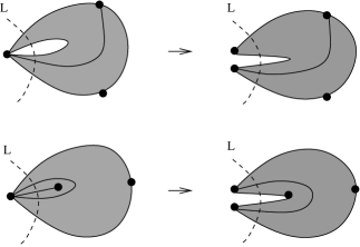
Figure 30.

This completes the proof of the claim, and hence the theorem. ∎

We are now ready to prove Theorem 4.9.

Proof.

We have fixed a bordered surface $(S,M)$, an ordinary arc $\gamma$, and an ideal triangulation $T$ with internal arcs $\tau_{1},\dots,\tau_{n}$ and boundary segments $\tau_{n+1},\dots,\tau_{n+c}$. This determines a cluster algebra $\mathcal{A}$ with principal coefficients with respect to $\Sigma_{T}$. From $(S,M)$, $T$, and $\gamma$ we have built a polygon $\widetilde{S}_{\gamma}$ with a “lift” $\tilde{\gamma}$ of $\gamma$, together with a triangulation $\widetilde{T}_{\gamma}$ with internal arcs $\sigma_{1},\dots,\sigma_{d}$ and boundary segments $\sigma_{d+1},\dots,\sigma_{2d+3}.$ We have a surjective map $\pi:\{\sigma_{1},\dots,\sigma_{2d+3}\}\to\{\tau_{1},\dots,\tau_{n+c}\}$. Furthermore, we have associated a type $A_{d}$ cluster algebra $\widetilde{\mathcal{A}}_{\gamma}$ to $\widetilde{S}_{\gamma}$, and a homomorphism $\phi_{\gamma}$ from $\widetilde{\mathcal{A}}_{\gamma}$ to $\operatorname{Frac}(\mathcal{A})$. This map has the property that for each $\sigma_{i}\in\{\sigma_{1},\dots,\sigma_{2d+3}\}$, $\phi_{\gamma}(x_{\sigma_{i}})=x_{\pi(\sigma_{i})}$. Additionally, by Theorem 10.1, $\phi_{\gamma}(x_{\tilde{\gamma}})=x_{\gamma}$.

Since $\widetilde{\mathcal{A}}_{\gamma}$ is a type A cluster algebra, we can compute the Laurent expansion of $x_{\tilde{\gamma}}$ with respect to $\Sigma_{\widetilde{T}_{\gamma}}$. More specifically, [MS] proved Theorem 4.9 for unpunctured surfaces, which in particular includes polygons. At this point the reader may worry that Theorem 4.9 cannot be applied to $\widetilde{\mathcal{A}}_{\gamma}$, as $\widetilde{\mathcal{A}}_{\gamma}$ is not simply a cluster algebra with principal coefficients associated to a triangulation – it has extra coefficient variables corresponding to the boundary segments of $\widetilde{T}_{\gamma}$. However, consider the triangulated polygon $(\widetilde{S}^{\prime}_{\gamma},\widetilde{T}^{\prime}_{\gamma})$ that we obtain from $(\widetilde{S}_{\gamma},\widetilde{T}_{\gamma})$ by adding $c$ triangles around the boundary, each one with an edge at a boundary segment, and consider the corresponding cluster algebra $\widetilde{\mathcal{A}}^{\prime}_{\gamma}$ with principal coefficients. This is still a type A cluster algebra so we can use the result of [MS] to apply Theorem 4.9 to expand the cluster variable corresponding to $\tilde{\gamma}$ with respect to $\Sigma_{\widetilde{T}^{\prime}_{\gamma}}$ in $\widetilde{\mathcal{A}}^{\prime}_{\gamma}$. And clearly the formula giving the Laurent expansion of $x_{\tilde{\gamma}}$ with respect to $\Sigma_{\widetilde{T}_{\gamma}}$ in $\widetilde{\mathcal{A}}_{\gamma}$ is identical to the formula giving the Laurent expansion of the cluster variable corresponding to $\tilde{\gamma}$ with respect to $\Sigma_{\widetilde{T}^{\prime}_{\gamma}}$ in $\widetilde{\mathcal{A}}^{\prime}_{\gamma}$.

Therefore we can apply Theorem 4.9 to get the cluster expansion of $x_{\tilde{\gamma}}$ with respect to $\Sigma_{\widetilde{T}_{\gamma}}$ in $\widetilde{\mathcal{A}}_{\gamma}$: in other words, we build a graph $G_{\widetilde{T}_{\gamma},\tilde{\gamma}}$, and the cluster expansion is given as a generating function for perfect matchings of this graph. The variables in the expansion are $x_{\sigma_{1}},\dots,x_{\sigma_{2d+3}}$ and $y_{\sigma_{1}},\dots,y_{\sigma_{d}}$. Therefore, since $\phi_{\gamma}$ is a homomorphism such that $\phi_{\gamma}(x_{\sigma_{i}})=x_{\pi(\sigma_{i})}$ for $1\leq i\leq 2d+3$, and $\phi_{\gamma}(x_{\sigma})=x_{\pi(\sigma)}$, computing the Laurent expansion for $x_{\gamma}$ with respect to $T$ in $\mathcal{A}$ amounts to applying a specialization of variables to the generating function for matchings in $G_{\widetilde{T}_{\gamma}}$.

It follows from the construction in Section 7 that the unlabeled graph $G_{\widetilde{T}_{\gamma},\tilde{\gamma}}$ is equal to the unlabeled graph $G_{T,\gamma}$: this is because the triangulated polygon $(\widetilde{S}_{\gamma},\widetilde{T}_{\gamma})$ is built so that the local configuration of triangles that $\tilde{\gamma}$ passes through is the same as the local configuration of triangles that $\gamma$ passes through in $T$. Additionally, an edge of $G_{\widetilde{T}_{\gamma},\tilde{\gamma}}$ labeled $\sigma_{i}$ corresponds to an edge of $G_{T,\gamma}$ labeled $\pi(\sigma_{i})$.

Comparing the definition of $\phi_{\gamma}$ on the coefficients $y_{\sigma_{j}}$ (Equation 8.3) to the definition of the specialized height monomial (Definition 4.8), we see now that applying $\phi_{\gamma}$ to the generating function for matchings in $G_{\widetilde{T}_{\gamma},\tilde{\gamma}}$ yields exactly the formula of Theorem 4.9 applied to $S$, $T$, and $\gamma$. This completes the proof of the theorem. ∎

11. Positivity for notched arcs in the coefficient-free case

In this section we will use Proposition 5.3 together with our positivity result for ordinary arcs to prove the positivity result for notched arcs (in the coefficient-free case). We begin by proving Proposition 5.3.

Proof.

Fix a bordered surface $(S,M)$ and an ideal triangulation $T$ of $S$. Let $\mathcal{A}$ be the associated coefficient-free cluster algebra. Consider a puncture $p$, a different marked point $q$, and an ordinary arc $\gamma$ between $p$ and $q$. Consider a third marked point $s$ and an ordinary arc $\rho$ between $p$ and $s$. Let $\alpha$ and $\beta$ be the two ordinary arcs between $q$ and $s$ which are sides of a bigon so that the triangles with sides $\alpha,\gamma,\rho$ and $\beta,\gamma,\rho$ have simply-connected interior. See the left-hand-side of Figure 31.

Figure 31.

Then in $\mathcal{A}$, $x_{\gamma}x_{\rho^{(p)}}=x_{\alpha}+x_{\beta}=x_{\gamma^{(p)}}x_{\rho}$, which implies that $\frac{x_{\gamma^{(p)}}}{x_{\gamma}}=\frac{x_{\rho^{(p)}}}{x_{\rho}}.$ In other words, the ratio $\frac{x_{\gamma^{(p)}}}{x_{\gamma}}$ is an invariant which we will call $z_{p}$, which depends only on $p$, and not the choice of ordinary arc $\gamma$ incident to $p$.

If we take the same bigon with sides $\alpha$ and $\beta$ and notch all three arcs emanating from $q$, we get $x_{\gamma^{(pq)}}x_{\rho}=x_{\alpha^{(q)}}+x_{\beta^{(q)}}=z_{q}x_{\alpha}+z_{q}x_{\beta}=z_{q}(x_{\gamma^{(p)}}x_{\rho}).$ Therefore $x_{\gamma^{(pq)}}=z_{q}x_{\gamma^{(p)}}=z_{p}z_{q}x_{\gamma}$.

So far we have treated the case where $\gamma$ has two distinct endpoints. Now suppose that $\gamma$ is an ordinary loop based at $p$ which does not cut out a once-punctured monogon. Then choose a marked point $q$ in the interior of $\gamma$, another marked point $s$, and an ordinary arc from $q$ to $s$ which crosses $\gamma$ once. Let $\alpha_{1}$ and $\alpha_{2}$ be ordinary arcs between $p$ and $s$, and $\alpha_{3}$ and $\alpha_{4}$ be ordinary arcs between $p$ and $q$ so that the $\alpha_{i}$ form the sides of a quadrilateral with simply-connected interior. See the right-hand-side of Figure 31. Then $x_{\gamma}x_{\rho}=x_{\alpha_{1}}x_{\alpha_{3}}+x_{\alpha_{2}}x_{\alpha_{4}}$ and $x_{\gamma^{(pp)}}x_{\rho}=x_{\alpha_{1}^{(p)}}x_{\alpha_{3}^{(p)}}+x_{\alpha_{2}^{(p)}}x_{\alpha_{4}^{(p)}}$, where $x_{\alpha_{i}^{(p)}}=z_{p}x_{\alpha_{i}}$. It follows that $x_{\gamma^{(pp)}}=z_{p}^{2}x_{\gamma}$.

What remains is to give an explicit expression for the quantity $z_{p}$. For $\gamma$ an ordinary arc with distinct endpoints, we know that $z_{p}=\frac{x_{\gamma^{(p)}}}{x_{\gamma}}$ does not depend on the choice of $\gamma$, so we make the simplest possible choice. Choose $\tau_{1}$ to be any arc of $T$ which is incident to $p$, so that $x_{\tau_{1}}$ is in the initial cluster associated to $T$. Let $q$ denote the other endpoint of $\tau_{1}$, and let $\ell$ be the loop based at $q$ cutting out a once-punctured monogon around $p$. Then $x_{\ell}=x_{\tau_{1}}x_{\tau_{1}^{(p)}}$, so $z_{p}=\frac{x_{\tau_{1}^{(p)}}}{x_{\tau_{1}}}=\frac{x_{\ell}}{x_{\tau_{1}}^{2}}$. The variable $x_{\tau_{1}}$ is an initial cluster variable and we can compute the Laurent expansion of $x_{\ell}$ using Theorem 4.9.

It is easy to see that the graph $\overline{G}_{\ell,T}$ consists of $h-1$ tiles with diagonals $\tau_{2},\dots,\tau_{h}$, where $\tau_{1},\tau_{2},\dots,\tau_{h}$ are the arcs of $T$ emanating from $p$ (say in clockwise order around $p$). The tiles are glued in an alternating fashion so as to form a “zig-zag” shape, see Figure 32. Also, $\tau_{1}$ is the label of the two outer edges of $\overline{G}_{\ell,T}$. Now a straightforward induction on $h$ shows that applying Theorem 4.9 to $\ell$ gives

$$x_{\ell}=\frac{x_{\tau_{1}}\sum_{i=0}^{h-1}\sigma^{i}(x_{[\tau_{1},\tau_{2}]}x_{\tau_{3}}x_{\tau_{4}}\cdots x_{\tau_{h}})}{x_{\tau_{2}}\cdots x_{\tau_{h}}},$$

where $\sigma$ is the cyclic permutation $(1,2,3,\dots,h)$ acting on subscripts. Dividing this expression by $x_{\tau_{1}}^{2}$ gives the desired expression for $z_{p}$.

Figure 32.

This completes the proof. ∎

Corollary 11.1.

Fix a bordered surface $(S,M)$, a tagged triangulation $T$ of the form $\iota(T^{\circ})$ where $T^{\circ}$ is an ideal triangulation, and let $\mathcal{A}$ be the corresponding coefficient-free cluster algebra. Then the Laurent expansion of a cluster variable corresponding to a notched arc with respect to $\Sigma_{T}$ is positive.

Proof.

This follows immediately from our positivity result for cluster variables corresponding to ordinary arcs, together with Proposition 5.3. ∎

12. Proofs of Laurent expansions for notched arcs

In this section, we prove the results of Section 4.4, giving cluster expansion formulas for cluster variables corresponding to tagged arcs. We use algebraic identities for cluster variables to reduce the proofs of Theorem 4.16 and Theorem 4.20 to combinatorial statements about perfect matchings, $\gamma$-symmetric matchings, and $\gamma$-compatible pairs of matchings.

In particular, for the case of a tagged arc $\gamma^{(p)}$ with a single notch at puncture $p$ (Theorem 4.16), we use the equation $x_{\ell_{p}}=x_{\gamma}x_{\gamma^{(p)}}$ and the fact that Theorem 4.9 gives us matching formulas for two out of three of these terms. For the case of a tagged arc $\gamma^{(pq)}$ with a notch at both ends, punctures $p$ and $q$ (Theorem 4.20), we use an identity (described in Section 12.2) involving $x_{\gamma^{(pq)}}$ and three other cluster variables, where all other terms except $x_{\gamma^{(pq)}}$ have matching formulas from Theorems 4.9 and 4.16. In both of these cases, the fact that the desired matching formulas for $x_{\gamma^{(p)}}$ and $x_{\gamma^{(pq)}}$ satisfy combinatorial identities analogous to the algebraic identities coming from the cluster algebra completes the proofs of Theorems 4.16 and 4.20. Before giving these proofs, we introduce some notation and auxiliary lemmas. We begin by describing the shape of the graph $G_{T^{\circ},\ell_{p}}$ in more detail.

Definition 12.1.

Let $H_{\zeta}$ be the connected subgraph of $G_{T^{\circ},\ell_{p}}$ consisting of the union of the tiles $G_{\zeta_{1}}$ through $G_{\zeta_{e_{p}}}$ (see the notation of Section 4.4 and Figure 8).

Remark 12.2.

It follows from the construction of $G_{T^{\circ},\ell_{p}}$ in Section 4.2 and the fact that $\zeta_{1}$ through $\zeta_{e_{p}}$ all share a single endpoint, that $H_{\zeta}$ contains no consecutive triple of tiles all of which lie in the same row or column.

Remark 12.3.

Since the arcs $\tau_{i_{d}},\zeta_{1},\zeta_{e_{p}}$ are the sides of a triangle in $T^{\circ}$, and $\tau_{i_{d-1}}$ and $\tau_{i_{d}}$ share a vertex, it follows that in the graph $G_{T^{\circ},\ell_{p}}$ either the three tiles $G_{\tau_{i_{d-1}}},G_{\tau_{i_{d}}}$, and $G_{\zeta_{1}}$ or the three tiles $G_{\tau_{i_{d-1}}},G_{\tau_{i_{d}}}$ and $G_{\zeta_{e_{p}}}$ lie in a single row or column. Thus, we may assume without loss of generality that tiles $G_{\tau_{i_{d-1}}}$, $G_{\tau_{i_{d}}}$, and $G_{\zeta_{1}}$ lie in a single row and tiles $G_{\tau_{i_{d-1}}}$, $G_{\tau_{i_{d}}}$, and $G_{\zeta_{e_{p}}}$ do not. See Figure 33.

Lemma 12.4.

If $P$ is a perfect matching of $G_{T^{\circ},\ell_{p}}$ then $P$ restricts to a perfect matching on at least one of its two ends. More precisely, $P|_{G_{T^{\circ},\gamma_{p},1}}$ is a perfect matching of ${G_{T^{\circ},\gamma_{p},1}}$, or the analogous condition must hold for $P|_{G_{T^{\circ},\gamma_{p},2}}$.

Proof.

See Figure 33. We let $w_{1}$ (respectively $w_{2}$) denote the other vertex of the edge labeled $\zeta_{e_{p}}$ (respectively $\zeta_{1}$) incident to $v_{1}$ (respectively $v_{2}$). Suppose that $P$ is a perfect matching of $G_{T^{\circ},\ell_{p}}$ whose restriction to each of the subgraphs $G_{T^{\circ},\gamma_{p},i}$ is not a perfect matching. The restriction of $P$ to $G_{T^{\circ},\gamma_{p},1}$ is not a perfect matching if and only if $P$ contains the edge labeled $\zeta_{2}$ incident to vertex $v_{1}$. Then $P$ must also contain the edge labeled $\tau_{i_{d}}$ on the same tile because otherwise the vertex $w_{1}$ could only be covered by the edge labeled $\tau_{i_{d-1}}$ and this would leave a connected component with an odd number of vertices to match together.

Figure 33. The graph $G_{T^{\circ},\ell_{p}}$. There exists no perfect matching of $G_{T^{\circ},\ell_{p}}$ containing the highlighted edges. Here $e_{p}$ is even.

Similarly, the restriction of $P$ to $G_{T^{\circ},\gamma_{p},2}$ is not a perfect matching if and only if $P$ contains the edge labeled $\zeta_{e_{p}-1}$ incident to vertex $v_{2}$. Then $P$ must also contain the edge labeled $\tau_{i_{d}}$ incident to $w_{2}$ on this same tile. However, no perfect matching $P$ can contain all four of these edges since by Remark 12.2, $H_{\zeta}$ contains no consecutive triple of tiles lying in a single row or column. Thus we have a contradiction. ∎

12.1. Proof of the expansion formula for arcs with a single notch

For the proof of Theorem 4.16, we also need the following fact.

Lemma 12.5.

The minimal matching $P_{-}$ of $G_{T^{\circ},\ell_{p}}$ is a $\gamma$-symmetric matching.

Figure 34. One of the matchings $P_{-}$ and $P_{+}$ of $G_{T^{\circ},\ell_{p}}$ must contain the highlighted edges and is therefore $\gamma$-symmetric. Here $e_{p}$ is odd.

Proof.

Since $P_{-}$ and $P_{+}$ are the unique perfect matchings of $G_{T^{\circ},\ell_{p}}$ using only boundary edges, it follows that exactly one out of $\{P_{-},\,P_{+}\}$, say $P_{\epsilon}$, contains the edge labeled $\tau_{i_{d-1}}$ on the tile $G_{\tau_{i_{d}}}$ containing $v_{1}$. The perfect matching $P_{\epsilon}$ cannot contain the edge labeled $\tau_{i_{d}}$ on the adjacent tiles. As shown in Figure 34, the perfect matching $P_{\epsilon}$ contains other edges on the boundary in an alternating fashion. Since the two ends of $G_{T^{\circ},\ell_{p}}$ are isomorphic, continuing along the boundary in an alternating pattern, we obtain that $P_{\epsilon}$ is $\gamma$-symmetric. Its complement must also be $\gamma$-symmetric, so both $P_{-}$ and $P_{+}$ are $\gamma$-symmetric. ∎

We need to introduce a few more definitions before proving Theorem 4.16.

Definition 12.6.

Let $H_{\zeta}^{(i)}$ denote the induced subgraph obtained after deleting the vertices $v_{i}$, $w_{i}$ of $H_{\zeta}$ and all edges incident to those vertices. Let $G_{\zeta}^{(1)}$ (resp. $G_{\zeta}^{(2)}$) denote the subgraph of $G_{T^{\circ},\ell_{p}}$ which is the union $H_{\zeta}^{(1)}\cup G_{T^{\circ},\gamma_{p},2}$ (resp. $G_{T^{\circ},\gamma_{p},1}\cup H_{\zeta}^{(2)}$). That is, we use a superscript $(i)$ to denote the removal of the $i$th side of a graph.

Definition 12.7 (Symmetric completion).

Fix a perfect matching $P$ of $G_{T^{\circ},\ell_{p}}$, and by Lemma 12.4, assume without loss of generality that $P$ restricts to a perfect matching on $G_{T^{\circ},\gamma_{p},1}$. Therefore $P$ also restricts to a perfect matching on the complement, graph $G_{\zeta}^{(1)}$. We define the symmetric completion $\overline{P}=\overline{P|_{G_{\zeta}^{(1)}}}$ of $P|_{G_{\zeta}^{(1)}}$ to be the unique extension of $P|_{G_{\zeta}^{(1)}}$ to $G_{T^{\circ},\ell_{p}}$ such that $\overline{P}|_{H_{T^{\circ},\gamma_{p},1}}\cong\overline{P}|_{H_{T^{\circ},\gamma_{p},2}}$. (Note that after adding edges to $H_{T^{\circ},\gamma_{p},1}$, only vertex $v_{1}$ is not covered. We add an edge incident to $v_{1}$ based on whether the edge incident to $w_{1}$ labeled $\tau_{i_{d-1}}$ is included so far.) It follows from this construction that the restriction $\overline{P}|_{G_{T^{\circ},\gamma_{p},1}}$ is a perfect matching.

Definition 12.8 (Sets $\mathcal{P}(\gamma)$ and $\mathcal{SP}(\gamma^{(p)})$).

For an ordinary arc $\gamma$ (including loops cutting out once-punctured monogons) we let $\mathcal{P}(\gamma)$ denote the set of perfect matchings of $G_{T^{\circ},\gamma}$, and let $\mathcal{SP}(\gamma^{(p)})$ denote the set of $\gamma$-symmetric matchings of $G_{T^{\circ},\ell_{p}}$.

We now prove Theorem 4.16 by constructing a bijection $\psi$ between pairs $(P_{1},P_{2})$ in $\mathcal{P}(\gamma)\times\mathcal{SP}(\gamma^{(p)})$ and perfect matchings $P_{3}$ in $\mathcal{P}(\ell_{p})$. This bijection will be weight-preserving and height-preserving, in the sense that if $\psi(P_{1},P_{2})=P_{3}$, then $x(P_{1})\overline{x}(P_{2})=x(P_{3})$ and $h(P_{1})\overline{h}(P_{2})=h(P_{3})$. This gives

(12.1) $$\sum_{P_{3}\in\mathcal{P}(\ell_{p})}x(P_{3})h(P_{3})=\left(\sum_{P_{1}\in\mathcal{P}(\gamma)}x(P_{1})h(P_{1})\right)\,\left(\sum_{P_{2}\in\mathcal{SP}(\gamma^{(p)})}\overline{x}(P_{2})\overline{h}(P_{2})\right).$$

After applying $\Phi$, the left-hand-side and first term on the right are the numerators for $x_{\ell_{p}}$ and $x_{\gamma}$ given by Theorem 4.9, which allows us to express $x_{\gamma^{(p)}}=\frac{x_{\ell_{p}}}{x_{\gamma}}$ in terms of $\sum_{P_{2}\in\mathcal{SP}(\gamma^{(p)})}\overline{x}(P_{2})\overline{h}(P_{2})$.

Proof of Theorem 4.16.

As indicated above, we define a map

$$\psi:\mathcal{P}(\gamma)\times\mathcal{SP}(\gamma^{(p)})\rightarrow\mathcal{P}(\ell_{p})\mathrm{~{}~{}by}$$

$$\psi(P_{1},P_{2})=\begin{cases}P_{1}~{}\bigcup~{}P_{2}|_{G_{\zeta}^{(1)}}\mathrm{~{}~{}~{}~{}if~{}}P_{2}|_{G_{T^{\circ},\gamma_{p},1}}\mathrm{~{}is~{}a~{}perfect~{}matching}\\ P_{2}|_{G_{\zeta}^{(2)}}~{}\bigcup~{}P_{1}\mathrm{~{}otherwise~{}}\end{cases}$$

where the edges of $P_{1}$ are placed on the subgraph $G_{T^{\circ},\gamma_{p},1}$ or $G_{T^{\circ},\gamma_{p},2}$, respectively. In words, $\psi$ removes all of the edges from one of the two ends of the $\gamma$-symmetric matching $P_{2}$, and replaces those edges with edges from the perfect matching $P_{1}$, thereby constructing a perfect matching $P_{3}$ of $\mathcal{P}(\ell_{p})$ that it is not necessarily $\gamma$-symmetric. By Lemma 12.4, either $P_{2}|_{G_{T^{\circ},\gamma_{p},1}}$ or $P_{2}|_{G_{T^{\circ},\gamma_{p},2}}$ is a perfect matching and so $\psi$ is well-defined. Thus $\psi(P_{1},P_{2})$ is a perfect matching of $\mathcal{P}(\ell_{p})$.

We show that $\psi$ is a bijection by exhibiting its inverse. For $P_{3}\in\mathcal{P}(\ell_{p})$, define

$$\varphi(P_{3})=\begin{cases}(P_{3}|_{G_{T^{\circ},\gamma_{p},1}}~{}~{},~{}~{}\overline{P_{3}|_{G_{\zeta}^{(1)}}})\mathrm{~{}~{}~{}if~{}}P_{3}|_{G_{T^{\circ},\gamma_{p},1}}\mathrm{~{}is~{}a~{}perfect~{}matching},\\ (P_{3}|_{G_{T^{\circ},\gamma_{p},2}}~{}~{},~{}~{}\overline{P_{3}|_{G_{\zeta}^{(2)}}})\mathrm{~{}otherwise.}\end{cases}$$

A little thought shows that these two maps are inverses.

We now show that the bijection $\psi$ is weight-preserving. Without loss of generality, $P_{2}|_{G_{T^{\circ},\gamma_{p},1}}$ is a perfect matching. If $\psi(P_{1},P_{2})=P_{3}$, then $P_{3}=P_{1}~{}\cup~{}P_{2}|_{G_{\zeta}^{(1)}}$. We obtain

$$x(P_{3})=x(P_{1})\,x(P_{2}|_{G_{\zeta}^{(1)}})=x(P_{1})\,\frac{x(P_{2})}{x(P_{2}|_{G_{T^{\circ},\gamma_{p},1}})}.$$

Since $\overline{x}(P_{2})$ is defined to be $\frac{x(P_{2})}{x(P_{2}|_{G_{T^{\circ},\gamma_{p},1}})}$, we conclude that $\psi$ is weight-preserving.

To see that $\psi$ is height-preserving, we use Lemma 12.5, which states that $P_{-}(G_{T^{\circ},\ell_{p}})$ is a $\gamma$-symmetric matching. Consequently, using the same partitioning that showed that $\psi$ was weight-preserving, we can consider the following equation describing the symmetric difference of $P_{3}$ and $P_{-}(G_{T^{\circ},\ell_{p}})$:

$$P_{3}\ominus P_{-}(G_{T^{\circ},\ell_{p}})=(P_{1}\ominus P_{-}(G_{T^{\circ},\gamma}))\cup(P_{2}\ominus P_{-}(G_{T^{\circ},\ell_{p}})|_{G_{\zeta}^{(1)}}).$$

Since the cycles appearing in the symmetric difference determine the height monomials, this decomposition implies that

$$h(P_{3})=h(P_{1})\,h(P_{2}|_{G_{\zeta}^{(1)}})=h(P_{1})\,\frac{h(P_{2})}{h(P_{2}|_{G_{T^{\circ},\gamma_{p},1}})}=h(P_{1})\,\overline{h}(P_{2}),$$

hence $\psi$ is height-preserving.

Because $\phi$ is weight- and height-preserving, we have (12.1). Applying $\Phi$ gives

(12.2) $$\sum_{P\in\mathcal{P}(\ell_{p})}x(P)y(P) = \left(\sum_{P_{1}\in\mathcal{P}(\gamma)}x(P_{1})y(P_{1})\right)\left(\sum_{P_{2}\in\mathcal{SP}(\gamma^{(p)})}\overline{x}(P_{2})\overline{y}(P_{2})\right).$$

We now use the identity $x_{\ell_{p}}=x_{\gamma}x_{\gamma^{(p)}}$ and obtain

(12.3) $$x_{\gamma^{(p)}} = \frac{\mathrm{cross}(T^{\circ},\gamma)\sum_{P\in\mathcal{P}(\ell_{p})}x(P)y(P)}{\mathrm{cross}(T^{\circ},\ell_{p})\sum_{P\in\mathcal{P}(\gamma)}x(P)y(P)}.$$

Comparing (12.3) and (12.2) yields the desired formula. ∎

12.2. An algebraic identity for arcs with two notches

We now give the algebraic portion of the proof of Theorem 4.20. For the purpose of computing the Laurent expansion of $x_{\rho^{(pq)}}$ with respect to $T$, we can assume that no tagged arc in $T$ is notched at either $p$ or $q$, see Remark 4.11. In the statement below, the notation $\chi$ indicates $1$ or $0$, based on whether it’s argument is true or false.

Theorem 12.9.

Fix a tagged triangulation $T$ of $(S,M)$ which comes from an ideal triangulation, and let $\mathcal{A}$ be the cluster algebra associated to $(S,M)$ with principal coefficients with respect to $T$. Let $p$ and $q$ be punctures in $S$, and let $\rho$ be an ordinary arc between $p$ and $q$. Assume that no tagged arc in $T$ is notched at either $p$ or $q$. Then

$$x_{\rho}x_{\rho^{(pq)}}-x_{\rho^{(p)}}x_{\rho^{(q)}}y_{\rho}^{\chi(\rho\in T)}=(1-\prod_{\tau\in T}y_{\tau}^{e_{p}(\tau)})(1-\prod_{\tau\in T}y_{\tau}^{e_{q}(\tau)})\prod_{\tau\in T}y_{\tau}^{e(\tau,\rho)}.$$

Proof.

For simplicity, we assume for now that $\rho\notin T$. (Later we will lift the assumption.) Choose a quadrilateral in $S$ with simply connected interior such that one of its diagonals is $\rho$. (This involves the choice of two more marked points, say $v$ and $w$.) Label the (ordinary) arcs of the quadrilateral by $\alpha,\beta,\gamma,\delta$ and the other diagonal by $\rho^{\prime}$, as in Figure 35. Note that there are four ways of changing the taggings around $p$ and $q$, and for each we get a Ptolemy relation.

Figure 35.

(12.4) $$x_{\rho}x_{\rho^{\prime}} =Y^{+}Y_{q}^{+}Y_{p}^{+}x_{\beta}x_{\delta}+Y^{-}x_{\alpha}x_{\gamma}$$

(12.5) $$x_{\rho^{(p)}}x_{\rho^{\prime}} =Y^{+}Y_{q}^{+}x_{\beta}x_{\delta^{(p)}}+Y^{-}Y_{p}^{-}x_{\alpha^{(p)}}x_{\gamma}$$

(12.6) $$x_{\rho^{(q)}}x_{\rho^{\prime}} =Y^{+}Y_{p}^{+}x_{\beta^{(q)}}x_{\delta}+Y^{-}Y_{q}^{-}x_{\alpha}x_{\gamma^{(q)}}$$

(12.7) $$x_{\rho^{(pq)}}x_{\rho^{\prime}} =Y^{+}x_{\beta^{(q)}}x_{\delta^{(p)}}+Y^{-}Y_{q}^{-}Y_{p}^{-}x_{\alpha^{(p)}}x_{\gamma^{(q)}}$$

Here, $Y^{+}$ (respectively $Y^{-}$) is the monomial (in coefficient variables) coming from all laminations which do not spiral into $p$ or $q$ and which give a shear coordinate of $1$ (respectively $-1$) with $\rho$, as in Figure 39. We use Definition 12.1 of [FT] to compute shear coordinates with respect to tagged arcs $\rho^{(p)}$, $\rho^{(q)}$, and $\rho^{(pq)}$.

$Y_{p}^{\pm}$ and $Y_{q}^{\pm}$ are monomials coming from laminations which spiral into either the puncture $p$ or $q$, respectively. Since we have assumed that $T$ does not contain arcs with a notch at $p$ or $q$, all laminates which spiral into $p$ or $q$ spiral counterclockwise. $Y_{p}^{+}$ is the monomial coming from laminations that spiral into $p$ giving a shear coordinate of $1$ to $\rho$ (equivalently, a shear coordinate of $1$ to $\rho^{(q)}$). $Y_{q}^{+}$ is the monomial coming from laminations that spiral into $q$ giving a shear coordinate of $1$ to $\rho$ (equivalently, a shear coordinate of $1$ to $\rho^{(p)}$). $Y_{p}^{-}$ is the monomial coming from laminations that spiral into $p$ giving a shear coordinate of $-1$ to $\rho^{(p)}$ (equivalently, to $\rho^{(pq)}$). Finally, $Y_{q}^{-}$ is the monomial coming from laminations that spiral into $q$ giving a shear coordinate of $-1$ to $\rho^{(q)}$ (equivalently, to $\rho^{(pq)}$). See Figure 36.

Figure 36.

When we multiply equations (12.4) and (12.7) and subtract the product of (12.5) and (12.6), some terms cancel. Factoring the remaining terms, we find that

$$(x_{\rho^{\prime}})^{2}(x_{\rho}x_{\rho^{(pq)}}-x_{\rho^{(p)}}x_{\rho^{(q)}})=Y^{+}Y^{-}(Y_{p}^{+}Y_{p}^{-}x_{\alpha^{(p)}}x_{\delta}-x_{\alpha}x_{\delta^{(p)}})(Y_{q}^{+}Y_{q}^{-}x_{\gamma^{(q)}}x_{\beta}-x_{\beta^{(q)}}x_{\gamma}).$$

We now want to interpret each of the terms $x_{\alpha^{(p)}}x_{\delta}$, $x_{\alpha}x_{\delta^{(p)}}$, $x_{\gamma^{(q)}}x_{\beta}$, and $x_{\beta^{(q)}}x_{\gamma}$ as the left-hand-side of a Ptolemy relation. To this end, let $\epsilon$ be the arc between $v$ and $w$ which is homotopic to the concatenation of $\alpha$ and $\delta$, so that $\epsilon$ and $\rho^{\prime}$ are opposite sides of a bigon with vertices $v$ and $w$ and internal vertex $p$. See Figure 37.

Figure 37.

The Ptolemy relations concerning this bigon are

$$x_{\alpha}x_{\delta^{(p)}} =Y_{2}Y_{4}x_{\epsilon}+Y_{1}x_{\rho^{\prime}}$$

$$x_{\delta}x_{\alpha^{(p)}} =Y_{1}Y_{3}x_{\rho^{\prime}}+Y_{2}x_{\epsilon}.$$

Here $Y_{1},Y_{2},Y_{3}$, and $Y_{4}$ are monomials coming from laminations that intersect $\alpha$ and $\delta$ as in Figure 38.

Figure 38.

(See also [FT, Figure 32].) Note that by our assumptions on $T$, we do not have to worry about laminations that spiral clockwise into $p$.

A laminate crossing $\rho^{\prime}$ and spiraling to $p$ must cross $\rho$, so $Y_{p}^{+}Y_{p}^{-}=Y_{4}$. Therefore

$$Y_{p}^{+}Y_{p}^{-}x_{\alpha^{(p)}}x_{\delta}-x_{\alpha}x_{\delta^{(p)}} =Y_{4}(Y_{1}Y_{3}x_{\rho^{\prime}}+Y_{2}x_{\epsilon})-(Y_{2}Y_{4}x_{\epsilon}+Y_{1}x_{\rho^{\prime}})$$

$$=Y_{1}x_{\rho^{\prime}}(Y_{3}Y_{4}-1)$$

$$=Y_{1}x_{\rho^{\prime}}(\prod_{\tau\in T}y_{\tau}^{e_{p}(\tau)}-1),$$

since laminates spiraling to $p$ correspond to tagged arcs incident to $p$.

Similarly, letting $\eta$ be the arc between $v$ and $w$ homotopic to the concatenation of $\beta$ and $\gamma$, so that $\rho^{\prime}$ and $\eta$ are opposite sides of a bigon with the interior point $q$, we get the following Ptolemy relations.

$$x_{\beta}x_{\gamma^{(q)}} =Y_{2}^{\prime}Y_{4}^{\prime}x_{\rho^{\prime}}+Y_{1}^{\prime}x_{\eta}$$

$$x_{\gamma}x_{\beta^{(q)}} =Y_{1}^{\prime}Y_{3}^{\prime}x_{\eta}+Y_{2}^{\prime}x_{\rho^{\prime}}.$$

Here, $Y_{1}^{\prime},Y_{2}^{\prime},Y_{3}^{\prime},Y_{4}^{\prime}$ are defined just as $Y_{1},Y_{2},Y_{3},Y_{4}$ were, with $q$ replacing $p$.

Similar to above, $Y_{q}^{+}Y_{q}^{-}=Y_{3}^{\prime}$, and

$$Y_{q}^{+}Y_{q}^{-}x_{\gamma^{(q)}}x_{\beta}-x_{\beta^{(q)}}x_{\gamma}=Y_{2}^{\prime}x_{\rho^{\prime}}(\prod_{\tau\in T}y_{\tau}^{e_{q}(\tau)}-1).$$

We now have that

$$(x_{\rho^{\prime}})^{2}(x_{\rho}x_{\rho^{(pq)}}-x_{\rho^{(p)}}x_{\rho^{(q)}})=Y^{+}Y^{-}Y_{1}x_{\rho^{\prime}}(\prod_{\tau\in T}y_{\tau}^{e_{p}(\tau)}-1)Y_{2}^{\prime}x_{\rho^{\prime}}(\prod_{\tau\in T}y_{\tau}^{e_{q}(\tau)}-1),$$

so

$$x_{\rho}x_{\rho^{(pq)}}-x_{\rho^{(p)}}x_{\rho^{(q)}}=Y^{+}Y^{-}Y_{1}Y_{2}^{\prime}(\prod_{\tau\in T}y_{\tau}^{e_{p}(\tau)}-1)(\prod_{\tau\in T}y_{\tau}^{e_{q}(\tau)}-1).$$

Since the monomials $Y^{\pm},Y_{1}$ and $Y_{2}^{\prime}$ are defined by laminates crossing the quadrilateral as in Figure 39 (which in turn come from tagged arcs of $T$ that have the same local configuration), it follows that

$$Y^{+}Y^{-}Y_{1}Y_{2}^{\prime}=\prod_{\tau\in T}y_{\tau}^{e(\tau,\rho)}.$$

This completes the proof when $\rho\notin T$.

Figure 39.

If $\rho\in T$, the proof is nearly the same. In this case, one gets a contribution to the shear coordinates from the laminate $L_{\rho}$ associated to $\rho$, see Figure 35. Equations (12.5) and (12.6) remain the same, and equations (12.4) and (12.7) become

(12.8) $$x_{\rho}x_{\rho^{\prime}} =Y^{+}Y_{q}^{+}Y_{p}^{+}y_{\rho}x_{\beta}x_{\delta}+Y^{-}x_{\alpha}x_{\gamma}$$

(12.9) $$x_{\rho^{(pq)}}x_{\rho^{\prime}} =Y^{+}x_{\beta^{(q)}}x_{\delta^{(p)}}+Y^{-}Y_{q}^{-}Y_{p}^{-}y_{\rho}x_{\alpha^{(p)}}x_{\gamma^{(q)}}.$$

Using the four Ptolemy relations, i.e. (12.8)(12.9) $-y_{\rho}$(12.5)(12.6), we get

$$x_{\rho^{\prime}}^{2}(x_{\rho}x_{\rho^{(pq)}}-y_{\rho}x_{\rho^{(p)}}x_{\rho^{(q)}})=Y^{+}Y^{-}(y_{\rho}Y_{p}^{+}Y_{p}^{-}x_{\alpha^{(p)}}x_{\delta}-x_{\alpha}x_{\delta^{(p)}})(y_{\rho}Y_{q}^{+}Y_{q}^{-}x_{\gamma^{(q)}}x_{\beta}-x_{\beta^{(q)}}x_{\gamma}).$$

In this case $y_{\rho}Y_{p}^{+}Y_{p}^{-}=Y_{4}$ and $y_{\rho}Y_{q}^{+}Y_{q}^{-}=Y_{3}^{\prime}$, and the proof continues as before. ∎

There is a version of Theorem 12.9 which makes no assumptions on the notching of arcs in $T$ at $p$ or $q$. Although we won’t use it later, we record the statement.

Theorem 12.10.

Fix a tagged triangulation $T$ of $(S,M)$ which comes from an ideal triangulation, and let $\mathcal{A}$ be the cluster algebra associated to $(S,M)$ with principal coefficients with respect to $T$. Let $p$ and $q$ be punctures in $S$, and let $\rho$ be an ordinary arc between $p$ and $q$. Then

$$x_{\rho}x_{\rho^{(pq)}}y_{\rho^{(p)}}^{\chi(\rho^{(p)}\in T)}y_{\rho^{(q)}}^{\chi(\rho^{(q)}\in T)}-x_{\rho^{(p)}}x_{\rho^{(q)}}y_{\rho}^{\chi(\rho\in T)}y_{\rho^{(pq)}}^{\chi(\rho^{(pq)}\in T)}$$

is equal to

$$\prod_{\tau\in T}y_{\tau}^{e(\tau,\rho)}(\prod_{\tau\in T}y_{\tau}^{e_{p}^{\bowtie}(\tau)}-\prod_{\tau\in T}y_{\tau}^{e_{p}(\tau)})(\prod_{\tau\in T}y_{\tau}^{e_{q}^{\bowtie}(\tau)}-\prod_{\tau\in T}y_{\tau}^{e_{q}(\tau)}),$$

where $e_{p}(\tau)$ (respectively, $e_{p}^{\bowtie}(\tau)$) is the number of ends of $\tau$ that are incident to the puncture $p$ with an ordinary (respectively, notched) tagging.

Remark 12.11.

In the degenerate case of a bordered surface with two punctures $p$ and $q$ and only one other marked point $v$, Theorem 12.9 still holds and the proof is analogous. Here we let $\rho^{\prime}$ be a loop based at $v$ crossing $\rho$ exactly once, and define $\alpha$, $\beta=\gamma$, and $\delta$ as in Figure 40. Note that we can view $\alpha,\beta,\gamma,$ and $\delta$ as the four sides of a degenerate quadrilateral with diagonals $\rho$ and $\rho^{\prime}$. We then obtain the analogues of equations (12.4)-(12.9), replacing all instances of vertex $w$ with $v$, $\gamma$ with $\beta$, $x_{\beta}x_{\beta^{(p)}}$ with $x_{\rho^{\prime}}$, $Y_{2}^{\prime}$ with $1$, and $Y_{q}^{+}Y_{q}^{-}$ with $\prod_{\tau\in T}y_{\tau}^{e_{q}(\tau)}$.

Figure 40.

Remark 12.12.

In the degenerate case when $p=q$, Theorem 12.9 also holds, but we need to make sense of notation such as $x_{\rho^{(p)}}$ when $\rho$ is a loop. See Section 12.4.

12.3. Combinatorial identities satisfied by $\gamma$-compatible pairs of matchings

We now use Theorem 12.9 to prove Proposition 4.21, where $\gamma\in T^{\circ}$, and then Theorem 4.20, where $\gamma\not\in T^{\circ}$. In both proofs, we will use Theorems 4.9 and 4.16 to replace appearances of cluster variables $x_{\gamma}$, $x_{\gamma^{(p)}}$, and $x_{\gamma^{(q)}}$ with generating functions of perfect (and $\gamma$-symmetric) matchings of graphs $G_{T^{\circ},\gamma}$, $G_{T^{\circ},\ell_{p}}$ and $G_{T^{\circ},\ell_{q}}$. We are then reduced to proving combinatorial identities concerning these sets of matchings.

Lemma 12.13.

Assume that the ideal triangulation $T^{\circ}$ contains the arc $\gamma$ between the punctures $q$ and $p$ ($p\not=q$). Let $\ell_{p}$ denote the loop based at puncture $q$ enclosing the arc $\gamma$ and puncture $p$, but no other marked points. Let $P_{-}(\ell_{p})$ and $P_{+}(\ell_{p})$ denote the minimal and maximal matchings of $G_{T^{\circ},\ell_{p}}$, respectively. Define $\ell_{q}$, $P_{-}(\ell_{q})$, and $P_{+}(\ell_{q})$ analogously. Assume the local configuration around arc $\gamma$ and punctures $p$ and $q$ is as in Figure 41. Let $\zeta_{1}=\gamma$ and $\zeta_{2}$ through $\zeta_{e_{p}}$ label the arcs that $\ell_{p}$ crosses as we follow it clockwise around puncture $p$. Analogously, let $\eta_{1}=\gamma$ and $\eta_{2}$ through $\eta_{e_{q}}$ label the arcs that $\ell_{q}$ crosses as we follow it clockwise around puncture $q$. Then we have the following.

Figure 41. The local configuration around arc $\gamma$ between $p$ and $q$.

(12.10) $$x(P_{-}(\ell_{p}))\,h(P_{-}(\ell_{p})) = x_{\gamma}\big{(}\prod_{j=2}^{e_{p}-1}x_{\zeta_{j}}\big{)}x_{\eta_{2}},$$

(12.11) $$x(P_{+}(\ell_{p}))\,h(P_{+}(\ell_{p})) = x_{\eta_{e_{q}}}\big{(}\prod_{j=3}^{e_{p}}x_{\zeta_{j}}\big{)}x_{\gamma}\big{(}\prod_{j=2}^{e_{p}}h_{\zeta_{j}}\big{)}.$$

There are analogous identies for $\ell_{q}$, which we get by replacing $p$ with $q$ and switching the $\eta$’s and $\zeta$’s.

Proof.

The minimal and maximal matchings are precisely those that contain only boundary edges. We distinguish between the two based on the fact that arcs $\zeta_{e_{p}}$, $\gamma$, and $\zeta_{2}$ are assumed to be given in clockwise order, as are $\eta_{e_{q}}$, $\gamma$, and $\eta_{2}$. The edges of the minimal and maximal matchings both have a regular alternating pattern on the interior of $H_{\zeta}$ (resp. $H_{\eta}$). See Figure 42 for the verification of equation (12.10). The weights in the other equation are analogous.

Figure 42. The graph $G_{T^{\circ},\ell_{p}}$ with the minimal matching $P_{-}(\ell_{p})$ highlighted.

The height monomial of a minimal matching is $1$, and the height monomial of a maximal matching of a graph is the product of $h_{\tau_{i}}$’s, one for each label of a tile in the graph. Thus, looking at the diagonals (i.e. labels) of the tiles in $G_{T^{\circ},\ell_{p}}$ and $G_{T^{\circ},\ell_{q}}$ completes the proof. ∎

Proof of Proposition 4.21.

We define $\zeta_{1}$ through $\zeta_{e_{p}}$ and $\eta_{1}$ through $\eta_{e_{q}}$ as in Lemma 12.13. Based on Lemma 12.13, it follows that

$$x(P_{-}(\ell_{q}))\,h(P_{-}(\ell_{q}))\,x(P_{+}(\ell_{p}))\,h(P_{+}(\ell_{p}))\,h_{\gamma} = x_{\gamma}^{2}h_{\gamma}\prod_{j=2}^{e_{p}}(x_{\zeta_{j}}h_{\zeta_{j}})\prod_{j=2}^{e_{q}}x_{\eta_{j}}\hskip 15.00002pt\mathrm{~{}and}$$

$$x(P_{-}(\ell_{p}))\,h(P_{-}(\ell_{p}))\,x(P_{+}(\ell_{q}))\,h(P_{+}(\ell_{q}))\,h_{\gamma} = x_{\gamma}^{2}h_{\gamma}\prod_{j=2}^{e_{p}}x_{\zeta_{j}}\prod_{j=2}^{e_{q}}(x_{\eta_{j}}h_{\eta_{j}}).$$

$$\text{Therefore }\frac{\sum_{P_{p}\in\mathcal{P}(\ell_{p})}x(P_{p})\,h(P_{p})}{x_{\gamma}x_{\zeta_{2}}x_{\zeta_{3}}\cdots x_{\zeta_{e_{p}}}}\cdot\frac{\sum_{P_{q}\in\mathcal{P}(\ell_{q})}x(P_{q})\,h(P_{q})}{x_{\gamma}x_{\eta_{2}}x_{\eta_{3}}\cdots x_{\eta_{e_{q}}}}\cdot h_{\gamma}$$

$$- h_{\gamma}\big{(}\prod_{j=2}^{e_{p}}h_{\zeta_{j}}\big{)}-h_{\gamma}\big{(}\prod_{j=2}^{e_{q}}h_{\eta_{j}}\big{)}+1+h_{\gamma}^{2}\big{(}\prod_{j=2}^{e_{p}}h_{\zeta_{j}}\big{)}\big{(}\prod_{j=2}^{e_{q}}h_{\eta_{j}}\big{)}$$

is positive, since $P_{\pm}(\ell_{p})\in\mathcal{P}(\ell_{p})$, $P_{\pm}(\ell_{q})\in\mathcal{P}(\ell_{q})$, and thus the two negative terms cancel with terms coming from the product of Laurent polynomials.

Since we assumed that $T$ does not contain any arcs with notches at $p$ or $q$, it follows that $\Phi(h_{\gamma})=y_{\gamma}$, $\Phi(h(P_{p}))=y(P_{p})$, $\prod_{j=2}^{e_{p}}\Phi(h_{\zeta_{j}})=\prod_{\tau\in T}y_{\tau}^{e_{p}(\tau)}$, and $\prod_{j=2}^{e_{q}}\Phi(h_{\eta_{j}})=\prod_{\tau\in T}y_{\tau}^{e_{q}(\tau)}$. Applying $\Phi$ to (12.3), we obtain that

(12.13) $$\frac{\sum_{P_{p}\in\mathcal{P}(\ell_{p})}x(P_{p})\,y(P_{p})}{x_{\gamma}x_{\zeta_{2}}x_{\zeta_{3}}\cdots x_{\zeta_{e_{p}}}}\cdot\frac{\sum_{P_{q}\in\mathcal{P}(\ell_{q})}x(P_{q})\,y(P_{q})}{x_{\gamma}x_{\eta_{2}}x_{\eta_{3}}\cdots x_{\eta_{e_{q}}}}\cdot y_{\gamma}+(1-\prod_{\tau\in T}y_{\tau}^{e_{p}(\tau)})(1-\prod_{\tau\in T}y_{\tau}^{e_{q}(\tau)})$$

is positive. Since $\gamma\in T$, $x_{\gamma}$ is an initial cluster variable and the left-hand-side of (12.13) can be rewritten using Remark 4.17. Theorem 12.9 then gives

$$x_{\gamma^{(pq)}} = \frac{x_{\gamma^{(p)}}x_{\gamma^{(q)}}y_{\gamma}+\big{(}1-\prod_{\tau\in T}y_{\tau}^{e_{p}(\tau)}\big{)}\big{(}1-\prod_{\tau\in T}y_{\tau}^{e_{q}(\tau)}\big{)}}{x_{\gamma}}.$$

It follows that the cluster expansion of $x_{\gamma^{(pq)}}$ is positive. ∎

For the remainder of this section, we assume that $\gamma$ (as well as $\gamma^{(p)},\gamma^{(q)}$ and $\gamma^{(pq)}$) is not in the tagged triangulation $T$. We use the notation of Definition 12.8, and additionally we let $\mathcal{CP}(\gamma^{(pq)})$ denote the set of pairs of $\gamma$-compatible matchings $(P_{p},P_{q})$ of $G_{T^{\circ},\ell_{p}}\sqcup G_{T^{\circ},\ell_{q}}$, and let $\mathcal{P}(\zeta)$ (resp. $\mathcal{P}(\zeta^{(i)})$, $\mathcal{P}(\eta)$, and $\mathcal{P}(\eta^{(i)})$) denote the set of perfect matchings of $H_{\zeta}$ (resp. $H_{\zeta}^{(i)}$, $H_{\eta}$, and $H_{\eta}^{(i)}$). Following Section 4.4, we label the tiles of $G_{T^{\circ},\ell_{p}}$ so that they match the labels of the arcs crossed as we travel along $\ell_{p}$ in clockwise order:

$$G_{\tau_{i_{1}}},G_{\tau_{i_{2}}},\dots,G_{\tau_{i_{d}}},G_{\zeta_{1}},G_{\zeta_{2}},\dots,G_{\zeta_{e_{p}-1}},G_{\zeta_{e_{p}}},G_{\tau_{i_{d}}},G_{\tau_{i_{d-1}}},\dots,G_{\tau_{i_{2}}},G_{\tau_{i_{1}}}.$$

See Figure 8. Analogously, the tiles of $G_{T^{\circ},\ell_{q}}$ are labeled so that they match the arcs crossed as we travel along $\ell_{q}$ in clockwise order:

$$G_{\tau_{i_{d}}},G_{\tau_{i_{d-1}}},\dots,G_{\tau_{i_{1}}},G_{\eta_{1}},G_{\eta_{2}},\dots,G_{\eta_{e_{q}-1}},G_{\eta_{e_{q}}},G_{\tau_{i_{1}}},G_{\tau_{i_{2}}},\dots,G_{\tau_{i_{d-1}}},G_{\tau_{i_{d}}}.$$

It follows that the tiles $G_{\tau_{i_{d}}}$ in both $G_{T^{\circ},\ell_{p}}$ and $G_{T^{\circ},\ell_{q}}$ have two adjacent sides labeled $\zeta_{1}$ and $\zeta_{e_{p}}$, and the tiles $G_{\tau_{i_{1}}}$ contain two adjacent sides labeled $\eta_{1}$ and $\eta_{e_{q}}$.

We let $J_{T^{\circ},\gamma_{p},i}$ denote the induced subgraph obtained from $G_{T^{\circ},\gamma_{p},i}$ by deleting vertices $v_{i}$ and $w_{i}$, and all edges incident to either of these two vertices.

Lemma 12.14.

If $P$ is a $\gamma$-symmetric matching of $G_{T^{\circ},\ell_{p}}$ then $P$ can be partitioned into three perfect matchings of subgraphs in exactly one of the two following ways:

1. $P=P|_{G_{T^{\circ},\gamma_{p},1}}\sqcup P|_{H_{\zeta}^{(1)}}\sqcup P|_{J_{T^{\circ},\gamma_{p},2}}$, or

2. $P=P|_{J_{T^{\circ},\gamma_{p},1}}\sqcup P|_{H_{\zeta}^{(2)}}\sqcup P|_{G_{T^{\circ},\gamma_{p},2}}$.

Proof.

See Figures 33 and 34. We will divide the set of $\gamma$-symmetric matchings of $G_{T^{\circ},\ell_{p}}$ into two classes, depending on whether or not they contain one of the edges labeled $\tau_{i_{d-1}}$ on the tiles containing vertex $v_{1}$ and $v_{2}$. By definition, a $\gamma$-symmetric matching must contain both of these edges or neither.

(1) If $P$ contains the specified edges, then $P$ must also contain the edge labeled $\zeta_{1}$ that is incident to vertex $v_{1}$. (Otherwise, vertex $v_{1}$ could only be covered by the edge labeled $\zeta_{2}$ and this would leave a connected component with an odd number of vertices to match together.) Filling in the rest of the edges on tiles $G_{\tau_{i_{1}}}$ through $G_{\tau_{i_{d-1}}}$, we see that $P|_{G_{T^{\circ},\gamma_{p},1}}$ is a perfect matching. Such a $P$ does not contain the edge labeled $\tau_{i_{d}}$ on the tile $G_{\tau_{i_{d-1}}}$ since that would also leave a connected component with an odd number of vertices. Consequently, vertices $v_{2}$ and $w_{2}$ must be covered by edges from the tile $G_{\zeta_{e_{p}}}$. We conclude that the remainder of the set $P$ can be decomposed disjointly as the perfect matchings $P|_{H_{\zeta}^{(1)}}$ and $P|_{J_{T^{\circ},\gamma_{p},2}}$.

(2) If $P$ does not contain the specified edges, then $P$ must contain the edge labeled $\zeta_{e_{p}}$ that is incident to $v_{2}$. (Otherwise the vertex where edges labeled $\zeta_{e_{p}}$ and $\tau_{i_{d-1}}$ meet on that tile would not be covered by an edge of $P$.) Filling in the rest of $P$, we see that it restricts to a perfect matching on $G_{T^{\circ},\gamma_{p},2}$. Since the edge labeled $\tau_{i_{d-1}}$ incident to $w_{1}$ is not in $P$, the edge $\zeta_{1}$ incident to $v_{1}$ cannot be contained in $P$. (Otherwise vertex $w_{1}$ could only be covered by the edge labeled $\tau_{i_{d}}$ and this also leaves an odd number of vertices to match together.) We conclude that the rest of the set $P$ can be decomposed disjointly as the perfect matchings $P|_{J_{T^{\circ},\gamma_{p},1}}$ and $P|_{H_{\zeta}^{(2)}}$.

As $P$ either contains or does not contain the specified edges, the proof is complete. ∎

Remark 12.15.

By Lemma 12.14, it is impossible for both the edge labeled $\zeta_{1}$ incident to $v_{1}$ (resp. $v_{2}$) and the edge labeled $\zeta_{e_{p}}$ incident to $v_{2}$ (resp. $v_{1}$) to appear in a $\gamma$-symmetric matching of $G_{T^{\circ},\ell_{p}}$. Furthermore Case (1) of Lemma 12.14 corresponds to the case where $P$ contains one edge labeled $\zeta_{1}$ incident to $v_{1}$ or $v_{2}$, but does not contain either edge labeled $\zeta_{e_{p}}$ incident to $v_{1}$ or $v_{2}$. Case (2) is the reverse, and analogous statements hold for edges labeled $\eta_{1}$ and $\eta_{e_{q}}$ in $G_{T^{\circ},\ell_{q}}$.

We use this observation to partition various sets of matchings into disjoint sets.

Definition 12.16 ($\mathcal{P}_{a,b}(\gamma)$, $\mathcal{SP}_{a,b}(\gamma^{(p)})$, and $\mathcal{CP}_{a,b}(\gamma^{(pq)})$).

For $a\in\{1,e_{p}\}$ and $b\in\{1,e_{q}\}$, let $\mathcal{P}_{a,b}(\gamma)$ (resp. $\mathcal{SP}_{a,b}(\gamma^{(p)})$ and $\mathcal{CP}_{a,b}(\gamma^{(pq)}))$ denote the set of matchings in $\mathcal{P}(\gamma)$ (resp. $\mathcal{SP}(\gamma^{(p)})$ and $\mathcal{CP}(\gamma^{(pq)})$) that contains at least one edge labeled $\zeta_{a}$ and at least one edge labeled $\eta_{b}$.

By Remark 12.15, we have the following.

(12.14) $$\mathcal{P}(\gamma) =\mathcal{P}_{1,1}(\gamma)\sqcup\mathcal{P}_{1,e_{q}}(\gamma)\sqcup\mathcal{P}_{e_{p},1}(\gamma)\sqcup\mathcal{P}_{e_{p},e_{q}}(\gamma),$$

(12.15) $$\mathcal{SP}(\gamma^{(p)}) =\mathcal{SP}_{1,1}(\gamma^{(p)})\sqcup\mathcal{SP}_{1,e_{q}}(\gamma^{(p)})\sqcup\mathcal{SP}_{e_{p},1}(\gamma^{(p)})\sqcup\mathcal{SP}_{e_{p},e_{q}}(\gamma^{(p)}),$$

(12.16) $$\mathcal{CP}(\gamma^{(pq)}) =\mathcal{CP}_{1,1}(\gamma^{(pq)})\sqcup\mathcal{CP}_{1,e_{q}}(\gamma^{(pq)})\sqcup\mathcal{CP}_{e_{p},1}(\gamma^{(pq)})\sqcup\mathcal{CP}_{e_{p},e_{q}}(\gamma^{(pq)}).$$

We let $\mathcal{P}_{1}(\zeta)$ (resp. $\mathcal{P}_{e_{p}}(\zeta)$) denote the subset of perfect matchings of $H_{\zeta}$ that contains the edge labeled $\zeta_{1}$ (resp. $\zeta_{e_{p}}$) on the tile $G_{\zeta_{e_{p}}}$ (resp. $G_{\zeta_{1}})$. We define $\mathcal{P}_{b}(\eta)$, $\mathcal{P}_{a}(\zeta^{(i)})$, and $\mathcal{P}_{b}(\eta^{(i)})$ analogously for graphs $H_{\eta}$, $H_{\zeta}^{(i)}$, and $H_{\eta}^{(i)}$. We also define the following.

(12.17) $$\mathcal{M}_{a,b}(\gamma) = \sum_{P\in\mathcal{P}_{a,b}(\gamma)}x(P)h(P),$$

(12.18) $$\mathcal{M}(\gamma) = \sum_{P\in\mathcal{P}(\gamma)}x(P)h(P),$$

(12.19) $$\mathcal{SM}(\gamma^{(p)}) = \sum_{P_{p}\in\mathcal{SP}(\gamma^{(p)})}\overline{x}(P_{p})\overline{h}(P_{p}),$$

(12.20) $$\mathcal{CM}(\gamma^{(pq)}) = \sum_{(P_{p},P_{q})\in\mathcal{CP}(\gamma^{(pq)})}\overline{\overline{x}}(P_{p},P_{q})\overline{\overline{h}}(P_{p},P_{q}),$$

(12.21) $$\mathcal{M}_{a}(\zeta) = \sum_{P\in\mathcal{P}_{a}(\zeta)}x(P)h(P),$$

(12.22) $$\mathcal{M}(\zeta^{(1)}) = \frac{\sum_{P\in\mathcal{P}(\zeta)}x(P)h(P)}{x_{\zeta_{1}}},\mathrm{~{}and}$$

(12.23) $$\mathcal{M}(\zeta^{(2)}) = \frac{h_{\zeta_{e_{p}}}\,\sum_{P\in\mathcal{P}(\zeta)}x(P)h(P)}{x_{\zeta_{e_{p}}}}.$$

We define $\mathcal{M}_{b}(\eta)$, $\mathcal{M}(\eta^{(1)})$, and $\mathcal{M}(\eta^{(2)})$ analogously. In equations (12.21)-(12.23), $h(P)$ is the height monomial with respect to the relevant subgraph.

Lemma 12.17.

By Remark 12.3, we can assume without loss of generality that the tiles $G_{\tau_{i_{d-1}}},G_{\tau_{i_{d}}}$, and $G_{\zeta_{1}}$ (resp. $G_{\tau_{i_{2}}},G_{\tau_{i_{1}}}$, and $G_{\eta_{1}}$) all lie in a single row or column, while the tiles $G_{\zeta_{e_{p}}},G_{\tau_{i_{d}}}$, and $G_{\tau_{i_{d-1}}}$(resp. $G_{\eta_{e_{q}}},G_{\tau_{i_{1}}}$, and $G_{\tau_{i_{2}}}$) do not. Then

$$\mathcal{M}(\gamma) =\mathcal{M}_{1,1}(\gamma)+\mathcal{M}_{1,e_{q}}(\gamma)+\mathcal{M}_{e_{p},1}(\gamma)+\mathcal{M}_{e_{p},e_{q}}(\gamma);$$

$$\mathcal{SM}(\gamma^{(p)}) =(\mathcal{M}_{1,1}(\gamma)+\mathcal{M}_{1,e_{q}}(\gamma))\mathcal{M}(\zeta^{(1)})+(\mathcal{M}_{e_{p},1}(\gamma)+\mathcal{M}_{e_{p},e_{q}}(\gamma))\mathcal{M}(\zeta^{(2)});$$

$$\mathcal{SM}(\gamma^{(q)}) =(\mathcal{M}_{1,1}(\gamma)+\mathcal{M}_{e_{p},1}(\gamma))\mathcal{M}(\eta^{(1)})+(\mathcal{M}_{1,e_{q}}(\gamma)+\mathcal{M}_{e_{p},e_{q}}(\gamma))\mathcal{M}(\eta^{(2)});$$

$$\mathcal{CM}(\gamma^{(pq)}) =\mathcal{M}_{1,1}(\gamma)\mathcal{M}(\zeta^{(1)})\mathcal{M}(\eta^{(1)})+\mathcal{M}_{1,e_{q}}(\gamma)\mathcal{M}(\zeta^{(1)})\mathcal{M}(\eta^{(2)})$$

$$+\mathcal{M}_{e_{p},1}(\gamma)\mathcal{M}(\zeta^{(2)})\mathcal{M}(\eta^{(1)})+\mathcal{M}_{e_{p},e_{q}}(\gamma)\mathcal{M}(\zeta^{(2)})\mathcal{M}(\eta^{(2)}).$$

Proof.

The identity for $\mathcal{M}(\gamma)$ follows directly from (12.14). We use (12.15) to get

(12.24) $$\mathcal{SM}(\gamma^{(p)}) =\sum_{P_{p}\in\mathcal{SP}_{1,1}(\gamma^{(p)})}\overline{x}(P_{p})\overline{h}(P_{p})+\sum_{P_{p}\in\mathcal{SP}_{e_{p},1}(\gamma^{(p)})}\overline{x}(P_{p})\overline{h}(P_{p})$$

$$+\sum_{P_{p}\in\mathcal{SP}_{1,e_{q}}(\gamma^{(p)})}\overline{x}(P_{p})\overline{h}(P_{p})+\sum_{P_{p}\in\mathcal{SP}_{e_{p},e_{q}}(\gamma^{(p)})}\overline{x}(P_{p})\overline{h}(P_{p}).$$

By Lemma 12.14, a $\gamma$-symmetric matching $P_{p}$ of $G_{T^{\circ},\ell_{p}}$ restricts to the disjoint union of perfect matchings of

$$G_{T^{\circ},\gamma_{p},1}\sqcup H_{\zeta}^{(1)}\sqcup J_{T^{\circ},\gamma_{p},2}\hskip 10.00002pt\mathrm{~{}or~{}}\hskip 10.00002ptJ_{T^{\circ},\gamma_{p},1}\sqcup H_{\zeta}^{(2)}\sqcup G_{T^{\circ},\gamma_{p},2},$$

depending on whether $P_{p}$ contains an edge labeled $\zeta_{1}$ or $\zeta_{e_{p}}$, respectively. Accordingly, the weight

$$\overline{x}(P_{p}) =\frac{x(P_{p})}{x(P_{p}|_{G_{T^{\circ},\gamma_{p},1}})}=x(P_{p}|_{H_{\zeta}^{(1)}})\,x(P_{p}|_{J_{T^{\circ},\gamma_{p},2}})=x(P_{p}|_{H_{\zeta}^{(1)}})\,\frac{x(P_{p}|_{G_{T^{\circ},\gamma_{p},2}})}{x_{\zeta_{1}}}\hskip 10.00002pt\mathrm{~{}or}$$

$$=\frac{x(P_{p})}{x(P_{p}|_{G_{T^{\circ},\gamma_{p},2}})}=x(P_{p}|_{H_{\zeta}^{(2)}})\,x(P_{p}|_{J_{T^{\circ},\gamma_{p},1}})=x(P_{p}|_{H_{\zeta}^{(2)}})\,\frac{x(P_{p}|_{G_{T^{\circ},\gamma_{p},2}})}{x_{\zeta_{e_{p}}}},$$

respectively.

To calculate the height, we note that the minimal matching $P_{-}(\ell_{p})$ appears in the subset $\mathcal{SP}_{1,1}(\ell_{p})\sqcup\mathcal{SP}_{1,e_{q}}(\ell_{p})$, so

$$\overline{h}(P_{p})=\frac{h(P_{p})}{h(P_{p}|_{G_{T^{\circ},\gamma_{p},1}})}=h(P_{p}|_{H_{\zeta}^{(1)}})\,h(P_{p}|_{J_{T^{\circ},\gamma_{p},2}})=h(P_{p}|_{H_{\zeta}^{(1)}})\,h(P_{p}|_{G_{T^{\circ},\gamma_{p},2}})$$

in the case that $P_{p}\in\mathcal{SP}_{1,1}(\ell_{p})\sqcup\mathcal{SP}_{1,e_{q}}(\ell_{p})$. On the other hand, any $\gamma$-symmetric matching in $\mathcal{SP}_{e_{p},1}(\gamma^{(p)})\sqcup\mathcal{SP}_{e_{p},e_{q}}(\gamma^{(p)})$ has a height monomial scaled by a factor of $h_{\zeta_{e_{p}}}$. Thus

$$\overline{h}(P_{p})=\frac{h(P_{p})}{h(P_{p}|_{G_{T^{\circ},\gamma_{p},2}})}=h(P_{p}|_{H_{\zeta}^{(2)}})\,h(P_{p}|_{J_{T^{\circ},\gamma_{p},1}})=h_{\zeta_{e_{p}}}\,h(P_{p}|_{H_{\zeta}^{(2)}})\,h(P_{p}|_{G_{T^{\circ},\gamma_{p},1}})$$

in the case that $P_{p}\in\mathcal{SP}_{e_{p},1}(\ell_{p})\sqcup\mathcal{SP}_{e_{p},e_{q}}(\ell_{p})$. We thus can rewrite (12.24) as

(12.25) $$\mathcal{SM}(\gamma^{(p)}) =\sum_{P_{1}\in\mathcal{P}_{1,1}(\gamma)\sqcup\mathcal{P}_{1,e_{q}}(\gamma)}\,\,\sum_{P_{2}\in\mathcal{P}_{1}(\zeta^{(1)})}\frac{x(P_{1})}{x_{\zeta_{1}}}h(P_{1})x(P_{2})h(P_{2})$$

$$+\sum_{P_{1}\in\mathcal{P}_{e_{p},1}(\gamma)\sqcup\mathcal{P}_{e_{p},e_{q}}(\gamma)}\,\,\sum_{P_{2}\in\mathcal{P}_{e_{p}}(\zeta^{(2)})}\frac{x(P_{1})}{x_{\zeta_{e_{p}}}}h(P_{1})x(P_{2})h(P_{2})h_{\zeta_{e_{p}}},$$

thus showing the identity for $\mathcal{SM}(\gamma^{(p)})$ (and $\mathcal{SM}(\gamma^{(q)})$).

The formula for $\mathcal{CM}(\gamma^{(pq)})$ follows by similar logic since specifying the four ends of a $\gamma$-compatible pair of matchings of $G_{T^{\circ},\ell_{p}}$ and $G_{T^{\circ},\ell_{q}}$ also specifies which of the two cases of Lemma 12.14 we are in for both $G_{T^{\circ},\ell_{p}}$ and $G_{T^{\circ},\ell_{q}}$. ∎

Lemma 12.17 immediately implies the following.

Lemma 12.18.

The expression $\mathcal{CM}(\gamma^{(pq)})\mathcal{M}(\gamma)-\mathcal{SM}(\gamma^{(p)})\mathcal{SM}(\gamma^{(q)})$ equals

$$\big{(}\mathcal{M}_{1,1}(\gamma)\mathcal{M}_{e_{p},e_{q}}(\gamma)-\mathcal{M}_{1,e_{q}}(\gamma)\mathcal{M}_{e_{p},1}(\gamma)\big{)}\big{(}\mathcal{M}(\zeta^{(1)})-\mathcal{M}(\zeta^{(2)})\big{)}\,\big{(}\mathcal{M}(\eta^{(1)})-\mathcal{M}(\eta^{(2)})\big{)}.$$

The next two results describe how to simplify the three factors in (12.18).

Lemma 12.19.

We have

(12.26) $$\Phi\big{(}\mathcal{M}_{1,1}(\gamma)\mathcal{M}_{e_{p},e_{q}}(\gamma)-\mathcal{M}_{1,e_{q}}(\gamma)\mathcal{M}_{e_{p},1}(\gamma)\big{)}=x_{\tau_{i_{1}}}x_{\tau_{i_{d}}}x_{\zeta_{1}}x_{\zeta_{e_{p}}}x_{\eta_{1}}x_{\eta_{e_{q}}}\prod_{j=2}^{d-1}x_{\tau_{i_{j}}}^{2}\prod_{\tau\in T}y_{\tau}^{e(\tau,\gamma)}.$$

Proof.

The main idea is that a superposition of two matchings corresponding to the first term on the left-hand-side of (12.26) can be decomposed into a superposition of two matchings corresponding to the second term on the left-hand-side of (12.26) in all cases except for one. This case corresponds to the right-hand-side of (12.26).

We denote by $P_{1}+P_{2}$ the multigraph given by the superposition of $P_{1}$ and $P_{2}$. Let $P_{1}$ be an element of $\mathcal{P}_{1,1}(\gamma)$ and $P_{2}$ an element of $\mathcal{P}_{e_{p},e_{q}}(\gamma)$. Since $G_{T^{\circ},\gamma}$ is bipartite, it follows that $P_{1}+P_{2}$ consists of a disjoint union of cycles of even length (including doubled edges which we treat as cycles of length two).

By definition, $P_{1}$ contains the edge labeled $\zeta_{1}$ on the tile $G_{\tau_{i_{d}}}$ while $P_{2}$ contains the edge labeled $\zeta_{e_{p}}$ on $G_{\tau_{i_{d}}}$. Similarly, $P_{1}$ contains the edge labeled $\eta_{1}$ on $G_{\tau_{i_{1}}}$ while $P_{2}$ contains the edge labeled $\eta_{e_{q}}$ on $G_{\tau_{i_{1}}}$. Consequently, the superposition $P_{1}+P_{2}$ contains at least one cycle of length greater than two, and one such cycle must contain the edges labeled $\zeta_{1}$ and $\zeta_{e_{p}}$ on the tile $G_{\tau_{i_{d}}}$, and one must contain the edges labeled $\eta_{1}$ and $\eta_{e_{q}}$ on the tile $G_{\tau_{i_{1}}}$.

Let $k$ be the number of cycles in $P_{1}+P_{2}$ of length greater than $2$ which do not involve edges on tiles $G_{\tau_{i_{d}}}$ or $G_{\tau_{i_{1}}}$. Then there are $2^{k}$ ways of decomposing $P_{1}+P_{2}$ into the superposition of two matchings, one from $\mathcal{P}_{1,1}(\gamma)$ and one from $\mathcal{P}_{e_{p},e_{q}}(\gamma)$. When $P_{1}+P_{2}$ has at least two cycles of length greater than $2$, there are also $2^{k}$ ways to decompose $P_{1}+P_{2}$ into the superposition of two matchings with one from set $\mathcal{P}_{e_{p},1}(\gamma)$ and one from $\mathcal{P}_{1,e_{q}}(\gamma)$. Thus we have a weight-preserving and height-preserving bijection between such superpositions.

The superposition of the minimal matching $P_{-}(\gamma)\in\mathcal{P}_{1,1}(\gamma)$ and the maximal matching $P_{+}(\gamma)\in\mathcal{P}_{e_{p},e_{q}}(\gamma)$ is of the form $P_{1}+P_{2}$, but consists of a single cycle including all edges on the boundary of $G_{T^{\circ},\gamma}$. Recall that the sets $\mathcal{P}_{1,1}(\gamma),\mathcal{P}_{e_{p},1}(\gamma),\mathcal{P}_{1,e_{q}}(\gamma),$ and $\mathcal{P}_{e_{p},e_{q}}(\gamma)$ are disjoint. Accordingly, a single cycle cannot decompose into a superposition of an element of $\mathcal{P}_{e_{p},1}(\gamma)$ and an element of $\mathcal{P}_{1,e_{q}}(\gamma)$ because $P_{-}(\gamma)$ and $P_{+}(\gamma)$ are the unique two perfect matchings of a single cycle including all edges on the boundary of $G_{T^{\circ},\gamma}$. It follows that any superposition of an element in $\mathcal{P}_{e_{p},1}(\gamma)$ and an element in $\mathcal{P}_{1,e_{q}}(\gamma)$ must contain at least two cycles, and is also of the form $P_{1}+P_{2}$, with $P_{1}\in\mathcal{P}_{1,1}(\gamma)$ and $P_{2}\in\mathcal{P}_{e_{p},e_{q}}(\gamma)$.

In conclusion, the only monomial not canceled in the difference on the left-hand-side of (12.26) corresponds to the superposition of $P_{-}(\gamma)$ and $P_{+}(\gamma)$, which includes all edges on the boundary. To calculate the weight, we note that on every tile $G_{\tau_{i_{j}}}$, for $2\leq j\leq d-1$, there are exactly two adjacent tiles that include edges on the boundary with weight $x_{\tau_{i_{j}}}$, see Figure 6. On the other hand, the tiles $G_{\tau_{i_{1}}}$ and $G_{\tau_{i_{d}}}$ only have one adjacent tile each with an edge on the boundary with weight $x_{\tau_{i_{1}}}$ (resp. $x_{\tau_{i_{d}}}$). The remaining two boundary edges of $G_{\tau_{i_{1}}}$ have weights $x_{\eta_{1}}$ and $x_{\eta_{e_{q}}}$, while the other two boundary edges of $G_{\tau_{i_{d}}}$ have weights $x_{\zeta_{1}}$ and $x_{\zeta_{e_{p}}}$.

The product of heights is $1\cdot\prod_{j=1}^{d}h_{\tau_{i_{j}}}$, the height monomial for the minimal matching multiplied by the height monomial for the maximal matching. This specializes to $\prod_{\tau\in T}y_{\tau}^{e(\tau,\gamma)}$ under the map $\Phi$. ∎

Lemma 12.20.

We have the following two identities:

$$\Phi\big{(}\mathcal{M}(\zeta^{(1)})-\mathcal{M}(\zeta^{(2)})\big{)}=x_{\tau_{i_{d}}}\big{(}\prod_{j=2}^{e_{p}-1}x_{\zeta_{j}}\big{)}\big{(}1-\prod_{\tau\in T}y_{\tau}^{e_{p}(\tau)}\big{)}\text{ and }$$

$$\Phi\big{(}\mathcal{M}(\eta^{(1)})-\mathcal{M}(\eta^{(2)})\big{)}=x_{\tau_{i_{1}}}\big{(}\prod_{j=2}^{e_{q}-1}x_{\eta_{j}}\big{)}\big{(}1-\prod_{\tau\in T}y_{\tau}^{e_{q}(\tau)}\big{)}.$$

Proof.

It suffices to prove the first identity. The idea is to show that almost all terms on the left-hand-side cancel except for two, which correspond to the two monomials on the right. Recall the notation preceding Lemma 12.17.

The union of a perfect matching of $H_{\zeta}^{(1)}$ (resp. $H_{\zeta}^{(2)}$) and the edge labeled $\zeta_{e_{p}}$ (resp. $\zeta_{1}$) on $G_{\zeta_{1}}$ (resp. $G_{\zeta_{e_{p}}}$) is an element of the set $\mathcal{P}_{1}(\zeta)$ (resp. $\mathcal{P}_{e_{p}}(\zeta)$). The minimal height of a matching in $\mathcal{P}_{1}(\zeta)$ is $h_{\zeta_{e_{p}}}$ while subset $\mathcal{P}_{e_{p}}(\zeta)$ contains the perfect matching of $H_{\zeta}$ with a height monomial of $1$. We accordingly obtain the identities

$$\mathcal{M}_{1}(\zeta) = x_{\zeta_{1}}(x_{\zeta_{e_{p}}}\mathcal{M}(\zeta^{(2)}))\text{ and }\mathcal{M}_{e_{p}}(\zeta)=x_{\zeta_{e_{p}}}(x_{\zeta_{1}}\mathcal{M}(\zeta^{(1)})),\text{ and so }$$

(12.27) $$\Phi\big{(}\mathcal{M}(\zeta^{(1)})-\mathcal{M}(\zeta^{(2)})\big{)}=\frac{\Phi\big{(}\mathcal{M}_{e_{p}}(\zeta)-\mathcal{M}_{1}(\zeta)\big{)}}{x_{\zeta_{1}}x_{\zeta_{e_{p}}}}=\frac{\Phi\big{(}\sum_{P}x(P)h(P)\big{)}}{x_{\zeta_{1}}x_{\zeta_{e_{p}}}},$$

where the sum is over $P\in(\mathcal{P}_{1}(\zeta)\cup\mathcal{P}_{e_{p}}(\zeta))\setminus(\mathcal{P}_{1}(\zeta)\cap\mathcal{P}_{e_{p}}(\zeta))$. There are exactly two perfect matchings of $H_{\zeta}$ not in this intersection, therefore (12.27) equals

$$\frac{x(P_{-}(H_{\zeta}))y(P_{-}(H_{\zeta}))-x(P_{+}(H_{\zeta}))y(P_{+}(H_{\zeta}))}{x_{\zeta_{1}}x_{\zeta_{e_{p}}}}.$$

By inspection (see the central subgraphs of Figures 33 and 34), $x(P_{-}(H_{\zeta}))=x(P_{+}(H_{\zeta}))=x_{\tau_{i_{d}}}\big{(}\prod_{j=1}^{e_{p}}x_{\zeta_{j}}\big{)}$, $y(P_{-}(H_{\zeta}))=1$, and $y(P_{+}(H_{\zeta}))=\prod_{\tau\in T}y_{\tau}^{e_{p}(\tau)}$. ∎

We can now prove Theorem 4.20.

Proof of Theorem 4.20.

We conclude from Lemmas 12.18, 12.19, and 12.20 that

(12.28) $$\hskip 20.00003pt\Phi\big{(}\mathcal{CM}(\gamma^{(pq)})\mathcal{M}(\gamma)-\mathcal{SM}(\gamma^{(p)})\mathcal{SM}(\gamma^{(q)})\big{)}=$$

$$\big{(}\prod_{j=1}^{d}x_{\tau_{i_{j}}}^{2}\big{)}\big{(}\prod_{j=1}^{e_{p}}x_{\zeta_{j}}\big{)}\big{(}\prod_{j=1}^{e_{q}}x_{\eta_{j}}\big{)}\big{(}\prod_{\tau\in T}y_{\tau}^{e(\tau,\gamma)}\big{)}\big{(}1-\prod_{\tau\in T}y_{\tau}^{e_{p}(\tau)}\big{)}\big{(}1-\prod_{\tau\in T}y_{\tau}^{e_{q}(\tau)}\big{)}.$$

Using Theorem 4.16, we have that $x_{\gamma}=\frac{\Phi(\mathcal{M}(\gamma))}{\prod_{j=1}^{d}x_{\tau_{i_{j}}}}$ and $x_{\gamma^{(p)}}x_{\gamma^{(q)}}$ is equal to

$$\frac{\Phi(\mathcal{SM}(\gamma^{(p)}))}{\prod_{\tau\in T}x_{\tau}^{e(\gamma,\tau)~{}+~{}e_{p}(\tau)}}\cdot\frac{\Phi(\mathcal{SM}(\gamma^{(q)}))}{\prod_{\tau\in T}x_{\tau}^{e(\gamma,\tau)~{}+~{}e_{q}(\tau)}}=\frac{\Phi(\mathcal{SM}(\gamma^{(p)}))}{\prod_{j=1}^{d}x_{\tau_{i_{j}}}\prod_{j=1}^{e_{p}}x_{\zeta_{j}}}\cdot\frac{\Phi(\mathcal{SM}(\gamma^{(q)}))}{\prod_{j=1}^{d}x_{\tau_{i_{j}}}\prod_{j=1}^{e_{q}}x_{\eta_{j}}}.$$

Using (12.28), we obtain

$$\frac{\Phi(\mathcal{CM}(\gamma^{(pq)}))\,\Phi(\mathcal{M}(\gamma))}{\prod_{j=1}^{d}x_{\tau_{i_{j}}}^{2}\prod_{j=1}^{e_{p}}x_{\zeta_{j}}\prod_{j=1}^{e_{q}}x_{\eta_{j}}}-x_{\gamma^{(p)}}\,x_{\gamma^{(q)}}=(1-\prod_{\tau\in T}y_{\tau}^{e_{p}(\tau)})(1-\prod_{\tau\in T}y_{\tau}^{e_{q}(\tau)})\prod_{\tau\in T}y_{\tau}^{e(\tau,\gamma)}.$$

Comparing this to Theorem 12.9 and using $x_{\gamma}=\frac{\Phi(\mathcal{M}(\gamma))}{\prod_{j=1}^{d}x_{\tau_{i_{j}}}}$ yields

$$x_{\gamma^{(pq)}}=\frac{\Phi(\mathcal{CM}(\gamma^{(pq)}))}{\prod_{j=1}^{d}x_{\tau_{i_{j}}}\prod_{j=1}^{e_{p}}x_{\zeta_{j}}\prod_{j=1}^{e_{q}}x_{\eta_{j}}}.$$

∎

12.4. The case of a doubly-notched loop

The previous section proved our formula for cluster expansions of cluster variables corresponding to doubly-notched arcs between two distinct punctures $p$ and $q$. It remains to understand the cluster variables corresponding to doubly-notched loops.

In fact we will use the same strategy for doubly-notched loops as we used for doubly-notched arcs between two punctures, namely, we will show that our combinatorial formula for doubly-notched loops satisfies the identity of Theorem 12.9. However, we need to explain how to interpret Theorem 12.9 when $\rho$ is a loop, namely an arc between points $p$ and $q$ where $p$ and $q$ happen to coincide. In this case it is not immediately clear how to interpret the symbols $x_{\rho^{(p)}}$ and $x_{\rho^{(q)}}$; a “singly-notched loop” does not represent a cluster variable.

Before defining the symbol $x_{\rho^{(p)}}$, we need to introduce a simple operation on bordered surfaces and triangulations.

Definition 12.21 (Augmentation).

Fix a bordered surface $(S,M)$, an ideal triangulation $T^{\circ}$ of $S$, a puncture $p$, and a loop $\rho$ based at $p$ with a choice of orientation. Let $\Delta$ be the first triangle of $T^{\circ}$ which $\rho$ crosses. We assume that $\Delta$ is not self-folded, so we can denote the arcs of $\Delta$ by $a,b$ and $c$ (in clockwise order), with $a$ and $c$ incident to $p$, $a$ and $b$ incident to a marked point $u$, and $b$ and $c$ incident to a marked point $v$. We then define the augmented bordered surface $(\widehat{S},\widehat{M})$ by adding a single puncture $q$ to $(S,M)$, placing it inside $\Delta$. And we construct the augmented triangulation $\widehat{T}^{\circ}$ from $T^{\circ}$ by adding three new arcs inside $\Delta$: an arc $\hat{a}$ from $q$ to $u$, an arc $\hat{c}$ from $q$ to $v$, and an arc $\hat{b}$ from $u$ to $v$ (so that $\hat{b}$ and $b$ form a bigon with the puncture $q$ inside). See Figure 43.

Figure 43. Augmenting a bordered surface and triangulation

Definition 12.22 (The cluster algebra element corresponding to a singly-notched loop).

Fix a bordered surface $(S,M)$ and a tagged triangulation $T=\iota(T^{\circ})$ corresponding to an ideal triangulation $T^{\circ}$, and let $\mathcal{A}$ be the corresponding cluster algebra with principal coefficients with respect to $T$. Let $\rho$ be an ordinary loop based at $p$, with a choice of orientation, and let $\rho^{(p)}$ denote the “tagged arc” obtained from $\rho$ by notching at the final end of $\rho$. We represent this “tagged arc” by the curve (with a self-intersection) $\ell_{p}$ obtained by following the loop $\rho$ along its orientation, but then looping around the puncture $p$ and doubling back, again following $\rho$. See Figure 9. Let $G_{T^{\circ},\ell_{p}}$ be the graph associated to $\ell_{p}$ in Section 4.2. Then we define $x_{\rho^{(p)}}$ to be

$$\frac{1}{\mathrm{cross}({T}^{\circ},{\rho}^{(p)})}\sum_{P}\overline{x}(P)\,\overline{y}(P),$$

where the sum is over all $\rho$-symmetric matchings $P$ of $G_{{T}^{\circ},\ell_{p}}.$

Proposition 12.23.

Using the notation of Definition 12.22, let $\widehat{T}^{\circ}$ denote the augmented triangulation corresponding to $T^{\circ}$ and $\rho$, and let $\hat{\rho}$ denote the arc in $\widehat{T}^{\circ}$ from $q$ to $p$ which is equal to $\rho$ after identification of $p$ and $q$. We set $x_{\hat{a}}=x_{a}$, $x_{\hat{b}}=x_{b}$, $x_{\hat{c}}=x_{c}$, $y_{\hat{a}}=y_{a}$, $y_{\hat{b}}=y_{b}$, and $y_{\hat{c}}=y_{c}$. Let $\hat{\ell}_{p}$ denote the loop which is the ideal arc representing $\hat{\rho}^{(p)}$. Then $x_{\rho^{(p)}}$ is equal to

$$\frac{1}{\mathrm{cross}(\widehat{T}^{\circ},\hat{\rho}^{(p)})}\sum_{P}\overline{x}(P)\,\overline{y}(P),$$

where the sum is over all $\hat{\rho}$-symmetric matchings $P$ of $G_{\widehat{T}^{\circ},\hat{\ell}_{p}}.$

Remark 12.24.

In other words, $x_{\rho^{(p)}}$ can be obtained by taking the formula for $x_{\hat{\rho}}$ given by Theorem 4.16, and making a simple substitution of variables.

Proof.

By Remark 4.11, we can assume that the first triangle which $\ell_{p}$ crosses is not self-folded; therefore we can augment $T^{\circ}$. We defined the augmented triangulation $\widehat{T}^{\circ}$ so that the the sequence of diagonals crossed by the loop $\hat{\ell}_{p}$ in $\widehat{S}$ is identical to the sequence of diagonals crossed by the curve $\ell_{p}$ in $S$. Moreover, the local configurations of all triangles crossed is the same for both $\hat{\ell}_{p}$ and $\ell_{p}$, and after the substitution $\hat{a}=a$, $\hat{b}=b$, and $\hat{c}=c$, even their labels coincide. (Note that it was essential for us to define $\widehat{T}^{\circ}$ so that in the neighborhoods around $p$ in both $S$ and $\widehat{S}$, the two triangulations coincide.) Therefore, after this substitution, the labeled graphs $G_{\widehat{T}^{\circ},\hat{\ell}_{p}}$ and $G_{{T}^{\circ},\ell_{p}}$ are equal. Additionally, the notions of $\hat{\rho}$-symmetric and $\rho$-symmetric matchings coincide, as do the crossing monomials. This proves the proposition. ∎

Proposition 12.25.

Fix a bordered surface $(S,M)$ and a tagged triangulation $T=\iota(T^{\circ})$, and let $\mathcal{A}$ be the corresponding cluster algebra. Let $\rho$ be a loop based at a puncture $p$ in $S$. Choose a marked point $w$ enclosed by $\rho$ and a marked point $v$ which is not enclosed by $\rho$. Choose arcs $\alpha$ and $\beta$ between $p$ and $v$, and arcs $\gamma$ and $\delta$ between $p$ and $w$, so that $\alpha,\beta,\gamma,$ and $\delta$ are the four sides (in clockwise order) of a quadrilateral with simply-connected interior. Let $\rho^{\prime}$ denote the arc between $v$ and $w$ so that $\rho^{\prime}$ and $\rho$ are the two diagonals of this quadrilateral. Choose the orientation for $\rho$ which starts at the corner of the quadrilateral between $\beta$ and $\gamma$, and ends at the corner between $\alpha$ and $\delta$, and define $x_{\rho^{(p)}}$ as in Definition 12.22. Define $x_{\rho^{(q)}}$ in the same way, but using the opposite orientation for $\rho$. Let $Y_{q}^{\pm}$, $Y_{p}^{\pm}$, and $Y^{\pm}$ be the monomials of shear coordinates coming from laminations as in Figure 44 (which shows a degeneration of Figure 36 and 39). Then we have (12.5) and (12.6).

Figure 44. Laminations for a quadrilateral in a bigon.

Proof.

It suffices to prove (12.5). We augment $S$ and $T^{\circ}$, and define arcs $\hat{\alpha},\hat{\beta},\hat{\gamma},$ $\hat{\delta},\hat{\rho}$, and $\hat{\rho^{\prime}}$ in $\widehat{S}$, so that they are the same as the corresponding arcs in $S$ except that the endpoints of $\hat{\beta},\hat{\gamma}$ and $\hat{\rho}$ are moved from $p$ to $q$. See Figure 45. The underlying triangulations are indicated by thin lines, and the sides of the quadrilateral are bold.

By Proposition 12.23, after a simple specialization of variables (obtained by equating $\hat{a}$, $\hat{b}$, $\hat{c}$ with $a$, $b$, $c$), $x_{\rho^{(p)}}$ is equal to $x_{\hat{\rho}}$. Similarly, $x_{\rho^{\prime}}=x_{\hat{\rho^{\prime}}}$, $x_{\beta}=x_{\hat{\beta}}$, $x_{\delta^{(p)}}=x_{\hat{\delta}^{(p)}}$, $x_{\alpha^{(p)}}=x_{\hat{\alpha}^{(p)}}$, and $x_{\gamma}=x_{\hat{\gamma}}$. Note that we are using the special nature of the augmentation $\widehat{T^{\circ}}$ of $T^{\circ}$ and the fact that it preserves the neighborhood around the puncture $p$. Finally, we know that in $\widehat{S}$ the equation (12.5) holds, so after the simple specialization above, the proposition holds. ∎

Figure 45. Opening the quadrilateral in the bigon

The proof of Theorem 4.20 for doubly-notched arcs can now be extended to loops.

Proof.

We’ve now defined $x_{\rho^{(p)}}$ and $x_{\rho^{(q)}}$, so the statement of Theorem 12.9 makes sense. (Here $e_{p}(\tau)=e_{q}(\tau)$ is the number of ends of arcs of $T$ which are incident to $p$.) Moreover by Proposition 12.25, equations (12.5) and (12.6) hold, and the proof of Theorem 12.9 goes through with minimal modifications. We now have an algebraic counterpart for a singly-notched loop given by Proposition 12.22, which is analogous to our formula for singly-notched loops. Using this, the proofs of Section 12.3 go through for doubly-notched loops just as they did for doubly-notched arcs, with no changes necessary. This proves our combinatorial formula for cluster variables of doubly-notched loops as sums over $\gamma$-compatible pairs of matchings. ∎

Question 12.26.

When $\rho$ is a loop, is $x_{\rho^{(p)}}$ an element of the cluster algebra $\mathcal{A}$, or merely an element of $\operatorname{Frac}(\mathcal{A})$?

13. Applications to F-polynomials, g-vectors, Euler characteristics

13.1. $F$-polynomials and $g$-vectors

Fomin and Zelevinsky showed [FZ4] that the Laurent expansions of cluster variables can be computed from the somewhat simpler $F$-polynomials and $g$-vectors. In this section we invert this line of thought and compute the $F$-polynomials and $g$-vectors from our Laurent expansion formulas. $F$-polynomials are obtained from Laurent expansions of cluster variables with principal coefficients by setting all cluster variables equal to $1$. Thus the $F$-polynomial $F_{\gamma}$ of a tagged arc $\gamma$ is obtained from Theorems 4.9, 4.16 and 4.20 by deleting the weight and crossing monomials, and summing up only the specialized height monomials. For example, if $\gamma$ is an ordinary arc then

$$F_{\gamma}=\sum_{P}y(P),$$

where the sum is over all perfect matchings $P$ of $G_{T^{\circ},\gamma}$.

Note that this shows that $F$-polynomials have constant term $1$, since the minimal matching $P_{-}$ is the only matching for which the specialized height monomial is $1$.

It has been shown [FZ4] that the Laurent expansion of any cluster variable $x_{\gamma}$ with respect to a seed $(\mathbf{x},\mathbf{y},B)$ is homogeneous with respect to the grading given by $\textup{deg}(x_{i})=\mathbf{e}_{i}$ and $\textup{deg}(y_{i})=B\mathbf{e}_{i}$, where $\mathbf{e}_{i}=(0,\ldots,0,1,0,\ldots,0)\in\mathbb{Z}^{n}$ with $1$ at position $i$. By definition, the $g$-vector $g_{\gamma}$ of a cluster variable $x_{\gamma}$ is the degree of its Laurent expansion with respect to this grading. Using the fact that the minimal matching $P_{-}$ is of height $1$, we see from Theorem 4.9 that the $g$-vector is given by

$$g_{\gamma}=\textup{deg}\displaystyle\left(\frac{{x}(P_{-})}{\textup{cross}(T^{\circ},\gamma)}\right),$$

if $\gamma$ is an ordinary arc. The same formula works for arcs with one or two notches, replacing $x(P_{-})$ by $\overline{x}(P_{-})$ or $\overline{\overline{x}}(P_{-})$, respectively.

13.2. Euler-Poincaré characteristics

In this section we compare our cluster expansion formula to the formulas of [DWZ], which apply to all skew-symmetric cluster algebras, hence in particular, to all cluster algebras that are associated to surfaces.

Let $\mathcal{A}=\mathcal{A}(\mathbf{x},\mathbf{y},B)$ be a rank $n$ cluster algebra with principal coefficients associated to a surface. We associate to the skew-symmetric matrix $B=(b_{ij})$ a quiver $Q(B)$ without loops or oriented 2-cycles, by letting $\{1,2,\ldots,n\}$ be the vertex set and by drawing $b_{ij}$ arrows from $i$ to $j$ if and only if $b_{ij}>0$.

Let $S$ be a potential on $Q(B)$, and consider the corresponding Jacobian algebra. This algebra is the quotient of the complete path algebra of $Q(B)$ by the Jacobian ideal, which is the closure of the ideal generated by the partial cyclic derivatives of the potential. In [DWZ], the authors associate to any cluster variable $x_{\gamma}$ in $\mathcal{A}$ a finite-dimensional module $M_{\gamma}$ over the Jacobian algebra (thus $M_{\gamma}$ is a representation of the quiver $Q(B)$ whose maps satisfy the relations given by the Jacobian ideal). Furthermore, they prove that the $F$-polynomial of $x_{\gamma}$ is given by the formula

$$F_{\gamma}=\sum_{e}\chi(Gr_{e}(M_{\gamma}))\,\prod_{i=1}^{n}y_{i}^{e_{i}},$$

where the sum is over all dimension vectors $e=(e_{1},e_{2},\ldots,e_{n})$, $\chi$ denotes the Euler-Poincaré characteristic, and $Gr_{e}(M_{\gamma})$ is the $e$-Grassmannian of $M_{\gamma}$, that is, the variety of subrepresentations of dimension vector $e$. Comparing this formula to our combinatorial formulas for $F_{\gamma}$, we get the following results.

Theorem 13.1.

1. For an ordinary arc $\gamma$, the Euler-Poincaré characteristic $\chi(Gr_{e}(M_{\gamma}))$ is the number of perfect matchings $P$ of $G_{T^{\circ},\gamma}$ such that the specialized height monomial $y(P)$ is equal to $\prod_{i=1}^{n}y_{i}^{e_{i}}$.

2. For an arc $\gamma=\gamma^{(p)}$ with one notched end, $\chi(Gr_{e}(M_{\gamma}))$ is the number of $\gamma$-symmetric matchings $P$ of $G_{T^{\circ},\ell_{p}}$ such that $\overline{y}(P)=\prod_{i=1}^{n}y_{i}^{e_{i}}$.

3. For an arc $\gamma=\gamma^{(pq)}$ with two notched ends, $\chi(Gr_{e}(M_{\gamma}))$ is the number of $\gamma$-compatible pairs $(P_{1},P_{2})$ of $G_{T^{\circ},\ell_{p}}\sqcup G_{T^{\circ},\ell_{q}}$ such that $\overline{\overline{y}}(P_{1},P_{2})=\prod_{i=1}^{n}y_{i}^{e_{i}}$.

Corollary 13.2.

For any cluster variable $x_{\gamma}$ in a cluster algebra associated to a surface, the Euler-Poincaré characteristic $\chi(Gr_{e}(M_{\gamma}))$ is a non-negative integer.

Remark 13.3.

In the case where $Q(B)$ has no oriented cycles, Corollary 13.2 was already proved in [CR], and for unpunctured surfaces in [S2].

References

• [A] C. Amiot, Cluster categories for algebras of global dimension 2 and quivers with potential, to appear in Ann. Inst. Fourier, arXiv:0805.1035.
• [ABCP] I. Assem, T. Brüstle, G. Charbonneau-Jodoin, P.G. Plamondon, Gentle algebras arising from surface triangulations, preprint, arXiv:0903.3347
• [BFZ] A. Berenstein, S. Fomin, A. Zelevinsky, Cluster algebras III: Upper bounds and double Bruhat cells, Duke Math. J. 126 (2005), no. 1, 1–52.
• [BMRRT] A. Buan, R. Marsh, M. Reineke, I. Reiten and G. Todorov, Tilting theory and cluster combinatorics, Adv. Math. 204 (2006), 572-612.
• [CC] P. Caldero and F. Chapoton, Cluster algebras as Hall algebras of quiver representations, Comment. Math. Helv. 81 (2006), 595-616.
• [CCS1] P. Caldero and F. Chapoton and R. Schiffler, Quivers with relations arising from clusters ($A_{n}$ case), Trans. Amer. Math. Soc. 358 (2006), no. 3, 1347-1364.
• [CK] P. Caldero and B. Keller, From triangulated categories to cluster algebras, Invent. Math. 172 (2008), 169–211.
• [CK2] P. Caldero, B. Keller, From triangulated categories to cluster algebras II, Ann. Sci. École Norm. Sup. (4) 39 (2006), no. 6, 983–1009.
• [CR] P. Caldero and M. Reineke, On the quiver Grassmannian in the acyclic case, Journ. Pure Appl. Alg. 212 (11), 2369–2380, 2008.
• [CZ] P. Caldero and A. Zelevinsky, Laurent expansions in cluster algebras via quiver representations, Mosc. Math. J. 6 (2006), no. 3, 411–429,
• [CP] G. Carroll and G. Price, Two new combinatorial models for the Ptolemy recurrence, unpublished memo (2003).
• [CL] J. Conway, J. Lagarias, Tiling with polyominoes and combinatorial group theory, J. Combin. Theory Ser. A 53 (1990), no. 2, 183–208.
• [DWZ] H. Derksen, J. Weyman and A. Zelevinsky, Quivers with potentials and their representations II: Applications to cluster algebras, preprint, arXiv:09040676.
• [Dup] G. Dupont, Positivity in coefficient-free rank two cluster algebras, preprint, arXiv:0903.2677.
• [EKLP] N. Elkies, G. Kuperberg, M. Larsen, J. Propp, Alternating-sign matrices and domino tilings I, J. Algebraic Combin. 1 (1992), no. 2, 111-132.
• [FeShTu] A. Felikson, M. Shapiro, P. Tumarkin. Skew-symmetric cluster algebras of finite mutation type, preprint, arXiv:0811.1703.
• [FG1] V. Fock and A. Goncharov, Moduli spaces of local systems and higher Teichmüller theory. Publ. Math. Inst. Hautes Études Sci. No. 103 (2006), 1–211.
• [FG2] V. Fock and A. Goncharov, Cluster ensembles, quantization and the dilogarithm, preprint, arXiv:math.AG/0311149.
• [FG3] V. Fock and A. Goncharov, Dual Teichmüller and lamination spaces. Handbook of Teichmüller theory. Vol. I, 647–684, IRMA Lect. Math. Theor. Phys., 11, Eur. Math. Soc., Zürich, 2007.
• [FST] S. Fomin, M. Shapiro, and D. Thurston, Cluster algebras and triangulated surfaces. Part I: Cluster complexes, Acta Math. 201 (2008), 83-146.
• [FT] S. Fomin and D. Thurston, Cluster algebras and triangulated surfaces. Part II: Lambda Lengths, preprint (2008),
• [FZ1] S. Fomin and A. Zelevinsky, Cluster algebras I: Foundations, J. Amer. Math. Soc. 15 (2002), 497-529.
• [FZ2] S. Fomin and A. Zelevinsky, Cluster algebras II: Finite type classification, Invent. Math. 154 (2003), 63-121.
• [FZ4] S. Fomin and A. Zelevinsky, Cluster algebras IV: Coefficients, Compositio Mathematica 143 (2007), 112-164.
• [FZ3] S. Fomin and A. Zelevinsky, (unpublished result).
• [FK] C. Fu and B. Keller, On cluster algebras with coefficients and 2-Calabi-Yau categories, to appear in Trans. Amer. Math. Soc., arXiv:0710.3152.
• [GSV] M. Gekhtman, M. Shapiro and A. Vainshtein, Cluster algebras and Weil-Petersson forms, Duke Math. J. 127 (2005), 291–311.
• [HL] D. Hernandez and B. Leclerc, Cluster algebras and quantum affine algebras, preprint, arXiv:0903.1452.
• [LF] D. Labardini-Fragoso, Quivers with potentials associated to triangulated surfaces, to appear in Proc. Lond. Math. Soc. arXiv:0803.1328.
• [MP] G. Musiker and J. Propp, Combinatorial interpretations for rank-two cluster algebras of affine type. Electron. J. Combin. 14 (2007), no. 1, Research Paper 15, 23 pp. (electronic).
• [M] G. Musiker, A graph theoretic expansion formula for cluster algebras of classical type, to appear in Ann. Comb., arXiv:0710.3574.
• [MS] G. Musiker. R. Schiffler, Cluster expansion formulas and perfect matchings, preprint, arXiv:08103638.
• [N] H. Nakajima, Quiver varieties and cluster algebras, preprint, arXiv:0905.0002.
• [Pa] Y. Palu, Cluster characters for triangulated 2-Calabi–Yau categories, to appear in Ann. Inst. Fourier, arXiv:math/0703540.
• [Pr1] J. Propp, Lattice structure for orientations of graphs, preprint (1993), arXiv:math/0209.5005.
• [Pr2] J. Propp, The combinatorics of frieze patterns and Markoff numbers, preprint, arXiv:math.CO/0511633.
• [S] R. Schiffler, A cluster expansion formula ($A_{n}$ case), Electron. J. Combin. 15 (2008), #R64 1.
• [S2] R. Schiffler, On cluster algebras arising from unpunctured surfaces II, preprint, arXiv:0809.2593.
• [ST] R. Schiffler, H. Thomas : On cluster algebras arising from unpunctured surfaces, Int. Math. Res. Notices. (2009); doi:10.1093/imrn/rnp047.
• [SZ] P. Sherman and A. Zelevinsky, Positivity and canonical bases in rank 2 cluster algebras of finite and affine types. Mosc. Math. J. 4 (2004), no. 4, 947–974, 982.
• [Th] W. Thurston, Conway’s tiling groups, Amer. Math. Monthly 97 (1990), 757–773.
• [Z] A. Zelevinsky, Semicanonical basis generators of the cluster algebra of type $A^{(1)}_{1}$. Electron. J. Combin. 14 (2007), no. 1, Note 4, 5 pp. (electronic).