Ergodic Fading Interference Channels: Sum-Capacity and Separability

Abstract

The sum-capacity of ergodic fading Gaussian two-user interference channels (IFCs) is developed under the assumption of perfect channel state information at all transmitters and receivers. For the sub-classes of uniformly strong (every fading state is strong) and ergodic very strong two-sided IFCs (a mix of strong and weak fading states satisfying specific fading averaged conditions) the optimality of completely decoding the interference, i.e., converting the IFC to a compound multiple access channel (C-MAC), is proved. It is also shown that this capacity-achieving scheme requires encoding and decoding jointly across all fading states. As an achievable scheme and also as a topic of independent interest, the capacity region and the corresponding optimal power policies for an ergodic fading C-MAC are developed. For the sub-class of uniformly weak IFCs (every fading state is weak), genie-aided outer bounds are developed. The bounds are shown to be achieved by ignoring interference and separable coding for one-sided fading IFCs. Finally, for the sub-class of one-sided hybrid IFCs (a mix of weak and strong states that do not satisfy ergodic very strong conditions), an achievable scheme involving rate splitting and joint coding across all fading states is developed and is shown to perform at least as well as a separable coding scheme.

I Introduction

The interference channel (IFC) models a wireless network where every transmitter (user) communicates with its unique intended receiver while causing interference to the remaining receivers. For the two-user IFC, the topic of study in this paper and henceforth simply referred to as an IFC, the capacity region is not known in general even when the channel is time-invariant, i.e., non-fading. Capacity results are known only for specific classes of non-fading two-user IFCs where the classes are identified by the relative strength of the channel gains of the interfering cross-links and the intended direct links. Thus, strong and weak IFCs refer to the cases where the channel gains of the cross-links are at least as large as those of the direct links and vice-versa.

The capacity region for the class of strong Gaussian IFCs is developed independently in [1, 2, 3] and can be achieved when both receivers decode both the intended and interfering messages. In contrast, for the weak channels, the sum-capacity can be achieved by ignoring interference when the channel gains of one of the cross-links is zero, i.e., for a one-sided IFC [4]. More recently, the sum-capacity of a class of noisy or very weak Gaussian IFCs has been determined independently in [5], [6], and [7]. Outer bounds for the IFC are developed in [8] and [9] while several achievable rate regions for the Gaussian IFC are studied in [10].

The best known inner bound is due to Han and Kobayashi (HK) [3]. Recently, in [9] a simple HK type scheme is shown to achieve every rate pair within 1 bit/s/Hz of the capacity region. In [11], the authors reformulate the HK region as a sum of two sets to characterize the maximum sum-rate achieved by Gaussian inputs and without time-sharing. More recently, the approximate capacity of two-user Gaussian IFCs is characterized using a deterministic channel model in [12]. The sum-capacity of the class of non-fading MIMO IFCs is studied in [13].

Relatively fewer results are known for parallel or fading IFCs. In [14], the authors develop an achievable scheme of a class of two-user parallel Gaussian IFCs where each parallel channel is strong using independent encoding and decoding in each parallel channel. In [15], Sung et al. present an achievable scheme for a class of one-sided two-user parallel Gaussian IFCs. The achievable scheme involves encoding and decoding signals over each parallel channel independently such that, depending on whether a parallel channel is weak or strong (including very strong) one-sided IFC, the interference in that channel is either viewed as noise or completely decoded, respectively. In this paper, we show that independent coding across sub-channels is in general not sum-capacity optimal.

Recently, for parallel Gaussian IFCs, [16] determines the conditions on the channel coefficients and power constraints for which independent transmission across sub-channels and treating interference as noise is optimal. Techniques for MIMO IFCs [13] are applied to study separability in parallel Gaussian IFCs (PGICs) in [17]. It is worth noting that PGICs are a special case of ergodic fading IFCs in which each sub-channel is assigned the same weight, i.e., occurs with the same probability; furthermore, they can also be viewed as a special case of MIMO IFCs and thus results from MIMO IFCs can be directly applied.

For fading interference networks with three or more users, in [18], the authors develop an interference alignment coding scheme to show that the sum-capacity of a $K$-user IFC scales linearly with $K$ in the high signal-to-noise ratio (SNR) regime when all links in the network have similar channel statistics.

In this paper, we study ergodic fading two-user Gaussian IFCs and determine the sum-capacity and the corresponding optimal power policies for specific sub-classes, where we define each sub-class by the fading statistics. Noting that ergodic fading IFCs are a weighted collection of parallel IFCs (sub-channels), we identify four sub-classes that jointly contain the set of all ergodic fading IFCs. We develop the sum-capacity for two of them. For the third sub-class, we develop the sum-capacity when only one of the two receivers is affected by interference, i.e., for a one-sided ergodic fading IFC. While the four sub-classes are formally defined in the sequel, we refer the reader to Fig. 1 for a pictorial representation. An overview of the capacity results is illustrated in the sequel in Fig. 7.

A natural question that arises in studying ergodic fading and parallel channels is the optimality of separable coding, i.e., whether encoding and decoding independently on each sub-channel is optimal in achieving one or more points on the boundary of the capacity region. For each sub-class of IFCs we consider, we address the optimality of separable coding, often referred to as separability, and demonstrate that in contrast to point-to-point, multiple-access, and broadcast channels without common messages [19, 20, 21], separable coding is not necessarily sum-capacity optimal for ergodic fading IFCs.

The first of the four sub-classes is the set of ergodic very strong (EVS) IFCs in which each sub-channel can be either weak or strong but averaged over all fading states (sub-channels) the interference at each receiver is sufficiently strong that the two direct links from each transmitter to its intended receiver are the bottle-necks limiting the sum-rate. For this sub-class, we show that requiring both receivers to decode the signals from both transmitters is optimal, i.e., the ergodic very strong IFC modifies to a two-user ergodic fading compound multiple-access channel (C-MAC) in which the transmitted signal from each user is intended for both receivers [22]. To this end, as an achievable rate region for IFCs and as a problem of independent interest, we develop the capacity region and the optimal power policies that achieve them for ergodic fading C-MACs (see also [22]).

For EVS IFCs we also show that achieving the sum-capacity (and the capacity region) requires transmitting information (encoding and decoding) jointly across all sub-channels, i.e., separable coding in each sub-channel is strictly sub-optimal. Intuitively, the reason for joint coding across channels lies in the fact that, analogous to parallel broadcast channels with common messages [23], both transmitters in the EVS IFCs transmit only common messages intended for both receivers for which independent coding across sub-channels becomes strictly sub-optimal. To the best of our knowledge this is the first capacity result for fading two-user IFCs with a mix of weak and strong sub-channels. For such mixed ergodic IFCs, recently, a strategy of ergodic interference alignment is proposed in [24], and is shown to achieve the sum-capacity in [25] for a class of $K$-user fading IFCs with uniformly distributed phase and at least $K/2$ disjoint equal strength interference links.

The second sub-class is the set of uniformly strong (US) IFCs in which every sub-channel is strong, i.e., the cross-links have larger fading gains than the direct links for each fading realization. For this sub-class, we show that the capacity region is the same as that of an ergodic fading C-MAC with the same fading statistics and that achieving this region requires joint coding across all sub-channels.

The third sub-class is the set of uniformly weak (UW) IFCs for which every sub-channel is weak. As a first step, we study the one-sided uniformly weak IFC and develop genie-aided outer bounds. We show that the bounds are tight when the interfering receiver ignores the weak interference in every sub-channel. Furthermore, we show that separable coding is optimal for this sub-class. The sum-capacity results for the one-sided channel are used to develop outer bounds for the two-sided case; however, sum-capacity results for the two-sided case will require techniques such as those developed in [16] that also determine the channel statistics and power policies for which ignoring interference and separable coding is optimal.

The final sub-class is the set of hybrid IFCs for which the sub-channels are a mix of strong and weak such that there is at least one weak and one strong sub-channel but are not EVS IFCs (and by definition also not US and UW IFCs). The capacity-achieving strategy for EVS and US IFCs suggest that a joint coding strategy across the sub-channels can potentially take advantage of the strong states to partially eliminate interference. To this end, for ergodic fading one-sided IFCs, we propose a general joint coding strategy that uses rate-splitting and Gaussian codebooks without time-sharing for all sub-class of IFCs. For two-sided IFCs, the coding strategy we present generalizes to a two-sided HK-based scheme with Gaussian codebooks and no time-sharing that is presented and studied in [26].

In the non-fading case, a one-sided non-fading IFC is either weak or strong and the sum-capacity is known in both cases. In fact, for the weak case the sum-capacity is achieved by ignoring the interference and for the strong case it is achieved by decoding the interference at the receiver subject to the interference. However, for ergodic fading one-sided IFCs, in addition to the UW and US sub-classes, we also have to contend with the hybrid and EVS sub-classes each of which has a unique mix of weak and strong sub-channels. The HK-based achievable strategy we propose applies to all sub-classes of one-sided IFCs and includes the capacity-achieving strategies for the EVS, US, and UW as special cases.

The sub-class of uniformly mixed (UM) IFCs obtained by overlapping two complementary one-sided IFCs, one of which is uniformly strong and the other uniformly weak, belongs to the sub-class of hybrid (two-sided) IFCs. For UM IFCs, we show that to achieve sum-capacity the transmitter that interferes strongly transmits a common message across all sub-channels while the weakly interfering transmitter transmits a private message across all sub-channels. The two different interfering links however require joint encoding and decoding across all sub-channels to ensure optimal coding at the receiver with strong interference.

Finally, a note on separability. In [27], Cadambe and Jafar demonstrate the inseparability of parallel interference channels using an example of a three-user frequency selective fading IFC. The authors use interference alignment schemes to show that separability is not optimal for fading IFCs with three or more users while leaving open the question for the two-user fading IFC. We addressed this question in [28] for the ergodic fading one-sided IFC and developed the conditions for the optimality of separability for EVS and US one-sided IFCs. In this paper, we readdress this question for all sub-classes of fading IFCs. Our results suggest that in general both one-sided and two-sided IFCs benefit from transmitting the same information across all sub-channels, i.e., not independently encoding and decoding in each sub-channel, thereby exploiting the fading diversity to mitigate interference.

The paper is organized as follows. In Section II, we present the channel models studied. In Section III, we summarize our main results. The capacity region of an ergodic fading C-MAC is developed in Section IV. The proofs are collected in Section V. We discuss our results with numerical examples in Section VI and conclude in Section VII.

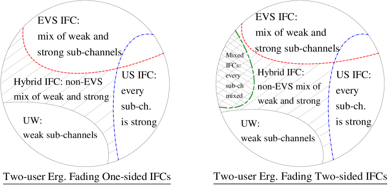
Figure 1: A Venn diagram representation of the four sub-classes of ergodic fading one- and two-sided IFCs.

II Channel Model and Preliminaries

Figure 2: The two-user Gaussian two-sided IFC and C-MAC and the two-user Gaussian one-sided IFC.

A two-sender two-receiver (also referred to as the two-user) ergodic fading Gaussian IFC consists of two source nodes $S_{1}$ and $S_{2}$, and two destination nodes $D_{1}$ and $D_{2}$ as shown in Fig. 2. Source $S_{k}$, $k=1,2$, uses the channel $n$ times to transmit its message $W_{k}$, which is distributed uniformly in the set $\,\{1,2,\ldots,2^{B_{k}}\}$ and is independent of the message from the other source, to its intended receiver, $D_{k}$, at a rate $R_{k}=B_{k}/n$ bits per channel use. In each use of the channel, $S_{k}$ transmits the signal $X_{k}$ while the destination $D_{k}$ receives $Y_{k}$, $k=1,2.$ For $\mathbf{X}=\left[X_{1}\text{ }X_{2}\right]^{T}$, the channel output vector $\mathbf{Y}=\left[Y_{1}\text{ }Y_{2}\right]^{T}$ is given by

$$\mathbf{Y}=\mathbf{HX}+\mathbf{Z}$$ (1)

where $\mathbf{Z}=\left[Z_{1}\text{ }Z_{2}\right]^{T}$ is a noise vector with entries that are zero-mean, unit variance, circularly symmetric complex Gaussian noise variables and $\mathbf{H}$ is a random matrix of fading gains with entries $H_{m,k}$, for all $m,k=1,2$, such that $H_{m,k}$ denotes the fading gain between receiver $m$ and transmitter $k$. We use $\mathbf{h}$ to denote a realization of $\mathbf{H}$. We assume the fading process $\left\{\mathbf{H}\right\}$ is stationary and ergodic but not necessarily Gaussian. Note that the channel gains $H_{m,k}$, for all $m$ and $k$, are not assumed to be independent; however, $\mathbf{H}$ is known instantaneously at all the transmitters and receivers.

Over $n$ uses of the channel, the transmit sequences $\left\{X_{k,i}\right\}$ are constrained in power according to

$$\left.\sum\limits_{i=1}^{n}\left|X_{k,i}\right|^{2}\leq n\overline{P}_{k}\right.,\text{ for all }k=1,2\text{.}$$ (2)

Since the transmitters know the fading states of the links on which they transmit, they can allocate their transmitted signal power according to the channel state information. A power policy $P$$(\mathbf{h})$ is a mapping from the fading state space consisting of the set of all fading states (instantiations) $\mathbf{h}$ to the set of non-negative real values in $\mathcal{R}_{+}^{2}$. The entries of $P$$(\mathbf{h})$ are $P_{k}(\mathbf{h})$, the power policy at user $k$, $k=1,2$. While $P$$(\mathbf{h})$ denotes the map for a particular fading state, we write $P$$(\mathbf{H})$ to explicitly describe the policy for the entire set of random fading states. Thus, we use the notation $P$$(\mathbf{H})$ when averaging over all fading states or describing a collection of policies, one for every $\mathbf{h}$. The entries of $P$$(\mathbf{H})$ are $P_{k}(\mathbf{H}),$ for all $k$.

For an ergodic fading channel, (2) then simplifies to

$$\left.\mathbb{E}\left[P_{k}(\mathbf{H})\right]\leq\overline{P}_{k}\right.\text{ for all }k=1,2,$$ (3)

where the expectation in (3) is over the distribution of $\mathbf{H}$. We denote the set of all feasible policies $\underline{P}\left(\mathbf{h}\right)$, i.e., the power policies whose entries satisfy (3), by $\mathcal{P}$. Finally, we write $\overline{P}$ to denote the vector of average power constraints with entries $\overline{P}_{k}$, $k=1,2$.

For the special case where both receivers decode the messages from both transmitters, we obtain a compound MAC (see Fig. 2(a)). A one-sided fading Gaussian IFC results when either $H_{1,2}=0$ or $H_{2,1}=0$ (see Fig. 2(b)). Without loss of generality, we develop sum-capacity results for a one-sided IFC (Z-IFC) with $H_{2,1}=0$. The results extend naturally to the complementary one-sided model with $H_{1,2}=0$. A two-sided IFC can be viewed as a collection of two complementary one-sided IFCs, one with $H_{1,2}=0$ and the other with $H_{2,1}=0$.

We write $\mathcal{C}_{\text{IFC}}\left(\overline{P}_{1},\overline{P}_{2}\right)$ and $\mathcal{C}_{\text{C-MAC}}\left(\overline{P}_{1},\overline{P}_{2}\right)$ to denote the capacity region of an ergodic fading IFC and C-MAC, respectively. Our definition of average error probabilities, capacity regions, and achievable rate pairs $\left(R_{1},R_{2}\right)$ for both the IFC and C-MAC mirror the standard information-theoretic definitions [29, Chap. 14].

Non-fading IFCs can be classified by the relative strengths of the interfering to intended signals at each of the receivers. A (two-sided non-fading) strong IFC is one in which the cross-link channel gains are larger than the direct link channel gains to the intended receivers [1], i.e.,

$$\begin{array}[c]{cc}\left|H_{j,k}\right|>\left|H_{k,k}\right|&\text{for all }j,k=1,2,\text{ }j\not=k.\end{array}$$ (4)

A strong IFC is very strong if the cross-link channel gains dominate the transmit powers such that (see for e.g., [1, 2])

$$\begin{array}[c]{cc}\sum\limits_{k=1}^{2}C\left(\left|H_{k,k}\right|^{2}P_{k}\left(\mathbf{H}\right)\right)<C\left(\sum\limits_{k=1}^{2}\left|H_{j,k}\right|^{2}P_{j}\left(\mathbf{H}\right)\right)&\text{for all }j=1,2,\end{array}$$ (5)

where for the non-fading IFC, $P_{k}\left(\mathbf{H}\right)=\overline{P}_{k}$ in (2). One can verify that (5) implies (4), i.e., a very strong IFC is also strong.

A non-fading IFC is weak when (4) is not satisfied for all $j,k$, i.e., neither of the two complementary one-sided IFCs that a two-sided IFC can be decomposed into are strong. A non-fading IFC is mixed when one of complementary one-sided IFCs is weak while the other is strong, i.e.,

$$\begin{array}[c]{ccc}\left|H_{1,2}\right|>\left|H_{2,2}\right|\text{ }&\text{and }&\left|H_{2,1}\right|<\left|H_{1,1}\right|\end{array}$$ (6)

or

$$\begin{array}[c]{ccc}\left|H_{1,2}\right|>\left|H_{2,2}\right|\text{ }&\text{and }&\left|H_{2,1}\right|<\left|H_{1,1}\right|.\end{array}$$ (7)

An ergodic fading IFC is a collection of parallel sub-channels (fading states), and thus, each sub-channel can be either very strong, strong, or weak. Since a fading IFC can contain a mixture of different types of sub-channels, we introduce the following definitions to classify the set of all ergodic fading two-user Gaussian IFCs (see also Fig. 1). Unless otherwise stated, we henceforth simply write IFC to denote a two-user ergodic fading Gaussian IFC.

Definition 1

A uniformly strong IFC is a collection of strong sub-channels, i.e., both cross-links in each sub-channel satisfy (4).

Definition 2

An ergodic very strong IFC is a collection of weak and strong (including very strong) sub-channels for which (5) is satisfied when averaged over all fading states and for $P_{k}\left(\mathbf{H}\right)=P_{k}^{\left(wf\right)}\left(H_{kk}\right)$, where $P_{k}^{\left(wf\right)}\left(H_{kk}\right)$ is the optimal waterfilling policy that achieves the point-to-point capacity for user $k$ in the absence of interference.

Definition 3

A uniformly weak IFC is a collection of weak sub-channels, i.e., in each sub-channel both cross-links do not satisfy (4).

Definition 4

A uniformly mixed IFC is a pair of two complementary one-sided IFCs in which one of them is uniformly weak and the other is uniformly strong.

Definition 5

A hybrid IFC is a collection of weak and strong sub-channels with at least one weak and one strong sub-channel that do not satisfy the conditions in (5) when averaged over all fading states and for $P_{k}\left(\mathbf{H}\right)=P_{k}^{\left(wf\right)}\left(H_{kk}\right)$.

Since an ergodic fading channel is a collection of parallel sub-channels (fading states) with different weights, throughout the sequel, we use the terms fading states and sub-channels interchangeably. In contrast to the one-sided IFC, we simply write IFC to denote the two-sided model. Before proceeding, we summarize the notation used in the sequel.

• Random variables (e.g. $H_{k,j}$) are denoted with uppercase letters and their realizations (e.g. $h_{k,j}$) with the corresponding lowercase letters.

• Bold font $\mathbf{X}$ denotes a random matrix while bold font $\mathbf{x}$ denotes an instantiation of $\mathbf{X}$.

• $I$ denotes the identity matrix.

• $\left|\mathbf{X}\right|$ and $\mathbf{X}^{-1}$ denotes the determinant and inverse of the matrix $\mathbf{X.}$

• $\mathcal{CN}\left(0,\mathbf{\Sigma}\right)$ denotes a circularly symmetric complex Gaussian distribution with zero mean and covariance $\mathbf{\Sigma}$.

• $\mathcal{K}=\left\{1,2\right\}$ denotes the set of transmitters.

• $\mathbb{E}\left(\cdot\right)$ denotes expectation; $C(x)$ denotes $\log(1+x)$ where the logarithm is to the base 2, $\left(x\right)^{+}$ denotes $\max(x,0)$, $I(\cdot;\cdot)$ denotes mutual information, $h\left(\cdot\right)$ denotes differential entropy, and $R_{\mathcal{S}}$ denotes ${\textstyle\sum\nolimits_{k\in\mathcal{S}}}R_{k}$ for any ${\mathcal{S}}$ $\subseteq\mathcal{K}$.

III Main Results

The following theorems summarize the main contributions of this paper. The proof for the capacity region of the C-MAC is presented in Section IV as are the details of determining the capacity achieving power policies. The proofs for the remaining theorems, related to IFCs, are collected in Section V. Throughout the sequel we write waterfilling solution to denote the capacity achieving power policy for ergodic fading point-to-point channels [19].

III-A Ergodic fading C-MAC

An achievable rate region for ergodic fading IFCs results from allowing both receivers to decode the messages from both transmitters, i.e., by converting an IFC to a C-MAC. The following theorem summarizes the sum-capacity $\mathcal{C}_{\text{C-MAC}}$ of an ergodic fading C-MAC.

Theorem 1

The capacity region, $\mathcal{C}_{\text{C-MAC}}\left(\overline{P}_{1},\overline{P}_{2}\right)$, of an ergodic fading two-user Gaussian C-MAC with average power constraints $P_{k}$ at transmitter $k$, $k=1,2,$ is

$$\mathcal{C}_{\text{C-MAC}}\left(\overline{P}_{1},\overline{P}_{2}\right)=\bigcup_{\underline{P}\in\mathcal{P}}\left\{\mathcal{C}_{1}\left(\underline{P}\left(\mathbf{H}\right)\right)\cap\mathcal{C}_{2}\left(\underline{P}\left(\mathbf{H}\right)\right)\right\}$$ (8)

where for $j=1,2,$ we have

$$\mathcal{C}_{j}\left(\underline{P}\left(\mathbf{H}\right)\right)=\left\{\left(R_{1},R_{2}\right):R_{\mathcal{S}}\leq\mathbb{E}\left[C\left(\sum_{k\in\mathcal{S}}\left|H_{j,k}\right|^{2}P_{k}\left(\mathbf{H}\right)\right)\right],\text{for all }\mathcal{S}\subseteq\mathcal{K}\right\}.$$ (9)

The optimal coding scheme requires encoding and decoding jointly across all sub-channels.

Remark 1

The capacity region $\mathcal{C}_{\text{C-MAC}}$ is convex. This follows from the convexity of the set $\mathcal{P}$ and the concavity of the $\log$ function.

Remark 2

$\mathcal{C}_{\text{C-MAC}}$ is a function of $\left(\overline{P}_{1},\overline{P}_{2}\right)$ due to the fact that union in (8) is over all feasible power policies, i.e., over all $\underline{P}\left(\mathbf{H}\right)$ whose entries satisfy (3).

Remark 3

In contrast to the ergodic fading point-to-point and multiple access channels, the ergodic fading C-MAC is not merely a collection of independent parallel channels; in fact encoding and decoding independently in each parallel channel is in general sub-optimal as demonstrated later in the sequel.

Corollary 1

The capacity region $\mathcal{C}_{\text{IFC}}$ of an ergodic fading IFC is bounded as $\mathcal{C}_{\text{C-MAC}}\subseteq\mathcal{C}_{\text{IFC}}$.

III-B Ergodic Very Strong IFCs

Theorem 2

The capacity region of an ergodic very strong IFC is

$$\mathcal{C}_{\text{IFC}}^{EVS}=\left\{\left(R_{1},R_{2}\right):R_{k}\leq\mathbb{E}\left[C\left(\left|H_{k,k}\right|^{2}P_{k}^{wf}\left(H_{k,k}\right)\right)\right],k=1,2\right\}.$$ (10)

The sum-capacity is

$$\sum_{k=1}^{2}\mathbb{E}\left[C\left(\left|H_{k,k}\right|^{2}P_{k}^{wf}\left(H_{k,k}\right)\right)\right]$$ (11)

where, for all $k,$ $P_{k}^{wf}\left(H_{j,k}\right)$ is the optimal waterfilling solution for an (interference-free) ergodic fading link between transmitter $k$ and receiver $k$ such that, $\underline{P}^{wf}\left(H_{k,k}\right)$ satisfies

$$\sum_{k=1}^{2}\mathbb{E}\left[C\left(\left|H_{k,k}\right|^{2}P_{k}^{wf}\left(H_{k,k}\right)\right)\right]<\min_{j=1,2}\mathbb{E}\left[C\left(\sum_{k=1}^{2}\left|H_{j,k}\right|^{2}P_{k}^{wf}\left(H_{k,k}\right)\right)\right].$$ (12)

The capacity achieving scheme requires encoding and decoding jointly across all sub-channels at the transmitters and receivers respectively. The optimal strategy also requires both receivers to decode messages from both transmitters.

Remark 4

In the sequel we show that the condition in (12) is a result of the achievable strategy, and therefore is a sufficient condition. For the special case of fixed (non-fading) channel gains $\mathbf{H}$, and $P_{k}^{\ast}=\overline{P}_{1}$, (12) reduces to the general conditions for a very strong IFC (see for e.g., [1]) given by

$$\left|H_{1,2}\right|^{2} >\left|H_{2,2}\right|^{2}\left(1+\left|H_{1,1}\right|^{2}\overline{P}_{1}\right)$$ (13a)

$$\left|H_{2,1}\right|^{2} >\left|H_{1,1}\right|^{2}\left(1+\left|H_{2,2}\right|^{2}\overline{P}_{2}\right).$$ (13b)

In contrast, the fading averaged conditions in (12) imply that not every sub-channel needs to satisfy (13) and in fact, the ergodic very strong channel can be a mix of weak and strong channels provided $$\underline{P}^{\left(wf\right)}$$ satisfies (12). This in turn implies that not every parallel sub-channel needs to be a strong (non-fading) Gaussian IFC.

Remark 5

The set of strong fading IFCs for which every sub-channel is strong and the optimal waterfilling policies for the two interference-free links satisfy (12) is strictly a subset of the set of ergodic very strong IFCs.

Remark 6

As stated in Theorem 2, the capacity achieving scheme for EVS IFCs requires coding jointly across all sub-channels. Coding independent messages (separable coding) across the sub-channels is optimal only when every sub-channel is very strong at the optimal policy $\underline{P}^{\left(wf\right)}$.

III-C Uniformly Strong IFC

In the following theorem, we present the capacity region and the sum-capacity of a uniformly strong IFC.

Theorem 3

The capacity region of a uniformly strong fading IFC for which the entries of every fading state $\mathbf{h}$ satisfy

$$\begin{array}[c]{ccc}\left|h_{1,1}\right|\leq\left|h_{2,1}\right|&\text{and}&\left|h_{2,2}\right|\leq\left|h_{1,2}\right|\end{array}$$ (14)

is given by

$$\mathcal{C}_{\text{IFC}}^{US}\left(\overline{P}_{1},\overline{P}_{2}\right)=\mathcal{C}_{\text{C-MAC}}\left(\overline{P}_{1},\overline{P}_{2}\right)$$ (15)

where $\mathcal{C}_{\text{C-MAC}}\left(\overline{P}_{1},\overline{P}_{2}\right)$ is the capacity of an ergodic fading C-MAC with the same channel statistics as the IFC. The sum-capacity is

$$\max_{\underline{P}\left(\mathbf{H}\right)\in\mathcal{P}}\min\left\{\min_{j=1,2}\left\{\mathbb{E}\left[C\left({\textstyle\sum\nolimits_{k=1}^{2}}\left|H_{j,k}\right|^{2}P_{k}\left(\mathbf{H}\right)\right)\right]\right\},\sum_{k=1}^{2}\mathbb{E}\left[C\left(\left|H_{k,k}\right|^{2}P_{k}\left(\mathbf{H}\right)\right)\right]\right\}.$$ (16)

The capacity achieving scheme requires encoding and decoding jointly across all sub-channels at the transmitters and receivers, respectively, and also requires both receivers to decode messages from both transmitters.

Remark 7

In contrast to the very strong case, every sub-channel in a uniformly strong fading IFC is strong.

Remark 8

The uniformly strong condition may suggest that separability is optimal. However, the capacity achieving C-MAC approach requires joint encoding and decoding across all sub-channels. A strategy where each sub-channel is viewed as an independent IFC, as in [14], will in general be strictly sub-optimal. This is seen directly from comparing (16) with the sum-rate achieved by coding independently over the sub-channels which is given by

$$\max_{\underline{P}\left(\mathbf{H}\right)\in\mathcal{P}}\mathbb{E}\left\{\min\left\{\min_{j=1,2}\left\{C\left({\textstyle\sum\nolimits_{k=1}^{2}}\left|H_{j,k}\right|^{2}P_{k}\left(\mathbf{H}\right)\right)\right\}\right.\right.,\left.\left.\sum_{k=1}^{2}C\left(\left|H_{k,k}\right|^{2}P_{k}\left(\mathbf{H}\right)\right)\right\}\right\}.\text{ \ \ \ \ \ \ \ \ \ \ }$$ (17)

The sub-optimality of independent encoding follows directly from the fact that for two random variables $A\left(\mathbf{H}\right)$ and $\not B\left(\mathbf{H}\right),$ $\mathbb{E}[\min\left(A\left(\mathbf{H}\right),B\left(\mathbf{H}\right)\right)]$ $\leq$ $\min\left(\mathbb{E}[A\left(\mathbf{H}\right)],\mathbb{E}[B\left(\mathbf{H}\right)]\right)]$ with equality if and only if for every fading instantiation $\mathbf{h}$, $A\left(\mathbf{H}\right)$ (resp. $B\left(\mathbf{H}\right)$) dominates $B\left(\mathbf{H}\right)$ (resp. $A\left(\mathbf{H}\right)$). Thus, independent (separable) encoding across sub-channels is optimal only when, at $\underline{P}^{\ast}\left(\mathbf{H}\right)$, the sum-rate in every sub-channel in (17) is maximized by the same sum-rate function.

III-D Uniformly Weak One-Sided IFC

The following theorem summarizes the sum-capacity of a one-sided uniformly weak IFC in which every sub-channel is weak.

Theorem 4

The sum-capacity of a uniformly weak ergodic fading Gaussian one-sided IFC for which the entries of every fading state $\underline{h}$ satisfy

$$\begin{array}[c]{c}\left|h_{2,2}\right|>\left|h_{1,2}\right|\end{array}$$ (18)

is given by

$$\max_{\underline{P}\left(\mathbf{H}\right)\in\mathcal{P}}\left\{S^{\left(w,1\right)}\left(\underline{P}\left(\mathbf{H}\right)\right)\right\}$$ (19)

where

$$S^{\left(w,1\right)}\left(\underline{P}\left(\mathbf{H}\right)\right)=\mathbb{E}\left[C\left(\frac{\left|H_{1,1}\right|^{2}P_{1}\left(\mathbf{H}\right)}{1+\left|H_{1,2}\right|^{2}P_{2}\left(\mathbf{H}\right)}\right)+C\left(\left|H_{2,2}\right|^{2}P_{2}\left(\mathbf{H}\right)\right)\right].$$ (20)

Remark 9

One could alternately consider the fading one-sided IFC in which $\left|h_{1,1}\right|>\left|h_{2,1}\right|$ and $h_{1,2}=0$ for the sum-capacity is given by (19) with the superscript $1$ replaced by 2. The expression $S^{\left(w,2\right)}\left(\underline{P}\left(\mathbf{H}\right)\right)$ is given by (20) after swapping the indexes $1$ and $2$.

III-E Uniformly Mixed IFC

The following theorem summarizes the sum-capacity of a class of uniformly mixed two-sided IFC.

Theorem 5

For a class of uniformly mixed ergodic fading two-sided Gaussian IFCs for which the entries of every fading state $\underline{h}$ satisfy

$$\begin{array}[c]{ccc}\left|h_{1,1}\right|>\left|h_{2,1}\right|&\text{and}&\left|h_{2,2}\right|\leq\left|h_{1,2}\right|\end{array}$$ (21)

the sum-capacity is

$$\max_{\underline{P}\left(\mathbf{H}\right)\in\mathcal{P}}\left\{\min\left(\mathbb{E}\left[C\left({\textstyle\sum\nolimits_{k=1}^{2}}\left|H_{1,k}\right|^{2}P_{k}\left(\mathbf{H}\right)\right)\right],S^{\left(w,2\right)}\left(\underline{P}\left(\mathbf{H}\right)\right)\right)\right\}$$ (22)

where $S^{\left(w,2\right)}\left(\underline{P}\left(\mathbf{H}\right)\right)$ is given by (20) by swapping indexes $1$ and $2$.

Remark 10

One could alternately consider the fading IFC in which $\left|h_{1,1}\right|\leq\left|h_{2,1}\right|$ and $\left|h_{2,2}\right|>\left|h_{1,2}\right|$. The sum-capacity is given by (22) after swapping the indexes $1$ and $2$.

Remark 11

For the special case of $H_{k,k}=\sqrt{SNR}e^{j\phi_{kk}}$ and $H_{j,k}=\sqrt{INR}e^{j\phi_{jk}}$, $j\not=k$, where $\phi_{j,k}$ for all $j$ and $k$ is independent and distributed uniformly in $\left[-\pi,\pi\right]$, the sum-capacity in Theorems 3 and 5 can also be achieved by ergodic interference alignment as shown in [25].

III-F Uniformly Weak IFC

The sum-capacity of a one-sided uniformly weak IFC in Theorem 4 is an upper bound for that of a two-sided IFC for which at least one of two one-sided IFCs that result from eliminating a cross-link is uniformly weak. Similarly, a bound can be obtained from the sum-capacity of the complementary one-sided IFC. The following theorem summarizes this result.

Theorem 6

For a class of uniformly weak ergodic fading two-sided Gaussian IFCs for which the entries of every fading state $\underline{h}$ satisfy

$$\begin{array}[c]{ccc}\left|h_{1,1}\right|>\left|h_{2,1}\right|&\text{and}&\left|h_{2,2}\right|>\left|h_{1,2}\right|\end{array}$$ (23)

the sum-capacity is upper bounded as

$$R_{1}+R_{2}\leq\max_{\underline{P}\left(\mathbf{H}\right)\in\mathcal{P}}\min\left(S^{\left(w,1\right)}\left(\underline{P}\left(\mathbf{H}\right)\right),S^{\left(w,2\right)}\left(\underline{P}\left(\mathbf{H}\right)\right)\right).$$ (24)

Remark 12

For the non-fading case, the sum-rate bounds in (24) simplify to those obtained in [9, Theorem 3].

III-G One-sided IFC: General Achievable Scheme

For EVS and US IFCs, Theorems 2 and 3 suggest that joint coding across all sub-channels is optimal. Particularly for EVS, such joint coding allows one to exploit the strong states in decoding messages. Relying on this observation, we present an achievable strategy based on joint coding all sub-classes of one-sided IFCs with $H_{2,1}=0$. The encoding scheme involves rate-splitting at user $2$, i.e., user $2$ transmits $w_{2}=\left(w_{2p},w_{2c}\right)$ where $w_{2p}$ and $w_{2c}$ are private and common messages, respectively and can be viewed as a Han-Kobayashi scheme with Gaussian codebooks and without time-sharing.

Theorem 7

The sum-capacity of a one-sided IFC is lower bounded by

$$\max_{\underline{P}\left(\mathbf{H}\right)\in\mathcal{P},\alpha_{\mathbf{H}}\in[0,1]}\min\left(S_{1}\left(\alpha_{\mathbf{H}},\underline{P}\left(\mathbf{H}\right)\right),S_{2}\left(\alpha_{\mathbf{H}},\underline{P}\left(\mathbf{H}\right)\right)\right)$$ (25)

where

$$S_{1}\left(\alpha_{\mathbf{H}},\underline{P}\left(\mathbf{H}\right)\right) =\mathbb{E}\left[C\left(\frac{\left|H_{1,1}\right|^{2}P_{1}\left(\mathbf{H}\right)}{1+\left|H_{1,2}\right|^{2}\alpha_{\mathbf{H}}P_{2}\left(\mathbf{H}\right)}\right)\right]+\mathbb{E}\left[C\left(\left|H_{2,2}\right|^{2}P_{2}\left(\mathbf{H}\right)\right)\right],$$ (26)

$$S_{2}\left(\alpha_{\mathbf{H}},\underline{P}\left(\mathbf{H}\right)\right) =\mathbb{E}\left[C\left(\left|H_{2,2}\right|^{2}\alpha_{\mathbf{H}}P_{2}\left(\mathbf{H}\right)\right)\right]+\mathbb{E}\left[C\left(\frac{\left|H_{1,1}\right|^{2}P_{1}\left(\mathbf{H}\right)+\left|H_{1,2}\right|^{2}\overline{\alpha}_{\mathbf{H}}P_{2}\left(\mathbf{H}\right)}{1+\left|H_{1,2}\right|^{2}\alpha_{\mathbf{H}}P_{2}\left(\mathbf{H}\right)}\right)\right],$$ (27)

such that $\alpha_{\mathbf{H}}$ is the power allocated by user $2$ in fading state $\mathbf{H}$ to transmitting $w_{2p}$ and $\overline{\alpha}_{\mathbf{H}}=1-\alpha_{\mathbf{H}}$, $\alpha_{\mathbf{H}}\in\left[0,1\right]$. For EVS one-sided IFCs, the sum-capacity is achieved by choosing $\alpha_{\mathbf{H}}=0$ for all $\mathbf{H}$ provided $S_{1}\left(0,\underline{P}^{(wf)}\left(\mathbf{H}\right)\right)<S_{2}\left(0,\underline{P}^{(wf)}\left(\mathbf{H}\right)\right)$. For US one-sided IFCs, the sum-capacity is given by (25) for $\alpha_{\mathbf{H}}=0$ for all $\mathbf{H}$. For UW one-sided IFCs, the sum-capacity is achieved by choosing $\alpha_{\mathbf{H}}=1$ and maximizing $S_{2}\left(1,\underline{P}\left(\mathbf{H}\right)\right)=S_{1}\left(1,\underline{P}\left(\mathbf{H}\right)\right)$ over all feasible $\underline{P}\left(\mathbf{H}\right).$ For a hybrid one-sided IFC, the achievable sum-rate is maximized by

$$\alpha_{\mathbf{H}}^{\ast}=\left\{\begin{array}[c]{cc}\alpha\left(\mathbf{H}\right)\in(0,1]&\text{sub-channel }\mathbf{H}\text{ is weak }\\ 0&\text{sub-channel }\mathbf{H}\text{ is strong.}\end{array}\right.$$ (28)

and is given by (25) for this choice of $\alpha_{\mathbf{H}}^{\ast}$.

Remark 13

The optimal $\alpha_{\mathbf{H}}^{\ast}$ in (28) implies that in general for the hybrid one-sided IFCs joint coding the transmitted message across all sub-channels is optimal. Specifically, the common message is transmitted jointly in all sub-channels while the private message is transmitted only in the weak sub-channels.

Remark 14

The separation-based coding scheme of [30] is a special case of the above HK-based coding scheme and is obtained by choosing $\alpha_{\mathbf{H}}=1$ and $\alpha_{\mathbf{H}}=0$ for the weak and strong states, respectively. The resulting sum-rate is at most as large as the bound in (25) obtained for $\alpha_{\mathbf{H}}^{\ast}\in(0,1]$ and $\alpha_{\mathbf{H}}^{\ast}=0$ for the weak and strong states, respectively.

Remark 15

In [26], a Han-Kobayashi based scheme using Gaussian codebooks and no time-sharing is used to develop an inner bound on the capacity region of a two-sided IFC.

IV Compound MAC: Capacity Region and Optimal Policies

As stated in Corollary 1, an inner bound on the sum-capacity of an IFC can be obtained by allowing both receivers to decode both messages, i.e., by determining the sum-capacity of a C-MAC with the same inter-node links. In this Section, we prove Theorem 1 which establishes the capacity region of ergodic fading C-MACs and discuss the optimal power policies that achieve every point on the boundary of the capacity region.

IV-A Capacity Region

The capacity region of a discrete memoryless compound MAC is developed in [31]. For each choice of input distribution at the two independent sources, this capacity region is an intersection of the MAC capacity regions achieved at the two receivers. The techniques in [31] can be easily extended to develop the capacity region for a Gaussian C-MAC with fixed channel gains. For the Gaussian C-MAC, one can show that Gaussian signaling achieves the capacity region using the fact that Gaussian signaling maximizes the MAC region at each receiver. Thus, the Gaussian C-MAC capacity region is an intersection of the Gaussian MAC capacity regions achieved at $D_{1}$ and $D_{2}$. For a stationary and ergodic process $\left\{\mathbf{H}\right\}$, the channel in (1) can be modeled as a parallel Gaussian C-MACs consisting of a collection of independent Gaussian C-MACs, one for each fading state $\mathbf{h}$, with an average transmit power constraint over all parallel channels.

We now prove Theorem 1 stated in Section III-A which gives the capacity region of ergodic fading C-MACs.

Proof of Theorem 1

We first present an achievable scheme. Consider a policy $\underline{P}\left(\mathbf{H}\right)\in\mathcal{P}$. The achievable scheme involves requiring each transmitter to encode the same message across all sub-channels and each receiver to jointly decode over all sub-channels. Independent codebooks are used for every sub-channel. An error occurs at receiver $j$ if one or both messages decoded jointly across all sub-channels is different from the transmitted message. Given this encoding and decoding, the analysis at each receiver mirrors that for a MAC receiver [29, 14.3] and one can easily verify that for reliable reception of the transmitted message at receiver $j$, the rate pair $\left(R_{1},R_{2}\right)$ needs to satisfy the rate constraints in (9) where in decoding $w_{\mathcal{S}}=\left\{w_{k}:k\in\mathcal{S}\right\}$ the information collected in each sub-channel is given by $C\left(\sum_{k\in\mathcal{S}}\left|H_{j,k}\right|^{2}P_{k}\left(\mathbf{H}\right)\right)$, for all $\mathcal{S}\subseteq\mathcal{K}.$ Thus, for any feasible $\underline{P}\left(\mathbf{H}\right)$, the achievable rate region is given by $\mathcal{C}_{1}\left(\underline{P}\left(\mathbf{H}\right)\right)\cap\mathcal{C}_{2}\left(\underline{P}\left(\mathbf{H}\right)\right)$. From the concavity of the $\log$ function, the achievable region over all $\underline{P}\left(\mathbf{H}\right)$ is given by (8).
  For the converse, the proof technique mirrors the proof for the capacity of an ergodic fading MAC developed in [20, Appendix A]. For any $\underline{P}\left(\mathbf{H}\right)\in\mathcal{P}$, one can using similar limiting arguments to show that for asymptotically error-free performance at receiver $j$, for all $j$, the achievable region has to be bounded as

$$\begin{array}[c]{cc}R_{\mathcal{S}}\leq\mathbb{E}\left[C\left(\sum_{k\in\mathcal{S}}\left|H_{j,k}\right|^{2}P_{k}\left(\mathbf{H}\right)\right)\right],&j=1,2.\end{array}$$ (29)

The proof is completed by noting that due to the concavity of the $\log$ it suffices to take the union of the region over all $\underline{P}\left(\mathbf{H}\right)\in\mathcal{P}$.

Remark 16

An achievable scheme in which independent messages are encoded in each sub-channel, i.e., separable coding, will in general not achieve the capacity region. This is due to the fact that for this separable coding scheme the achievable rate in each sub-channel is a minimum of the rates at each receiver. The average of such minima can at most be the minimum of the average rates at each receiver, where the latter is achieved by encoding the same message jointly across all sub-channels.

Corollary 1 follows from the argument that a rate pair in $\mathcal{C}_{\text{C-MAC}}$ is achievable for the IFC since $\mathcal{C}_{\text{C-MAC}}$ is the capacity region when both messages are decoded at both receivers.

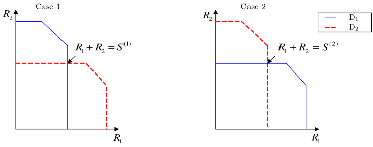
Figure 3: Rate regions $\mathcal{C}_{1}(\underline{P}(\underline{H}))$ and $\mathcal{C}_{2}(\underline{P}(\underline{H}))$ and sum-rate for case 1 and case 2.

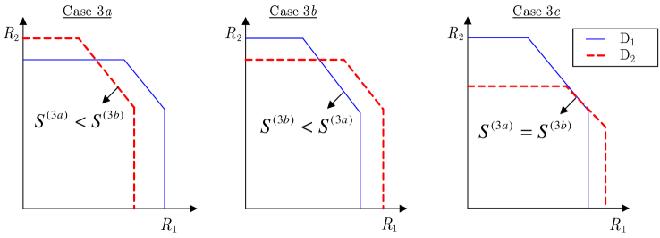
Figure 4: Rate regions $R_{r}(\underline{P}(\underline{H}))$ and $R_{d}(\underline{P}(\underline{H}))$ and sum-rate for cases $3a$, $3b$, and $3c$.

IV-B Sum-Capacity Optimal Policies

The capacity region $\mathcal{C}_{\text{C-MAC}}$ is a union of the intersection of the pentagons $\mathcal{C}_{1}\left(\underline{P}\left(\mathbf{H}\right)\right)$ and $\mathcal{C}_{2}\left(\underline{P}\left(\mathbf{H}\right)\right)$ achieved at $D_{1}$ and $D_{2},$ respectively, where the union is over all $\underline{P}\left(\mathbf{H}\right)\in\mathcal{P}$. The region $\mathcal{C}_{\text{C-MAC}}$ is convex, and thus, each point on the boundary of $\mathcal{C}_{\text{C-MAC}}$ is obtained by maximizing the weighted sum $\mu_{1}R_{1}$ $+$ $\mu_{2}R_{2}$ over all $\underline{P}\left(\mathbf{H}\right)\in\mathcal{P}$, and for all $\mu_{1}>0$, $\mu_{2}>0$, subject to (29). In this section, we determine the optimal policy $\underline{P}^{\ast}\left(\mathbf{H}\right)$ that maximizes the sum-rate $R_{1}+R_{2}$ when $\mu_{1}$ $=$ $\mu_{2}$ $=$ $1$. Using the fact that the rate regions $\mathcal{C}_{1}\left(\underline{P}\left(\mathbf{H}\right)\right)$ and $\mathcal{C}_{2}\left(\underline{P}\left(\mathbf{H}\right)\right)$, for any feasible $\underline{P}\left(\mathbf{H}\right)$, are pentagons, in Figs. 3 and 4 we illustrate the five possible choices for the sum-rate resulting from an intersection of $\mathcal{C}_{1}\left(\underline{P}\left(\mathbf{H}\right)\right)$ and $\mathcal{C}_{2}\left(\underline{P}\left(\mathbf{H}\right)\right)$ (see also [32]).

Cases $1$ and $2$, as shown in Fig. 3 and henceforth referred to as inactive cases, are such that the constraints on the two sum-rates are not active in $\mathcal{C}_{1}\left(\underline{P}\left(\mathbf{H}\right)\right)\cap\mathcal{C}_{2}\left(\underline{P}\left(\mathbf{H}\right)\right)$, i.e., no rate tuple on the sum-rate plane achieved at one of the receivers lies within or on the boundary of the rate region achieved at the other receiver. In contrast, when there exists at least one such rate tuple such that the two sum-rates constraints are active in $\mathcal{C}_{1}\left(\underline{P}\left(\mathbf{H}\right)\right)\cap\mathcal{C}_{2}\left(\underline{P}\left(\mathbf{H}\right)\right)$ are the active cases. This includes Cases $3a$, $3b$, and $3c$ shown in Fig. 4 where the sum-rate at $D_{1}$ is smaller, larger, or equal, respectively, to that achieved at $D_{2}$. By definition, the active set also include the boundary cases in which there is exactly one rate pair that lies within or on the boundary of the rate region achieved at the other receiver. There are six possible boundary cases that lie at the intersection of an inactive case $l$, $l=1,2,$ and an active case $n,$ $n=3a,3b,3c$. There are six such boundary cases that we denote as cases $\left(l,n\right)$, $l=1,2,$ and $n=3a,3b,3c$.

In general, it is not possible to know a priori the type of intersection that will maximize the sum-capacity. Thus, the sum-rate for each case has to be maximized over all $\underline{P}\left(\mathbf{H}\right)\in\mathcal{P}$. To simplify optimization and obtain a unique solution, we explicitly consider the six boundary cases as distinct from the active cases thereby ensuring that the subsets of power policies resulting in the different cases are disjoint, i.e., no power policy results in more than one case. This in turn implies that the power policies resulting in each case satisfy specific conditions that distinguish that case from all others. For example, from Fig. 3, Case 1 results only when $\sum\nolimits_{k=1}^{2}C\left(H_{kk}P_{k}^{\left(wf\right)}\left(\mathbf{H}\right)\right)<C\left(\sum\nolimits_{k=1}^{2}H_{j,k}P_{k}^{\left(wf\right)}\left(\mathbf{H}\right)\right)$, for all $j=1,2.$ Using these disjoint cases and the fact that the rate expressions in (29) are concave functions of $\underline{P}\left(\mathbf{H}\right)$ allows us to develop closed form sum-capacity results and optimal policies for all cases. Observe that cases $1$ and $2$ do not share a boundary since such a transition (see Fig. 3) requires passing through case $3a$ or $3b$ or $3c$. Finally, note that Fig. 4 illustrates two specific $\mathcal{C}_{1}$ and $\mathcal{C}_{2}$ regions for $3a$, $3b$, and $3c$. The conditions for each case are shown in Figs. 3-6.

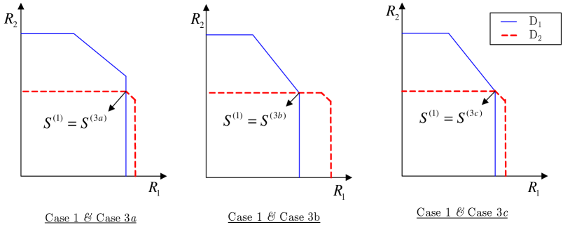
Figure 5: Rate regions $R_{r}(\underline{P}(\underline{H}))$ and $R_{d}(\underline{P}(\underline{H}))$ for cases (1,3a), (1,3b), and (1,3c).

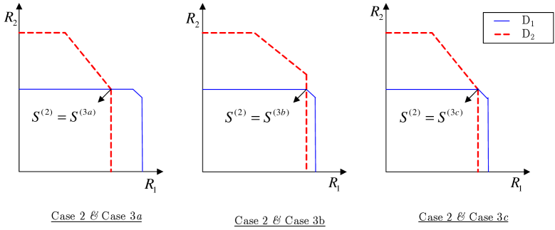
Figure 6: Rate regions $R_{r}(\underline{P}(\underline{H}))$ and $R_{d}(\underline{P}(\underline{H}))$ for cases (2,3a), (2,3b), and (2,3c).

Let $\underline{P}^{(i)}(\mathbf{H})$ and $\underline{P}^{(l,n)}(\mathbf{H})$ denote the optimal policies for cases $i$ and $(l,n)$, respectively. Let $S^{\left(i\right)}(\underline{P}(\mathbf{H}))$ and $S^{\left(l,n\right)}(\underline{P}(\mathbf{H}))$ denote the sum-rate achieved for cases $i$ and $\left(l,n\right)$, respectively, for some $\underline{P}(\mathbf{H})\in\mathcal{P}$. The optimization problem for case $i$ or case $\left(l,n\right)$ is given by

$$\begin{array}[c]{l}\max\limits_{\underline{P}\left(\mathbf{H}\right)\in\mathcal{P}}S^{\left(i\right)}\left(\underline{P}\left(\mathbf{H}\right)\right)\text{ or }\max\limits_{\underline{P}\left(\mathbf{H}\right)\in\mathcal{P}}S^{\left(l,n\right)}\left(\underline{P}\left(\mathbf{H}\right)\right)\\ \begin{array}[c]{ccc}s.t.&\mathbb{E}\left[P_{k}(\mathbf{H})\right]\leq\overline{P}_{k}\text{,}&\text{ }k=1,2,\end{array}\\ \begin{array}[c]{ccc}\text{ \ \ \ \ \ }&P_{k}(\mathbf{H})\geq 0\text{,}&\text{ }k=1,2,\text{ for all }\mathbf{H}\end{array}\end{array}$$ (30)

where

$$\begin{array}[c]{l}\begin{array}[c]{cc}S^{\left(1\right)}\left(\underline{P}\left(\mathbf{H}\right)\right)=\sum_{k=1}^{2}\mathbb{E}\left[C\left(\left|H_{k,k}\right|^{2}P_{k}\left(\mathbf{H}\right)\right)\right]&\end{array}\\ \begin{array}[c]{cc}S^{\left(2\right)}\left(\underline{P}\left(\mathbf{H}\right)\right)=\sum_{k=1}^{2}\mathbb{E}\left[C\left(\left|H_{j,k}\right|^{2}P_{k}\left(\mathbf{H}\right)\right)\right],&j,k=1,2\text{, }j\not=k\end{array}\\ \begin{array}[c]{cc}S^{\left(i\right)}\left(\underline{P}\left(\mathbf{H}\right)\right)=\mathbb{E}\left[C\left(\sum_{k=1}^{2}\left|H_{j,k}\right|^{2}P_{k}\left(\mathbf{H}\right)\right)\right],&\text{ for }\left(i,j\right)=\left(3a,2\right),\left(3b,1\right)\end{array}\\ \begin{array}[c]{cc}S^{\left(3c\right)}\left(\underline{P}\left(\mathbf{H}\right)\right)=S^{\left(3a\right)}\left(\underline{P}\left(\mathbf{H}\right)\right),&\text{ }s.t.\text{ }S^{\left(3a\right)}\left(\underline{P}\left(\mathbf{H}\right)\right)=S^{\left(3b\right)}\left(\underline{P}\left(\mathbf{H}\right)\right)\end{array}\text{ }\\ \begin{array}[c]{ccc}S^{\left(l,n\right)}\left(\underline{P}\left(\mathbf{H}\right)\right)=S^{\left(l\right)}\left(\underline{P}\left(\mathbf{H}\right)\right),&\text{ }s.t.\text{ }S^{\left(l\right)}\left(\underline{P}\left(\mathbf{H}\right)\right)=S^{\left(n\right)}\left(\underline{P}\left(\mathbf{H}\right)\right).&\text{for all }\left(l,n\right).\end{array}\end{array}$$ (31)

The conditions for each case are (see Figs 3-6) given below where for each case the condition holds true when evaluated at the optimal policies $\underline{P}^{\left(i\right)}(\mathbf{H})$ and $\underline{P}^{\left(l,n\right)}(\mathbf{H})$ for cases $i$ and $\left(l,n\right)$, respectively. For ease of notation, we do not explicitly denote the dependence of $S^{\left(i\right)}$ and $S^{\left(l,n\right)}$ on the appropriate $\underline{P}^{\left(i\right)}(\mathbf{H})$ and $\underline{P}^{\left(l,n\right)}(\mathbf{H})$, respectively.

$$\begin{array}[c]{cl}\underline{\text{Case}\ 1}:&S^{\left(1\right)}<\min\left(S^{\left(3a\right)},S^{\left(3b\right)}\right)\end{array}$$ (33)

$$\begin{array}[c]{cl}\underline{\text{Case}\ 2}:&S^{\left(2\right)}<\min\left(S^{\left(3a\right)},S^{\left(3b\right)}\right)\end{array}$$ (35)

$$\begin{array}[c]{cc}\underline{\text{Case}\ 3a}:&S^{\left(3a\right)}<\min\left(S^{\left(3b\right)},S^{\left(1\right)},S^{\left(2\right)}\right)\end{array}$$ (37)

$$\begin{array}[c]{cc}\underline{\text{Case}\ 3b}:&S^{\left(3b\right)}<\min\left(S^{\left(3a\right)},S^{\left(1\right)},S^{\left(2\right)}\right)\end{array}$$ (39)

$$\begin{array}[c]{cc}\underline{\text{Case}\ 3c}:&S^{\left(3a\right)}=S^{\left(3b\right)}<\min\left(S^{\left(1\right)},S^{\left(2\right)}\right)\end{array}$$ (41)

$$\begin{array}[c]{cccc}\underline{\text{Case}\ \left(1,3a\right)}:&S^{\left(3a\right)}<S^{\left(3b\right)}&\text{and}&S^{\left(1\right)}<S^{\left(3b\right)}\end{array}$$ (43)

$$\begin{array}[c]{cccc}\underline{\text{Case}\ \left(2,3a\right)}:&S^{\left(3a\right)}<S^{\left(3b\right)}&\text{and}&S^{\left(2\right)}<S^{\left(3b\right)}\end{array}$$ (45)

$$\begin{array}[c]{cccc}\underline{\text{Case}\ \left(1,3b\right)}:&S^{\left(3b\right)}<S^{\left(3a\right)}&\text{and}&S^{\left(1\right)}<S^{\left(3a\right)}\end{array}$$ (47)

$$\begin{array}[c]{cccc}\underline{\text{Case}\ \left(2,3b\right)}:&S^{\left(3b\right)}<S^{\left(3a\right)}&\text{and}&S^{\left(2\right)}<S^{\left(3a\right)}\end{array}$$ (49)

$$\begin{array}[c]{cc}\underline{\text{Case}\ \left(1,3c\right)}:&S^{\left(3a\right)}=S^{\left(3b\right)}=S^{\left(1\right)}<S^{\left(2\right)}\end{array}$$ (51)

$$\begin{array}[c]{cc}\underline{\text{Case}\ \left(2,3c\right)}:&S^{\left(3a\right)}=S^{\left(3b\right)}=S^{\left(2\right)}<S^{\left(1\right)}.\end{array}$$ (53)

The optimal policy for each case is determined using Lagrange multipliers and the Karush-Kuhn-Tucker (KKT) conditions. The sum-capacity optimal $P$${}^{\ast}\left(\mathbf{H}\right)$ is given by that $\underline{P}^{(i)}\left(\mathbf{H}\right)$ or $\underline{P}^{(l,n)}\left(\mathbf{H}\right)$ that satisfies the conditions of its case in (33)-(53).

Remark 17

For cases $1$ and $2$, one can expand the capacity expressions to verify that the conditions $S^{\left(l\right)}<\min\left(S^{\left(3a\right)},S^{\left(3b\right)}\right)$, $l=1,2,$ imply that $S^{\left(1\right)}<S^{\left(2\right)}$ and vice-versa. Therefore, if the optimal policy is determined in the order of the cases in (33)-(53), the conditions for cases $\left(1,3c\right)$ and $\left(2,3c\right)$ are tested only after all other cases have been excluded. Furthermore, the two cases are mutually exclusive, and thus, (51) and (53) simply redundant conditions written for completeness.

Remark 18

For the two-user case the conditions can be written directly from the geometry of intersecting rate regions for each case. However, for a more general $K$-user C-MAC, the conditions can be written using the fact that the rate regions for any $\underline{P}\left(\mathbf{H}\right)$ are polymatroids and that the sum-rate of two intersecting polymatroids is given by the polymatroid intersection lemma. A detailed analysis of the rate-region and the optimal policies using the polymatroid intersection lemma for a $K$-user two-receiver network is developed in [33].

The following theorem summarizes the form of $P$${}^{\ast}\left(\mathbf{H}\right)$ and presents an algorithm to compute it. The optimal policy maximizing each case can be obtained in a straightforward manner using standard constrained convex maximization techniques. The algorithm exploits the fact that each the occurence of one case excludes all other cases and the case that occurs is the one for which the optimal policy satisfies the case conditions. We refer the reader to [33, Appendix] for a detailed analysis.

Theorem 8

The optimal policy $\underline{P}^{\ast}\left(\mathbf{H}\right)$ achieving the sum-capacity of a two-user ergodic fading C-MAC is obtained by computing $\underline{P}^{(i)}\left(\mathbf{H}\right)$ and $\underline{P}^{(l,n)}\left(\mathbf{H}\right)$ starting with cases $1$ and $2$, followed by cases $3a,$ $3b,$ and $3c$, in that order, and finally the boundary cases $(l,n),$ in the order that cases $\left(l,3c\right)$ are the last to be optimized, until for some case the corresponding $\underline{P}^{(i)}\left(\mathbf{H}\right)$ or $\underline{P}^{(l,n)}\left(\mathbf{H}\right)$ satisfies the case conditions. The optimal $P$${}^{\ast}\left(\mathbf{H}\right)$ is given by the optimal $\underline{P}^{(i)}\left(\mathbf{H}\right)$ or $\underline{P}^{(l,n)}\left(\mathbf{H}\right)$ that satisfies its case conditions and falls into one of the following three categories:

Cases $1$ and $2$: The optimal policies for the two users are such that each user water-fills over its bottle-neck link, i.e., over the direct link to that receiver with the smaller (interference-free) ergodic fading capacity. Thus for cases $1$ and $2$, each transmitter water-fills on the (interference-free) point-to-point links to its intended and unintended receivers, respectively. Thus, for case $1$, $P_{k}^{\left(\ast\right)}\left(\mathbf{H}\right)=P_{k}^{\left(1\right)}\left(\mathbf{H}\right)=P_{k}^{wf}\left(H_{k,k}\right)$, and for case 2, $P_{k}^{\left(\ast\right)}\left(\mathbf{H}\right)=P_{k}^{\left(2\right)}\left(\mathbf{H}\right)=P_{k}^{wf}\left(H_{\left\{1,2\right\}\backslash k,k}\right)$, $k=1,2$. where $P_{k}^{wf}\left(H_{j,k}\right)$ for $j,k=1,2,$ is defined in Theorem 2.

Cases $\left(3a,3b,3c\right)$: For cases $3a$ and $3b$, the optimal user policies $P_{k}^{\ast}\left(\mathbf{H}\right)$, for all $k$, are opportunistic multiuser waterfilling solutions over the multiaccess links to receivers 1 and 2, respectively. For case $3c$, $P_{k}^{\ast}\left(\mathbf{H}\right)$, for all $k$, takes an opportunistic non-waterfilling form and depends on the channel gains for each user at both receivers.

Boundary Cases: The optimal user policies $P_{k}^{\ast}\left(\mathbf{H}\right)$, for all $k$, are opportunistic non-waterfilling solutions.

Remark 19

The sum-rate optimal policies for a two-transmitter two-receiver ergodic fading channel where one of the receiver also acts as a relay is developed in [33]. The analysis here is very similar to that in [33], and thus, we briefly outline the intuition behind the results in the proof below.

Proof:

The optimal policy for each case can be determined in a straightforward manner using Lagrange multipliers and the Karush-Kuhn-Tucker (KKT) conditions. Furthermore, not including all or some of the constraints for each case in the maximization problem simplifies the determination of the solution.

For cases $1$ and $2$, $S^{\left(1\right)}$ and $S^{\left(2\right)}$, respectively, are sum of two bottle-neck point-to-point links, and thus, are maximized by the single-user waterfilling power policies, one for each bottle-neck link. For cases $3a$ and $3b$, the optimization is equivalent to maximizing the sum-capacity at one of the receivers. Thus, applying the results in [20, Lemma 3.10] (see also [34]), for these two cases, one can show that sum-capacity achieving policies are opportunistic waterfilling solutions that exploit the multiuser diversity.

For case $3c$, the sum-rate $S^{\left(3a\right)}$ is maximized subject to the constraint $S^{\left(3a\right)}=S^{\left(3b\right)}$. Thus, for this case, the KKT conditions can be used to show that while opportunistic scheduling of the users based on a function of their fading states to both receivers is optimal, the optimal policies are no longer waterfilling solutions. The same argument also holds for the boundary cases $\left(l,n\right)$ where $S^{\left(l\right)}$ is maximized subject to $S^{\left(l\right)}=S^{\left(n\right)}$. In all cases, the optimal policies can be determined using an iterative procedure in a manner akin to the iterative waterfilling approach for fading MACs [35]. See [33, Appendix] for a detailed proof. ∎

IV-C Capacity Region: Optimal Policies

As mentioned earlier, each point on the boundary of $\mathcal{C}_{\text{C-MAC}}\left(\overline{P}_{1},\overline{P}_{2}\right)$ is obtained by maximizing the weighted sum $\mu_{1}R_{1}$ $+$ $\mu_{2}R_{2}$ over all $\underline{P}\left(\mathbf{H}\right)\in\mathcal{P}$, and for all $\mu_{1}>0$, $\mu_{2}>0$, subject to (29). Without loss of generality, we assume that $\mu_{1}<\mu_{2}$. Let $\mu$ denote the pair $\left(\mu_{1},\mu_{2}\right)$. The optimal policy $\underline{P}^{\ast}\left(\mathbf{H,}\underline{\mu}\right)$ is given by

$$\underline{P}^{\ast}\left(\mathbf{H,}\underline{\mu}\right)=\arg\max_{\underline{P}\in\mathcal{P}}\left(\mu_{1}R_{1}+\mu_{2}R_{2}\right)\text{ s.t. }\left(R_{1},R_{2}\right)\in\mathcal{C}_{\text{C-MAC}}\left(\overline{P}_{1},\overline{P}_{2}\right)$$ (54)

where $\mu_{1}R_{1}+\mu_{2}R_{2}$, denoted by $S^{\left(x\right)}\left(\underline{\mu},\underline{P}\left(\mathbf{H}\right)\right)$ for case $x=i,\left(l,n\right)$, for all $i$ and $\left(l,n\right)$, for the different cases are given by

$$\begin{array}[c]{l}S^{\left(1\right)}\left(\underline{\mu},\underline{P}\left(\mathbf{H}\right)\right)=\sum_{k=1}^{2}\mu_{k}\mathbb{E}\left[C\left(\left|H_{k,k}\right|^{2}P_{k}\left(\mathbf{H}\right)\right)\right]\\ \begin{array}[c]{cc}S^{\left(2\right)}\left(\underline{\mu},\underline{P}\left(\mathbf{H}\right)\right)=\sum_{k=1}^{2}\mu_{k}\mathbb{E}\left[C\left(\left|H_{j,k}\right|^{2}P_{k}\left(\mathbf{H}\right)\right)\right],&j,k=1,2\text{, }j\not=k\end{array}\\ \begin{array}[c]{cc}S^{\left(i\right)}\left(\underline{\mu},\underline{P}\left(\mathbf{H}\right)\right)=\mu_{1}S^{\left(i\right)}\left(\underline{P}\left(\mathbf{H}\right)\right)+\left(\mu_{2}-\mu_{1}\right)\min\limits_{j=1,2}\left(\mathbb{E}\left[C\left(\left|H_{j,2}\right|^{2}P_{2}\left(\mathbf{H}\right)\right)\right]\right)&i=3a,3b\end{array}\\ \begin{array}[c]{cc}S^{\left(3c\right)}\left(\underline{\mu},\underline{P}\left(\mathbf{H}\right)\right)=S^{\left(3a\right)}\left(\underline{P}\left(\mathbf{H}\right)\right),&\text{ }s.t.\text{ }S^{\left(3a\right)}\left(\underline{\mu},\underline{P}\left(\mathbf{H}\right)\right)=S^{\left(3b\right)}\left(\underline{\mu},\underline{P}\left(\mathbf{H}\right)\right)\end{array}\text{ }\\ \begin{array}[c]{ccc}S^{\left(l,n\right)}\left(\underline{\mu},\underline{P}\left(\mathbf{H}\right)\right)=S^{\left(l\right)}\left(\underline{P}\left(\mathbf{H}\right)\right),&\text{ }s.t.\text{ }S^{\left(l\right)}\left(\underline{\mu},\underline{P}\left(\mathbf{H}\right)\right)=S^{\left(n\right)}\left(\underline{\mu},\underline{P}\left(\mathbf{H}\right)\right).&\text{for all }\left(l,n\right).\end{array}\end{array}$$ (55)

The expressions for $\mu_{2}<\mu_{1}$ can be obtained from (55) by interchanging the indexes $1$ and $2$ in the second term in the expression for $S^{\left(i\right)}\left(\underline{\mu},\underline{P}\left(\mathbf{H}\right)\right)$, $i=3a,$ $3b$. From the convexity of $\mathcal{C}_{\text{C-MAC}}$, every point on the boundary is obtained from the intersection of two MAC rate regions. From Figs. 3-6, we see that for cases $1$, $2$, and the boundary cases, the region of intersection has a unique vertex at which both user rates are non-zero and thus, $\mu_{1}R_{1}+\mu_{2}R_{2}$ will be tangential to that vertex. On the other hand, for cases $3a$, $3b$, and $3c$, the intersecting region is also a pentagon and thus, $\mu_{1}R_{1}+\mu_{2}R_{2}$, for $\mu_{1}<\mu_{2}$, is maximized by that vertex at which user $2$ is decoded after user $1$. The conditions for the different cases are given by (33)-(53). Note that for case $1$, since the sum-capacity achieving policies also achieve the point-to-point link capacities for each user to its intended destination, the capacity region is simply given by the single-user capacity bounds on $R_{1}$ and $R_{2}$.

The following theorem summarizes the capacity region of an ergodic fading C-MAC and the optimal policies that achieve it for $\mu_{1}<\mu_{2}$. The policies for $\mu_{1}>\mu_{2}$ can be obtained in a straightforward manner.

Theorem 9

The optimal policy $\underline{P}^{\ast}\left(\mathbf{H}\right)$ achieving the sum-capacity of a two-user ergodic fading C-MAC is obtained by computing $\underline{P}^{(i)}\left(\mathbf{H}\right)$ and $\underline{P}^{(l,n)}\left(\mathbf{H}\right)$ starting with the inactive cases $1$ and $2$, followed by the active cases $3a,$ $3b,$ and $3c$, in that order, and finally the boundary cases $(l,n),$ in the order that cases $\left(l,3c\right)$ are the last to be optimized, until for some case the corresponding $\underline{P}^{(i)}\left(\mathbf{H}\right)$ or $\underline{P}^{(l,n)}\left(\mathbf{H}\right)$ satisfies the case conditions. The optimal $P$${}^{\ast}\left(\mathbf{H}\right)$ is given by the optimal $\underline{P}^{(i)}\left(\mathbf{H}\right)$ or $\underline{P}^{(l,n)}\left(\mathbf{H}\right)$ that satisfies its case conditions and falls into one of the following three categories:

Inactive Cases: The optimal policies for the two users are such that each user water-fills over its bottle-neck link. Thus for cases $1$ and $2$, each transmitter water-fills on the (interference-free) point-to-point links to its intended and unintended receivers, respectively. Thus, for case $1$, $P_{k}^{\left(\ast\right)}\left(\mathbf{H}\right)=P_{k}^{wf}\left(H_{k,k}\right)$, and for case 2, $P_{k}^{\left(\ast\right)}\left(\mathbf{H}\right)=P_{k}^{\left(2\right)}\left(\mathbf{H}\right)=\mu_{k}P_{k}^{wf}\left(H_{\left\{1,2\right\}\backslash k,k}\right)$, $k=1,2$, where $P_{k}^{wf}\left(H_{j,k}\right)$ for $j,k=1,2,$ is defined in Theorem 2.

Cases $\left(3a,3b,3c\right)$: For cases $3a$ and $3b$, the optimal policies are opportunistic multiuser solutions given in for the special case where the minimum sum-rate and single-user rate for user $2$ are achieved at the same receiver. Otherwise, the solutions for all three cases are opportunistic non-waterfilling solutions.

Boundary Cases: The optimal policies maximizing the constrained optimization of $S_{\mu_{1},\mu_{2}}^{\left(l,n\right)}\left(\underline{P}\left(\mathbf{H}\right)\right)$ are also opportunistic non-waterfilling solutions.

V Proofs

V-A Ergodic VS IFCs: Proof of Theorem 2

We now prove Theorem 2 on the sum-capacity of a sub-class of ergodic fading IFCs with a mix of weak and strong sub-channels. The capacity achieving scheme requires both receivers to decode both messages.

V-A1 Converse

An outer bound on the sum-capacity of an interference channel is given by the sum-capacity of a IFC in which interference has been eliminated at one or both receivers. One can view it alternately as providing each receiver with the codeword of the interfering transmitter. Thus, from Fano’s and the data processing inequalities we have that the achievable rate must satisfy

$$n\left(R_{1}+R_{2}\right)-n\epsilon \leq I(X_{1}^{n};Y_{1}^{n}|X_{2}^{n},\mathbf{H}^{n})+I(X_{2}^{n};Y_{2}^{n}|X_{1}^{n},\mathbf{H}^{n})$$ (56a)

$$=I(X_{1}^{n};\tilde{Y}_{1}^{n}|\mathbf{H}^{n})+I(X_{2}^{n};\tilde{Y}_{2}^{n}|\mathbf{H}^{n})$$ (56b)

where

$$\begin{array}[c]{cc}\tilde{Y}_{k}=H_{k,k}X_{k}+Z_{k},&k=1,2.\end{array}$$ (57)

The converse proof techniques developed in [19, Appendix] for a point-to-point ergodic fading link in which the transmit and received signals are related by (57) can be apply directly following (56b), and thus, we have that any achievable rate pair must satisfy

$$R_{1}+R_{2}\leq\sum_{k=1}^{2}\mathbb{E}\left[C\left(\left|H_{k,k}\right|^{2}P_{k}^{wf}\left(H_{k,k}\right)\right)\right].$$ (58)

V-A2 Achievable Scheme

Corollary 1 states that the capacity region of an equivalent C-MAC is an inner bound on the capacity region of an IFC. Thus, from Theorem 8 a sum-rate of

$$\sum_{k=1}^{2}\mathbb{E}\left[C\left(\left|H_{k,k}\right|^{2}P_{k}^{wf}\left(H_{k,k}\right)\right)\right]$$ (59)

is achievable when $\underline{P}^{\ast}\left(\mathbf{H}\right)=\underline{P}^{wf}\left(H_{k,k}\right)$ satisfies the condition for case 1 in (33), which is equivalent to the requirement that $\underline{P}^{wf}\left(H_{k,k}\right)$ satisfies (12).

The conditions in (12) imply that waterfilling over the two point-to-point links from each user to its receiver is optimal when the fading averaged rate achieved by each transmitter at its intended receiver is strictly smaller than the rate it achieves in the presence of interference at the unintended receiver, i.e., the channel is very strong on average.

Finally, since the achievable bound on the sum-rate in (59) also achieves the single-user capacities, the capacity region of an EVS IFC is given by (10).

V-A3 Separability

Achieving the sum-capacity and the capacity region of the C-MAC requires joint encoding and decoding across all sub-channels. This observation also carries over to the sub-class of ergodic very strong IFCs that are in general a mix of weak and strong sub-channels. In fact, any strategy where each sub-channel is viewed as an independent IFC will be strictly sub-optimal except for those cases where every sub-channel is very strong at the optimal policy.

V-B Uniformly Strong IFC: Proof of Theorem 3

We now show that the strategy of allowing both receivers to decode both messages achieves the sum-capacity for the sub-class of fading IFCs in which every fading state (sub-channel) is strong, i.e., the entries of $\mathbf{h}$ satisfy $\left|h_{1,1}\right|<\left|h_{2,1}\right|$ and $\left|h_{2,2}\right|<\left|h_{1,2}\right|$.

V-B1 Converse

In the Proof of Theorem 2, we developed a genie-aided outer bound on the sum-capacity of ergodic fading IFCs. One can use similar arguments to write the bounds on the rates $R_{1}$ and $R_{2}$, for every choice of feasible power policy $\underline{P}\left(\mathbf{H}\right)$, as

$$R_{k} \leq\mathbb{E}\left[\log\left(1+\left|H_{k,k}\right|^{2}P_{k}\left(\mathbf{H}\right)\right)\right],\text{ }k=1,2.$$ (60)

$$\leq\mathbb{E}\left[\log\left(1+\left|H_{j,k}\right|^{2}P_{k}\left(\mathbf{H}\right)\right)\right],\text{ \ }j=1,2,j\not=k,$$ (61)

where (61) follows from the uniformly strong condition in (14). We now present two additional bounds where the genie reveals the interfering signal to only one of the receivers. Consider first the case where the genie reveals the interfering signal at receiver $2.$ One can then reduce the two-sided IFC to a one-sided IFC, i.e., set $H_{2,1}=0$.

For this genie-aided one-sided channel, from Fano’s inequality, we have that the achievable rate must satisfy

$$n\left(R_{1}+R_{2}\right)-n\epsilon\leq I(X_{1}^{n};Y_{1}^{n}|\mathbf{H}^{n})+I(X_{2}^{n};Y_{2}^{n}|\mathbf{H}^{n}).$$ (62a)

We first consider the expression on the right-side of (62a) for some instantiation $$\mathbf{h}^{n}$$. We thus have

$$I(X_{1}^{n};Y_{1}^{n}|\mathbf{H}^{n}=\mathbf{h}^{n})+I(X_{2}^{n};Y_{2}^{n}|\mathbf{H}^{n}=\mathbf{h}^{n})=I(X_{1}^{n};\mathbf{h}_{1,1}^{n}X_{1}^{n}+\mathbf{h}_{1,2}^{n}X_{2}^{n}+Z_{1}^{n})+I(X_{2}^{n};\mathbf{h}_{2,2}^{n}X_{2}^{n}+Z_{2}^{n})$$ (63)

where $\mathbf{h}_{j,k}^{n}$ is a diagonal matrix with diagonal entries $h_{j,k,i}$, for all $i=1,2,\ldots,n$. Consider the mutual information terms on the right-side of the equality in (63). We can expand these terms as

$$h\left(\mathbf{h}_{1,1}^{n}X_{1}^{n}+\mathbf{h}_{1,2}^{n}X_{2}^{n}+Z_{1}^{n}\right)-h\left(\mathbf{h}_{1,2}^{n}X_{2}^{n}+Z_{1}^{n}\right)$$ (64a)

$$+h\left(\mathbf{h}_{2,2}^{n}X_{2}^{n}+Z_{2}^{n}\right)-h\left(Z_{2}^{n}\right)$$

$$\overset{\left(a\right)}{\leq}n\sum_{i=1}^{n}(h\left(h_{1,1,i}X_{1,i}+h_{1,2,i}X_{2,i}+Z_{1,i}\right)-h\left(Z_{2,i}\right))$$ (64b)

$$-h\left(h_{1,2}^{n}X_{2}^{n}+Z_{1}^{n}\right)+h\left(h_{2,2}^{n}X_{2}^{n}+Z_{2}^{n}\right),$$ (64c)

where $$\left(a\right) \left|h_{2,2,i}\right|\leq\left|h_{1,2,i}\right|, i=1,2,\ldots,n,$$ is from the fact that conditioning does not increase entropy. For the uniformly strong ergodic IFC satisfying (14), i.e., for all the third and fourth terms in (64b) can be simplified as

$$-h\left(X_{2}^{n}+\left(\mathbf{h}_{1,2}^{n}\right)^{-1}Z_{1}^{n}\right)+h\left(X_{2}^{n}+\left(\mathbf{h}_{2,2}^{n}\right)^{-1}Z_{2}^{n}\right)$$ (65a)

$$-\log\left(\left|\mathbf{h}_{1,2}^{n}\right|\right)+\log\left(\left|\mathbf{h}_{2,2}^{n}\right|\right)$$

$$=-h\left(X_{2}^{n}+\left(\mathbf{h}_{1,2}^{n}\right)^{-1}Z_{1}^{n}\right)+h\left(X_{2}^{n}+\left(\mathbf{h}_{1,2}^{n}\right)^{-1}Z_{1}^{n}+\tilde{Z}^{n}\right)$$ (65b)

$$-\log\left(\left|\mathbf{h}_{1,2}^{n}\right|\right)+\log\left(\left|\mathbf{h}_{2,2}^{n}\right|\right)$$

$$=I(\tilde{Z}^{n};X_{2}^{n}+\left(\mathbf{h}_{1,2}^{n}\right)^{-1}Z_{1}^{n}+\tilde{Z}^{n})-\log\left(\left|\mathbf{h}_{1,2}^{n}\right|\right)+\log\left(\left|\mathbf{h}_{2,2}^{n}\right|\right)$$ (65c)

$$\leq I(\tilde{Z}^{n};\left(\mathbf{h}_{1,2}^{n}\right)^{-1}Z_{1}^{n}+\tilde{Z}^{n})-\log\left(\left|\mathbf{h}_{1,2}^{n}\right|\right)+\log\left(\left|\mathbf{h}_{2,2}^{n}\right|\right)$$ (65d)

$$=h(Z_{2}^{n})-h(Z_{1}^{n})$$ (65e)

$$=\sum_{i=1}^{n}\left(h(Z_{2,i})-h(Z_{1,i})\right)$$ (65f)

where $$\tilde{Z}_{i}\sim\mathcal{CN}\left(0,\left|h_{2,2,i}^{-1}\right|^{2}-\left|h_{1,2,i}^{-1}\right|^{2}\right) i$$, for all , and the inequality in (65) results from the fact that mixing increases entropy.

Substituting (65e) in (64b), we thus have that for every instantiation, the $n$-letter expressions reduce to a sum of single-letter expressions. Over all fading instantiations, one can thus write

$$\left(R_{1}+R_{2}\right)-\epsilon\leq I(X_{1}\left(Q\left(n\right)\right)X_{2}\left(Q\left(n\right)\right);Y_{1}\left(Q\left(n\right)\right)|\mathbf{H}\left(Q\left(n\right)\right)Q\left(n\right))$$ (66)

where $Q\left(n\right)$ is a random variable distributed uniformly on $\left\{1,2,\ldots,n\right\}$.

Our analysis from here on is exactly similar to that for a fading MAC in [20, Appendix A], and thus, we omit it in the interest of space. Effectively, the analysis involves considering an increasing sequence of partitions (quantized ranges) $I_{k},$ $k=\mathcal{I}^{+}$, of the alphabet of $\mathbf{H}$, while ensuring that for each $k$, the transmitted signals are constrained in power. Taking limits appropriately over $n$ and $k$, as in [20, Appendix A], we obtain

$$R_{1}+R_{2}-\epsilon\leq\mathbb{E}\left[C\left({\textstyle\sum\nolimits_{k=1}^{2}}\left|H_{1,k}\right|^{2}P_{k}\left(\mathbf{H}\right)\right)\right]$$ (67)

where $P(\mathbf{H})$ satisfies (3).

One can similarly let $H_{1,2}=0$ and show that

$$R_{1}+R_{2}-\epsilon\leq\mathbb{E}\left[C\left({\textstyle\sum\nolimits_{k=1}^{2}}\left|H_{2,k}\right|^{2}P_{k}\left(\mathbf{H}\right)\right)\right]$$ (68)

Combining (60), (61), (67), and (68), we see that, for every choice of $\underline{P}\left(\mathbf{H}\right)$, the capacity region of a uniformly strong ergodic fading IFC lies within the capacity region of a C-MAC for which the fading states satisfy (14). Thus, over all power policies, we have

$$\mathcal{C}_{\text{IFC}}\left(\overline{P}_{1},\overline{P}_{2}\right)\subseteq\mathcal{C}_{\text{C-MAC}}\left(\overline{P}_{1},\overline{P}_{2}\right).$$ (69)

V-B2 Achievable Strategy

Allowing both receivers to decode both messages as stated in Corollary 1 achieves the outer bound. For the resulting C-MAC, the uniformly strong condition in (14) limits the intersection of the rate regions $\mathcal{C}_{1}\left(\underline{P}\left(\mathbf{H}\right)\right)$ and $\mathcal{C}_{2}\left(\underline{P}\left(\mathbf{H}\right)\right)$, for any choice of $\underline{P}\left(\mathbf{H}\right)$, to one of cases $1,$ $3a$, $3b$, $3c$, or the boundary cases $\left(1,n\right)$ for $n=3a,3b,3c,$ such that (60) defines the single-user rate bounds.

The sum-capacity optimal policy for each of the above cases is given by Theorem 8. Thus, the optimal user policies are single-user waterfilling solutions when the uniformly strong fading IFC also satisfies (12), i.e., the optimal policies satisfy the conditions for case $1$. For all other cases, the optimal policies are opportunistic multiuser allocations. Specifically, cases $3a$ and $3b$ the solutions are the classical multiuser waterfilling solutions [20].

One can similarly develop the optimal policies that achieve the capacity region. Here too, for every point $\mu_{1}R_{1}+\mu_{2}R_{2}$, $\mu_{1},\mu_{2},$ on the boundary of the capacity region, the optimal policy $\underline{P}^{\ast}\left(\mathbf{H}\right)$ is either $\underline{P}^{\left(1\right)}\left(\mathbf{H}\right)$ or $\underline{P}^{\left(n\right)}\left(\mathbf{H}\right)$ or $\underline{P}^{\left(1,n\right)}\left(\mathbf{H}\right)$ for $n=3a,$ $3b,$ $3c$.

V-B3 Separability

See Remark 8.

V-C Uniformly Weak One-Sided IFC: Proof of Theorem 4

We now prove Theorem 4 on the sum-capacity of a sub-class of one-sided ergodic fading IFCs where every sub-channel is weak, i.e., the channel is uniformly weak. We show that it is optimal to ignore the interference at the unintended receiver.

V-C1 Converse

From Fano’s inequality, any achievable rate pair $\left(R_{1},R_{2}\right)$ must satisfy

$$n\left(R_{1}+R_{2}\right)-n\epsilon\leq I(X_{1}^{n};Y_{1}^{n}|\mathbf{H}^{n})+I(X_{2}^{n};Y_{2}^{n}|\mathbf{H}^{n}).$$ (70a)

We first consider the expression on the right-side of (70a) for some instantiation $$\mathbf{h}^{n}$$, i.e., consider

$$I(X_{1}^{n};Y_{1}^{n}|\mathbf{H}^{n}=\mathbf{h}^{n})+I(X_{2}^{n};Y_{2}^{n}|\mathbf{H}^{n}=\mathbf{h}^{n})=I(X_{1}^{n};\mathbf{h}_{1,1}^{n}X_{1}^{n}+\mathbf{h}_{1,2}^{n}X_{2}^{n}+Z_{1}^{n})+I(X_{2}^{n};\mathbf{h}_{2,2}^{n}X_{2}^{n}+Z_{2}^{n})$$ (71)

where $\mathbf{h}_{j,k}^{n}$ is a diagonal matrix with diagonal entries $h_{j,k,i}$, for all $i=1,2,\ldots,n$. Let $N^{n}$ be a sequence of independent Gaussian random variables, such that

$$\left[\begin{array}[c]{c}Z_{1,i}\\ N_{i}\end{array}\right]\sim\mathcal{CN}\left(0,\left[\begin{array}[c]{cc}1&\rho_{i}\sigma_{i}\\ \rho_{i}\sigma_{i}&\sigma_{i}^{2}\end{array}\right]\right),$$ (72)

and

$$\rho_{i}^{2} =1-\left(\left|h_{1,2,i}\right|^{2}\left/\left|h_{2,2,i}\right|^{2}\right.\right)$$ (73)

$$\rho_{i}\sigma_{i} =1+\left|h_{2,2,i}\right|^{2}P_{2,i}.$$ (74)

We bound (71) as follows:

$$I(X_{1}^{n};Y_{1}^{n}|\mathbf{h}^{n})+I(X_{2}^{n};Y_{2}^{n}|\mathbf{h}^{n})$$

$$\leq I(X_{1}^{n};Y_{1}^{n},h_{1,1}^{n}X_{1}^{n}+N^{n}|\mathbf{h}^{n})+I(X_{2}^{n};Y_{2}^{n}|\mathbf{h}^{n})$$ (75a)

$$=h\left(h_{2,2}^{n}X_{2}^{n}+Z_{2}^{n}\right)-h\left(Z_{2}^{n}\right)+h\left(h_{1,1}^{n}X_{1}^{n}+N^{n}\right)-h\left(N^{n}\right)$$ (75b)

$$+h\left(h_{1,1}^{n}X_{1}^{n}+h_{1,2}^{n}X_{2}^{n}+Z_{1}^{n}|h_{1,1}^{n}X_{1}^{n}+N^{n}\right)-h\left(h_{1,2}^{n}X_{2}^{n}+Z_{1}^{n}|N^{n}\right)$$

$$\leq\sum\limits_{i=1}^{n}h\left(h_{1,1,i}X_{1,i}^{\ast}+N_{i}\right)-\sum\limits_{i=1}^{n}h\left(Z_{2,i}\right)-\sum\limits_{i=1}^{n}h\left(N_{i}\right)+h\left(h_{2,2}^{n}X_{2}^{n}+Z_{2}^{n}\right)$$ (75c)

$$-h\left(h_{1,2}^{n}X_{2}^{n}+Z_{1}^{n}|N^{n}\right)+\sum\limits_{i=1}^{n}h\left(h_{1,1,i}X_{1,i}^{\ast}+h_{1,2,i}X_{2,i}^{\ast}+Z_{1,i}|h_{1,1,i}X_{1,i}^{\ast}+N_{i}\right)$$

$$=\sum\limits_{i=1}^{n}\left\{h\left(h_{1,1,i}X_{1,i}^{\ast}+N_{i}\right)-h\left(Z_{2,i}\right)-h\left(N_{i}\right)\right.+h\left(h_{2,2,i}X_{2,i}^{\ast}+Z_{2,i}\right)$$ (75d)

$$-h\left(h_{1,2,i}X_{2,i}^{\ast}+Z_{1,i}|N_{i}\right)\left.+h\left(h_{1,1,i}X_{1,i}^{\ast}+h_{1,2,i}X_{2,i}^{\ast}+Z_{1,i}|h_{1,1,i}X_{1,i}^{\ast}+N_{i}\right)\right\}$$

$$=\sum\limits_{i=1}^{n}\left\{\log\left(\left|h_{1,1,i}\right|^{2}P_{1,i}+\sigma_{i}^{2}\right)-h\left(\sigma_{i}\right)\right.+\log\left(\left|h_{2,2,i}\right|^{2}P_{2,i}+1\right)$$ (75e)

$$-\log\left(\left|h_{1,2,i}\right|^{2}P_{2,i}+\left(1-\rho_{i}^{2}\right)\right)+\log\left(\left|h_{1,1,i}\right|^{2}P_{1,i}+\left|h_{1,2,i}\right|^{2}P_{2,i}+1\right.$$

$$\left.\left.-\left(\left|h_{1,1,i}\right|^{2}P_{1,i}+\sigma_{i}\right)^{-1}\left(\left|h_{1,1,i}\right|^{2}P_{1,i}+\rho_{i}\sigma_{i}\right)^{2}\right)\right\}$$

$$=\sum\limits_{i=1}^{n}\left\{\log\left(\left|h_{2,2,i}\right|^{2}P_{2,i}+1\right)+\log\left(1+\frac{\left|h_{1,1,i}\right|^{2}P_{1,i}}{1+\left|h_{1,2,i}\right|^{2}P_{2,i}}\right)\right\}$$ (75f)

where (75c) follows from the fact that conditioning does not increase entropy and that the conditional entropy is maximized by Gaussian signaling, i.e., $$X_{k,i}^{\ast}\sim\mathcal{CN}(0,P_{k,i})$$, (75d) follows from (72) and (73) which imply

$$var\left(h_{1,2,i}^{-1}Z_{1,i}|N_{i}\right)=\frac{1-\rho_{i}^{2}}{\left|h_{1,2,i}\right|^{2}}=\left|h_{2,2,i}\right|^{-2}$$ (76)

and therefore,

$$h\left(h_{2,2}^{n}X_{2}^{n}+Z_{2}^{n}\right)-h\left(h_{1,2}^{n}X_{2}^{n}+Z_{1}^{n}|N^{n}\right)$$ (77a)

$$=\log\left(\left|h_{2,2}^{n}\right|\right)-\log\left(\left|h_{1,2}^{n}\right|\right)$$ (77b)

$$=\sum\limits_{i=1}^{n}h\left(h_{2,2,i}X_{2,i}^{\ast}+Z_{2,i}\right)-h\left(h_{1,2,i}X_{2,i}^{\ast}+Z_{1,i}|N_{i}\right);$$ (77c)

and (75f) follows from substituting (74) in (75e) and simplifying the resulting expressions.

Our analysis from here on is similar to that for the US IFC (see also [20, Appendix A]). Effectively, the analysis involves considering an increasing sequence of partitions (quantized ranges) $I_{k},$ $k=\mathcal{I}^{+}$, of the alphabet of $\mathbf{H}$, while ensuring that for each $k$, the transmitted signals are constrained in power. Taking limits appropriately over $n$ and $k$, and using the fact that the $\log$ expressions in (75f) are concave functions of $P_{k,i}$, for all $k$, and that every feasible power policy satisfies (3), we obtain

$$R_{1}+R_{2}-\epsilon\leq\mathbb{E}\left[C\left(\left|H_{2,2}\right|^{2}P_{2}\left(\mathbf{h}\right)\right)+C\left(\frac{\left|H_{1,1}\right|^{2}P_{1}\left(\mathbf{h}\right)}{1+\left|H_{1,2}\right|^{2}P_{2}\left(\mathbf{h}\right)}\right)\right].$$ (78a)

An outer bound on the sum-rate is obtained by maximizing over all feasible policies and is given by (19) and (20).

V-C2 Achievable Strategy

The outer bounds can be achieved by letting receiver 1 ignore (not decode) the interference it sees from transmitter $2$. Averaged over all sub-channels, the sum of the rates achieved at the two receivers for every choice of $\underline{P}\left(\mathbf{H}\right)$ is given by (78a). The sum-capacity in (19) is then obtained by maximizing (78a) over all feasible $\underline{P}\left(\mathbf{H}\right)$.

V-C3 Separability

The optimality of separate encoding and decoding across the sub-channels follows directly from the fact that the sub-channels are all of the same type, and thus, independent messages can be multiplexed across the sub-channels. This is in contrast to the uniformly strong and the ergodic very strong IFCs where mixtures of different channel types in both cases is exploited to achieve the sum-capacity by encoding and decoding jointly across all sub-channels.

Remark 20

A natural question is whether one can extend the techniques developed here to the two-sided UW IFC. In this case, one would have four parameters per channel state, namely $\rho_{k}\left(\mathbf{H}\right)$ and $\sigma_{k}^{2}\left(\mathbf{H}\right)$, $k=1,2$. Thus, for example, one can generalize the techniques in [5, Proof of Th. 2] for a fading IFC with non-negative real $H_{j,k}$ for all $j,k$, such that $H_{1,1}>H_{2,1}$ and $H_{2,2}>H_{1,2}$, to outer bound the sum-rate by

$$\mathbb{E}\left[C\left(\frac{\left|H_{1,1}\right|^{2}P_{1}\left(\mathbf{H}\right)}{1+\left|H_{1,2}\right|^{2}P_{2}\left(\mathbf{H}\right)}\right)+C\left(\frac{\left|H_{2,2}\right|^{2}P_{1}\left(\mathbf{H}\right)}{1+\left|H_{2,1}\right|^{2}P_{2}\left(\mathbf{H}\right)}\right)\right],$$ (79)

we require that $\rho_{k}\left(\mathbf{H}\right)$ and $\sigma_{k}^{2}\left(\mathbf{H}\right)$, for all $\mathbf{H}$, satisfy

$$H_{1,1}H_{1,2}\left(1+H_{2,1}^{2}P_{1}\left(\mathbf{H}\right)\right)+H_{2,2}H_{2,1}\left(1+H_{1,2}^{2}P_{2}\left(\mathbf{H}\right)\right)\leq H_{1,1}H_{2,2}.$$ (80)

This implies that for a given fading statistics, every choice of feasible power policies $\underline{P}\left(\mathbf{H}\right)$ must satisfy the condition in (80). With the exception of a few trivial channel models, the condition in (80) cannot in general be satisfied by all power policies. One approach is to extend the results on sum-capacity and the related noisy interference condition for PGICs in [16, Proof of Th. 3] to ergodic fading IFCs. Despite the fact that ergodic fading channels are simply a weighted combination of parallel sub-channels, extending the results in [16, Proof of Th. 3] are not in general straightforward.

V-D Uniformly Mixed IFC: Proof of Theorem 5

The proof of Theorem 6 follows directly from bounding the sum-capacity a UM IFC by the sum-capacities of a UW one-sided IFC and a US one-sided IFC that result from eliminating links one of the two interfering links. Achievability follows from using the US coding scheme for the strong user and the UW coding scheme for the weak user.

V-E Uniformly Weak IFC: Proof of Theorem 6

The proof of Theorem 6 follows directly from bounding the sum-capacity a UW IFC by that of a UW one-sided IFC that results from eliminating one of the interfering links (eliminating an interfering link can only improve the capacity of the network). Since two complementary one-sided IFCs can be obtained thus, we have two outer bounds on the sum-capacity of a UW IFC denoted by $S^{\left(w,1\right)}\left(\underline{P}\left(\mathbf{H}\right)\right)\$and $S^{\left(w,2\right)}\left(\underline{P}\left(\mathbf{H}\right)\right)$ in (24), where $S^{\left(w,1\right)}\left(\underline{P}\left(\mathbf{H}\right)\right)$ and $S^{\left(w,2\right)}\left(\underline{P}\left(\mathbf{H}\right)\right)$ are the bounds for one-sided UW IFCs with $H_{2,1}=0$ and $H_{1,2}=0$, respectively.

V-F Hybrid One-Sided IFC: Proof of Theorem 7

The bound in (25) can be obtained from the following code construction: user $1$ encodes its message $w_{1}$ across all sub-channels by constructing independent Gaussian codebooks for each sub-channel to transmit the same message. On the other hand, user 2 transmits two messages $\left(w_{2p},w_{2c}\right)$ jointly across all sub-channels by constructing independent Gaussian codebooks for each sub-channel to transmit the same message pair. The messages $w_{2p}$ and $w_{2c}$ are transmitted at (fading averaged) rates $R_{2p}$ and $R_{2c}$, respectively, such that $R_{2p}+R_{2c}=R_{2}$. Thus, across all sub-channels, one may view the encoding as a Han Kobayashi coding scheme for a one-sided non-fading IFC in which the two transmitted signals in each use of sub-channel $\mathbf{H}$ are

$$X_{1}\left(\mathbf{H}\right) =\sqrt{P_{1}\left(\mathbf{H}\right)}V_{1}\left(\mathbf{H}\right)$$ (81)

$$X_{2}\left(\mathbf{H}\right) =\sqrt{\alpha_{\mathbf{H}}P_{2}\left(\mathbf{H}\right)}V_{2}\left(\mathbf{H}\right)+\sqrt{\overline{\alpha}_{\mathbf{H}}P_{2}\left(\mathbf{H}\right)}U_{2}\left(\mathbf{H}\right)$$ (82)

where $V_{1}\left(\mathbf{H}\right)$, $V_{2}\left(\mathbf{H}\right)$, and $U_{2}\left(\mathbf{H}\right)$ are independent zero-mean unit variance Gaussian random variables, for all $\mathbf{H}$, $\alpha_{\mathbf{H}}\in\left[0,1\right]$ and $\overline{\alpha}_{\mathbf{H}}=1-\alpha_{\mathbf{H}}$ are the power fractions allocated for $w_{2p}$ and $w_{2c}$, respectively. Thus, over $n$ uses of the channel, $w_{2p}$ and $w_{2c}$ are encoded via $V_{2}^{n}$ and $U_{2}^{n}$, respectively.

Receiver $1$ decodes $w_{1}$ and $w_{2c}$ jointly and receiver $2$ decodes $w_{2p}$ and $w_{2c}$ jointly across all channel states provided

$$R_{2p} \leq\mathbb{E}\left[C\left(\left|H_{2,2}\right|^{2}\alpha_{\mathbf{H}}P_{2}\left(\mathbf{H}\right)\right)\right]$$ (83a)

$$R_{2p}+R_{2c} \leq\mathbb{E}\left[C\left(\left|H_{2,2}\right|^{2}P_{2}\left(\mathbf{H}\right)\right)\right]$$ (83b)

$$R_{1} \leq\mathbb{E}\left[C\left(\frac{\left|H_{1,1}\right|^{2}P_{1}\left(\mathbf{H}\right)}{1+\left|H_{1,2}\right|^{2}\alpha_{\mathbf{H}}P_{2}\left(\mathbf{H}\right)}\right)\right]$$ (84a)

$$R_{2c} \leq\mathbb{E}\left[C\left(\frac{\left|H_{1,2}\right|^{2}\overline{\alpha}_{\mathbf{H}}P_{2}\left(\mathbf{H}\right)}{1+\left|H_{1,2}\right|^{2}\alpha_{\mathbf{H}}P_{2}\left(\mathbf{H}\right)}\right)\right]$$ (84b)

$$R_{1}+R_{2c} \leq\mathbb{E}\left[C\left(\frac{\left|H_{1,1}\right|^{2}P_{1}\left(\mathbf{H}\right)+\left|H_{1,2}\right|^{2}\overline{\alpha}_{\mathbf{H}}P_{2}\left(\mathbf{H}\right)}{1+\left|H_{1,2}\right|^{2}\alpha_{\mathbf{H}}P_{2}\left(\mathbf{H}\right)}\right)\right].$$ (84c)

Using Fourier-Motzhkin elimination, we can simplify the bounds in (83) and (84) to obtain

$$R_{1} \leq\mathbb{E}\left[C\left(\frac{\left|H_{1,1}\right|^{2}P_{1}\left(\mathbf{H}\right)}{1+\left|H_{1,2}\right|^{2}\alpha_{\mathbf{H}}P_{2}\left(\mathbf{H}\right)}\right)\right]$$ (85a)

$$R_{2} \leq\mathbb{E}\left[C\left(\left|H_{2,2}\right|^{2}P_{2}\left(\mathbf{H}\right)\right)\right]$$ (85b)

$$R_{2} \leq\mathbb{E}\left[C\left(\alpha_{\mathbf{H}}\left|H_{2,2}\right|^{2}P_{2}\left(\mathbf{H}\right)\right)\right]+\mathbb{E}\left[\frac{\left|H_{1,2}\right|^{2}\overline{\alpha}_{\mathbf{H}}P_{2}\left(\mathbf{H}\right)}{1+\left|H_{1,2}\right|^{2}\alpha_{\mathbf{H}}P_{2}\left(\mathbf{H}\right)}\right]$$ (85c)

$$R_{1}+R_{2} \leq\mathbb{E}\left[C\left(\left|H_{2,2}\right|^{2}\alpha_{\mathbf{H}}P_{2}\left(\mathbf{H}\right)\right)\right]+\mathbb{E}\left[C\left(\frac{\left|H_{1,1}\right|^{2}P_{1}\left(\mathbf{H}\right)+\left|H_{1,2}\right|^{2}\overline{\alpha}_{\mathbf{H}}P_{2}\left(\mathbf{H}\right)}{1+\left|H_{1,2}\right|^{2}\alpha_{\mathbf{H}}P_{2}\left(\mathbf{H}\right)}\right)\right].$$ (85d)

Combining the bounds in (85), for every choice of $$\left(\alpha_{\mathbf{H}},\underline{P}\left(\mathbf{H}\right)\right) S_{1}\left(\alpha_{\mathbf{H}},\underline{P}\left(\mathbf{H}\right)\right) S_{2}\left(\alpha_{\mathbf{H}},\underline{P}\left(\mathbf{H}\right)\right) S_{1}\left(\underline{P}\left(\mathbf{H}\right)\right) R_{1} R_{2} S_{2}\left(\alpha_{\mathbf{H}},\underline{P}\left(\mathbf{H}\right)\right) R_{1}+R_{2} R_{1}+R_{2}$$, the sum-rate is given by the minimum of two functions and , where is the sum of the bounds on and in (85a) and (85b), respectively, and is the bound on in (85d). The bound on from combining (85a) and (85c) is at least as much as (85d), and hence, is ignored.

The maximization of the minimum of $S_{1}\left(\underline{P}\left(\mathbf{H}\right)\right)$ and $S_{2}\left(\alpha_{\mathbf{H}},\underline{P}\left(\mathbf{H}\right)\right)$ can be shown to be equivalent to a minimax optimization problem (see for e.g., [36, II.C]) for which the maximum sum-rate $S^{\ast}$ is given by three cases. The three cases are defined below. Note that in each case, the optimal $\underline{P}^{\ast}\left(\mathbf{H}\right)$ and $\alpha_{\mathbf{H}}^{\ast}$ maximize the smaller of the two functions and therefore maximize both in case when the two functions are equal. The three cases are

$$\begin{array}[c]{cc}\text{Case }1:&S^{\ast}=S_{1}\left(\alpha_{\mathbf{H}}^{\ast},\underline{P}^{\ast}\left(\mathbf{H}\right)\right)<S_{2}\left(\alpha_{\mathbf{H}}^{\ast},\underline{P}^{\ast}\left(\mathbf{H}\right)\right)\end{array}$$ (86b)

$$\begin{array}[c]{cc}\text{Case }2:&S^{\ast}=S_{2}\left(\alpha_{\mathbf{H}}^{\ast},\underline{P}^{\ast}\left(\mathbf{H}\right)\right)<S_{1}\left(\alpha_{\mathbf{H}}^{\ast},\underline{P}^{\ast}\left(\mathbf{H}\right)\right)\end{array}$$ (86d)

$$\begin{array}[c]{cc}\text{Case }3:&S^{\ast}=S_{1}\left(\alpha_{\mathbf{H}}^{\ast},\underline{P}^{\ast}\left(\mathbf{H}\right)\right)=S_{2}\left(\alpha_{\mathbf{H}}^{\ast},\underline{P}^{\ast}\left(\mathbf{H}\right)\right)\end{array}$$ (86f)

Thus, for Cases 1 and 2, the minimax policy is the policy maximizing $$S_{1}\left(\underline{P}\left(\mathbf{H}\right)\right) S_{2}\left(\alpha_{\mathbf{H}},\underline{P}\left(\mathbf{H}\right)\right) 3 S_{1}\left(\underline{P}\left(\mathbf{H}\right)\right) S_{1}\left(\cdot\right) \alpha_{\mathbf{H}}^{\ast}=0 P_{k}^{\ast}\left(\mathbf{H}\right)=P_{k}^{(wf)}\left(H_{kk}\right) k=1,2. \alpha_{\mathbf{H}}^{\ast} S_{2}\left(\cdot\right)$$ and subject to the conditions in (86b) and (86d), respectively, while for Case , it is the policy maximizing subject to the equality constraint in (86f). We now consider this maximization problem for each sub-class. Before proceeding, we observe that, is maximized for and , On the other hand, the maximizing depends on the sub-class.

Uniformly Strong: The bound $S_{2}\left(\alpha_{\mathbf{H}},\underline{P}\left(\mathbf{H}\right)\right)$ in (85d) can be rewritten as

$$\mathbb{E}\left[C\left(\left|H_{2,2}\right|^{2}\alpha_{\mathbf{H}}P_{2}\left(\mathbf{H}\right)\right)\right]-\mathbb{E}\left[C\left(\left|H_{1,2}\right|^{2}\alpha_{\mathbf{H}}P_{2}\left(\mathbf{H}\right)\right)\right]+\mathbb{E}\left[C\left(\left|H_{1,1}\right|^{2}P_{1}\left(\mathbf{H}\right)+\left|H_{1,2}\right|^{2}P_{2}\left(\mathbf{H}\right)\right)\right],$$ (87)

and thus, when $\Pr[\left|H_{1,2}\right|>\left|H_{2,2}\right|]=1$, for every choice of $\underline{P}\left(\mathbf{H}\right)$, $S_{2}\left(\alpha_{\mathbf{H}},\underline{P}\left(\mathbf{H}\right)\right)$ is maximized by $\alpha_{\mathbf{H}}=0$, i.e., $w_{2}=w_{2c}$. The sum-capacity is given by (16) with $H_{2,1}=\infty$ (this is equivalent to a genie aiding one of the receivers thereby simplifying the sum-capacity expression in (16) for a two-sided IFC to that for a one-sided IFC). Furthermore, $\alpha_{\mathbf{H}}=0$ also maximizes $S_{1}\left(\alpha_{\mathbf{H}},\underline{P}\left(\mathbf{H}\right)\right).$ In conjunction with the outer bounds for US IFCs developed earlier, the US sum-capacity and the optimal policy achieving it are obtained via the minimax optimization problem with $\alpha_{\mathbf{H}}^{\ast}=0$ such that every sub-channel carries the same common information.

Uniformly Weak: For this sub-class of channels, it is straightforward to verify that for $\alpha_{\mathbf{H}}^{\ast}=0$ (86b) will not be satisfied. Thus, one is left with Cases 2 and $3$. From Theorem 4, we have that $\alpha_{\mathbf{H}}^{\ast}=1$ achieves the sum-capacity of one-sided UW IFCs, i.e., $w_{2}=w_{2p}$. Furthermore, $S_{2}\left(1,\underline{P}\left(\mathbf{H}\right)\right)=S_{1}\left(1,\underline{P}\left(\mathbf{H}\right)\right)$, and thus, the condition for Case $2$ is not satisfied, i.e., this sub-class corresponds to Case 3 in the minimax optimization. The constrained optimization in (86f) for Case $3$ can be solved using Lagrange multipliers though the solution is relatively easier to develop using techniques in Theorem 4.

Ergodic Very Strong: As mentioned before, $S_{1}\left(\cdot\right)$ is maximized for $\alpha_{\mathbf{H}}^{\ast}=0$ and $P_{k}^{\ast}\left(\mathbf{H}\right)=P_{k}^{(wf)}\left(H_{kk}\right)$, $k=1,2$, i.e. when $w_{2}=w_{2c}$ and each user waterfills on its intended link. From (86), we see that the sum-capacity of EVS IFCs is achieved provided the condition for Case 1 in (86) is satisfied. Note that this maximization does not require the sub-channels to be UW or US.

Hybrid: When the condition for Case $1$ in (86) with $\alpha_{\mathbf{H}}^{\ast}=0$ is satisfied, we obtain an EVS IFC. On the other hand, when this condition is not satisfied, the optimization simplifies to considering Cases $2$ and 3, i.e., $\alpha_{\mathbf{H}}^{\ast}\not=0$ for all $\mathbf{H}$. Using the linearity of expectation, we can write the expressions for $S_{1}\left(\cdot\right)$ and $S_{2}\left(\cdot\right)$ as sums of expectations of the appropriate bounds over the collection of weak and strong sub-channels. Let $S_{k}^{\left(w\right)}\left(\cdot\right)$ and $S_{k}^{\left(s\right)}\left(\cdot\right)$ denote the expectation over the weak and strong sub-channels, respectively, for $k=1,2$, such that $S_{k}\left(\cdot\right)=S_{k}^{\left(w\right)}\left(\cdot\right)+S_{k}^{\left(s\right)}\left(\cdot\right)$, $k=1,2.$

Consider Case $2$ first. For those sub-channels which are strong, one can use (87) to show that $\alpha_{\mathbf{H}}^{\ast}=0$ maximizes $S_{2}^{\left(s\right)}\left(\cdot\right)$. Suppose we choose $\alpha_{\mathbf{H}}^{\ast}=1$ to maximize $S_{2}^{\left(w\right)}\left(\cdot\right)$. From the UW analysis earlier, $S_{2}^{\left(w\right)}\left(1,P\left(\mathbf{H}\right)\right)=S_{1}^{\left(w\right)}\left(1,P\left(\mathbf{H}\right)\right)$, and therefore, (86d) is satisfied only when $S_{2}^{\left(s\right)}\left(0,P\left(\mathbf{H}\right)\right)<S_{1}^{\left(s\right)}\left(0,P\left(\mathbf{H}\right)\right)$. This requirement may not hold in general, and thus, to satisfy (86d), we require that $\alpha_{\mathbf{H}}^{\ast}\in(0,1]$ for those $\mathbf{H}$ that represent weak sub-channels. Similar arguments hold for Case $3$ too thereby justifying (28) in Theorem 7.

Remark 21

The bounds in (83) are written assuming superposition coding of the common and private messages at transmitter $2$. The resulting bounds following Fourier-Motzkin elimination remain unchanged even if we included an additional bound on $R_{2c}$ at receiver $2$ in (83).

VI Discussion

As in the non-fading case (see [9] for a detailed development of outer bounds), the outer bounds and capacity results we have obtained are in general tailored to specific regimes of fading statistics. Our results can be summarized by two Venn diagrams, one for the two-sided and one for the one-sided, as shown in Fig. 7. Taking a Han-Kobayashi view-point, the diagrams show that transmitting common messages is optimal for the EVS and US IFCs, i.e., $w_{k}=w_{kc}$, $k=1,2$. Similarly, choosing only a private message at the interfering transmitter, i.e., $w_{2}=w_{2p}$ for $H_{2,1}=0$ and $w_{1}=w_{1p}$ for $H_{1,2}=0$, is optimal for the one-sided UW IFC. For the mixed IFCs, it is optimal for the strongly and the weakly interfering users to transmit only common and only private messages, respectively. For the remaining hybrid IFCs and two-sided UW IFCs, the most general achievable strategy results from generalizing the HK scheme to the fading model, i.e., each transmitter in the two-sided IFC transmits private and common messages while only the interfering transmitter does so in the one-sided model. These results are summarizes in Fig. 7. The sub-classes for which either the sum-capacity or the entire capacity region is known are also indicated in the Figure.

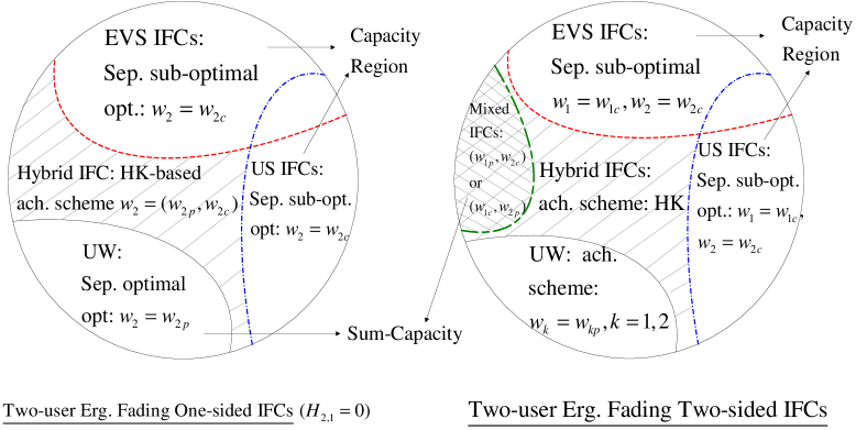
Figure 7: Overview of capacity results for two-sided and one-sided ergodic fading IFCs.

We now present examples of continuous and discrete fading process for which the channel states satisfy the EVS condition. Without loss of generality in both examples we assume that the direct links are non-fading. Thus, for the case where the fading statistics and average power constraints $\overline{P}_{k}$ satisfy the EVS conditions in (12), it is optimal for transmitter $k$ to transmit at $\overline{P}_{k}$. For the continuous model, we assume that the cross-links are independent and identically distributed Rayleigh faded links, i.e., $H_{j,k}\sim\mathcal{CN}\left(0,\sigma^{2}/2\right)$ for all $j\not=k,j,k=1,2$. For the discrete model, we assume that the cross-link fading states take values in a binary set $\left\{h_{1},h_{2}\right\}$. Finally, we set $\overline{P}_{1}=\overline{P}_{2}=\overline{P}$.

For every choice of the Rayleigh fading variance $\sigma^{2}$, we determine the maximum $\overline{P}$ for which the EVS conditions in (12) hold. The resulting feasible $\overline{P}$ vs. $\sigma^{2}$ region is plotted in Fig. 8(a). Our numerical results indicate that for very small values of $\sigma^{2}$, i.e., $\sigma^{2}<1.5$, where the cumulative distribution of fading states with $\left|H_{j,k}\right|\,<1$ is close to $1$, the EVS condition cannot be satisfied by any finite value of $\overline{P}$, however small. As $\sigma^{2}$ increases thereby increasing the likelihood of $\left|H_{j,k}\right|\,>1$, $\overline{P}$ increases too. Also plotted in Fig. 8(b) is the EVS sum-capacity achieved at $\overline{P}_{\max}$, the maximum $\overline{P}$ for every choice of $\sigma^{2}$. Furthermore, since the Rayleigh fading channel allows ergodic interference alignment [24], we compare the EVS sum-capacity with the sum-rate achieved by ergodic interference alignment for every choice of $\sigma^{2}$ and the corresponding $\overline{P}_{\max}$. This achievable scheme, whose sum-rate is the same as that achieved when the users are time-duplexed, is closer to the sum-capacity only for small values of $\sigma^{2}$. This is to be expected as EVS IFCs achieve the largest possible degrees of freedom, which is $2$ for a two-user IFC while the scheme of achieves at most one degree of freedom.

From (12), one can verify that for a non-fading very strong IFC, the very strong condition sets an upper bound on the average transmit power $\overline{P}_{k}$ at user $k$ as

$$\begin{array}[c]{cc}\overline{P}_{k}<H_{k,j}/\left(\left|H_{1,1}\right|^{2}\left|H_{2,2}\right|^{2}\right)-1&j\not=k,j,k\in\left\{1,2\right\}.\end{array}$$ (88)

One can view the upper bound on $\overline{P}$ for the EVS IFCs in Fig. 8 as an equivalent fading-averaged bound.

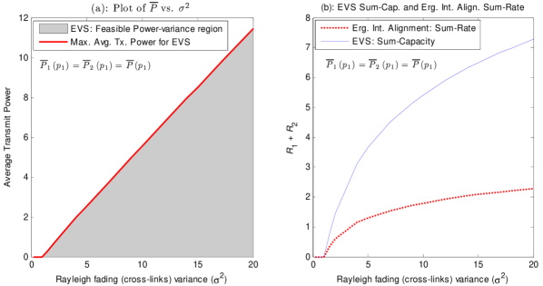
Figure 8: Feasible Power-variance region for EVS, EVS sum-capacity, and Ergodic Interference Alignment Sum-Rate.

We next compare the effect of joint and separate coding for one-sided EVS and US IFCs. For computational simplicity, we consider a discrete fading model where the non-zero cross-link fading state take values in a binary set $\left\{h_{1},h_{2}\right\}$ while the direct links are non-fading unit gains. For a one-sided EVS IFC, we choose $\left(h_{1},h_{2}\right)=\left(0.5,3.5\right)$ and $\overline{P}_{1}=\overline{P}_{2}=\overline{P}_{\max}$ where $\overline{P}_{\max}$ is the maximum power for which the EVS conditions in (12) are satisfied (note that only one of the conditions are relevant since it is a one-sided IFC). In Fig. 9, the EVS sum-capacity is plotted along with the sum-rate achieved by independent coding in each sub-channel as a function of the probability $p_{1}$ of the fading state $h_{1}$. Here independent coding means that each sub-channel is viewed as a non-fading one-sided IFC and the sum-capacity achieving strategy for each sub-channel is applied.

As expected, as $p_{1}\rightarrow 0$ or $p_{1}\rightarrow 1$, the sum-rate achieved by separable coding approaches the joint coding scheme. Thus, the difference between the optimal joint coding and the sub-optimal independent coding schemes is the largest when both fading states are equally likely. In contrast to this example where the gains from joint coding are not negligible, we also plot in Fig. 9 the sum-capacity and sum-rate achieved by independent coding for an EVS IFC with $\left(h_{1},h_{2}\right)=\left(0.5,2.0\right)$ for which the rate difference is very small. Thus, as expected, joint coding is advantageous when the variance of the cross-link fading is large and the transmit powers are small enough to result in an EVS IFC. In the same plot, we also compare the sum-capacity with the sum-rate achieved by a separable scheme for two US IFCs, one given by $\left(h_{1},h_{2}\right)=\left(1.25,1.75\right)$ and the other by $\left(h_{1},h_{2}\right)=\left(1.25,3.75\right)$. As with the EVS examples, here too, the rate difference between the optimal joint strategy and the, in general, sub-optimal independent strategy increases with increasing variance of the fading distribution.

One can similarly compare the performance of independent and joint coding for two-sided EVS and US IFCs. In this case, the more general HK scheme needs to be considered in each sub-channel for the independent coding case. In general, the observations for the one-sided also extend to the two-sided IFC.

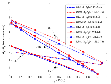
Figure 9: Plot comparing the sum-capacities and the sum-rates achieved by separable coding for different values of $\left(h_{1},h_{2}\right)$ that result in either an EVS or a US IFC.

Finally, we demonstrate sum-rates achievable by Theorem 7 for a hybrid one-sided IFC. As before, for computational simplicity, we consider a discrete fading model where the cross-link fading states take values in a binary set $\left\{h_{1},h_{2}\right\}$ while the direct links are non-fading unit gains. Without loss of generality, we choose $\left(h_{1},h_{2}\right)=\left(0.5,2.0\right)$ and assume $\overline{P}_{1}=\overline{P}_{2}=\overline{P}$. The sum-rate achieved by the proposed HK-like scheme, denoted $R_{sum}^{\left(HK\right)}$, is determined as a function of the probability $p_{1}$ of the weak state $h_{1}$. For each $p_{1}$, using the fact that a hybrid IFC is by definition one for which the EVS condition is not satisfied, we choose $\overline{P}\left(p_{1}\right)=\overline{P}_{\max}^{EVS}\left(p_{1}\right)+1.5$ where $\overline{P}_{\max}^{EVS}\left(p_{1}\right)$ is the maximum $\overline{P}$ for which the EVS conditions hold for the chosen $p_{1}$ and $\left(h_{1},h_{2}\right)$.

In Fig. 10(a), we plot $R_{sum}^{\left(HK\right)}$ as a function of $p_{1}$. We also plot the largest sum-rate outer bounds $R_{sum}^{\left(OB\right)}$ obtained by assuming interference-free links from the users to the receivers. Finally, for comparison, we plot the sum-rate $R_{sum}^{\left(Ind\right)}$ achieved by a separable coding scheme in each sub-channel. This separable coding scheme is simply a special case of the HK-based joint coding scheme presented for hybrid one-sided IFCs in Theorem 7 obtained by choosing $\alpha_{H}^{\ast}=0$ and $\alpha_{H}^{\ast}=1$ in the strong and weak sub-channels, respectively. Thus, $R_{sum}^{\left(Ind\right)}\leq R_{sum}^{\left(HK\right)}$ as demonstrated in the plot. In Fig. 10(b), the fractions $\alpha_{h_{1}}^{\ast}$ and $\alpha_{h_{2}}^{\ast}$ in the $h_{1}$ (weak) and the $h_{2}$ (strong) states, respectively, are plotted. As expected, $\alpha_{h_{2}}^{\ast}=0$; on the other hand, $\alpha_{h_{1}}^{\ast}$ varies between $0$ and $1$ such that for $p_{1}\rightarrow 1$, $\alpha_{h_{1}}^{\ast}\rightarrow 1$ and for $p_{1}\rightarrow 1$, $\alpha_{h_{1}}^{\ast}\rightarrow 1.$ Thus, when either the weak or the strong state is dominant, the performance of the HK-based coding scheme approaches that of the separable scheme in [30].

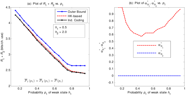
Figure 10: Sum-Rate vs. $p_{1}$ for HK-based scheme and Separable coding scheme and plots of optimal power fractions for HK-based scheme.

VII Conclusions

We have developed the sum-capacity of specific sub-classes of ergodic fading IFCs. These sub-classes include the ergodic very strong (mixture of weak and strong sub-channels satisfying the EVS condition), the uniformly strong (collection of strong sub-channels), the uniformly weak one-sided (collection of weak one-sided sub-channels) IFCs, and the uniformly mixed (mix of UW and US one-sided IFCs) two-sided IFCs. Specifically, we have shown that requiring both receivers to decode both messages, i.e., simplifying the IFC to a compound MAC, achieves the sum-capacity and the capacity region of the EVS and US (one- and two-sided) IFCs. For both sub-classes, achieving the sum-capacity requires encoding and decoding jointly across all sub-channels.

In contrast, for the UW one-sided IFCs, we have used genie-aided methods to show that the sum-capacity is achieved by ignoring interference at the interfered receiver and with independent coding across sub-channels. This approach also allowed us to develop outer bounds on the two-sided UW IFCs. We combined the UW and US one-sided IFCs results to develop the sum-capacity for the uniformly mixed two-sided IFCs and showed that joint coding is optimal.

For the final sub-class of hybrid one-sided IFCs with a mix of weak and strong sub-channels that do not satisfy the EVS conditions, using the fact that the strong sub-channels can be exploited, we have proposed a Han-Kobayashi based achievable scheme that allows partial interference cancellation using a joint coding scheme. Assuming no time-sharing, we have shown that the sum-rate is maximized by transmitting only a common message on the strong sub-channels and transmitting a private message in addition to this common message in the weak sub-channels. Proving the optimality of this scheme for the hybrid sub-class remains open. However, we have also shown that the proposed joint coding scheme applies to all sub-classes of one-sided IFCs, and therefore, encompasses the sum-capacity achieving schemes for the EVS, US, and UW sub-classes.

Analogously with the non-fading IFCs, the ergodic capacity of a two-sided IFC continues to remain unknown in general. However, additional complexity arises from the fact that the sub-channels can in general be a mix of weak and strong IFCs. A direct result of this complexity is that, in contrast to the non-fading case, the sum-capacity of a one-sided fading IFC remains open for the hybrid sub-class. The problem similarly remains open for the two-sided fading IFC. An additional challenge for the two-sided IFC is that of developing tighter bounds for the uniformly weak channel.

References

- [1] H. Sato, “The capacity of Gaussian interference channel under strong interference,” IEEE Trans. Inform. Theory, vol. 27, no. 6, pp. 786–788, Nov. 1981.
- [2] A. B. Carleial, “A case where interference does not reduce capacity,” IEEE Trans. Inform. Theory, vol. 21, no. 5, pp. 569–570, Sept. 1975.
- [3] T. S. Han and K. Kobayashi, “A new achievable rate region for the interference channel,” IEEE Trans. Inform. Theory, vol. 27, no. 1, pp. 49–60, Jan. 1981.
- [4] M. Costa, “On the Gaussian interference channel,” IEEE Trans. Inform. Theory, vol. 31, no. 5, pp. 607–615, Sept. 1985.
- [5] X. Shang, G. Kramer, and B. Chen, “A new outer bound and the noisy interference sum-rate capacity for Gaussian interference channels,” IEEE Trans. on Inform. Theory, vol. 55, no. 2, pp. 689–699, Feb. 2009.
- [6] A. Motahari and A. Khandani, “Capacity bounds for the Gaussian interference channel,” IEEE Trans. on Inform. Theory, vol. 55, no. 2, pp. 620–643, Feb. 2009.
- [7] S. Annapureddy and V. Veeravalli, “Gaussian interference networks: Sum capacity in the low interference regime and new outer bounds on the capacity region,” Feb. 2008, submitted to the IEEE Trans. Inform. Theory.
- [8] G. Kramer, “Outer bounds on the capacity of Gaussian interference channels,” IEEE Trans. on Inform. Theory, vol. 50, no. 3, pp. 581–586, Mar. 2004.
- [9] R. Etkin, D. N. C. Tse, and H. Wang, “Gaussian interference channel capacity to within one bit,” IEEE Trans. on Inform. Theory, vol. 54, no. 12, pp. 5534–5562, Dec. 2008.
- [10] I. Sason, “On achievable rate regions for the Gaussian interference channel,” IEEE Trans. on Inform. Theory, vol. 50, no. 6, pp. 1345–1356, June 2004.
- [11] Y. Weng and D. Tuninetti, “On Gaussian interference channels with mixed interference,” in Proc. 2008 IEEE Intl. Symp. Inform. Theory, Toronto, ON, Canada, July 2008.
- [12] G. Bresler and D. N. C. Tse, “The two-user Gaussian interference channel: a deterministic view,” Euro. Trans. Telecomm., vol. 19, no. 4, pp. 333–354, June 2008.
- [13] X. Shang, B. Chen, G. Kramer, and H. V. Poor, “On the capacity of MIMO interference channels,” in Proc. 46th Annual Allerton Conf. on Commun., Control, and Computing, Monticello, IL, Sept. 2008.
- [14] S. T. Chung and J. M. Cioffi, “The capacity region of frequency-selective Gaussian interference channels under strong interference,” IEEE Trans. Comm., vol. 55, no. 9, pp. 1812–1820, Sept. 2007.
- [15] C. W. Sung, K. W. K. Lui, K. W. Shum, and H. C. So, “Sum capacity of one-sided parallel Gaussian interference channels,” IEEE Trans. on Inform. Theory, vol. 54, no. 1, pp. 468–472, Jan. 2008.
- [16] X. Shang, B. Chen, G. Kramer, and H. V. Poor, “Noisy-interference sum-rate capacity of parallel Gaussian interference channels,” Feb. 2009, arxiv.org e-print 0903.0595.
- [17] S. W. Choi and S. Chung, “On the separability of parallel Gaussian interference channels,” in Proc. IEEE Int. Symp. Inform. Theory, Seoul, South Korea, June 2009.
- [18] V. R. Cadambe and S. A. Jafar, “Interference alignment and spatial degrees of freedom for the user interference channel,” IEEE Trans. on Inform. Theory, vol. 54, no. 8, pp. 3425–3441, Aug. 2008.
- [19] A. Goldsmith and P. Varaiya, “Capacity of fading channels with channel side information,” IEEE Trans. Inform. Theory, vol. 43, no. 6, pp. 1986–1992, Nov. 1997.
- [20] D. N. C. Tse and S. V. Hanly, “Multiaccess fading channels - part I: polymatroid structure, optimal resource allocation and throughput capacities,” IEEE Trans. Inform. Theory, vol. 44, no. 7, pp. 2796–2815, Nov. 1998.
- [21] D. N. C. Tse, “Optimal power allocation over parallel Gaussian broadcast channels,” http://www.eecs.berkeley.edu/ dtse/broadcast2.pdf.
- [22] L. Sankar, E. Erkip, and H. V. Poor, “Sum-capacity of ergodic fading interference and compound multiaccess channels,” in Proc. 2008 IEEE Intl. Symp. Inform. Theory, Toronto, ON, Canada, July 2008.
- [23] N. Jindal and A. Goldsmith, “Optimal power allocation for parallel broadcast channels with independent and common information,” in Proc. 2004 IEEE Int. Symp. Inform. Theory, Chicago, IL, June 2004.
- [24] B. Nazer, M. Gastpar, S. Jafar, and S. Vishwanath, “Ergodic interference alignment,” in Proc. 2009 IEEE Int. Symp. Inform. Theory, Seoul, South Korea, June 2009.
- [25] S. Jafar, “The ergodic capacity of interference networks,” Feb. 2009, arxiv.org e-print 0902.0838.
- [26] D. Tuninetti, “Gaussian fading interference channels: power control,” in Proc. 42nd Annual Asilomar Conf. Signals, Systems, and Computers, Pacific Grove, CA, Nov. 2008.
- [27] V. R. Cadambe and S. A. Jafar, “Multiple access outerbounds and the inseparability of parallel interference channels,” Feb. 2008, arxiv eprint at http://arxiv.org/cs/0802.2125.
- [28] L. Sankar, X. Shang, E. Erkip, and H. V. Poor, “Ergodic two-user interference channels,” in Proc. 2008 IEEE Intl. Symp. Inform. Theory, Toronto, ON, Canada, July 2008.
- [29] T. M. Cover and J. A. Thomas, Elements of Information Theory. New York: Wiley, 1991.
- [30] C. Sung, K. Lui, K. Shum, and H. So, “Sum capacity of one-sided parallel Gaussian interference channels,” IEEE Trans. Inform. Theory, vol. 54, no. 1, pp. 468–472, Jan. 2008.
- [31] R. Ahlswede, “The capacity region of a channel with two senders and two receivers,” Ann. Prob., vol. 2, pp. 805–814, Oct. 1974.
- [32] L. Sankar, Y. Liang, H. V. Poor, and N. B. Mandayam, “Opportunistic communications in orthogonal multiaccess relay channels,” in Proc. Int. Symp. Inf. Theory, Nice, France, July 2007.
- [33] L. Sankar, Y. Liang, N. B. Mandayam, and H. V. Poor, “Opportunistic communications in fading multi-access relay channels,” Feb. 2009, arxiv.org e-print 0902.1220.
- [34] R. Knopp and P. Humblet, “Information capacity and power control in single-cell multiuser communications,” in Proc. IEEE Intl. Conf. Commun., Seattle, WA, June 1995.
- [35] W. Yu and W. Rhee, “Iterative water-filling for Gaussian vector multiple-access channels,” IEEE Trans. Inform. Th., vol. 50, no. 1, pp. 145–152, Jan. 2004.
- [36] V. Poor, An Introduction to Signal Detection and Estimation, 2nd. Ed. Springer, 1994.