Resonant Photonic Quasicrystalline and Aperiodic Structures

Abstract

We have theoretically studied propagation of exciton-polaritons in deterministic aperiodic multiple-quantum-well structures, particularly, in the Fibonacci and Thue-Morse chains. The attention is concentrated on the structures tuned to the resonant Bragg condition with two-dimensional quantum-well exciton. The superradiant or photonic-quasicrystal regimes are realized in these structures depending on the number of the wells. The developed theory based on the two-wave approximation allows one to describe analytically the exact transfer-matrix computations for transmittance and reflectance spectra in the whole frequency range except for a narrow region near the exciton resonance. In this region the optical spectra and the exciton-polariton dispersion demonstrate scaling invariance and self-similarity which can be interpreted in terms of the “band-edge” cycle of the trace map, in the case of Fibonacci structures, and in terms of zero reflection frequencies, in the case of Thue-Morse structures.

I Introduction

Quasicrystalline and other deterministic aperiodic structures are one of the modern fields in photonics research.Merlin et al. (1985); Kohmoto and Banavar (1986); Ledermann et al. (2006); Matsui et al. (2007) Due to a long-range order such structures can form wide band gaps in energy spectra as in periodic photonic crystalsYablonovitch (1987); John (1987) and simultaneously possess localized states as in disordered media.Negro et al. (2004) The simplest and most well-studied systems consisting of only two structural building blocks are Fibonacci and Thue-Morse chains, the former one being a quasicrystal. Photonic crystals are known to allow a strong enhancement of the light-matter interaction, particularly, if the material system has elementary excitations and the light frequency is tuned to the resonant frequency of these excitations (the so-called resonant photonic crystals). In such systems the normal light waves are polaritons. The resonant properties of elementary excitations in quasiperiodic multilayered structures have been studied for plasmons and spin waves, see the review [Albuquerque and Cottam, 2003], as well as for embedded organic dye molecules.Passias et al. (2009) Whereas resonant periodic structures based on quantum wells (QWs) are widely investigated, both theoretically and experimentally,Ivchenko et al. (1994); Merle d’Aubigné et al. (1996); Hübner et al. (1996); Sadowski et al. (1997); Haas et al. (1998); Ivchenko and Willander (1999); Hayes et al. (1999); Prineas et al. (2000); Deych and Lisyansky (2000); Pilozzi et al. (2004); Ivchenko et al. (2004) aperiodic long-range ordered multiple QWs (MQWs) have attracted attention quite recently.Poddubny et al. (2008); Hendrickson et al. (2008); Werchner et al. (2009)

In Ref. Poddubny et al., 2008 we have formulated the resonant Bragg condition for the Fibonacci MQWs. We have shown that the MQW structure tuned to this condition exhibits a superradiant behaviour, for a small number $N$ of wells, and photonic-crystal-like behaviour, for large values of $N$. Moreover, in order to describe the light propagation in the infinite Fibonacci MQWs we have applied a two-wave approximation and derived equations for the edges of the two wide exciton-polariton band gaps (or pseudo-gaps) where the light waves are strongly evanescent. The fabrication and characterization of light-emitting one-dimensional photonic quasicrystals based on excitonic resonances have been reported in Refs. Hendrickson et al., 2008; Werchner et al., 2009. The measured linear and nonlinear reflectivity spectra as a function of detuning between the incident light and Bragg wavelength are in good agreement with the theoretical calculations based on the transfer-matrix approach, including the existence of a structured dip in the pronounced superradiant spectral maximum.

In this work we further develop the theory of aperiodic MQWs with particular references to the Fibonacci and Thue-Morse sequences. In Secs. II and III we define the systems under study, present the results of the exact transfer-matrix computation in the superradiant and photonic-crystal regimes and make their general analysis. In Sec. IV we apply the two-wave approximation to derive analytical formulas for the light reflection and transmission coefficients. Comparison with the exact computational results shows that the approximate description is valid in a surprisingly wide range of the light frequency $\omega$, the number $N$ of QWs, and the value of nonradiative decay rate of a two-dimensional exciton. In the close vicinity to the exciton resonance frequency $\omega_{0}$ the two-wave approximation is completely invalid. We show in Sec. V that in this region both the studied aperiodic structures demonstrate scaling invariance and self-similarity of optical properties. The main results of the paper are briefly summarized in Sec VI. In Appendix the consistency of the two-wave approximation is questioned in terms of the perturbation theory going beyond this approximation.

II Basic definitions

Here we present the definitions of the aperiodic MQW chains considered in this work. The structure consists of $N$ semiconductor QWs embedded in the dielectric matrix with the refractive index $n_{b}$. Each QW is characterized by the exciton resonance frequency $\omega_{0}$, exciton radiative decay rate $\Gamma_{0}$ and nonradiative damping $\Gamma$. We neglect the dielectric contrast assuming the background refractive index of a QW to coincide with $n_{b}$. The center of the $m$-th QW ($m=1\ldots N$) is located at the point $z=z_{m}$, and the points $z_{m}$ form an aperiodic lattice. Three ways to define a one-dimensional deterministic aperiodic lattice are based on the substitution rules,Lin et al. (1995a) analytical expression for the spacings between the lattice sites,Azbel (1979) and the cut-and-project method.Valsakumar and Kumar (1986); C.Janot (1994)

We focus on the binary sequences where the interwell spacing takes on two values, $a$ or $b$. Such structures can be associated with a word consisting of the letters $\mathcal{A}$ and $\mathcal{B}$, where each letter stands for the corresponding barrier. The QW arrangement is determined by the substitutions acting on the segments $\mathcal{A}$ and $\mathcal{B}$:

$$\mathcal{A}\to\sigma(\mathcal{A})=\mathcal{A}_{1}\mathcal{A}_{2}\ldots\mathcal{A}_{\alpha+\beta}\>,$$ (1)

$$\mathcal{B}\to\sigma(\mathcal{B})=\mathcal{B}_{1}\mathcal{B}_{2}\ldots\mathcal{B}_{\gamma+\delta}\>.$$

Each of the letters $\mathcal{A}_{k}$ and $\mathcal{B}_{k}$ in the right-hand side of Eq. (1) stands for $\mathcal{A}$ or $\mathcal{B}$, $\alpha$ and $\beta$ denote the number of letters $\mathcal{A}$ and $\mathcal{B}$ in $\sigma(A)$, $\gamma$ and $\delta$ are the numbers of $\mathcal{A}$ and $\mathcal{B}$ in $\sigma(\mathcal{B})$, respectively.Fu et al. (1997) The scattering properties of the QW sequence are described by the structure factor

$$f(q)=\lim_{N\to\infty}f(q,N)\>,$$ (2)

$$f(q,N)=\frac{1}{N}\sum_{m=1}^{N}{\rm e}^{2{\rm i}qz_{m}}\>.$$ (3)

Under certain conditionsLuck et al. (1993); Lin et al. (1995a) for the numbers $\alpha$, $\beta$, $\gamma$, $\delta$ the structure defined by Eq. (1) is a quasicrystal, so that, in the limit $N\to\infty$, the structure factor (3) consists of $\delta$-peaks responsible for the Bragg diffraction and characterized by two integers $h$ and $h^{\prime}$,

$$f(q)=\sum\limits_{h,h^{\prime}=-\infty}^{\infty}\delta_{2q,G_{hh^{\prime}}}f_{hh^{\prime}}\>,$$ (4)

$$G_{hh^{\prime}}=\frac{2\pi}{\bar{d}}\left(h+\frac{h^{\prime}}{t}\right)\ .$$ (5)

The parameter $t$ in Eq. (5) is related by

$$t=1+\frac{N_{\mathcal{B}}}{N_{\mathcal{A}}}$$ (6)

with the numbers $N_{\mathcal{B}},N_{\mathcal{A}}$ of the blocks $\mathcal{B}$ and $\mathcal{A}$ in the infinitely extending lattice. The value of $t$ in (6) can be also expressed as $t=1+(\lambda_{1}-\alpha)/\gamma$, where $\lambda_{1}=(l+\sqrt{l^{2}+4n})/2$, $l=\alpha+\delta$ and $n=\beta\gamma-\alpha\delta$; for the quasicrystals $n$ must be equal to $\pm 1$.Kolář (1993) The length $\bar{d}=(a-b)/t+b$ in Eq. (5) is the mean period of the aperiodic lattice. In the periodic case where $a\equiv b\equiv\bar{d}$, the diffraction vectors reduce to a single-index set $G_{h}=2\pi h/\bar{d}$ with the structure-factor coefficients $|f_{h}|=1$. For $a\neq b$ and irrational values of $t$, the diffraction vectors (5) fill the wavevector axis in a dense quasicontinuous way and the values of $|f_{hh^{\prime}}|$ lie inside the interval (0,1). Note that, within the uncertainty $\sim(N\bar{d})^{-1}$, the symbol $\delta_{2q,G_{hh^{\prime}}}$ in Eq. (4) is the Kronecker delta: $\delta_{2q,G_{hh^{\prime}}}=1$ when $2q=G_{hh^{\prime}}$ and zero when $2q$ is detuned from the Bragg condition. The structure factorKolář et al. (1993) defined without the prefactor $1/N$ in Eq. (3) is obtained by the replacement of the Kronecker symbol in Eq. (4) by the functional $(2\pi/\bar{d})\delta(2q-G_{hh^{\prime}})$.

The most famous one-dimensional quasicrystal is the Fibonacci sequence $\mathcal{A}\mathcal{B}\mathcal{A}\mathcal{A}\mathcal{B}\mathcal{A}\mathcal{B}\mathcal{A}\ldots$ determined by the substitutions C.Janot (1994)

$$\mathcal{A}\to\mathcal{A}\mathcal{B},\mathcal{B}\to\mathcal{A}\>.$$ (7)

For the canonical Fibonacci lattice the ratios $N_{\mathcal{A}}/N_{\mathcal{B}}$ and $a/b$ are both equal to the golden mean, $\tau=(\sqrt{5}+1)/2$. The noncanonical Fibonacci structures with $a/b\neq\tau$ are considered in Ref. Werchner et al., 2009 and are beyond the scope of this paper.

The substitution rule (7) can be generalized in many ways to provide other types of 1D quasicrystals. It has been proved in Refs. Lin et al., 1995a, Lin et al., 1995b that any binary 1D quasicrystal can be obtained by substitutions composed of different elementary inflations, e.g.,

$$\mathcal{A}\to\mathcal{A}^{n}\mathcal{B},\>\>\mathcal{B}\to\mathcal{A},\quad n=1,2\ldots\>.$$ (8)

For arbitrary values of $\alpha$, $\beta$, $\gamma$ and $\delta$ the structure defined by Eq. (1) does not form a quasicrystal. For example, the substitution

$$\mathcal{A}\to\mathcal{A}\mathcal{B},\mathcal{B}\to\mathcal{B}\mathcal{A}$$ (9)

defines the Thue-Morse lattice $\mathcal{A}\mathcal{B}\mathcal{B}\mathcal{A}\mathcal{B}\mathcal{A}\mathcal{A}\mathcal{B}\ldots$ with a singular continuous structure factor and the mean period $\bar{d}=(a+b)/2$.Cheng et al. (1988) For the Thue-Morse QW structure the function $f(q,N)$ in Eq. (3) tends to zero when $N\to\infty$ as a power of $N$ at any $q$ except certain singular values. The latter form a series

$$2q=G_{h}=\frac{\pi h}{\bar{d}},\quad h=0,\pm 1\ldots$$ (10)

with the structure factor given byLiviotti (1996)

$$|f_{h}^{({\rm TM})}|=\cos^{2}\left(\frac{\pi ah}{2\bar{d}}\right)=\cos^{2}\left(\frac{\pi bh}{2\bar{d}}\right)\>.$$ (11)

The resonant Bragg conditionPoddubny et al. (2008) for both the Fibonacci and Thue-Morse structures is formulated as

$$\frac{\omega_{0}n_{b}}{c}=\frac{G}{2}\>,$$ (12)

where $G$ stands for $G_{hh^{\prime}}$ in the Fibonacci case and for $G_{h}$ in the Thue-Morse case, see Eqs. (5) and (10), respectively. Of course, one can impose a similar condition for non-singular wavevectors contributing to the structure factor of the Thue-Morse sequence. Since in this case the value $f(q,N)$ decreases with increasing $N$ the corresponding system is far from being an efficient exciton-polaritonic structure. This is the reason why we do not consider here, e.g., the period-doubling sequence $\mathcal{A}\mathcal{B}\mathcal{A}\mathcal{A}\mathcal{A}\mathcal{B}\mathcal{A}\mathcal{B}\ldots$Liviotti (1996) determined by the rule $\mathcal{A}\to\mathcal{A}\mathcal{B},\mathcal{B}\to\mathcal{A}\mathcal{A}$, which has no Bragg peaks except for the trivial one at $q=0$.

For the sake of completeness, we also analyze a slightly disordered structure with the long-range order maintained and the QW positions defined by

$$z_{m}=m\bar{d}+\delta z_{m}\>,$$ (13)

where the deviation $\delta z_{m}$ is randomly distributed and defined by the vanishing average, $\langle\delta z_{m}\rangle=0$, and the dispersion $\sigma_{z}^{2}=\langle\delta z_{m}^{2}\rangle$. The structure factor $f(q)=\lim_{N\to\infty}f(q,N)$ of such a lattice averaged over the disorder realizations has the form

$$\langle f(q)\rangle=\sum\limits_{h}\delta_{2q,G_{h}}{\rm e}^{-(q\sigma_{z})^{2}/2},\quad G_{h}=2\pi h/\bar{d}\>.$$ (14)

The dispersion of $f(q,N)$ tends to zero with $N\to\infty$, and Eq. (14) provides a good estimation of the structure factor for any fixed disorder realization whenever $N\gtrsim 10$. The long-ranged correlations of QW positions are preserved by (13), and the Bragg diffraction is possible with the same diffraction vectors as in the periodic lattice. However, the structure-factor coefficients drop drastically with the growth of $\sigma_{z}$. The exponential factor in (14) is equivalent to the Debye-Waller factor caused by the thermal motion of atoms in a crystalline lattice.C.Kittel (1996)

Since the geometry of MQW structures under study is now described and the resonant Bragg condition is imposed we proceed to the optical reflection spectra.

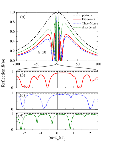
Figure 1: (Color online) Reflection spectra calculated for four QW structures, each containing $N=50$ wells and tuned to the resonant Bragg condition $2\bar{d}=\lambda(\omega_{0})$: periodic structure, with $a\equiv b\equiv\bar{d}$ (dashed); Fibonacci chain, with $a/b=\tau$ (solid curve); Thue-Morse sequence with $a/b=3/2$ (dotted); and weakly disordered periodic with $\sigma_{z}=\lambda_{0}/20$ (dashed-and-dotted). Note the break on abscissa axis on the panel (a) around $\omega=\omega_{0}$. Panels (b), (c) and (d) show the same spectra in larger scale of the variable $(\omega-\omega_{0})/\Gamma_{0}$. Calculated for $\hbar\Gamma_{0}=50~{}\mu$eV, $\hbar\omega_{0}=1.533$ eV, $\Gamma=0.1\Gamma_{0}$.

III Two regimes in optical reflection from resonant Bragg structures

Two different regimes have been revealed in optical reflection from the periodic resonant Bragg QW structures.Ivchenko and Willander (1999); Ikawa and Cho (2002) For small enough numbers of QWs, $N\ll\sqrt{\omega_{0}/\Gamma_{0}}$ (superradiant regime), the optical reflectivity is described by a Lorentzian with the maximum value $[N\Gamma_{0}/(N\Gamma_{0}+\Gamma)]^{2}$ and the halfwidth $N\Gamma_{0}+\Gamma$. For a large number of wells, $N>\sqrt{\omega_{0}/\Gamma_{0}}$ (photonic crystal regime), the reflection coefficient is close to unity within the exciton-polariton forbidden gap and exhibits an oscillatory behaviour outside the gap. The calculations presented below demonstrate the existence of similar two regimes for the deterministic aperiodic structures.

III.1 Superradiant regime

The numerical calculation of reflection spectra is carried out using the standard transfer matrix techniqueIvchenko (2005) given with more details in Sec. V. Figure 1 presents the reflectivity $R_{N}(\omega)$ calculated for the light normally incident from the left half-space $z<0$ upon four different 50-well structures. All the four, namely, the Fibonacci, Thue-Morse, periodic and distorted periodic structures, are tuned to satisfy the Bragg resonant condition (12) which can be rewritten as $\lambda(\omega_{0})=2\bar{d}$, where $\lambda(\omega)=2\pi c/(\omega n_{b})$. This means that, for the Fibonacci structure, the value $G$ in Eq. (12) is set to $G_{hh^{\prime}}$ with $h=1,h^{\prime}=0$ and, therefore, for the four structures $G=2\pi/\bar{d}$ and their optical properties can be conveniently compared.

One can see from Fig. 1 that the condition (12) leads to high reflectivity of not only the periodic and quasicrystalline Fibonacci chainsPoddubny et al. (2008) but also the Thue-Morse and slightly-disordered periodic structures. In the region $|\omega-\omega_{0}|>20\Gamma_{0}$, far enough from the exciton resonance frequency, the four spectra have similar Lorentzian wings with the halfwidth of the order of $N\Gamma_{0}$ indicating the existence of a superradiant exciton-polariton mode. The magnitude of the wings is governed by a modulus of the structure-factor coefficient, $|f_{G}|$. For the chosen structures this value runs from $|f_{G}|=1$ (periodic structure) and $|f_{G}|=0.95$ (distorted periodic) to $|f_{G}|=0.70$ (Fibonacci) and $|f_{G}|=0.65$ (Thue-Morse). The spectral wings in Fig. 1 decline monotonously with decreasing $|f_{G}|$. In addition it should be mentioned that, for the Fibonacci QW structure tuned to $G_{hh^{\prime}}$ with $h=1,h^{\prime}=1$ and analyzed in Ref. Poddubny et al., 2008, the structure-factor coefficient is $|f_{G}|\approx 0.9$ and the spectral wings in reflectivity are raised as compared with those for the Fibonacci structure tuned to $G_{1,0}$.

In the frequency region around $\omega_{0}$ the reflection spectra from the non-periodic structures show wide dips where the reflection coefficient oscillates with the period of oscillations decreasing as $\omega$ approaches $\omega_{0}$. As shown below, see also Ref. Poddubny et al. (2008), the spectral dip naturally appears for a multi-layered deterministic system tuned to a Bragg diffraction vector with the structure-factor coefficient $f_{G}$ smaller than unity, and it widens as the value of $1-|f_{G}|$ increases.

For small values of the exciton nonradiative damping rate $\Gamma$ (lying beyond experimentally available values), the fine structure of optical spectra in the narrow resonance region ranged over few $\Gamma_{0}$ is very intricate, see Figs. 1(b)–1(d). All the considered aperiodic structures possess a narrow middle stop-band embracing the exciton resonance $\omega_{0}$. In particular, for the Fibonacci QW structure this stop-band is located between $\omega_{0}-0.4\Gamma_{0}$ and $\omega_{0}+0.9\Gamma_{0}$. The spectral properties in the frequency range $|\omega-\omega_{0}|\sim\Gamma_{0}$ for $\Gamma\ll\Gamma_{0}$ are discussed in Sec. V in more details.

In realistic semiconductor QWs the nonradiative decay rate is larger than (or comparable with) $\Gamma_{0}$, and the majority of spectral fine-structure features are smoothed.Hendrickson et al. (2008) The influence of the nonradiative damping on the reflectivity from the Fibonacci MQWs is illustrated in Fig. 2. Thin curve on the upper panel is the same as that on Fig. 1 and calculated for $\Gamma=0.1\Gamma_{0}$ while the thick curve corresponds to more realistic value $\Gamma=2\Gamma_{0}$. One can trace the smoothing of sharp spectral features with increasing $\Gamma$. However, some of these features may still be resolved by means of the differential spectroscopy widely used in studies of bulk crystals and low-dimensional structures.Makhniy et al. (2006) Panels (b) and (c) of Fig. 3 present the first and second derivatives $R^{\prime}(\omega)\equiv\partial R(\omega)/\partial\omega$ and $R^{\prime\prime}(\omega)$, respectively. The differential spectra allow one to enhance the spectral peculiarities poorly resolved in the ordinary spectrum of Fig. 2(a).

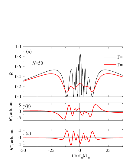
Figure 2: (Color online) Differential reflection spectra calculated for Fibonacci QW structures containing $N=50$ wells. Panel (a) shows reflection spectrum $R(\omega)$ calculated for $\Gamma=0.1\Gamma_{0}$ (thin curve) and $\Gamma=2\Gamma_{0}$ (thick curve). Panels (b) and (c) demonstrate the first- and second-order differential spectra $R^{\prime}(\omega)$ and $R^{\prime\prime}(\omega)$ in arbitrary units for $\Gamma=2\Gamma_{0}$. Other parameters are the same as in Fig. 1.

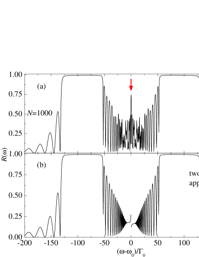
Figure 3: (Color online) Reflection spectra calculated for a Fibonacci QW structure containing 1000 wells. The parameters used are the same as those in Fig. 1 except for the nonradiative decay which now is $\Gamma=0.2\Gamma_{0}$. Upper and lower panels correspond, respectively, to the exact calculation and calculation in the two-wave approximation. Vertical arrow at $\omega=\omega_{0}$ in panel (a) indicates the narrow reflectivity stop-band, which cannot be described by the two-wave approximation.

III.2 Photonic-quasicrystal regime

The superradiant regime holds up to $N\sim 100$ and is followed by a saturation with the further increase in the number of QWs.Ikawa and Cho (2002) In this subsection we study very long QW chains with $N\gg\sqrt{\omega_{0}/\Gamma_{0}}$. The calculations for $N=1000$ are presented in Fig. 3 for Fibonacci MQWs and Fig. 4 for Thue-Morse MQWs. Figure 3 allows a clear interpretation of the spectral properties of excitonic polaritons. Two symmetric stop-bandsPoddubny et al. (2008) standing out between numerous sharp maxima and minima are clearly seen in the spectra. Figure 3(b) shows the spectrum calculated in the two-wave approximation taking into account only three terms in the sum (4), namely, the terms with $2q=\pm G_{1,0}$ and $2q=0$, see Sec. IV for details. Comparing Figs. 3(a) and 3(b) we conclude that a lot of spectral features are reproduced as the interference fringes in the approximated spectrum. However, this approximation lacks an adequate description of the reflection spectrum around the exciton resonance frequency. The middle stop-band at $\omega=\omega_{0}$ found in Fig. 1(b) reveals itself also in Fig. 3(a) where it is indicated by a vertical arrow.

Thin solid curve in Fig. 4 illustrates the exact reflectivity calculation for the Thue-Morse structure with $N=1000$. Thick solid curve is calculated in the two-wave approximation in the limit $N\to\infty$ so that all the interference fringes are smoothed due to the finite value of $\Gamma\to+0$. We have checked for the Thue-Morse sequence that, for $N=1000$, the two-wave approximation works well outside the narrow interval $|\omega-\omega_{0}|\sim\Gamma_{0}$. The fine features around $\omega_{0}$ are again beyond the scope of the two-wave approximation. The spectrum for 1000 periodic QWs, dotted curve in Fig. 4, is presented for comparison in order to emphasize similarities and differences between the optical spectra of periodic and aperiodic systems under consideration.

Figures 1-4 form a computational data base for the physical interpretation of the reflection spectral shapes. This can be done in terms of the two-wave approximation (Sec. IV) and scaling and self-similarity (Sec. V).

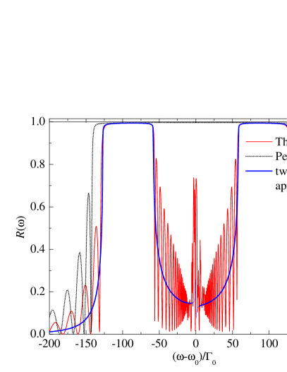
Figure 4: (Color online) Reflection spectra calculated for Thue-Morse and periodic QW structures. Thin solid curve corresponds to the exact calculation for $N=1000$ Thue-Morse QWs, thick solid curve is calculated in the two-wave approximation for $N\to\infty$. Dotted curve represents the $N=1000$ periodic MQWs with the period $d=\lambda(\omega_{0})/2$. The parameters used are the same as those in Fig. 3.

IV Optical spectra in the two-wave approximation

In this section we apply the two-wave approximation for derivation of the exciton-polariton dispersion and the reflectivity spectra of the aperiodic resonant Bragg MQW structures. The derivation is performed for the particular case of a canonic Fibonacci chain but the results can be straightforwardly generalized to noncanonical quasicrystal sequences and other deterministic aperiodic multi-layered structures.

The electric field of the light wave propagating in the MQW structure satisfies the following wave equationIvchenko (2005)

$$\left(-\frac{d^{2}}{dz^{2}}-q^{2}\right)E(z)=\frac{2q\Gamma_{0}}{\omega_{0}-\omega-{\rm i}\Gamma}\sum_{m}\delta(z-z_{m})E(z_{m})\>.$$ (15)

Assuming the resonant Fibonacci MQWs to contain a sufficiently large number $N$ of wells we replace the structure factor $f(q,N)$ by its limit $f(q)$ given by Eq. (4). This allows one to approximate solutions of Eq. (15) as a superposition of the “Bloch-like” waves

$$E_{K}(z)=\sum\limits_{h,h^{\prime}}{\rm e}^{{\rm i}(K-G_{hh^{\prime}})z}E_{K-G_{hh^{\prime}}}\>.$$ (16)

As distinct from the true Bloch functions in a periodic system, here the countable set of vectors $G_{hh^{\prime}}$ is enumerated not by one but by two integer numbers, $h$ and $h^{\prime}$, see Eq. (5). Substituting $E_{K}(z)$ into Eq. (15), multiplying each term by $\exp[-{\rm i}(K-G_{hh^{\prime}})z]$ with particular $h,h^{\prime}$ and integrating over $z$ we obtain

$$\begin{split}[q^{2}-(K-&G_{hh^{\prime}})^{2}+2q\xi]E_{K-G_{hh^{\prime}}}+\\ &2q\xi\sum\limits_{gg^{\prime}}f^{*}_{g-h,g^{\prime}-h^{\prime}}E_{K-G_{gg^{\prime}}}=0\>,\end{split}$$ (17)

where

$$\xi(\omega)=\frac{\Gamma_{0}}{{\bar{d}}(\omega_{0}-\omega-{\rm i}\Gamma)}\>.$$ (18)

Note that, throughout this paper, we focus on a frequency region $|\omega-\omega_{0}|\ll\omega_{0}$ around the exciton resonance.

In accordance with Eq. (12) we consider the Fibonacci QW structure tuned to the Bragg resonance

$$\frac{\omega_{0}}{c}n_{b}\equiv q_{0}=\frac{G_{h,h^{\prime}}}{2}\>.$$ (19)

In the two-wave approximation, only two space harmonics $K$ and $K^{\prime}=K-G_{hh^{\prime}}=K-2q_{0}$ are taken into account in the superposition (16). A necessary but not sufficient condition for validity of this approximation is the inequality

$$\left|q_{0}-K\right|\ll q_{0}\ .$$ (20)

Then the infinite set (17) is reduced to a system of two coupled equations

$$(q-K+\xi)E_{K}+\xi f^{*}_{hh^{\prime}}E_{K^{\prime}}=0\>,$$ (21)

$$\xi f_{hh^{\prime}}E_{K}+(q+K-2q_{0}+\xi)E_{K^{\prime}}=0\>.$$

The two eigenvalues $K$ corresponding to the frequency $\omega$ are given by

$$K^{(\pm)}=q_{0}\pm Q\>,\>Q=\sqrt{(\xi+q-q_{0})^{2}-\xi^{2}|f_{hh^{\prime}}|^{2}}\>.$$ (22)

The criterion (20) is then rewritten in the form

$${\rm max}\{|\omega_{0}-\omega|,\Gamma\}\gg\Gamma_{0}\frac{\sqrt{1-|f_{hh^{\prime}}|^{2}}}{h+h^{\prime}/\tau}\ .$$ (23)

At $f_{hh^{\prime}}\to 1$ this dispersion equation reduces to that for the periodic resonant Bragg MQWsIvchenko and Willander (1999)

$$Q=q_{0}\sqrt{\left(\frac{\omega-\omega_{0}}{\omega_{0}}\right)^{2}-\Delta^{2}\frac{\omega-\omega_{0}}{\omega-\omega_{0}+{\rm i}\Gamma}}\>,$$

where

$$\Delta=\sqrt{\frac{2\Gamma_{0}\omega_{0}}{\pi}}\ .$$

The edges, $\omega_{\rm out}^{\pm}$ and $\omega_{\rm in}^{\pm}$, of two symmetrical band gaps in the Fibonacci QW structure are obtained from Eq. (22) by setting $K^{(\pm)}=q_{0}$ or, equivalently, $Q=0$. The result readsPoddubny et al. (2008)

$$\omega_{\rm out}^{\pm}=\omega_{0}\pm\Delta\sqrt{\frac{1+|f_{hh^{\prime}}|}{2\>(h+h^{\prime}/\tau)}}\>,$$ (24)

$$\omega_{\rm in}^{\pm}=\omega_{0}\pm\Delta\sqrt{\frac{1-|f_{hh^{\prime}}|}{2\>(h+h^{\prime}/\tau)}}\>.$$

As shown in Appendix, for the exciton-polariton waves at the bandgap edges located at the point $K=q_{0}$, an admixture of other space harmonics has no remarkable influence and these edges are well-defined for the resonant QW Fibonacci chains. For each frequency lying inside the interval between the edges $\omega_{\rm in}^{-}$ and $\omega_{\rm in}^{+}$, the two-wave approximation gives two linearly independent solutions $K^{(\pm)}=q_{0}\pm Q$ with nonzero $Q$. An exciton-polariton wave induced by the initial incoming light wave is a superposition of these two Bloch-like solutions. They can be coupled by the diffraction wavevector $G_{gg^{\prime}}$ satisfying the condition $2Q=G_{gg^{\prime}}$. If the corresponding structure-factor coefficient $f_{gg^{\prime}}$ is remarkable one should include into consideration mixing of the waves $K^{(\pm)}$ which complicates the comparatively simple description of exciton polaritons. In the approximate approach we will ignore the diffraction-induced mixing between the waves $K^{(\pm)}$ and analyze the validity of this description by comparing the exact and two-wave calculations.

In order to derive an analytical expression for the reflection coefficient from an $N$-well chain sandwiched between the semiinfinite barriers (material B) we write the field in the three regions, the left barrier, the MQWs and the right barrier, as follows

$$E(z)=\begin{cases}e^{{\rm i}qz}+r_{N}e^{-{\rm i}qz}\quad&(z<0)\>,\\ E_{+}{\rm e}^{{\rm i}Qz}({\rm e}^{{\rm i}q_{\mbox{}_{0}}z}+\zeta_{+}{\rm e}^{-{\rm i}q_{\mbox{}_{0}}z})+\\ \quad E_{-}{\rm e}^{-{\rm i}Qz}({\rm e}^{{\rm i}q_{\mbox{}_{0}}z}+\zeta_{-}{\rm e}^{-{\rm i}q_{\mbox{}_{0}}z})\quad&(0<z<N\bar{d})\>,\\ t_{N}e^{iq(z-N\bar{d})}\quad&(N\bar{d}<z)\>.\end{cases}$$ (25)

Here $r_{N}$ and $t_{N}$ are the reflection and transmission amplitude coefficients, $E_{\pm}$ are the amplitudes of the “Bloch-like” solutions, and

$$\zeta_{\pm}=-\frac{\xi f_{hh^{\prime}}}{q-q_{0}\pm Q+\xi}\>.$$

Values of $r_{N},t_{N},E_{+},E_{-}$ are related by imposing the boundary conditions which are continuity of the electric field $E(z)$ and its first derivative $dE(z)/dz$ at the points $z_{1}=0$ and $z_{N}$. If the number of wells $N$ coincides with $N=F_{j}+1$, where $F_{j}$ is one of the Fibonacci numbers, then the product $G_{hh^{\prime}}z_{N}$ differs from an integer multiply of $2\pi$ by a negligibly small value, $\delta_{N}=-G_{hh^{\prime}}s(1-\tau)^{j-1}\tau^{-2}$. In this case the phase factor $\exp{({\rm i}G_{hh^{\prime}}z_{N})}$ can be replaced by unity and the straightforward derivation results in surprisingly simple expressions for the reflection coefficient,

$$r_{N}=\frac{\xi f_{hh^{\prime}}}{q_{0}-q-\xi-{\rm i}Q\cot{(QN\bar{d})}}\>,$$ (26)

and for the transmission coefficient, ${t_{N}=-{\rm i}r_{N}Q/[\xi f_{hh^{\prime}}\sin{(QN\bar{d})}]}$.

Numerical calculation demonstrates that in the region (23) the two-wave approximation is valid even for the Fibonacci structures with $N\neq F_{j}+1$ provided that $N\gtrsim 20$ and the mesoscopic effects are reduced. Moreover, Eq. (26) for the reflection coefficient can be applied to other deterministic aperiodic systems including the Thue-Morse and weakly disordered periodic structures. It suffices for the structure to be characterized by a single value of the structure factor at particular vector which can play the role of the Bragg diffraction vector. In the crystalline case where $f_{hh^{\prime}}\equiv 1$ analogous approximation describes the nuclear resonant scattering of $\gamma$-rays.Kagan (1999)

The two-wave approximation can be generalized to allow for the dielectric contrast, i.e., the difference between the dielectric constant of the barrier, $n_{b}^{2}$, and the background dielectric constant of the QW, $n_{a}^{2}$. In a structure with $n_{a}\neq n_{b}$ the stop-band exists even neglecting the exciton effect, $\Gamma_{0}=0$. The excitonic resonance leads to the splitting of this single stop-band to two ones. In the periodic case the highest reflectivity is reached when the two stop-bands touch each other and form a single exciton-polariton gap. This is the effective Bragg condition for the periodic structure with the dielectric contrast.Ivchenko et al. (2004) In the Fibonacci case when $|f_{hh^{\prime}}|<1$ the stop bands never touch each other and the Bragg condition means that the sum of their widths reaches a maximum. For the realistic case of a small contrast, $|n_{a}-n_{b}|\ll n_{a},n_{b}$, this condition is equivalent to the tuning of the exciton resonance frequency $\omega_{0}$ to one of the edges of the stop-band found at $\Gamma_{0}=0$, similarly to the condition for the periodic structures.Ivchenko et al. (2004); Ivchenko and Poddubny (2006). Note that the reflectivity spectrum taken from the Bragg MQW structure with the dielectric contrast is always asymmetric.

For periodic resonant Bragg MQWs, in the superradiant regime $N\ll\sqrt{\omega_{0}/\Gamma_{0}}$, Eq. (26) is readily transformed to the well-known resultIvchenko et al. (1994)

$$r_{N}(\omega)=\frac{{\rm i}N\Gamma_{0}}{\omega_{0}-\omega-{\rm i}(N\Gamma_{0}+\Gamma)}\>.$$ (27)

The pole at $\omega=\omega_{0}-{\rm i}(N\Gamma_{0}+\Gamma)$ is the eigenfrequency of the superradiant mode. In general, the eigenfrequencies $\omega^{(l)}$ of a MQW structure are represented by zeros of the denominator in Eq. (26). Since the structure is open the eigenfrequencies are complex even in the absence of nonradiative damping, $\Gamma=0$. Values of $\omega^{(l)}$ lying in the region

$$|\omega-\omega_{0}|\ll\frac{\Delta\sqrt{1-|f_{hh^{\prime}}|}}{\sqrt{h+h^{\prime}/\tau}}$$ (28)

but outside the narrow interval (23) can be easily found taking into account that, in this region, the difference $q_{0}-q$ in Eqs. (22), (26) can be neglected as compared with $\xi$ so that one has $Q=\xi\sqrt{1-|f_{hh^{\prime}}|^{2}}$ and

$$\omega^{(l)}=\omega_{0}-{\rm i}\Gamma-{\rm i}N\Gamma_{0}\frac{\sqrt{1-|f_{hh^{\prime}}|^{2}}}{\mathop{\mathrm{missing}}{arctanh}\nolimits(\sqrt{1-|f_{hh^{\prime}}|^{2}})+{\rm i}\pi l}\ ,$$

$$l=0,\pm 1,\pm 2\ldots$$ (29)

Equation (29) determines at $l=0$ the frequency of the superradiant mode. In the particular case $1-|f_{hh^{\prime}}|^{2}\ll 1$, this frequency is given by

$$\omega^{(0)}=\omega_{0}-{\rm i}N\Gamma_{0}\left(\frac{2}{3}+\frac{|f_{hh^{\prime}}|^{2}}{3}\right)\>.$$ (30)

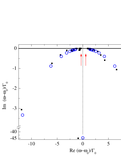
Figure 5: (Color online) Complex eigenfrequencies of exciton polaritons in Fibonacci 56-QW structure calculated exactly (filled symbols) and in the two-wave approximation (empty symbols). Note the break at the ordinate axis. Vertical arrows indicate the edges of inner stop-band. Calculated for $\Gamma=0$ and other parameters same as in Fig. 1

Figure 5 shows the eigenfrequencies of a $56$-QW Fibonacci structure calculated exactly (filled symbols) and from Eq. (29) (closed symbols). The exact calculation is performed using the system of coupled equation for excitonic polarization $P_{m}$ in the quantum wellIvchenko (2005)

$$(\omega_{0}-\omega-{\rm i}\Gamma)P_{m}+\sum\limits_{m^{\prime}=1}^{N}e^{{\rm i}q|z_{m}-z_{m}^{\prime}|}P_{m^{\prime}},\quad m=1\ldots N\>.$$ (31)

One can see from Fig. 5 that the two-wave approximation excellently describes the superradiant mode as well as some of the subradiant modes lying far from $\omega_{0}$ on the complex plane. The approximation breaks in the region close to $\omega_{0}$ where more sophisticated analysis is required, as presented in the next Section.

V Optical spectra near the exciton resonance frequency

V.1 Trace map technique for Fibonacci and Thue-Morse quantum well structures

In this section we concentrate on the narrow frequency region $|\omega-\omega_{0}|\sim\Gamma_{0}$. A convenient and powerful tool for such study is the transfer matrix method. The substitution rules (1) lead to recursive relations for the transfer matrices providing all the essential information about the spectral properties of MQWs.

In the following we use the notation $\mathcal{F}_{j}$ for the Fibonacci chain containing $N=F_{j}$ QWs starting from the trivial chain $\mathcal{F}_{1}$ that consists of one segment $\mathcal{A}$. Similarly, $\mathcal{TM}_{j}$ is the Thue-Morse sequence with $N=2^{j}$ QWs starting from $\mathcal{TM}_{0}=\mathcal{A}$. The transfer matrix $M_{j}$ through the whole structure $\mathcal{F}_{j}$ or $\mathcal{TM}_{j}$ is given by a product of the matrices $M_{\rm QW}$, $M_{\rm A}$, $M_{\rm B}$ of transfer through a QW and a barrier of length $a$ or $b$, respectively, with the order established by the chain definition (1). In the basis of electric field $E(z)$ and its derivative $-q^{-1}dE(z)/dz$ the transfer matrices are as followsIvchenko (2005)

$$M_{\rm QW}=\begin{pmatrix}1&0\\ 2S&1\end{pmatrix}\>,\>S=\frac{\Gamma_{0}}{\omega_{0}-\omega-i\Gamma}\>,$$ (32)

and Brehm (1991)

$$M_{\mathcal{D}}=\begin{pmatrix}\cos{qd}&-\sin{qd}\\ \sin{qd}&\cos{qd}\end{pmatrix},\quad\mathcal{D}={\rm A},{\rm B};d=a,b\>.$$ (33)

We will here restrict ourselves to the limit of zero nonradiative decay, $\Gamma=0$, in which case the transfer matrices are real. The transmission and reflection spectra, $T_{j}(\omega)$ and $R_{j}(\omega)$, are given byBrehm (1991)

$$T_{j}(\omega)=1-R_{j}(\omega)=\frac{1}{x_{j}^{2}(\omega)+y_{j}^{2}(\omega)}\>.$$ (34)

Here the quantities $x_{j}$ and $y_{j}$ stand for the half-trace $(M_{j,11}+M_{j,22})/2$ and half-antitrace $(M_{j,21}-M_{j,12})/2$ of the matrix $M_{j}$, respectively.

In order to reveal the behavior of exciton polaritons in aperiodic MQWs it is instructive to calculate the polariton dispersion in the approximantsAzbel (1979) of the aperiodic chains containing the periodically repeating sequences $\mathcal{F}_{j}$ or $\mathcal{TM}_{j}$. In such periodic systems the polariton band structure consists of allowed minibands and forbidden gaps. The gaps are found from the conditionIvchenko (2005)

$$|x_{j}(\omega)|>1\>.$$ (35)

To proceed to the analysis of the pattern of allowed and forbidden bands we note that the half-traces $x_{j}$ of the substitution sequences satisfy closed recurrence relations, also termed as trace maps.Kolář and Ali (1990) For the Fibonacci and Thue-Morse chains, the trace maps read

$$x_{j+1} =2x_{j}x_{j-1}-x_{j-2} \text{(Fibonacci)}\>,$$ (36a)

$$x_{j+1} =4x_{j-1}^{2}(x_{j}-1)+1 \text{(Thue-Morse)}\>.$$ (36b)

Consequently, the polariton energy spectrum is determined by the general properties of nonlinear transformations (36) and the initial conditions specific for the QW transfer matrices (32). The trace maps are effective for studies of the spectral properties of deterministic aperiodic structures.Kohmoto and Banavar (1986); Lin et al. (1995a)

V.2 Scaling of band structure and transmission spectra in Fibonacci structures

We will now analyze the band structure and the transmission spectra in Fibonacci QW structures. For the Fibonacci lattices the trace map (36a) possesses an invariantKohmoto and Oono (1984)

$$I=x_{j}^{2}+x_{j+1}^{2}+x_{j+2}^{2}-2x_{j}x_{j+1}x_{j+2}-1\>.$$

In the QW structure this invariant can be reduced to

$$I(\omega)=S^{2}(\omega)\sin^{2}[qb(\tau-1)]\>.$$ (37)

The resonant behavior of this invariant as a function of frequency indicates that the band structure for Fibonacci QW chains may be very complex in the region $|\omega-\omega_{0}|\sim\Gamma_{0}$. The band calculations are presented in Fig. 6(a), where the black stripes and horizontal lines show, respectively, the forbidden and allowed bands for different values of the structure order $j$ ranging from $j=1$ to $j=13$. Figures 6(b)-6(d) represent this band sequence for $j=11$ and $j=13$ in different frequency scales. Panel (a) demonstrates that two broad band gaps are already present for 21 QWs ($j=8$). With increasing $j$ their edges very quickly converge to the analytical values (24) shown by the gray rectangles in Fig. 6(a). A narrow permanent middle band gap at $-0.4\Gamma_{0}\lesssim\omega-\omega_{0}\lesssim 0.9\Gamma_{0}$ is well resolved in the scale of Fig. 6(b).

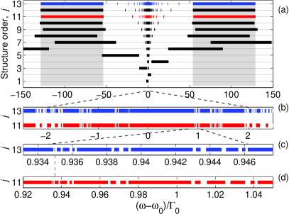
Figure 6: (Color online) (a). Exciton-polariton allowed (thin lines) and forbidden (thick stripes) bands in periodically repeated Fibonacci sequences of the order $j=1\ldots 13$. (b) Bands for $j=11$ ad $j=13$ in the spectral range around the frequency $\omega=\omega_{0}$. (c),(d) Bands for $j=11$ and $j=13$, respectively, in a large scales near the frequency $\omega=\omega_{0}+0.935\Gamma_{0}$ indicated by the vertical line. Calculated for $\Gamma=0$ and other parameters same as in Fig. 1

The other forbidden bands depicted in Fig. 6 can be interpreted in terms of two formation mechanisms. The first mechanism is related to the two-wave approximation. In this approximation the half-trace of the transfer matrix $x_{j}$ reaches minimum ($-1$) or maximum (+1) values at particular frequencies $\omega_{s}$ where the reflectivity $r_{N}^{({\rm 2w})}$ vanishes. One can check from Eq. (26) that at these frequencies the product $QN\bar{d}$ is an integer number of $\pi$. In the vicinity of $\omega_{s}$ one can approximate $x^{({\rm 2w})}(\omega)$ by $n_{s}[1-u_{s}(\omega-\omega_{s})^{2}]$, where $n_{s}=\pm 1$, and $u_{s}$ is a positive coefficient. Near $\omega_{s}$ the exact function $x_{j}(\omega)\equiv{\rm Tr}(M_{j})/2$ differs from $x^{({\rm 2w})}(\omega)$ by the correction $\delta x(\omega)$ which can be approximated by $n_{s}[c_{s}+v_{s}(\omega-\omega_{s})]$ where $c_{s},v_{s}$ are additional constants. As a result the behavior of the half-trace can be presented in the form

$$x(\omega)=n_{s}\left[1+c_{s}+\frac{v_{s}^{2}}{4u_{s}}-u_{s}\left(\omega-\omega_{s}-\frac{v_{s}}{2u_{s}}\right)^{2}\right]\>.$$

If $c_{s}+(v_{s}^{2}/4u_{s})$ is positive then the periodic system has a gap at $\omega^{\prime}_{s}=\omega_{s}+(v_{s}/2u_{s})$.

The second mechanism of gap formation is related to localized exciton-polariton states rather than to the Fabry-Perot interference and can be treated in terms of self-similarity effects. Particularly, in the frequency range $|\omega-\omega_{0}|\sim\Gamma_{0}$ the number of stop-bands increases while their widths tend to zero as $N\to\infty$. As a result, the sequence of the allowed and forbidden bands becomes quite intricate, see Figs. 6(b)–6(d), and locally resembles the Cantor set.Kohmoto and Oono (1984) The most striking result in Fig. 6(b) is similarity of the band structure of the approximants with $j=11$ and $j=13$. On the other hand, the spectrum for $j=13$ has a lot of narrow band gaps not resolved in the scale of Fig. 6(b). Figures 6(c) and 6(d) present the same spectra in larger scales near the right edge of the middle band gap, with the scale for $j=13$ being $\lambda_{+}\approx 8$ times larger than that for $j=13$. Matching the bandgap positions we prove an existence of the spectral scaling in the Fibonacci QW structures. The scaling index $\lambda_{+}$ specifies the ratio of the widths of spectral features of the structures with the order differing by two. The scaling properties hold not only for the band positions but for the whole curves $x_{j}(\omega)$, as Fig. 7 demonstrates for $j=11,13$ and 15. One can see that the curves plotted in the proper scales repeat each other almost exactly.

Now we turn from the transfer matrix traces analysis, to the complex eigenfrequencies (31) and to the transmission spectra $T_{j}(\omega)$. The spectra $T_{j}(\omega)$ for the resonant Fibonacci structures are shown in Fig. 8 for $j=11$ ($N=89$ QWs) and $j=13$ ($N=234$ QWs) in the frequency region adjacent to the right edge of the middle band gap. The real parts of the complex eigenfrequencies are indicated by the vertical lines. The abscissa scales on Figs. 8(a) and 8(c) are the same as in Figs. 6(d) and 6(c). Examining Fig. 8 we conclude, that the scaling properties revealed by Figs. 6 and 7, are also manifested in the optical spectra. Indeed, comparing Fig. 8(a) and Fig. 8(b) we find that the general shape of the spectra remains similar although more details appear when $N$ grows. On the other hand, the relative distances between the transmission peaks for $j=13$ in the large scale agree with those for $j=11$ in a smaller scale, cf. Fig. 8(a) and Fig. 8(c). The positions of the real parts of complex eigenfrequencies correspond to the peaks in the transmission spectra and exhibit the same scaling behaviour. Such behavior is also demonstrated at the left edge of the middle bandgap $\omega-\omega_{0}\sim-0.37\Gamma_{0}$, it is characterized by the scaling index $\lambda_{-}\sim 16$.

The self-similarity of band structure of Fibonacci sequences with the orders $j$ differing by 2 can be related to the so-called “band-edge” cycle of the trace map (36a).Kohmoto et al. (1987) This can be done by the following consideration. If the half-traces $x_{j}$ for three successive orders $j=j_{0},j_{0}+1,j_{0}+2$ are interrelated by

$$x_{j_{0}+1}=-\frac{x_{j_{0}}}{2x_{j_{0}}-1}\>,\>x_{j_{0}+2}=-x_{j_{0}}$$ (38)

then according to the recurrent equations (36a) the values of $x_{j}$ for $j\geq j_{0}$ form a periodic sequence

$$x^{*},-\frac{x^{*}}{2x^{*}-1},-x^{*},\frac{x^{*}}{2x^{*}-1},-x^{*},-\frac{x^{*}}{2x^{*}-1},x^{*},\ldots$$ (39)

where $x^{*}=x_{j_{0}}$. Although the sequence (39) repeats itself only after 6 iterations, the length of the cycle for the absolute value of the trace is two.

Considering $x_{j}$ as functions of the frequency $\omega$ we introduce solutions $\omega^{(a)}(j_{0})$ and $\omega^{(b)}(j_{0})$ of the first and second equations (38). The numerical calculation shows that, for each $j_{0}$, in the vicinity of $\omega_{0}$ there exist two pairs of solutions, $\omega^{(a)}_{\pm}(j_{0})$, and $\omega_{\pm}^{(b)}(j_{0})$. Moreover, values of $\omega^{(a)}_{+}(j_{0})$ and $\omega_{+}^{(b)}(j_{0})$ or $\omega^{(a)}_{-}(j_{0})$ and $\omega_{-}^{(b)}(j_{0})$ merge with increasing $j_{0}$, and one can introduce the asymptotic frequencies $\omega^{*}_{\pm}=\omega^{(a)}_{\pm}(j_{0}\to\infty)=\omega^{(b)}_{\pm}(j_{0}\to\infty)$, with the values $\omega^{*}_{+}\approx 0.94\Gamma_{0}$ and $\omega^{*}_{-}\approx-0.37\Gamma_{0}$ .

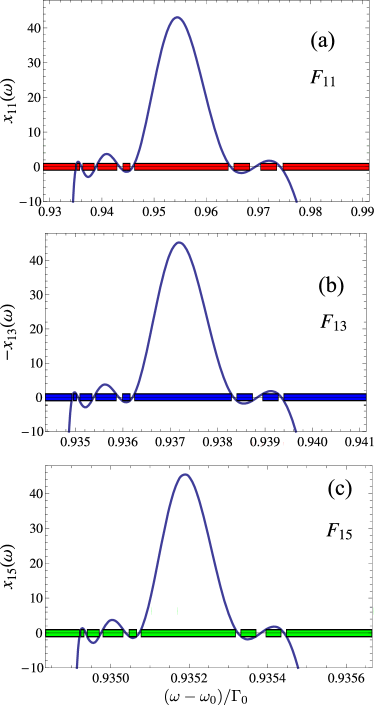
Figure 7: (Color online) Trace scaling for the Fibonacci structures. The panels (a), (b) and (c) show the half-trace $x_{j}(\omega)$ for $j=11,13,15$, respectively. The filled ribbons indicate the regions of polariton band gaps, where $|x_{j}(\omega)|>1$. Calculated for $\Gamma=0$ and other parameters same as in Fig. 1

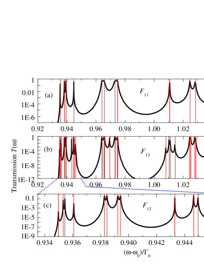
Figure 8: (Color online) Transmission spectra of the Fibonacci quantum-well sequences of the order $j=$11(a), and $j=$13 (b,c), containing $89$ and $233$ QWs, respectively. Vertical lines indicate the real parts of complex eigenfrequencies of the structures. Calculated for $\Gamma=0$ and other parameters same as in Fig. 1

Our analysis made for Fibonacci structures with different pair values of $(h,h^{\prime})$ shows that they also demonstrate analogous scaling behaviour in the vicinity of $\omega_{0}$. The distance $|\omega_{+}^{*}-\omega_{-}^{*}|$ between the scaling frequencies decreases with the growth of the barrier thicknesses. The scaling indices increase, when the middle band gap becomes narrower. We have established that there exists the following equation relating the scaling indices and the frequencies $\omega^{*}_{\pm}$:

$$\lambda_{\pm}\approx\Lambda_{1}+\Lambda_{2}\sqrt{I(\omega_{\pm}^{*})}\equiv\Lambda_{1}+\frac{\Lambda_{2}\Gamma_{0}}{|\omega_{0}-\omega_{\pm}^{*}|}\bigl{|}\sin\bigl{[}q(\omega_{0})b(\tau-1)\bigr{]}\bigr{|}\>.$$ (40)

The coefficients $\Lambda_{1}$ and $\Lambda_{2}$ are found to be close to 3 and 4, respectively, and are independent of the structure parameters. Since the value of $|\omega^{*}_{+}-\omega_{0}|/\Gamma_{0}\approx 0.94$ exceeds $|\omega^{*}_{-}-\omega_{0}|/\Gamma_{0}\approx 0.37$ the scaling coefficient $\lambda_{+}\approx 8$ is smaller than $\lambda_{-}\approx 16$.

We have also analyzed the spatial structure of the excitonic polarization $P_{m}$ of the eigenstates satisfying Eq. (31). In particular, this distribution is characterized by the participation ratio $p=\sum_{m=1}^{N}|P_{m}|^{4}/\bigl{(}\sum_{m=1}^{N}|P_{m}|^{2}\bigr{)}^{2}$, where the sum runs over QW-lattice sites.Zekri and Brezini (1992) The parameter $p$ is a measure of the state localization-delocalization: for a completely delocalized state $p\approx 1/N$, whereas $p\approx 1$ for a state tied to a single site. In the periodic Bragg structure with $\bar{d}=\lambda(\omega_{0})/2$, the superradiant mode is described by the eigenvector $P_{m}=(-1)^{m}P_{0}$ and the participation ratio $p=1/N$. In the Fibonacci QW chain the participation ratio remains small for the superradiant mode as well as for the subradiant modes described by the two-wave approximation (29). On the other hand, there exist localized states with large values of $p$ as well as intermediate states. The eigenstates with strongly localized character belong to the region $|\omega-\omega_{0}|$ covering few $\Gamma_{0}$. The excitonic polarization $P_{m}$ of such states is concentrated on a small fraction of the QW chain and has a complex self-similar structure.Kohmoto et al. (1987)

Up to now we have limited ourselves only to the scaling features in the region $|\omega-\omega_{0}|\sim\Gamma_{0}$. At very high values of $N\gtrsim 1000$ the optical spectra become intricate even at $|\omega-\omega_{0}|\gg\Gamma_{0}$. However, in the stopband regions $(\omega_{\rm out}^{-},\omega_{\rm in}^{-})$ and $(\omega_{\rm in}^{+},\omega_{\rm out}^{+})$ the reflection coefficient $R_{N}(\omega)=|r_{N}(\omega)|^{2}$ remains close to unity. The spectral pattern within the interval $(\omega_{\rm in}^{-},\omega_{\rm in}^{+})$ strongly depends on values of $\Gamma$ and $N$. For any nonradiative damping rate $\Gamma$ there exists a finite value of the number of wells, $N(\Gamma)$, which separates the structures into two categories. For $N>N(\Gamma)$, the reflection spectrum is independent of $N$, $R_{N}(\omega;\Gamma)\approx R_{\infty}(\omega;\Gamma)$, and determined by the exciton-polaritons localized within the area $0<z<z_{N(\Gamma)}$ and sensitive to the initial light. For QW structures with $N<N(\Gamma)$, the light wave reaches the back edge of the structure, reflects from this edge, propagates back and participates in the Fabry-Perot interference resulting in the oscillating reflectivity. This regime, $N<N(\Gamma)$, is well described by the two-wave approximation except for the narrow region near the exciton resonance frequency where the condition (23) is not satisfied. With decreasing $\Gamma$ the critical number $N(\Gamma)$ infinitely increases while the spectrum $R_{\infty}(\omega;\Gamma)$ continuously varies as $\Gamma\to+0$ and shows no saturation behaviour.

V.3 Transmission spectra of the Thue-Morse quantum well structures

We now turn to the Thue-Morse structures. The polariton band-structure calculations performed for this system lead to qualitatively similar conclusions: two-wave band gaps are already formed for small $j$, a middle narrow band gap is always present, and a complicated sequence of the allowed and forbidden bands arises around $\omega_{0}$. However, the Thue-Morse structures have a very interesting specific properties, most brightly manifested in their transmission spectra.

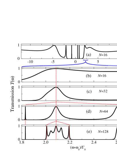
Figure 9: (Color online) Fine structure of the transmission spectra calculated for Thue-Morse quantum-well sequences of order $j=4,5,6,7$ ($N=16\ldots 128$). Calculated for $\Gamma=0$ and other parameters the same as in Fig. 1.

The transmission spectra are presented in Fig. 9 for different orders $j$ changing from $4$ ($N$ = 16 QWs) to $7$ ($N=128$). The spectrum has a complex structure with narrow peaks even for $N=16$, see Fig. 9(a). Figures 9(b)–9(d) show evolution of the spectra with increasing the number of QWs. The trace map (36b) alone is not sufficient to obtain transmission spectra. Therefore, to analyze the spectra we use the standard properties of the trace map (36b) and the antitrace maps Wang et al. (2000)

$$y_{j+1} =2x_{j-1}[(2x_{j}-1)y_{j-1}+\tilde{y}_{j-1}]\>,$$ (41)

$$\tilde{y}_{j+1} =2x_{j-1}[(2x_{j}-1)\tilde{y}_{j-1}+y_{j-1}]\>.$$

Here the half-antitrace $\tilde{y}_{j}$ corresponds to the structure $\widetilde{\mathcal{TM}}_{j}$ obtained from $\mathcal{TM}_{j}$ by the barrier interchange $\mathcal{A}\leftrightarrow\mathcal{B}$, e.g., $\mathcal{TM}_{2}=\mathcal{A}\mathcal{B}\mathcal{B}\mathcal{A}$ and $\widetilde{\mathcal{TM}}_{2}=\mathcal{B}\mathcal{A}\mathcal{A}\mathcal{B}$. Contrary to the Fibonacci case, the trace map (36b) for the Thue-Morse structures has no cycles of type (39). Instead of such cycles, Eqs. (36b) and (41) have the following property Ryu et al. (1993)

$$\text{if $x_{j-2}(\omega)=0$ then}\begin{cases}x_{j}(\omega)=x_{j+1}(\omega)=\ldots=1\>,\\ y_{j}(\omega)=y_{j+1}(\omega)=\ldots=0\>.\end{cases}$$ (42)

As a consequence, the structure becomes transparent at this particular frequency: $T_{j}(\omega)=T_{j+1}(\omega)=\ldots=1$. The positions of the spectral features follow then from Eq. (42). For example, the edges of the inner band gap for the Thue-Morse structure, $\omega_{L}=\omega_{0}-0.83\Gamma_{0}$ and $\omega_{R}=\omega_{0}+0.47\Gamma_{0}$, can be found from the equations $x_{1}(\omega_{L})=0$ and $x_{2}(\omega_{R})=0$, respectively.

Whenever the half-trace $x_{j-2}(\omega)$ vanishes at some frequency $\omega=\omega_{1}$ and therefore, $x_{j}(\omega_{1})=1$, there exist two neighboring frequencies, $\omega_{2}<\omega_{1}$ and $\omega_{3}>\omega_{1}$, such as $x_{j}(\omega_{2,3})=0$. As a consequence, $x_{j+2}(\omega_{2,3})=1$ and the transmission coefficient for the structure $\mathcal{TM}_{j+2}$ at these frequencies reaches unity. Thus the number of transmission peaks increases with the growth of the structure order: each unitary peak in the spectrum of the structure $\mathcal{TM}_{j}$ (i) persists in the spectra of the structures $\mathcal{TM}_{j+1},\mathcal{TM}_{j+2},\ldots$ of higher orders and (ii) leads to appearance of two more adjacent peaks for the structure $\mathcal{TM}_{j+2}$. An example of such “tree” of trifucations is indicated in Figs. 9(b)–9(e) by dashed lines. The single transmission peak of the structure $\mathcal{TM}_{4}$ ($N=16$) at $\omega\approx\omega_{0}+2.1\Gamma_{0}$ has generated the two peaks at $\omega\approx\omega_{0}+1.8\Gamma_{0}$ and $\omega\approx\omega_{0}+2.6\Gamma_{0}$ for the structure $\mathcal{TM}_{6}$ ($N=64$), cf. Fig. 9(b) and Fig. 9(d). The characteristic widths of the spectral features tend to zero proportional to a power the structure length $N_{j}^{-\alpha}=2^{-j\alpha}$, where $\alpha$ is a frequency-dependent positive index. Transmission spectra can also have non-unity maxima, see Fig. 9(e). These peaks do not correspond to any special values of $x_{j}$ and $y_{j}$ and their positions depend on $j$. The spatial distribution of the electric field on the frequencies with unitary transmission has a so-called “lattice-like” shape, specific for the Thue-Morse structures.Ryu et al. (1992)

The spectra presented in Fig. 9 are calculated for the Bragg structure with $q(\omega_{0})(a+b)=2\pi$. An interesting property of the Thue-Morse lattices, satisfying the Bragg condition $q(\omega_{0})(a+b)=\pi,2\pi\ldots$, is the mirror symmetry between the transmission spectra $T(\omega)$ and $\widetilde{T}(\omega)$, of the structures $\mathcal{TM}_{j}$ and $\widetilde{\mathcal{TM}}_{j}$, holding in the region $|\omega-\omega_{0}|\ll\sqrt{\Gamma_{0}\omega_{0}}$ in which case $q=q(\omega)$ in Eq. (33) can be approximated by $q(\omega_{0})$. The spectra are symmetrical with respect to $\omega=\omega_{0}$: $\widetilde{T}(\omega)=T(2\omega_{0}-\omega)$.

VI Conclusions

We have developed a theory of exciton-polaritons in photonic-quasicrystalline and aperiodic MQW structures having two different values of the interwell distances, $\mathcal{A}$ and $\mathcal{B}$. The approach based on the two-wave approximation has been extended to derive both the dispersion equation and analytical formulas for the reflectance and transmittance spectra from aperiodic MQW sequences. This approximation successfully describes the pattern of the optical spectra including the pair of stop-bands and interference fringes between them but stops being valid in a spectral range $|\omega-\omega_{0}|\sim\Gamma_{0}$ near the exciton resonant frequency $\omega_{0}$. In the Fibonacci QW chains with small values of the exciton nonradiative damping rate, $\Gamma<\Gamma_{0}$, the transmittance spectra and polariton band structure reveal, at two edges of the narrow inner band gap, a complicated and rich structure demonstrating scaling invariance and self-similarity. It has been shown that this structure can be related to the “band-edge” cycle of the trace map. The fine structure of optical spectra in the Thue-Morse MQWs can be interpreted in terms of zero reflection frequencies, or frequencies of unity transmittance.Ryu et al. (1993)

Appendix

Here we will analyze the second order of the perturbation theory at the point $K=-K^{\prime}=G_{h^{\vphantom{{}^{\prime}}}h^{\prime}}/2\equiv q_{0}$ and confirm the high accuracy of the stop-band edges defined by Eqs. (24).

We consider the terms in Eqs. (17) proportional to the structure-factor coefficients $f_{h-g,h^{\prime}-g^{\prime}}^{*}$ as a perturbation. Then keeping the second order contributions we obtain the following equations for the amplitudes $E_{K}$ and $E_{K^{\prime}}=E_{-K}$:

$$[q^{2}-K^{2}+\chi(1+\chi\bar{d}^{2}\zeta_{11})]E_{K}+\chi(f^{*}_{hh^{\prime}}+\chi\bar{d}^{2}\zeta_{12})E_{-K}=0\>,$$

$$\chi(f_{hh^{\prime}}+\chi\bar{d}^{2}\zeta_{21})E_{K}+[q^{2}-K^{2}+\chi(1+\chi\bar{d}^{2}\zeta_{22})]E_{-K}=0\>.$$ (A1)

Here $\chi=2q\xi=2q\Gamma_{0}/[\bar{d}(\omega_{0}-\omega+{\rm i}\Gamma)]$,

$$\zeta_{11}=\zeta_{22}=\frac{1}{\bar{d}^{2}}\!\sum\limits_{\begin{subarray}{c}(g,g^{\prime})\neq(h,h^{\prime})\\ (g,g^{\prime})\neq(0,0)\end{subarray}}\frac{|f_{gg^{\prime}}|^{2}}{(K-G_{gg^{\prime}})^{2}-K^{2}}\>,$$ (A2)

$$\zeta_{21}=\zeta_{12}^{*}=\frac{1}{\bar{d}^{2}}\!\sum\limits_{\begin{subarray}{c}(g,g^{\prime})\neq(h,h^{\prime})\\ (g,g^{\prime})\neq(0,0)\end{subarray}}\frac{f_{h-g,h^{\prime}-g^{\prime}}f_{gg^{\prime}}}{(K-G_{gg^{\prime}})^{2}-K^{2}}\>.$$ (A3)

We remind that, for the Fibonacci chains, the structure-factor coefficients are given by

$$f_{gg^{\prime}}=\frac{\sin S_{gg^{\prime}}}{S_{gg^{\prime}}}\exp\Bigl{(}{\rm i}\frac{\tau-2}{\tau}S_{gg^{\prime}}\Bigr{)},\quad S_{gg^{\prime}}=\frac{\pi\tau}{\tau^{2}+1}(\tau g^{\prime}-g)\>.$$ (A4)

The applied perturbation theory differs from the standard one by the presence of terms in the corresponding sums with the denominators $(K-G_{gg^{\prime}})^{2}-K^{2}$ arbitrarily close to zero. However the sums are finite because the smallness of the denominator at particular values of $g$ and $g^{\prime}$ is compensated by much smaller values of the numerators for the same values of $g,g^{\prime}$. The convergence of the sum (A2) for pairs $g,g^{\prime}$ where $G_{gg^{\prime}}\approx 0$ or $G_{gg^{\prime}}\approx G_{hh^{\prime}}$ is checked as follows. Taking into account the symmetry property $|f_{gg^{\prime}}|=|f_{-g,-g^{\prime}}|$ we can perform the following replacement in Eq. (A2)

$$\frac{|f_{gg^{\prime}}|^{2}}{(K-G_{gg^{\prime}})^{2}-K^{2}}\to\frac{|f_{gg^{\prime}}|^{2}}{G_{gg^{\prime}}^{2}-G^{2}_{hh^{\prime}}}\>.$$

Therefore, this sum converges for the pairs $g,g^{\prime}$ with $G_{gg^{\prime}}$ tending to zero. Now let us consider the sequence of pairs $(g,g^{\prime})=(h+k,h^{\prime}+k^{\prime})$, where

$$k=mF_{j},k^{\prime}=-mF_{j+1}\>,$$

$F_{j}$ are the Fibonacci numbers and $m$ is any integer $\pm 1,\pm 2...$ different from 0. Taking into account that

$$F_{j}=\frac{\tau^{j}-(1-\tau)^{j}}{2\tau-1}\>,\>\frac{F_{j}}{\tau}-F_{j-1}=\frac{(1-\tau)^{j-1}}{\tau}$$

the chosen sequence possesses the properties

$$G_{gg^{\prime}}-G_{hh^{\prime}}=-m\frac{2\pi}{\bar{d}}\frac{(1-\tau)^{j-1}}{\tau}\>,$$

$$S^{2}_{gg^{\prime}}(j\to\infty)\approx\left(\frac{\pi m\tau}{2\tau-1}\right)^{2}\tau^{2(j-1)}\ .$$

and, hence, with increasing $j$ one has

$$|G_{gg^{\prime}}-G_{hh^{\prime}}|S^{2}_{gg^{\prime}}\propto|m|^{3}\tau^{j}$$

which means that the sum

$$\sum\limits_{m,j}|G_{gg^{\prime}}-G_{hh^{\prime}}|^{-1}S^{-2}_{gg^{\prime}}$$

converges. The convergence in Eq. (A3) is checked in a similar way.

Numerical calculation performed for the Fibonacci QW chain with $(h,h^{\prime})=(1,0)$ shows that $|\zeta_{11}|$ and $|\zeta_{21}|$ are both smaller than $0.1$. The prefactor $\chi\bar{d}^{2}$ in Eq. (Appendix) is small as compared with $f_{hh^{\prime}}$ whenever

$${\rm max}\{|\omega_{0}-\omega|,\Gamma\}\gg\frac{2\pi\Gamma_{0}}{|f_{hh^{\prime}}|}\left(h+\frac{h^{\prime}}{\tau}\right)\>.$$ (A5)

We conclude that, for the wave (16) with $K=q_{0}$, the contributions from the wavevectors $G_{gg^{\prime}}$ different from 0 and $G_{hh^{\prime}}$ are negligible within the applicability range of Eq. (A5).

References

- Merlin et al. (1985) R. Merlin, K. Bajema, R. Clarke, F. Y. Juang, and P. K. Bhattacharya, Phys. Rev. Lett. 55, 1768 (1985).
- Kohmoto and Banavar (1986) M. Kohmoto and J. R. Banavar, Phys. Rev. B 34, 563 (1986).
- Ledermann et al. (2006) A. Ledermann, L. Cademartiri, M. Hermatschweiler, C. Toninelli, G. A. Ozin, D. S. Wiersma, M. Wegener, and G. von Freymann, Nature Materials 5, 942 (2006).
- Matsui et al. (2007) T. Matsui, A. Agrawal, A. Nahata, and Z. V. Vardeny, Nature 446, 517 (2007).
- Yablonovitch (1987) E. Yablonovitch, Phys. Rev. Lett. 58, 2059 (1987).
- John (1987) S. John, Phys. Rev. Lett. 58, 2486 (1987).
- Negro et al. (2004) L. D. Negro, M. Stolfi, Y. Yi, J. Michel, X. Duan, L. C. Kimerling, J. LeBlanc, and J. Haavisto, Appl. Phys. Lett. 84, 5186 (2004).
- Albuquerque and Cottam (2003) E. L. Albuquerque and M. G. Cottam, Phys. Rep. 376, 225 (2003).
- Passias et al. (2009) V. Passias, N. V. Valappil, Z. Shi, L. Deych, A. A. Lisyansky, and V. M. Menon, Opt. Express 17, 6636 (2009).
- Ivchenko et al. (1994) E. L. Ivchenko, A. I. Nesvizhskii, and S. Jorda, Phys. Solid State 36, 1156 (1994).
- Hübner et al. (1996) M. Hübner, J. Kuhl, T. Stroucken, A. Knorr, S. W. Koch, R. Hey, and K. Ploog, Phys. Rev. Lett. 76, 4199 (1996).
- Prineas et al. (2000) J. P. Prineas, C. Ell, E. S. Lee, G. Khitrova, H. M. Gibbs, and S. W. Koch, Phys. Rev. B 61, 13863 (2000).
- Pilozzi et al. (2004) L. Pilozzi, A. D’Andrea, and K. Cho, Phys. Rev. B 69, 205311 (2004).
- Ivchenko and Willander (1999) E. L. Ivchenko and M. Willander, phys. stal. sol. (b) 215, 199 (1999).
- Ivchenko et al. (2004) E. L. Ivchenko, M. M. Voronov, M. V. Erementchouk, L. I. Deych, and A. A. Lisyansky, Phys. Rev. B 70, 195106 (2004).
- Merle d’Aubigné et al. (1996) Y. Merle d’Aubigné, A. Wasiela, H. Mariette, and T. Dietl, Phys. Rev. B 54, 14003 (1996).
- Sadowski et al. (1997) J. Sadowski, H. Mariette, A. Wasiela, R. André, Y. Merle d’Aubigné, and T. Dietl, Phys. Rev. B 56, R1664 (1997).
- Haas et al. (1998) S. Haas, T. Stroucken, M. Hübner, J. Kuhl, B. Grote, A. Knorr, F. Jahnke, S. W. Koch, R. Hey, and K. Ploog, Phys. Rev. B 57, 14860 (1998).
- Hayes et al. (1999) G. R. Hayes, J. L. Staehli, U. Oesterle, B. Deveaud, R. T. Phillips, and C. Ciuti, Phys. Rev. Lett. 83, 2837 (1999).
- Deych and Lisyansky (2000) L. I. Deych and A. A. Lisyansky, Phys. Rev. B 62, 4242 (2000).
- Poddubny et al. (2008) A. N. Poddubny, L. Pilozzi, M. M. Voronov, and E. L. Ivchenko, Phys. Rev. B 77, 113306 (2008).
- Hendrickson et al. (2008) J. Hendrickson, B. C. Richards, J. Sweet, G. Khitrova, A. N. Poddubny, E. L. Ivchenko, M. Wegener, and H. M. Gibbs, Opt. Express 16, 15382 (2008).
- Werchner et al. (2009) M. Werchner, M. Schafer, M. Kira, S. W. Koch, J. Sweet, J. D. Olitzky, J. Hendrickson, B. C. Richards, G. Khitrova, H. M. Gibbs, et al., Opt. Express 17, 6813 (2009).
- Lin et al. (1995a) Z. Lin, H. Kubo, and M. Goda, Z. Phys. B: Cond. Matter 98, 111 (1995a).
- Azbel (1979) M. Y. Azbel, Phys. Rev. Lett. 43, 1954 (1979).
- Valsakumar and Kumar (1986) M. C. Valsakumar and V. Kumar, Pramana 26, 215 (1986).
- C.Janot (1994) C.Janot, Quasicrystals. A Primer (Clarendon Press, Oxford, UK, 1994).
- Fu et al. (1997) X. Fu, Y. Liu, P. Zhou, and W. Sritrakool, Phys. Rev. B 55, 2882 (1997).
- Luck et al. (1993) J. M. Luck, C. Godreche, A. Janner, and T. Janssen, J. Phys. A 26, 1951 (1993).
- Kolář (1993) M. Kolář, Phys. Rev. B 47, 5489 (1993).
- Kolář et al. (1993) M. Kolář, B. Iochum, and L. Raymond, J. Phys. A 26, 7343 (1993).
- Lin et al. (1995b) Z. Lin, M. Goda, and H. Kubo, J. Phys. A 28, 853 (1995b).
- Cheng et al. (1988) Z. Cheng, R. Savit, and R. Merlin, Phys. Rev. B 37, 4375 (1988).
- Liviotti (1996) E. Liviotti, Journ. of Phys.: Cond. Mat. 8, 5007 (1996).
- C.Kittel (1996) C.Kittel, Introduction to Solid State Physics (Wiley, New York, 1996).
- Ikawa and Cho (2002) T. Ikawa and K. Cho, Phys. Rev. B 66, 085338 (2002).
- Ivchenko (2005) E. L. Ivchenko, Optical spectroscopy of semiconductor nanostructures (Alpha Science International, Harrow, UK, 2005).
- Makhniy et al. (2006) V. Makhniy, M. Slyotov, V. Gorley, P. Horley, Y. Vorobiev, and J. González-Hernández, Appl. Surf. Sci. 253, 246 (2006).
- Kagan (1999) Y. Kagan, Hyperfine Interactions 123, 83 (1999).
- Ivchenko and Poddubny (2006) E. L. Ivchenko and A. N. Poddubny, Phys. Sol. State 48, 581 (2006).
- Brehm (1991) J. Brehm, Z. Phys. B: Cond. Matter 85, 145 (1991).
- Kolář and Ali (1990) M. Kolář and M. K. Ali, Phys. Rev. A 42, 7112 (1990).
- Kohmoto and Oono (1984) M. Kohmoto and Y. Oono, Phys. Lett. 102A, 145 (1984).
- Kohmoto et al. (1987) M. Kohmoto, B. Sutherland, and C. Tang, Phys. Rev. B 35, 1020 (1987).
- Zekri and Brezini (1992) N. Zekri and A. Brezini, phys. stat. sol. (b) 169, 253 (1992).
- Wang et al. (2000) X. Wang, U. Grimm, and M. Schreiber, Phys. Rev. B 62, 14020 (2000).
- Ryu et al. (1993) C. S. Ryu, G. Y. Oh, and M. H. Lee, Phys. Rev. B 48, 132 (1993).
- Ryu et al. (1992) C. S. Ryu, G. Y. Oh, and M. H. Lee, Phys. Rev. B 46, 5162 (1992).