Correlations for paths in
random orientations of $G(n,p)$ and $G(n,m)$

Abstract.

We study random graphs, both $G(n,p)$ and $G(n,m)$, with random orientations on the edges. For three fixed distinct vertices $s,a,b$ we study the correlation, in the combined probability space, of the events $\{a\to s\}$ and $\{s\to b\}$.

For $G(n,p)$, we prove that there is a $p_{\mathsf{c}}=1/2$ such that for a fixed $p<p_{\mathsf{c}}$ the correlation is negative for large enough $n$ and for $p>p_{\mathsf{c}}$ the correlation is positive for large enough $n$. We conjecture that for a fixed $n\geq 27$ the correlation changes sign three times for three critical values of $p$.

For $G(n,m)$ it is similarly proved that, with $p=m/\binom{n}{2}$, there is a critical $p_{\mathsf{c}}$ that is the solution to a certain equation and approximately equal to 0.7993. A lemma, which computes the probability of non existence of any $\ell$ directed edges in $G(n,m)$, is thought to be of independent interest.

We present exact recursions to compute $\operatorname{\mathbb{P}{}}(a\to s)$ and $\operatorname{\mathbb{P}{}}(a\to s,s\to b)$. We also briefly discuss the corresponding question in the quenched version of the problem.

1. Introduction

For a graph $G=(V,E)$ we orient each edge with equal probability for the two possible directions and independent of all other edges. This model has been studied previously in for instance [1, 6, 12]. Let $s,a,b$ be fixed distinct vertices in the graph. Let $\{a\to s\}$ denote the event that there exists a directed path from $a$ to $s$. The object of this paper is to study the correlation of the two events $\{a\to s\}$ and $\{s\to b\}$ in a random graph. One might intuitively guess that they are negatively correlated in any graph, that is $\operatorname{\mathbb{P}{}}(a\to s,s\to b)-\operatorname{\mathbb{P}{}}(a\to s)\operatorname{\mathbb{P}{}}(s\to b)<0$. This is however not true for all graphs. In fact, the smallest counter example is the graph on four vertices with all edges except $\{a,b\}$. In [1] it was proved that for the complete graph $K_{n}$ they are negatively correlated for $n=3$, independent for $n=4$ and positively correlated for $n\geq 5$. The results in [1] suggested that the correlation seemed more likely to be positive in dense graphs, which led us to further investigate the correlation in $G(n,p)$ and in $G(n,m)$ as presented in the present paper.

There are two different ways of combining the two random processes. In this paper we deal with the annealed case, which means that we consider the joined probability space of $G(n,p)$ (or $G(n,m)$) and that of edge orientations. We then consider correlations of events in this space. The other possibility is the quenched version, in which one for each graph in $G(n,p)$ (or $G(n,m)$) computes the correlation of the two events in the probability space of all edge orientations in that graph. Then one takes the expected value over all graphs. We discuss briefly the quenched version in Section 9.

In the random graph $G(n,p)$ there are $n$ vertices and every edge exists with probability $p$, $0\leq p\leq 1$, independently of other edges. Let ${\vec{G}(n,p)}$ be a directed graph obtained by giving each edge in $G(n,p)$ a random direction. Our main result in Section 2 implies that for a fixed $p$ the events are positively correlated when $p>1/2$ for large enough $n$, but negatively correlated when $p<1/2$ for large enough $n$. To be more precise, in Theorem 2.1 we prove that

$$\frac{\operatorname{\mathbb{P}{}}(a\mathrel{\not\to}s,s\mathrel{\not\to}b)-\operatorname{\mathbb{P}{}}(a\mathrel{\not\to}s)\operatorname{\mathbb{P}{}}(s\mathrel{\not\to}b)}{\operatorname{\mathbb{P}{}}(a\mathrel{\not\to}s,s\mathrel{\not\to}b)}\to\frac{2p-1}{3}\text{ as }n\to\infty.$$

Note that the covariance is bilinear so that $\operatorname{\mathbb{P}{}}(a\to s,s\to b)-\operatorname{\mathbb{P}{}}(a\to s)\operatorname{\mathbb{P}{}}(s\to b)=\operatorname{\mathbb{P}{}}(a\mathrel{\not\to}s,s\mathrel{\not\to}b)-\operatorname{\mathbb{P}{}}(a\mathrel{\not\to}s)\operatorname{\mathbb{P}{}}(s\mathrel{\not\to}b)$. Thus we may instead study the complementary events $\{a\mathrel{\not\to}s\}$, that there does not exist a directed path from $a$ to $s$, and $\{s\mathrel{\not\to}b\}$, which turns out to be more practical. The change of sign for the correlation at $p=1/2$ was unexpected for us. An attempt to an heuristic explanation is given just after the statement of Theorem 2.1.

In Section 5 we give exact recursions for the probabilities $\operatorname{\mathbb{P}{}}(a\mathrel{\not\to}s),\operatorname{\mathbb{P}{}}(s\mathrel{\not\to}b)$ and $\operatorname{\mathbb{P}{}}(a\mathrel{\not\to}s,s\mathrel{\not\to}b)$. This is done by studying the size of the set of the vertices that can be reached along a directed path from a given vertex $s$ and the size of the set of vertices from which there is a directed path to $s$. We give recursions for the joint distribution of these sizes, which could be of independent interest.

The situation seems however to be much more complicated than what is suggested by Theorem 2.1. In Section 6 we report our results from exact computations using the recursions. It turns out that for $n\geq 27$ the difference $\operatorname{\mathbb{P}{}}(a\to s,s\to b)-\operatorname{\mathbb{P}{}}(a\to s)\cdot\operatorname{\mathbb{P}{}}(s\to b)$ seems to change sign three times. First twice for small $p$ (roughly $constant/n$) and then it goes from negative to positive again just before $p=1/2$. We find this behavior mysterious but conjecture it to be true in general and plan to study this further in a coming paper.

For $0\leq m\leq\binom{n}{2}$, $G(n,m)$ is the random graph with $n$ vertices (which we take as $1,\dots,n$) and $m$ edges, uniformly chosen among all such graphs. We let ${\vec{G}(n,m)}$ be the directed random graph obtained from $G(n,m)$ by giving each edge a random direction. It is less straightforward to study the probabilities in ${\vec{G}(n,m)}$, but thanks to Lemma 3.2, we can prove the corresponding statement for ${\vec{G}(n,m)}$ in parallel with the proof for ${\vec{G}(n,p)}$. Here the critical probability is $\approx 0.799288221$, see Theorem 2.2. The exact computations and the simulations for ${\vec{G}(n,m)}$ do not give reason to believe that there is more than one critical probability for a fixed $n$. It might be consternating that ${\vec{G}(n,m)}$ and ${\vec{G}(n,p)}$ behave so differently. In Section 8 we explain this and prove that the correlation in ${\vec{G}(n,p)}$ is always larger, in a certain sense, than in ${\vec{G}(n,m)}$. The difference is expressed as a variance for which we give an exact asymptotic expression, see Theorem 8.2.

The background of the questions studied in this paper is as follows. Let $G$ be any graph and $a,b,s,t$ distinct vertices of $G$. Further, assign a random orientation to the graph as described above, that is each edge is given its direction independent of the other edges. In [12] it was proved that then the events $\{s\to a\}$ and $\{s\to b\}$ are positively correlated. This was shown to be true also if we first conditioned on $\{s\mathrel{\not\to}t\}$, i.e. $\operatorname{\mathbb{P}{}}(s\to a,s\to b\mid s\mathrel{\not\to}t)\geq\operatorname{\mathbb{P}{}}(s\to a\mid s\mathrel{\not\to}t)\cdot\operatorname{\mathbb{P}{}}(s\to b\mid s\mathrel{\not\to}t)$. Note that it is not intuitively clear why this is so. It is for instance no longer true if we instead condition on $\{s\to t\}$. In another direction, it was proved that $\operatorname{\mathbb{P}{}}(s\to b,a\to t\mid s\mathrel{\not\to}t)\leq\operatorname{\mathbb{P}{}}(s\to b\mid s\mathrel{\not\to}t)\cdot\operatorname{\mathbb{P}{}}(a\to t\mid s\mathrel{\not\to}t)$. The proofs in [12] relied heavily on the results in [5] and [4] where similar statements were proved for edge percolation on a given graph. These questions have to a large extent been inspired by an interesting conjecture due to Kasteleyn named the Bunkbed conjecture by Häggström [8], see also [11] and Remark 5 in [5].

Acknowledgment: We thank the anonymous referees for very helpful comments.

2. Main Theorems

Let $G(n,p)$ be the random graph where each edge has probability $p$ of being present independent of other edges. We further orient each present edge either way independently with probability $\frac{1}{2}$ and call the resulting random directed graph ${\vec{G}(n,p)}$. It turns out to be convenient to study the negated events $\{a\mathrel{\not\to}s\}$ and $\{s\mathrel{\not\to}b\}$. We say that two events $A$ and $B$ are negatively correlated if

$$\operatorname{Cov}(A,B):=\operatorname{\mathbb{P}{}}(A\cap B)-\operatorname{\mathbb{P}{}}(A)\operatorname{\mathbb{P}{}}(B)<0,$$

and positively correlated if the inequality goes the other way. If $A$ and $B$ are negatively correlated, then $A$ and $\neg B$ are positively correlated. Thus $a\mathrel{\not\to}s$ and $s\mathrel{\not\to}b$ are negatively correlated if and only if $\{a\to s\}$ and $\{s\to b\}$ are negatively correlated. Trivially, $\operatorname{\mathbb{P}{}}(a\mathrel{\not\to}s)=\operatorname{\mathbb{P}{}}(s\mathrel{\not\to}b)$.

All unspecified limits are as ${n\to\infty}$.

The case $p=1$ corresponds to random orientations of the complete graph $K_{n}$. In [1] it was proved that $a\mathrel{\not\to}s$ and $s\mathrel{\not\to}b$ are negatively correlated in $K_{3}$, independent in $K_{4}$ and positively correlated in $K_{n}$ for $n\geq 5$. It was in fact proved that the relative covariance $(\operatorname{\mathbb{P}{}}(a\mathrel{\not\to}s,s\mathrel{\not\to}b)-\operatorname{\mathbb{P}{}}(a\mathrel{\not\to}s)\operatorname{\mathbb{P}{}}(s\mathrel{\not\to}b))/\operatorname{\mathbb{P}{}}(a\mathrel{\not\to}s,s\mathrel{\not\to}b)$ converged to $\frac{1}{3}$ as $n\to\infty$.

For ${\vec{G}(n,p)}$ our main theorem is as follows.

Theorem 2.1.

For a fixed $p\in(0,1]$ and fixed distinct vertices $a,b,s\in{\vec{G}(n,p)}$ we have the following limit of the relative covariance

$$\lim_{n\to\infty}\frac{\operatorname{\mathbb{P}{}}(a\mathrel{\not\to}s,s\mathrel{\not\to}b)-\operatorname{\mathbb{P}{}}(a\mathrel{\not\to}s)\operatorname{\mathbb{P}{}}(s\mathrel{\not\to}b)}{\operatorname{\mathbb{P}{}}(a\mathrel{\not\to}s,s\mathrel{\not\to}b)}=\frac{2p-1}{3}.$$

In particular, for large enough $n$:

1. If $0<p<1/2$, then $\operatorname{Cov}(s\mathrel{\not\to}a,\,b\mathrel{\not\to}s)<0$.

2. If $1/2<p\leq 1$, then $\operatorname{Cov}(s\mathrel{\not\to}a,\,b\mathrel{\not\to}s)>0$.

Furthermore,

$$\operatorname{Cov}(s\mathrel{\not\to}a,\,b\mathrel{\not\to}s)=(2p-1+o(1))(1-p/2)^{2n-3}.$$ (1)

One way to heuristically understand the critical probability $1/2$ is as follows. For the event $\{s\mathrel{\not\to}a\}$ the two cases that dominate for large $n$ are $i)$ no edge points out from $s$ and $ii)$ no edge points in to $a$, each with probability $(1-p/2)^{n-1}$. Similarly for $\{b\mathrel{\not\to}s\}$. Thus $\operatorname{\mathbb{P}{}}(s\mathrel{\not\to}a)\operatorname{\mathbb{P}{}}(b\mathrel{\not\to}s)$ is roughly $4\cdot(1-p/2)^{2n-2}$. For the joint probability $\operatorname{\mathbb{P}{}}(s\mathrel{\not\to}a,b\mathrel{\not\to}s)$ on the other hand, we only need to consider three of these cases since no edges at all around $s$ has a much smaller probability. This gives a negative contribution to the covariance and is perhaps the most striking contribution. But, the other three cases have in the joint probability a factor $1-p/2$ less since one edge is common, which gives a positive contribution. Thus the quotient $\frac{\operatorname{\mathbb{P}{}}(s\mathrel{\not\to}a,b\mathrel{\not\to}s)}{\operatorname{\mathbb{P}{}}(s\mathrel{\not\to}a)\operatorname{\mathbb{P}{}}(b\mathrel{\not\to}s)}\sim\frac{3/4}{1-p/2}$, which is greater than 1 if and only if $p>1/2$.

Theorem 2.1 was proved in an earlier version of this manuscript, see [2], with a rather lengthy calculation to estimate the involved probabilities. In the present version we will present a shorter proof which also has the advantage that it allows us to prove the covariance also in ${\vec{G}(n,m)}$. However, we want to point out that the lengthy calculations in [2] could be shortened with a clever lemma by Backelin, see [3].

For ${\vec{G}(n,m)}$, we obtain the corresponding result.

Theorem 2.2.

Suppose that $m,n\to\infty$, and that $m/\binom{n}{2}\to p\in(0,1]$. Let $p_{\mathsf{c}}\approx 0.799$ be the unique root in $[0,1]$ of $3e^{-\frac{2p(1-p)}{(2-p)^{2}}}=4-2p$. If $n$ is large enough, then for any distinct vertices $s,a,b\in{\vec{G}(n,m)}$:

1. If $0<p<p_{\mathsf{c}}$, then $\operatorname{Cov}(s\mathrel{\not\to}a,\,b\mathrel{\not\to}s)<0$.

2. If $p_{\mathsf{c}}<p\leq 1$, then $\operatorname{Cov}(s\mathrel{\not\to}a,\,b\mathrel{\not\to}s)>0$.

In fact we have the following asymptotic formula for the covariance.

Theorem 2.3.

Suppose that $m,n\to\infty$, let $p=p(n):=m/\binom{n}{2}$, and assume $\liminf p(n)>0$. Then, for any distinct vertices $s,a,b\in{\vec{G}(n,m)}$:

$$\operatorname{Cov}(s\mathrel{\not\to}a,\,b\mathrel{\not\to}s)=\left(\frac{3}{4-2p}e^{-\frac{2p(1-p)}{(2-p)^{2}}}-1+o(1)\right)\operatorname{\mathbb{P}{}}(s\mathrel{\not\to}a)^{2}\\ =\left(3\cdot e^{-\frac{2p(1-p)}{(2-p)^{2}}}-4+2p+o(1)\right)\cdot(1-p/2)^{2n-3}\cdot e^{-\frac{2p(1-p)}{(2-p)^{2}}}.$$

3. Two lemmas

In order to prove the theorems for ${\vec{G}(n,p)}$ and ${\vec{G}(n,m)}$ in parallel we need two lemmas.

Lemma 3.1.

Fix $\ell\geq 0$ edges in $K_{n}$. The probability that none of these $\ell$ edges appears in $G(n,m)$ is at most $\left(1-m/\binom{n}{2}\right)^{\ell}$.

Proof.

Let $N:=\binom{n}{2}$. We may assume that $m+\ell\leq N$. Then the probability is

$$\frac{\binom{N-\ell}{m}}{\binom{N}{m}}=\frac{(N-\ell)!\,(N-m)!}{(N-\ell-m)!\,N!}=\prod_{i=0}^{\ell-1}\frac{N-m-i}{N-i}\leq\prod_{i=0}^{\ell-1}\Bigl{(}1-\frac{m}{N}\Bigr{)}.\qed$$

Note that in $G(n,p)$ the corresponding probability is exactly $(1-p)^{\ell}$ by independence of the edges. We next show a more precise version of Lemma 3.1 for the directed graph $\vec{G}(n,m)$.

Let $q(\ell)=q(\ell;n,m)$ be the probability that if we fix $\ell$ edges in $K_{n}$ and give each an orientation, then none of these directed edges appears in $\vec{G}(n,m)$. (Here $0\leq\ell\leq\binom{n}{2}$. By symmetry, the probability does not depend on the choice of the $\ell$ edges and their orientations.) Let also $q^{\prime}(\ell;n,p)$ be the corresponding probability in ${\vec{G}(n,p)}$. It is clear that $q^{\prime}(\ell;n,p)=(1-p/2)^{\ell}$. For ${\vec{G}(n,m)}$ we have the following result, which we believe is of independent interest.

Lemma 3.2.

Suppose that $\ell=\ell(n)=O(n)$ and that $0\leq m=m(n)\leq\binom{n}{2}$. Then, with $p=p(n)=m(n)/\binom{n}{2}$, as ${n\to\infty}$,

$$q(\ell;n,m)\sim(1-p/2)^{\ell}\exp\left(-\Bigl{(}\frac{\ell}{n}\Bigr{)}^{2}\frac{p(1-p)}{(2-p)^{2}}\right).$$ (2)

Furthermore, for any $\ell,n,m$ we have $q(\ell;n,m)\leq q^{\prime}(\ell;n,p)=(1-p/2)^{\ell}$.

Proof.

Let $N:=\binom{n}{2}$. The cases $m=0$ and $m=N$ are trivial, so we may assume that $0<m<N$ and thus $0<p<1$.

Let $X$ be the number of the $\ell$ chosen edges that appear in $G(n,m)$, ignoring orientations. Then $X$ has the hypergeometric distribution

$$\operatorname{\mathbb{P}{}}(X=k)=\frac{\binom{\ell}{k}\binom{N-\ell}{m-k}}{\binom{N}{m}}=\binom{\ell}{k}\frac{(N-\ell)!\,(N-m)!\,m!}{N!\,(N-m-\ell+k)!\,(m-k)!}.$$ (3)

Define, for $J,j\geq 0$, $a(J,j):=J^{-j}J!/(J-j)!$ (interpreted as 0 when $j>J$). Then (3) can be written as

$$\begin{split}\operatorname{\mathbb{P}{}}(X=k)&=\binom{\ell}{k}a(N,\ell)^{-1}N^{-\ell}a(N-m,\ell-k)(N-m)^{\ell-k}a(m,k)m^{k}\\ &=\binom{\ell}{k}p^{k}(1-p)^{\ell-k}a(N,\ell)^{-1}a(N-m,\ell-k)a(m,k).\end{split}$$

Given $X=k$, the probability that none of the selected directed edges appears in ${\vec{G}(n,m)}$ equals the probability that none of the $k$ selected edges that appear in $G(n,m)$ gets the forbidden orientation, which equals $(1/2)^{k}$. Hence,

$$\begin{split}q(\ell)&=\sum_{k=0}^{\ell}2^{-k}\operatorname{\mathbb{P}{}}(X=k)\\ &=\sum_{k=0}^{\ell}\binom{\ell}{k}\Bigl{(}\frac{p}{2}\Bigr{)}^{k}(1-p)^{\ell-k}a(N,\ell)^{-1}a(N-m,\ell-k)a(m,k)\\ &=a(N,\ell)^{-1}(1-p/2)^{\ell}\sum_{k=0}^{\ell}\binom{\ell}{k}\Bigl{(}\frac{p/2}{1-p/2}\Bigr{)}^{k}\Bigl{(}1-\frac{p/2}{1-p/2}\Bigr{)}^{\ell-k}a(N-m,\ell-k)a(m,k)\\ &=a(N,\ell)^{-1}(1-p/2)^{\ell}\operatorname{\mathbb{E}{}}\bigl{(}a(m,Y)a(N-m,\ell-Y)\bigr{)},\end{split}$$

where $Y$ has the binomial distribution $\operatorname{Bin}(\ell,p/(2-p))$. Consequently, (2) is equivalent to

$$a(N,\ell)^{-1}\operatorname{\mathbb{E}{}}\bigl{(}a(m,Y)a(N-m,\ell-Y)\bigr{)}\sim\exp\left(-\Bigl{(}\frac{\ell}{n}\Bigr{)}^{2}\frac{p(1-p)}{(2-p)^{2}}\right).$$ (4)

In order to show (4), it suffices to show that every subsequence has a subsequence where (4) holds. (See [10, p. 12].) Consequently, by choosing suitable subsequences, we may assume that

$$\ell/n\to\lambda\qquad\text{and}\qquad p\to\pi,$$ (5)

for some $\lambda\in[0,\infty)$ and $\pi\in[0,1]$; furthermore, we may assume that either

$$\ell\to\infty\qquad\text{or}\qquad l=O(1).$$ (6)

We next observe that for all $J\geq 1$ and $j\leq J$,

$$a(J,j)=J^{-j}\prod_{i=0}^{j-1}(J-i)=\prod_{i=0}^{j-1}\Bigl{(}1-\frac{i}{J}\Bigr{)}=\exp\left(\sum_{i=1}^{j-1}\log\Bigl{(}1-\frac{i}{J}\Bigr{)}\right).$$

It follows that $0\leq a(j,J)\leq 1$ for all $j$ and $J$. Moreover, if $j=O(J^{1/2})$, then, if also $j\leq J$,

$$\begin{split}{\sum_{i=1}^{j-1}\log\Bigl{(}1-\frac{i}{J}\Bigr{)}}&=\sum_{i=1}^{j-1}\left(-\frac{i}{J}+O\Bigl{(}\frac{i}{J}\Bigr{)}^{2}\right)=-\frac{j^{2}-j}{2J}+O\Bigl{(}\frac{j^{3}}{J^{2}}\Bigr{)}\\ &=-\frac{j^{2}}{2J}+O\bigl{(}J^{-1/2}\bigr{)}\end{split}$$

and thus (also in the trivial case $j>J$)

$$a(J,j)=\exp\Bigl{(}-\frac{j^{2}}{2J}\Bigr{)}+O\bigl{(}J^{-1/2}\bigr{)}.$$ (7)

In particular, (7) applies to $a(N,\ell)$, because $\ell=O(n)=O(N^{1/2})$, and thus

$$a(N,\ell)=\exp\bigl{(}-\ell^{2}/2N\bigr{)}+o(1)\to\exp\bigl{(}-\lambda^{2}\bigr{)},$$ (8)

assuming (5).

Next, consider $a(m,Y)$, assuming (5)–(6). Assume first $\pi>0$. If also $\ell\to\infty$, then by the law of large numbers, $Y/\ell\overset{\mathrm{p}}{\longrightarrow}\pi/(2-\pi)$, and thus

$$\frac{Y^{2}}{2m}=\Bigl{(}\frac{Y}{\ell}\Bigr{)}^{2}\Bigl{(}\frac{\ell}{n}\Bigr{)}^{2}\cdot\frac{n^{2}/2}{m}\overset{\mathrm{p}}{\longrightarrow}\Bigl{(}\frac{\pi}{2-\pi}\Bigr{)}^{2}\lambda^{2}\frac{1}{\pi}=\frac{\pi}{(2-\pi)^{2}}\lambda^{2}.$$ (9)

On the other hand, if $\ell=O(1)$, then $\lambda=0$; furthermore, $Y\leq\ell=O(1)$ and $m\to\infty$ (because $\pi>0$), so $Y^{2}/2m\overset{\mathrm{p}}{\longrightarrow}0$; hence (9) holds in this case too.

In the case $\pi=0$, so $p\to 0$, we instead use

$$\operatorname{\mathbb{E}{}}Y=\ell p/(2-p)\leq p\ell=o\bigl{(}p^{1/2}\ell\bigr{)},$$

and thus $Y/(p^{1/2}\ell)\overset{\mathrm{p}}{\longrightarrow}0$. Hence,

$$\frac{Y^{2}}{2m}=\left(\frac{Y}{p^{1/2}\ell}\right)^{2}\cdot\frac{p\ell^{2}}{2m}=\left(\frac{Y}{p^{1/2}\ell}\right)^{2}\cdot\frac{\ell^{2}}{n(n-1)}\overset{\mathrm{p}}{\longrightarrow}0=\frac{\pi}{(2-\pi)^{2}}\lambda^{2},$$

so (9) holds in this case too.

Consequently, (9) holds in every case. In particular, $Y=O_{\mathrm{p}}(m^{1/2})$, and (7) implies that, provided $m\to\infty$,

$$a(m,Y)=\exp\left(-\frac{Y^{2}}{2m}\right)+o_{\mathrm{p}}(1)\overset{\mathrm{p}}{\longrightarrow}\exp\left(-\frac{\pi}{(2-\pi)^{2}}\lambda^{2}\right);$$ (10)

on the other hand, if $m=O(1)$, then $\operatorname{\mathbb{P}{}}(Y=0)\to 1$, e.g. by (9), so (10) holds in this case too. Consequently, (10) holds in every case.

Since $\ell-Y\sim\operatorname{Bin}\bigl{(}\ell,1-p/(2-p)\bigr{)}=\operatorname{Bin}(\ell,2(1-p)/(2-p))$, it follows by similar arguments, now considering the case $\pi=1$ separately, that

$$\frac{(\ell-Y)^{2}}{2(N-m)}\overset{\mathrm{p}}{\longrightarrow}\frac{4(1-\pi)}{(2-\pi)^{2}}\lambda^{2}$$

and

$$a(N-m,\ell-Y)\overset{\mathrm{p}}{\longrightarrow}\exp\left(-\frac{4(1-\pi)}{(2-\pi)^{2}}\lambda^{2}\right).$$ (11)

Combining (10) and (11) we find

$$a(m,Y)a(N-m,\ell-Y)\overset{\mathrm{p}}{\longrightarrow}\exp\left(-\frac{\lambda^{2}}{(2-\pi)^{2}}\bigl{(}\pi+4(1-\pi)\bigr{)}\right).$$

By dominated convergence, using $0\leq a(m,Y)a(N-m,\ell-Y)\leq 1$, this, together with (8), yields

$$\begin{split}a(N,\ell)^{-1}\operatorname{\mathbb{E}{}}\bigl{(}a(m,Y)a(N-m,\ell-Y)\bigr{)}&\to\exp\left(\lambda^{2}-\frac{\lambda^{2}}{(2-\pi)^{2}}(4-3\pi)\right)\\ =\exp\left(\frac{\lambda^{2}}{(2-\pi)^{2}}(\pi^{2}-\pi)\right),\end{split}$$

which is equivalent to (4) by (5). Hence (4) holds assuming (5)–(6), and thus in general, which shows (2).

Finally, let $X^{\prime}\sim\operatorname{Bin}(\ell,p)$ be the number of the $\ell$ chosen edges that appear in $G(n,p)$, ignoring orientations. Then, $q(\ell)=\operatorname{\mathbb{E}{}}{(\frac{1}{2})^{X}}$ as shown above, and similarly $q^{\prime}(\ell)=\operatorname{\mathbb{E}{}}{(\frac{1}{2})^{X^{\prime}}}$. In fact, $\operatorname{\mathbb{E}{}}a^{X}\leq\operatorname{\mathbb{E}{}}a^{X^{\prime}}$ for any $a>0$, see Hoeffding [9, Theorem 4], which, taking $a=1/2$, yields $q(\ell)\leq q^{\prime}(\ell)$. ∎

4. Proofs

Say that a set $S\subseteq V(G)$ of vertices in a directed graph $G$ is an outset if there is no directed edge $vw$ with $v\notin S$, $w\in S$ (i.e., all edges between $S$ and its complement are directed out from $S$), and an inset if there is no directed edge $vw$ with $v\in S$, $w\notin S$. Hence, $S$ is an outset if and only if its complement is an inset.

Lemma 4.1.

If $G$ is a directed graph and $a,b\in V(G)$, then the following are equivalent:

1. $a\mathrel{\not\to}b$.

2. There exists an inset $S$ with $a\in S$, $b\notin S$.

3. There exists an outset $T$ with $a\notin T$, $b\in T$.

Proof.

(i)$\iff$(ii): No directed path can leave an inset. Hence, if an inset $S$ as in (ii) exists, then $a\mathrel{\not\to}b$. Conversely, if $a\mathrel{\not\to}b$, then $S:=\{v\in V(G):a\to v\}$ is an inset with $a\in S$, $b\notin S$.

(ii)$\iff$(iii): Take $T:=V(G)\setminus S$, and conversely. ∎

For $S\subseteq[n]$, let $\mathcal{O}_{S}$ and $\mathcal{I}_{S}$ denote the events $\{S\text{ is an outset}\}$ and $\{S\text{ is an inset}\}$, respectively. The events will be in ${\vec{G}(n,m)}$ or ${\vec{G}(n,p)}$ depending on context. We also write, for typographical convenience, $\mathcal{O}_{a}:=\mathcal{O}_{\{a\}}$, etc.

Lemma 4.2.

Assume that $p\in(0,1]$ is fixed. Then, for any distinct $s,a\in{\vec{G}(n,p)}$,

$$\operatorname{\mathbb{P}{}}(s\mathrel{\not\to}a) =\operatorname{\mathbb{P}{}}(\mathcal{I}_{s})+\operatorname{\mathbb{P}{}}(\mathcal{O}_{a})+O\bigl{(}n(1-p/2)^{2n}\bigr{)}$$

$$=2q^{\prime}(n-1)+O\bigl{(}n(1-p/2)^{2n}\bigr{)}$$

$$\sim 2(1-p/2)^{n-1}.$$

The proof of Lemma 4.2 is very similar to the proof of Lemma 4.3 below, but with $q(\ell;n,m)$ replaced by $q^{\prime}(\ell;n,p)$.

Lemma 4.3.

Suppose that $m,n\to\infty$, let $p=p(n):=m/\binom{n}{2}$, and assume $\liminf p(n)>0$. Then, for any distinct $s,a\in{\vec{G}(n,m)}$,

$$\operatorname{\mathbb{P}{}}(s\mathrel{\not\to}a) =\operatorname{\mathbb{P}{}}(\mathcal{I}_{s})+\operatorname{\mathbb{P}{}}(\mathcal{O}_{a})+O\bigl{(}n(1-p/2)^{2n}\bigr{)}$$

$$=2q(n-1)+O\bigl{(}n(1-p/2)^{2n}\bigr{)}$$

$$\sim 2(1-p/2)^{n-1}e^{-\frac{p(1-p)}{(2-p)^{2}}}.$$

Proof.

Let $\mathcal{E}_{k}$ be the event that there exists an inset $S$ with $s\in S$, $a\notin S$ and $|S|=k$. Then, by Lemma 4.1,

$$\{s\mathrel{\not\to}a\}=\bigcup_{k=1}^{n-1}\mathcal{E}_{k}=\mathcal{E}_{1}\cup\mathcal{E}_{n-1}\cup\bigcup_{k=2}^{n-2}\mathcal{E}_{k}.$$ (12)

Here $\mathcal{E}_{1}=\mathcal{I}_{s}$ and $\mathcal{E}_{n-1}=\mathcal{O}_{a}$.

If $|S|=k$, then $\operatorname{\mathbb{P}{}}(\mathcal{I}_{S})=\operatorname{\mathbb{P}{}}(\mathcal{O}_{S})=q(k(n-k))$. In particular, by Lemma 3.2,

$$\operatorname{\mathbb{P}{}}(\mathcal{I}_{s})=\operatorname{\mathbb{P}{}}(\mathcal{O}_{a})=q(n-1)\sim(1-p/2)^{n-1}e^{-\frac{p(1-p)}{(2-p)^{2}}}.$$ (13)

Further, for any $k$, there are $\binom{n-2}{k-1}$ sets $S$ with $s\in S$, $a\notin S$ and $|S|=k$, and thus

$$\operatorname{\mathbb{P}{}}(\mathcal{E}_{k})\leq\binom{n-2}{k-1}q(k(n-k))\leq{n}^{k-1}q(k(n-k)).$$ (14)

For fixed $k$ we may apply Lemma 3.2 and obtain

$$\operatorname{\mathbb{P}{}}(\mathcal{E}_{k})=\operatorname{\mathbb{P}{}}(\mathcal{E}_{n-k})=O\bigl{(}{n}^{k-1}(1-p/2)^{k(n-k)}\bigr{)}=O\bigl{(}{n}^{k-1}(1-p/2)^{kn}\bigr{)}.$$ (15)

For a fixed $K$, we use this estimate for $k<K$. For $K\leq k\leq n-K$ we have $k(n-k)\geq K(n-K)$ and thus $q(k(n-k))\leq q(K(n-K))$, while the total number of subsets $S$ of $[n]$ is $2^{n}$, and thus Lemma 3.2 again yields

$$\operatorname{\mathbb{P}{}}\Bigl{(}\bigcup_{k=K}^{n-K}\mathcal{E}_{k}\Bigr{)}\leq 2^{n}q(K(n-K))=O\bigl{(}2^{n}(1-p/2)^{Kn}\bigr{)}.$$ (16)

By the assumption $\liminf p(n)>0$, we may assume that $p=p(n)\geq p_{0}$ for some $p_{0}>0$. Choosing $K$ such that $(1-p_{0}/2)^{K-2}\leq 1/2$, we have $2(1-p/2)^{K}\leq 2(1-p_{0}/2)^{K-2}(1-p/2)^{2}\leq(1-p/2)^{2}$, and thus (15) and (16) imply

$$\operatorname{\mathbb{P}{}}\Bigl{(}\bigcup_{k=2}^{n-2}\mathcal{E}_{k}\Bigr{)}=\sum_{k=2}^{K-1}O\bigl{(}n^{k-1}(1-p/2)^{kn}\bigr{)}+O\bigl{(}(1-p/2)^{2n}\bigr{)}=O\bigl{(}n(1-p/2)^{2n}\bigr{)}.$$

Hence, (12) yields

$$\operatorname{\mathbb{P}{}}\{s\mathrel{\not\to}a\}=\operatorname{\mathbb{P}{}}(\mathcal{E}_{1}\cup\mathcal{E}_{n-1})+O\bigl{(}n(1-p/2)^{2n}\bigr{)}=\operatorname{\mathbb{P}{}}(\mathcal{I}_{s}\cup\mathcal{O}_{a})+O\bigl{(}n(1-p/2)^{2n}\bigr{)}.$$ (17)

Finally, $\operatorname{\mathbb{P}{}}(\mathcal{I}_{s}\cap\mathcal{O}_{a})=q(2n-3)=O\bigl{(}(1-p/2)^{2n}\bigr{)}$ by Lemma 3.2 again, and thus $\operatorname{\mathbb{P}{}}(\mathcal{I}_{s}\cup\mathcal{O}_{a})=\operatorname{\mathbb{P}{}}(\mathcal{I}_{s})+\operatorname{\mathbb{P}{}}(\mathcal{O}_{a})+O\bigl{(}(1-p/2)^{2n}\bigr{)}$. The result now follows by (17) and (13). ∎

Lemma 4.4.

Suppose that $p\in(0,1]$ is fixed, then for any distinct $s,a,b\in{\vec{G}(n,p)}$,

$$\operatorname{\mathbb{P}{}}(s\mathrel{\not\to}a \text{ and }b\mathrel{\not\to}s)$$

$$=\operatorname{\mathbb{P}{}}(\mathcal{I}_{s,b}\cap\mathcal{I}_{b})+\operatorname{\mathbb{P}{}}(\mathcal{O}_{s,a}\cap\mathcal{O}_{a})+\operatorname{\mathbb{P}{}}(\mathcal{O}_{a}\cap\mathcal{I}_{b})+o\bigl{(}(1-p/2)^{2n}\bigr{)}$$

$$=3(1-p/2)^{2n-3}+o\bigl{(}(1-p/2)^{2n}\bigr{)}$$

The proof of Lemma 4.4 is almost identical to that of Lemma 4.5 below.

Lemma 4.5.

Suppose that $m,n\to\infty$, let $p=p(n):=m/\binom{n}{2}$, and assume $\liminf p(n)>0$. Then, for any distinct $s,a,b\in[n]$,

$$\operatorname{\mathbb{P}{}}(s\mathrel{\not\to}a \text{ and }b\mathrel{\not\to}s)$$

$$=\operatorname{\mathbb{P}{}}(\mathcal{I}_{s,b}\cap\mathcal{I}_{b})+\operatorname{\mathbb{P}{}}(\mathcal{O}_{s,a}\cap\mathcal{O}_{a})+\operatorname{\mathbb{P}{}}(\mathcal{O}_{a}\cap\mathcal{I}_{b})+o\bigl{(}(1-p/2)^{2n}\bigr{)}$$

$$=3q(2n-3)+o\bigl{(}(1-p/2)^{2n}\bigr{)}$$

$$\sim 3(1-p/2)^{2n-3}e^{-4\frac{p(1-p)}{(2-p)^{2}}}.$$

Proof.

As in (12), we have

$$\{s\mathrel{\not\to}a\}=\bigcup_{k=1}^{n-1}\mathcal{E}_{k}\quad\text{with}\quad\mathcal{E}_{k}:=\bigcup_{S:s\in S,\,a\notin S,\,|S|=k}\mathcal{I}_{S}.$$

and similarly

$$\{b\mathrel{\not\to}s\}=\bigcup_{k=1}^{n-1}\mathcal{E}^{\prime}_{k}\quad\text{with}\quad\mathcal{E}^{\prime}_{k}:=\bigcup_{S:s\in S,\,b\notin S,\,|S|=k}\mathcal{O}_{S}.$$

First, by the argument in the proof of Lemma 4.3 (choosing $K$ large enough),

$$\operatorname{\mathbb{P}{}}\Bigl{(}\bigcup_{k=3}^{n-3}\mathcal{E}_{k}\Bigr{)}=\operatorname{\mathbb{P}{}}\Bigl{(}\bigcup_{k=3}^{n-3}\mathcal{E}^{\prime}_{k}\Bigr{)}=O\bigl{(}n^{2}(1-p/2)^{3n}\bigr{)}=o\bigl{(}(1-p/2)^{2n}\bigr{)}.$$

We may thus approximate the event $\{s\mathrel{\not\to}a\text{ and }b\mathrel{\not\to}s\}$ by

$$(\mathcal{E}_{1}\cup\mathcal{E}_{2}\cup\mathcal{E}_{n-2}\cup\mathcal{E}_{n-1})\cap(\mathcal{E}^{\prime}_{1}\cup\mathcal{E}^{\prime}_{2}\cup\mathcal{E}^{\prime}_{n-2}\cup\mathcal{E}^{\prime}_{n-1})\\ =\left(\bigcup_{x\neq a}\mathcal{I}_{s,x}\cup\bigcup_{y\neq s}\mathcal{O}_{a,y}\right)\cap\left(\bigcup_{z\neq b}\mathcal{O}_{s,z}\cup\bigcup_{w\neq s}\mathcal{I}_{b,w}\right)$$

(taking notational advantage of $I_{s}=I_{s,s}$ and so on). This can be expanded as the union of $O(n^{2})$ events of the type $\mathcal{X}_{S_{1}}\cap\mathcal{Y}_{\mathcal{S}_{2}}$, where $\mathcal{X}$ and $\mathcal{Y}$ are $\mathcal{I}$ or $\mathcal{O}$, and $1\leq|S_{1}|,|S_{2}|\leq 2$.

If $|S_{1}\cup S_{2}|\geq 3$, then the event $\mathcal{X}_{S_{1}}\cap\mathcal{Y}_{\mathcal{S}_{2}}$ forbids at least $|S_{1}\cup S_{2}|(n-|S_{1}\cup S_{2}|)\geq 3(n-4)$ directed edges, and Lemma 3.2 shows that

$$\operatorname{\mathbb{P}{}}(\mathcal{X}_{S_{1}}\cap\mathcal{Y}_{\mathcal{S}_{2}})=O\bigl{(}(1-p/2)^{3n}\bigr{)};$$ (18)

thus all such combinations have together a probability $O\bigl{(}n^{2}(1-p/2)^{3n}\bigr{)}=o\bigl{(}(1-p/2)^{2n}\bigr{)}$ and may be ignored.

Furthermore, any event $\mathcal{I}_{s,x}\cap\mathcal{O}_{s,z}$ forbids at least $n-3$ edges (regardless of orientation) in $G(n,m)$, and thus, by Lemma 3.1,

$$\operatorname{\mathbb{P}{}}(\mathcal{I}_{s,x}\cap\mathcal{O}_{s,z})\leq(1-p)^{n-3}.$$

Since $p\geq p_{0}>0$, we have

$$\frac{(1-p/2)^{2}}{1-p}=\frac{1-p+p^{2}/4}{1-p}\geq 1+p_{0}^{2}/4,$$

and thus $n^{2}(1-p)^{n-3}=o\bigl{(}(1-p/2)^{2(n-3)}\bigr{)}=o\bigl{(}(1-p/2)^{2n}\bigr{)}$, so may also ignore all $\mathcal{I}_{s,x}\cap\mathcal{O}_{s,z}$. We may similarly ignore $\mathcal{O}_{a}\cap\mathcal{I}_{b,a}$, $\mathcal{O}_{a,b}\cap\mathcal{I}_{b}$ and $\mathcal{O}_{a,b}\cap\mathcal{I}_{b,a}$.

This leaves only the events $\mathcal{I}_{s,b}\cap\mathcal{I}_{b}$, $\mathcal{I}_{s}\cap\mathcal{I}_{b}$, $\mathcal{O}_{a}\cap\mathcal{I}_{b}$, $\mathcal{O}_{a}\cap\mathcal{O}_{s}$, $\mathcal{O}_{a}\cap\mathcal{O}_{s,a}$. Of these, $\mathcal{I}_{s}\cap\mathcal{I}_{b}\subseteq\mathcal{I}_{s,b}\cap\mathcal{I}_{b}$ and $\mathcal{O}_{a}\cap\mathcal{O}_{s}\subseteq\mathcal{O}_{a}\cap\mathcal{O}_{s,a}$. Summarizing, we have found

$$\operatorname{\mathbb{P}{}}(s\mathrel{\not\to}a\text{ and }b\mathrel{\not\to}s)=\operatorname{\mathbb{P}{}}\bigl{(}(\mathcal{I}_{s,b}\cap\mathcal{I}_{b})\cup(\mathcal{O}_{s,a}\cap\mathcal{O}_{a})\cup(\mathcal{O}_{a}\cap\mathcal{I}_{b})\bigr{)}+o\bigl{(}(1-p/2)^{2n}\bigr{)}.$$

The intersection of any two of the events $\mathcal{I}_{s,b}\cap\mathcal{I}_{b}$, $\mathcal{O}_{s,a}\cap\mathcal{O}_{a}$ and $\mathcal{O}_{a}\cap\mathcal{I}_{b}$ is contained in an event $\mathcal{X}_{S_{1}}\cap\mathcal{Y}_{\mathcal{S}_{2}}$ with $|S_{1}\cup S_{2}|=3$, so by (18), its probability is $o\bigl{(}(1-p/2)^{2n}\bigr{)}$. Hence the first equality in the statement follows.

Moreover, each of these three events forbids exactly $2n-3$ directed edges, and thus each has the probability $q(2n-3)$. The result follows by Lemma 3.2. ∎

Note the obvious identity $\operatorname{\mathbb{P}{}}(s\mathrel{\not\to}a)=\operatorname{\mathbb{P}{}}(b\mathrel{\not\to}s)$.

Proof of Theorem 2.1.

Follows easily from Lemmas 4.2 and 4.4. ∎

Proof of Theorem 2.3.

An immediate consequence of Lemmas 4.3 and 4.5. ∎

Proof of Theorem 2.2.

Let $f(p):=3e^{-\frac{2p(1-p)}{(2-p)^{2}}}-4+2p$. Note that $f(0)=-1$ and $f(1)=1$. We will show that $f^{\prime}(p)>0$ for $p\in[0,1]$; this implies the existence of a unique zero $p_{\mathsf{c}}\in[0,1]$ of $f$, with $f(p)<0$ for $0\leq p<p_{\mathsf{c}}$ and $f(p)>0$ for $p_{\mathsf{c}}<p\leq 1$. The result now follows from Theorem 2.3. The numerical value $p_{\mathsf{c}}\approx 0.799288221$ is found by Maple.

We use the partial fraction expansion $-p(1-p)/(2-p)^{2}=1-3(2-p)^{-1}+2(2-p)^{-2}$ to find

$$f^{\prime}(p)=6e^{-\frac{2p(1-p)}{(2-p)^{2}}}\Bigl{(}-\frac{3}{(2-p)^{2}}+\frac{4}{(2-p)^{3}}\Bigr{)}+2.$$

The factor $-3/(2-p)^{2}+4/(2-p)^{3}$ is increasing on $[0,1]$, as shown by another differentiation, and is thus at least $-3/4+4/8=-1/4$. Since $0<e^{-\frac{2p(1-p)}{(2-p)^{2}}}\leq 1$, it follows that $f^{\prime}(p)\geq-6/4+2=1/2>0$ for $p\in[0,1]$. ∎

Remark 4.6.

In the proofs of Lemmas 4.2 and 4.4, all error terms are exponentially small compared to the main terms. Consequently, $\operatorname{Cov}(s\mathrel{\not\to}a,\,b\mathrel{\not\to}s)/(1-p/2)^{2n-3}$ approaches its limit $2p-1$ exponentially fast for any fixed $p>0$ (this further holds uniformly for $p\geq p_{0}$ for any $p_{0}>0$), and similarly, the relative covariance approaches its limit in Theorem 2.1 exponentially fast for any fixed $p>0$.

Note, however, that (1) is false in the trivial case $p=0$, which shows that the convergence cannot be uniform for all $p>0$.

Problem 4.7.

It would be interesting to know the rate of convergence in $G(n,m)$.

5. Exact recursions in ${\vec{G}(n,p)}$

In this section we will give exact recursions to compute

$$f_{n}(p):=\operatorname{\mathbb{P}{}}_{{\vec{G}(n,p)}}(s\mathrel{\not\to}b)\text{ and }g_{n}(p):=\operatorname{\mathbb{P}{}}_{{\vec{G}(n,p)}}(a\mathrel{\not\to}s,s\mathrel{\not\to}b).$$

For a vertex $v\in V(G)$, let $\overset{\rightarrow}{C}_{v}\subseteq V(G)$ be the (random) set of all vertices $u$ for which there is a directed path from $v$ to $u$. We will call this the out-cluster from $v$. Let also the in-cluster, $\overset{\leftarrow}{C}_{v}\subseteq V(G)$ be the (random) set of all vertices $u$ for which there is a directed path from $u$ to $v$. Note that we will use the convention that $v\in\overset{\leftarrow}{C}_{v}\cap\overset{\rightarrow}{C}_{v}$. Let $y:=1-p/2$ be the probability that an edge does not exist with a certain direction, and let $q:=1-p$ be the probability that there is no edge at all.

For $n\geq 1$, $s\in{{X}}\subseteq[n]$ and $|{{X}}|=k$ define:

$$d_{p}(n,k):=\operatorname{\mathbb{P}{}}_{{\vec{G}(n,p)}}(\overset{\rightarrow}{C}_{s}={{X}}),$$

where in particular $d_{p}(1,1)=1$.

Lemma 5.1.

We have the following recursions

1. $\displaystyle d_{p}(n,k)=d_{p}(k,k)y^{k(n-k)},\quad\text{for $n>k\geq 1$}$,

2. $\displaystyle d_{p}(k,k)=1-\sum_{i=1}^{k-1}\binom{k-1}{i-1}d_{p}(i,i)y^{i(k-i)},$ and

3. $\displaystyle f_{n}(p)=\sum_{k=1}^{n-1}\binom{n-2}{k-1}d_{p}(k,k)y^{k(n-k)}$.

Proof.

If $n>k$ there is a vertex $w\notin{{X}}$. The only restriction on $w$ is that it must not have any edge directed from ${{X}}$ so $\operatorname{\mathbb{P}{}}_{{\vec{G}(n,p)}}(\overset{\rightarrow}{C}_{s}={{X}})=\operatorname{\mathbb{P}{}}_{G(n-1,p)}(\overset{\rightarrow}{C}_{s}={{X}})\cdot y^{k}$ and (i) follows by induction. Clearly $\sum_{{X}:s\in{{X}}\subseteq[n]}\operatorname{\mathbb{P}{}}_{{\vec{G}(n,p)}}(\overset{\rightarrow}{C}_{s}={{X}})=1$, which gives formula (ii) after using equation (i). To get the third equation we sum over all sets ${{X}}$ that contain $s$ but not $b$, i.e. $f_{n}(p)=\sum_{{{X}}}\operatorname{\mathbb{P}{}}_{{\vec{G}(n,p)}}(\overset{\rightarrow}{C}_{s}={{X}})=\sum_{k=1}^{n-1}\binom{n-2}{k-1}d_{p}(n,k)$, which using (i) gives (iii). ∎

Note that, by symmetry, also $\operatorname{\mathbb{P}{}}_{{\vec{G}(n,p)}}(\overset{\leftarrow}{C}_{s}={{X}})=d_{p}(n,k)$.

Remark 5.2.

Note that by Lemma 2.1 in [12], which is a special case of a theorem by McDiarmid, [13], our recursion for $d_{p}(k,n)$ also gives a formula for the probability that a given set of vertices ${{X}}$ with $|{{X}}|=k$ is the connected component (or open cluster) containing $s$ in $G(n,p/2)$.

We now want to do something similar for the more complicated case of $g_{n}(p)$. For $n\geq 1$, $s\in{{X}}\subseteq[n]$, $s\in{{Y}}\subseteq[n]$ with $|{{X}}|=k,|{{Y}}|=m$ and $|[n]\setminus({{Y}}\cup{{X}})|=r$ define:

$$M_{p}(n,k,m,r):=\operatorname{\mathbb{P}{}}_{{\vec{G}(n,p)}}(\overset{\rightarrow}{C}_{s}={{X}},\overset{\leftarrow}{C}_{s}={{Y}}),$$

where in particular $M_{p}(1,1,1,0)=1$.

Lemma 5.3.

We have the following recursions for $M_{p}$, where $k+m>n-r\geq k,m$ and $k,m\geq 1$

1. $\displaystyle M_{p}(n,k,m,r)=M_{p}(n-r,k,m,0)q^{r(r+k+m-n)}y^{r(2n-2r-k-m)},\quad\text{for $r>0$}$,

2. $\displaystyle M_{p}(n,k,m,0)=\sum_{j=1}^{n-k}\binom{n-k-1}{j-1}M_{p}(n-j,k,m-j,0)d_{p}(j,j)y^{j(n-m)}\cdot$
   $\displaystyle\big{(}y^{m+k-n}-y^{n-k-j}q^{m+k-n}\big{)}q^{(j-1)(m+k-n)}y^{(j-1)(n-k-j)},\quad\text{for $n>k,n\geq m$}$,

3. $\displaystyle M_{p}(n,k,m,r)=M_{p}(n,m,k,r)$,

4. $\displaystyle M_{p}(n,n,n,0)=$
   $\displaystyle{}\qquad 1-\sum_{j=1}^{n-1}\binom{n-1}{j-1}\sum_{k=j}^{n}\binom{n-j}{k-j}\sum_{m=j}^{n-k+j}\binom{n-k}{m-j}M_{p}(n,k,m,n-m-k+j),$

5. $\displaystyle g_{n}(p)=\sum_{j=1}^{n-2}\sum_{k=j}^{n-1}\sum_{m=j}^{n-k+j}\binom{n-1}{j-1,\,m-j,\,k-j,\,n-k-m+j}\cdot$
   $\displaystyle\frac{(n-k-1)(n-m-1)+n-j-1}{(n-1)(n-2)}M_{p}(n,k,m,n-m-k+j)$.

Proof.

Assume, as given for the first equation, that $r>0$. All vertices in $[n]\setminus({{Y}}\cup{{X}})$ must not have any edge directed to ${{Y}}$ or from ${{X}}$. This means that there must be no edge at all to ${{Y}}\cap{{X}}$, which gives probability $q^{|[n]\setminus{{Y}}\cup{{X}}|\cdot|{{Y}}\cap{{X}}|}=q^{r(r+k+m-n)}$. There must not be any edge directed to $({{Y}}\setminus{{X}})$ and there must not be any edge directed from $({{X}}\setminus{{Y}})$. This gives a factor of $y^{|[n]\setminus{{Y}}\cup{{X}}|\cdot|({{Y}}\setminus{{X}})\cup({{X}}\setminus{{Y}})|}=y^{r(2n-2r-k-m)}$.

For equation (ii), note that $n>k$ and $r=0$ imply that there exist a vertex $w\in{{Y}}\setminus{{X}}$. Let $G$ be any directed graph on $n$ vertices with $\overset{\rightarrow}{C}_{s}={{X}}$ and $\overset{\leftarrow}{C}_{s}={{Y}}$. If we remove vertex $w$ and all its edges from $G$ the resulting graph will still have $\overset{\rightarrow}{C}_{s}={{X}}$ since $w\notin{{X}}$, whereas $\overset{\leftarrow}{C}_{s}={{Y}}^{\prime}$, for some ${Y}^{\prime}$ such that ${{Y}}\cap{{X}}\subseteq{{Y}}^{\prime}\subseteq{{Y}}\setminus\{w\}$. Let $j=|{{Y}}\setminus{{Y}}^{\prime}|$ and sum over all possible ${{Y}}^{\prime}$. The probability is $M_{p}(n-j,k,m-j,0)$ that the subgraph on $[n]\setminus({{Y}}\setminus{{Y}}^{\prime})$ is as needed. The subgraph on ${{Y}}\setminus{{Y}}^{\prime}$ must have $\overset{\leftarrow}{C}_{w}={{Y}}\setminus{{Y}}^{\prime}$ which gives probability $d_{p}(j,j)$. There must not be any edge directed from ${{X}}\setminus{{Y}}$ to ${{Y}}\setminus{{Y}}^{\prime}$, since the vertices of the latter do not belong to ${{X}}$. The other direction is legal and this gives the factor $y^{(n-m)j}$. There must by the definition of ${{Y}}^{\prime}$ not be any edge at all between ${{X}}\cap{{Y}}$ and ${{Y}}\setminus({{Y}}^{\prime}\cup\{w\})$, which gives the factor $q^{(k+m-n)(j-1)}$. There must also not be any edge directed from ${{Y}}\setminus({{Y}}^{\prime}\cup\{w\})$ to ${{Y}}^{\prime}\setminus({{Y}}\cap{{X}})$, which gives the factor $y^{(n-k-j)(j-1)}$. The only possible edges left to consider have one endpoint in $w$ and the other in ${Y}^{\prime}$. The edges between ${{Y}}^{\prime}\setminus({{Y}}\cap{{X}})$ and $w$ could have any direction and there must not be any edge directed from ${{Y}}\cap{{X}}$ to $w$ (since $w\notin{{X}}$), but there must be at least one edge directed from $w$ to ${{Y}}^{\prime}$ (since $w\in{{Y}}$). This gives probability $(y^{m+k-n}\cdot 1^{n-k-j}-q^{m+k-n}\cdot y^{n-k-j})$. Putting all this together gives formula (ii).

The third equation is obtained from the symmetry of reversing all directions.

The fourth equation follows from the fact that

$$\sum_{{X},{Y}:s\in{{Y}},{{X}}\subseteq[n]}\operatorname{\mathbb{P}{}}_{{\vec{G}(n,p)}}(\overset{\rightarrow}{C}_{s}={{X}},\overset{\leftarrow}{C}_{s}={{Y}})=1.$$

Here $j=|{{Y}}\cap{{X}}|$ and recall that $s\in{{Y}}\cap{{X}}$ is a necessary condition.

The last equation is obtained by summing over all possible pairs ${{Y}},{{X}}$ such that $a\notin{{Y}},b\notin{{X}}$. Again $j=|{{Y}}\cap{{X}}|$ and the formula is split into the cases when $a\notin{{X}}$ and $a\in{{X}}$, respectively. We get

$$g_{n}(p)=\sum_{j=1}^{n-2}\binom{n-3}{j-1}\cdot\\ \qquad\Biggl{(}\;\sum_{k=j}^{n-2}\binom{n-2-j}{k-j}\sum_{m=j}^{n-k+j-1}\binom{n-k-1}{m-j}M_{p}(n,k,m,n-m-k+j)\\ +\sum_{k=j+1}^{n-1}\binom{n-2-j}{k-j-1}\sum_{m=j}^{n-k+j}\binom{n-k}{m-j}M_{p}(n,k,m,n-m-k+j)\Biggr{)},$$

which after simplification gives the claimed formula. ∎

Note that in ${\vec{G}(n,p)}$ the functions $\operatorname{\mathbb{P}{}}(a\mathrel{\not\to}s)$ and $\operatorname{\mathbb{P}{}}(a\mathrel{\not\to}s,s\mathrel{\not\to}b)$ are polynomials in $p$ and hence continuous.

6. Computations and Conjectures for ${\vec{G}(n,p)}$

We have used Maple to compute the functions $f_{n}(p)$ and $g_{n}(p)$ for $n\leq 30$. Figure 1 displays the relative covariance $(g_{n}(p)-f_{n}(p)^{2})/g_{n}(p)$. All curves start with being mildly negative. They then turn positive and for $n<27$ they stay positive. For $n\geq 27$ however, they go below the $p$-axis again for some time.

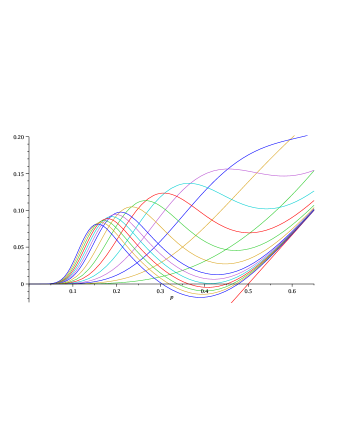
Figure 1. The relative correlation $\frac{\operatorname{\mathbb{P}{}}(a\mathrel{\not\to}s,s\mathrel{\not\to}b)-\operatorname{\mathbb{P}{}}(a\mathrel{\not\to}s)\operatorname{\mathbb{P}{}}(s\mathrel{\not\to}b)}{\operatorname{\mathbb{P}{}}(a\mathrel{\not\to}s,s\mathrel{\not\to}b)}$ in ${\vec{G}(n,p)}$ for $n=8,10,12,14,16,18,20,22,24,25,26,27,28,29,30$, and the asymptote $(2p-1)/3$. All curves are negative for very small $p$. For $n\geq 27$ we get three zeros.

For larger values of $n$ it becomes infeasible for our computers to obtain the exact functions. We have instead for various fixed values of $p$ used the recursions to obtain the value of the quotient $(g_{n}(p)-f_{n}(p)^{2})/g_{n}(p)$ for $n\leq 300$. Based on these calculations we conjecture the following.

Conjecture 6.1.

For $n\geq 27$, the relative covariance changes sign at three critical probabilities $p_{1}(n)<p_{2}(n)<p_{3}(n)$.

Conjecture 6.2.

Asymptotically, $p_{1}(n)\sim c_{1}/n$ and $p_{2}(n)\sim c_{2}/n$ for some constants $c_{1}$ and $c_{2}$.

The computations indicate that very rough estimates of $c_{1}$ and $c_{2}$ are $0.36$ and $7.5$, respectively.

It follows from Remark 4.6 that there is a critical probability $p(n)$ such that $p(n)\to 1/2$ exponentially fast; if our conjectures hold, this critical probability is thus $p_{3}(n)$.

Conjecture 6.3.

For all $n\geq 27$, $p_{3}(n)<1/2$.

Conjecture 6.4.

For $n\geq 8$, the relative covariance $\frac{\operatorname{\mathbb{P}{}}(a\mathrel{\not\to}s,s\mathrel{\not\to}b)-\operatorname{\mathbb{P}{}}(a\mathrel{\not\to}s)\operatorname{\mathbb{P}{}}(s\mathrel{\not\to}b)}{\operatorname{\mathbb{P}{}}(a\mathrel{\not\to}s,s\mathrel{\not\to}b)}>\frac{2p-1}{3}$.

Note that Conjecture 6.4 implies Conjecture 6.3 and the following related conjecture.

Conjecture 6.5.

For $p=\frac{1}{2}$, and $n\geq 6$ the relative covariance $\frac{\operatorname{\mathbb{P}{}}(a\mathrel{\not\to}s,s\mathrel{\not\to}b)-\operatorname{\mathbb{P}{}}(a\mathrel{\not\to}s)\operatorname{\mathbb{P}{}}(s\mathrel{\not\to}b)}{\operatorname{\mathbb{P}{}}(a\mathrel{\not\to}s,s\mathrel{\not\to}b)}$ is positive.

7. Exact recursions in ${\vec{G}(n,m)}$

For convenience, let $A:=\{a\mathrel{\not\to}s\}$ and $B:=\{s\mathrel{\not\to}b\}$. In this section we will derive recursions for $\operatorname{\mathbb{P}{}}(A)$ and $\operatorname{\mathbb{P}{}}(A\cap B)$ in ${\vec{G}(n,m)}$ using the corresponding exact recursions in ${\vec{G}(n,p)}$ from Section 5.

Let as above $f_{n}(p):=\operatorname{\mathbb{P}{}}_{{\vec{G}(n,p)}}(A)=\operatorname{\mathbb{P}{}}_{{\vec{G}(n,p)}}(B)$ and $g_{n}(p):=\operatorname{\mathbb{P}{}}_{{\vec{G}(n,p)}}(A\cap B)$, and let $h_{n}(m):=\operatorname{\mathbb{P}{}}_{{\vec{G}(n,m)}}(A)=\operatorname{\mathbb{P}{}}_{{\vec{G}(n,m)}}(B)$ and $k_{n}(m):=\operatorname{\mathbb{P}{}}_{{\vec{G}(n,m)}}(A\cap B)$. Further, let $N:=\binom{n}{2}$ be the number of edges in the complete graph $K_{n}$ and $M\sim\operatorname{Bin}(N,p)$ be the actual number of edges in $G(n,p)$. Using that $G(n,m)$ can be seen as $\bigl{(}G(n,p)\mid M=m\bigr{)}$, we can express the functions $f_{n}(p)$ and $g_{n}(p)$ for ${\vec{G}(n,p)}$ using the corresponding functions, $h_{n}(m)$ and $k_{n}(m)$, for ${\vec{G}(n,m)}$.

$$f_{n}(p) =\sum_{m=0}^{N}\operatorname{\mathbb{P}{}}(M=m)\cdot h_{n}(m)=\sum_{m=0}^{N}\binom{N}{m}p^{m}(1-p)^{N-m}\cdot h_{n}(m),$$

$$g_{n}(p) =\sum_{m=0}^{N}\operatorname{\mathbb{P}{}}(M=m)\cdot k_{n}(m)=\sum_{m=0}^{N}\binom{N}{m}p^{m}(1-p)^{N-m}\cdot k_{n}(m).$$

These relations can be inverted by repeated differentiating.

Theorem 7.1.

$$h_{n}(m) =\frac{(N-m)!}{N!}f_{n}^{(m)}(0)-\sum_{i=0}^{m-1}\binom{m}{i}(-1)^{m-i}\cdot h_{n}(i),$$

$$k_{n}(m) =\frac{(N-m)!}{N!}g_{n}^{(m)}(0)-\sum_{i=0}^{m-1}\binom{m}{i}(-1)^{m-i}\cdot k_{n}(i).$$

Proof.

It is sufficient to show one of the recursions.

$$f_{n}(p) =\sum_{i=0}^{N}\binom{N}{i}p^{i}(1-p)^{N-i}\cdot h_{n}(i)$$

$$=\sum_{i=0}^{N}\binom{N}{i}\sum_{j=0}^{N-i}\binom{N-i}{j}p^{i+j}(-1)^{j}\cdot h_{n}(i)$$

$$=\sum_{k=0}^{N}\frac{N!}{(N-k)!}p^{k}\sum_{i=0}^{k}\frac{1}{i!(k-i)!}(-1)^{k-i}\cdot h_{n}(i).$$

Differentiating $m$ times and inserting $p=0$ gives

$$f_{n}^{(m)}(0) =\frac{N!}{(N-m)!}m!\sum_{i=0}^{m}\frac{1}{i!(m-i)!}(-1)^{m-i}\cdot h_{n}(i)$$

from which we get

$$\sum_{i=0}^{m}\binom{m}{i}(-1)^{m-i}\cdot h_{n}(i)=\frac{(N-m)!}{N!}f_{n}^{(m)}(0),$$

which, after rearranging, gives the desired recursion. ∎

Computer calculations based on these recursions lead us to the following conjecture.

Conjecture 7.2.

For any fixed $n\geq 5$, the covariance in ${\vec{G}(n,m)}$ changes sign only once between two values of $m$.

8. Comparison between ${\vec{G}(n,p)}$ and ${\vec{G}(n,m)}$

As before, let $A:=\{a\mathrel{\not\to}s\}$ and $B:=\{s\mathrel{\not\to}b\}$. For moderate $n$, the correlation between $A$ and $B$ is positive in ${\vec{G}(n,p)}$ for quite small $p$, while, for ${\vec{G}(n,m)}$ the proportion of links, $m/N$, where $N=\binom{n}{2}$, needs to be closer to 1 to get a positive correlation. In fact, we may study the conditional covariance given $M\sim\operatorname{Bin}(N,p)$ to show that the covariance in ${\vec{G}(n,p)}$ exceeds the average covariance in ${\vec{G}(n,m)}$ for fixed $n$ and $p$.

Fact 8.1.

$$\operatorname{Cov}_{{\vec{G}(n,p)}}(A,B)=\operatorname{\mathbb{E}{}}(\operatorname{Cov}(A,B\mid M))+\operatorname{Var}(\operatorname{\mathbb{P}{}}(A\mid M))$$ (19)

where

$$\operatorname{\mathbb{E}{}}(\operatorname{Cov}(A,B\mid M))=\sum_{m=0}^{N}\operatorname{\mathbb{P}{}}(M=m)\cdot\operatorname{Cov}_{{\vec{G}(n,m)}}(A,B).$$

To understand this statement (a standard type of variance analysis) we will as in Section 7 view $G(n,m)$ as $(G(n,p)\mid M=m)$. Note that

$$\operatorname{Cov}_{{\vec{G}(n,p)}}(A,B) =\operatorname{\mathbb{P}{}}_{{\vec{G}(n,p)}}(A\cap B)-\operatorname{\mathbb{P}{}}_{\vec{G}(n,p)}(A)\operatorname{\mathbb{P}{}}_{\vec{G}(n,p)}(B)$$

$$=\operatorname{\mathbb{E}{}}(\operatorname{\mathbb{P}{}}(A\cap B\mid M))-\operatorname{\mathbb{E}{}}(\operatorname{\mathbb{P}{}}(A\mid M)\operatorname{\mathbb{P}{}}(B\mid M))$$

$$\hskip 40.00006pt+\operatorname{\mathbb{E}{}}(\operatorname{\mathbb{P}{}}(A\mid M)\operatorname{\mathbb{P}{}}(B\mid M))-\operatorname{\mathbb{E}{}}(\operatorname{\mathbb{P}{}}(A\mid M))\operatorname{\mathbb{E}{}}(\operatorname{\mathbb{P}{}}(B\mid M))$$

$$=\operatorname{\mathbb{E}{}}(\operatorname{Cov}(A,B\mid M))+\operatorname{Cov}(\operatorname{\mathbb{P}{}}(A\mid M),\operatorname{\mathbb{P}{}}(B\mid M))$$

and, as $\operatorname{\mathbb{P}{}}(A\mid M)=\operatorname{\mathbb{P}{}}(B\mid M)$, the formula follows.

The left-hand side of (19) is $\sim(2p-1)(1-p/2)^{2n-3}$ by Theorem 2.1. We can obtain the asymptotics of the two terms on the right-hand side too.

Theorem 8.2.

For every fixed $p\in(0,1]$,

$$\operatorname{\mathbb{E}{}}(\operatorname{Cov}(A,B\mid M)) =\Bigl{(}3-(4-2p)e^{2\frac{p(1-p)}{(2-p)^{2}}}+o(1)\Bigr{)}\bigl{(}1-p/2\bigr{)}^{2n-3},$$

$$\operatorname{Var}(\operatorname{\mathbb{P}{}}(A\mid M)) =4\Bigl{(}e^{2\frac{p(1-p)}{(2-p)^{2}}}-1+o(1)\Bigr{)}\bigl{(}1-p/2\bigr{)}^{2n-2}.$$

Note that all three terms in (19), as well as $\operatorname{\mathbb{P}{}}(A)\operatorname{\mathbb{P}{}}(B)=\operatorname{\mathbb{P}{}}(A)^{2}$, are of the same order (except when a term vanishes), viz.  $(1-p/2)^{2n}$, see Theorem 2.1 and Lemma 4.2.

Proof.

The sum of the right-hand sides equals $(2p-1+o(1))(1-p/2)^{2n-3}$, so by (1) and (19), it suffices to prove the second formula.

Let $\hat{p}=M/N=M/\binom{n}{2}$, and note that by the Law of Large Numbers, $\hat{p}\overset{\mathrm{p}}{\longrightarrow}p$. We begin by observing that by the Central Limit Theorem,

$$n(\hat{p}-p)=\frac{n}{N^{1/2}}\cdot\frac{M-Np}{N^{1/2}}\overset{\mathrm{d}}{\longrightarrow}\sqrt{2p(1-p)}Z,$$

where $\overset{\mathrm{d}}{\longrightarrow}$ denotes convergence in distribution and $Z\sim N(0,1)$ is a standard normal variable. It follows that for any real constants $a$ and $b$,

$$\frac{(1-\hat{p}/2)^{an+b}}{(1-p/2)^{an+b}}=\left(1-\frac{\hat{p}-p}{2-p}\right)^{an+b}\overset{\mathrm{d}}{\longrightarrow}\exp\left(a\frac{\sqrt{2p(1-p)}}{2-p}Z\right).$$ (20)

By Lemma 4.3,

$$\begin{split}\frac{\operatorname{\mathbb{P}{}}(A\mid M)}{(1-\hat{p}/2)^{n-1}}&=2e^{-\frac{\hat{p}(1-\hat{p})}{(2-\hat{p})^{2}}}+o_{\mathrm{p}}(1)=2e^{-\frac{p(1-p)}{(2-p)^{2}}}+o_{\mathrm{p}}(1),\end{split}$$

and thus by (20)

$$\frac{\operatorname{\mathbb{P}{}}(A\mid M)}{(1-p/2)^{n-1}}\overset{\mathrm{d}}{\longrightarrow}{2e^{-\frac{p(1-p)}{(2-p)^{2}}}}\exp\left(\frac{\sqrt{2p(1-p)}}{2-p}Z\right).$$ (21)

Denote the right-hand side of (21) by $R$. Since $\operatorname{\mathbb{E}{}}e^{cZ}=e^{c^{2}/2}$ for any real $c$, we have

$$\operatorname{\mathbb{E}{}}R^{r}=2^{r}e^{(r^{2}-r)\frac{p(1-p)}{(2-p)^{2}}},$$

in particular, $\operatorname{\mathbb{E}{}}R^{2}=4e^{2\frac{p(1-p)}{(2-p)^{2}}}$ and $\operatorname{\mathbb{E}{}}R=2$, so $\operatorname{Var}R=4e^{2\frac{p(1-p)}{(2-p)^{2}}}-4$. Hence the result follows if the variance converges in (21). For this, it suffices to show that

$$\operatorname{\mathbb{E}{}}\left(\frac{\operatorname{\mathbb{P}{}}(A\mid M)}{(1-p/2)^{n-1}}\right)^{4}=O(1).$$ (22)

(See e.g. [7, Theorems 5.4.2 and 5.4.9] for this standard argument, and note that the same argument shows that all moments converge in (21).)

To verify (22), let $p_{0}=p/2$. The proof of Lemma 4.3 shows that the estimates in Lemma 4.3 (with $p$ replaced by $\hat{p}$) hold uniformly for $\hat{p}\geq p_{0}$. Since $q(n-1;n,m)\leq q^{\prime}(n-1;n,\hat{p})=(1-\hat{p}/2)^{n-1}$ by Lemma 3.2, this yields $\operatorname{\mathbb{P}{}}(A\mid M)=O\bigl{(}(1-\hat{p}/2)^{n-1}\bigr{)}$, provided $\hat{p}\geq p_{0}$. For $\hat{p}<p_{0}$, we simply use $\operatorname{\mathbb{P}{}}(A\mid M)\leq 1$. Hence, for some constant $C$,

$$\operatorname{\mathbb{E}{}}\left(\frac{\operatorname{\mathbb{P}{}}(A\mid M)}{(1-p/2)^{n-1}}\right)^{4}\leq(1-p/2)^{-4(n-1)}\operatorname{\mathbb{P}{}}(\hat{p}<p_{0})+C\operatorname{\mathbb{E}{}}\left(\frac{1-\hat{p}/2}{1-p/2}\right)^{4(n-1)}.$$ (23)

The first term on the right-hand side is bounded since $\operatorname{\mathbb{P}{}}(\hat{p}<p_{0})=\operatorname{\mathbb{P}{}}(M<Np_{0})\leq e^{-Np/8}$ by the Chernoff bound [10, Theorem 2.1]. For the second term we have, letting $h=8/(n(2-p))$ and recalling that $M$ is a sum of $N$ independent copies of $I\sim\operatorname{Bin}(1,p)$,

$$\begin{split}\operatorname{\mathbb{E}{}}\left(\frac{1-\hat{p}/2}{1-p/2}\right)^{4(n-1)}&=\operatorname{\mathbb{E}{}}\left(1-\frac{\hat{p}-p}{2-p}\right)^{4(n-1)}\leq\operatorname{\mathbb{E}{}}\exp\left(-4(n-1)\frac{\hat{p}-p}{2-p}\right)\\ &=\operatorname{\mathbb{E}{}}\exp\bigl{(}-h(M-Np)\bigr{)}=\left(\operatorname{\mathbb{E}{}}\exp\bigl{(}-h(I-p)\bigr{)}\right)^{N}.\end{split}$$

Now $\operatorname{\mathbb{E}{}}e^{-h(I-p)}\leq e^{h^{2}/8}$, see [9, (4.16)] (a weaker estimate suffices), and thus the last expression is bounded by $e^{Nh^{2}/8}=O(1)$. This shows (22) and completes the proof. ∎

Numerical computations using the recursions of Sections 5 and 7 also suggest that all three quantities in (19), normalized by e.g. $(1-p/2)^{2n-3}$, converge quickly unless $p$ is very small, cf. Remark 4.6; see Figure 2 for the case $n=30$.

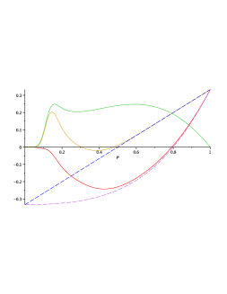
Figure 2. The solid curves are the covariance for $\vec{G}(30,p)$, middle curve, which by Fact 8.1 is the sum of the expected covariance for $\vec{G}(30,M)$, bottom, and $\operatorname{Var}(\operatorname{\mathbb{P}{}}(A\mid M))$, top curve. The dashed curves are the asymptotic curves for $\vec{G}(n,p)$ (straight line) and expected covariance for $\vec{G}(n,M)$. All curves normalized with $3(1-p/2)^{2n-3}$.

9. Quenched version

As mentioned in the introduction, we have so far studied the annealed model, i.e. the joint probability space of ${\vec{G}(n,p)}$ (or ${\vec{G}(n,m)}$) and that of the orientations. In the quenched model, the covariance is computed for each graph of ${\vec{G}(n,p)}$ (or ${\vec{G}(n,m)}$) and then averaged over all graphs.

It is quite common that the results differ between the two models, and this seems to be the case here also. We have computed the quenched expectations for ${\vec{G}(n,p)}$ (and ${\vec{G}(n,m)}$) for small $n$ ($n\leq 8$) and the covariances, as functions of $p$, look quite different, as can be seen from Figure 3 for $n=8$.

Figure 3. Annealed (top) and quenched (bottom) covariances for $\vec{G}(8,p)$.

For $n=4,\dots,8$ there is only one zero for the covariance, but this differs dramatically from the zero of the annealed model, as can be seen from Table 1.

$n$	Annealed	Quenched
4	1.000	1.000
5	0.729	0.927
6	0.276	0.857
7	0.152	0.809
8	0.107	0.783

Table 1. Zeroes of the covariances for ${\vec{G}(n,p)}$ in the annealed and quenched models.

Conditioning on the graph and taking expectations, we get that, similarly to Fact 8.1,

$$\operatorname{Cov}_{\vec{G}_{a}(n,p)}(A,B)=\operatorname{Cov}_{\vec{G}_{q}(n,p)}(A,B)+\operatorname{Cov}(\operatorname{\mathbb{P}{}}(A\mid G),\operatorname{\mathbb{P}{}}(B\mid G)),$$ (24)

where $\vec{G}_{a}(n,p)$ denotes the annealed model and $\vec{G}_{q}(n,p)$ denotes the quenched model; recall that $\operatorname{Cov}_{\vec{G}_{q}(n,p)}(A,B)$ is defined as $\operatorname{\mathbb{E}{}}_{\vec{G}_{q}(n,p)}(\operatorname{Cov}(A,B\mid G))$. (A similar formula holds for ${\vec{G}(n,m)}$ and the corresponding quenched model.)

Here the conditional probabilities for $A$ and $B$ given the graph need not be equal, so that the last covariance in (24) could possibly be negative for some values of $p$ and $n$. Even though our computations show that this is not the case when $n\leq 8$.

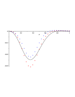
Figure 4. Covariances of $A$ and $B$ for $\vec{G}(8,p)$ (solid) and $\vec{G}(8,m)$ ($\circ$) in the quenched model and for $\vec{G}(8,m)$ ($+$) in the annealed model.

It is worth noting that, in contrast with the annealed model, in the quenched model ${\vec{G}(n,p)}$ and ${\vec{G}(n,m)}$ behave similarly, see Figure 4; this is not surprising, since the average taken in the quenched ${\vec{G}(n,p)}$ can be obtained by averaging over quenched ${\vec{G}(n,m)}$ with suitable weights. Also the quenched models appear, at least for small values of $n$, to be much closer to annealed ${\vec{G}(n,m)}$ than annealed ${\vec{G}(n,p)}$. In other words, the variation between different graphs with the same number of edges is of less importance than the variation caused by different number of edges. (The latter variation is quantified by Theorem 8.2.) This seems intuitively reasonable, since ${\vec{G}(n,m)}$ can be regarded as ${\vec{G}(n,p)}$ conditioned on the number of edges, which thus can be seen as a “semi-quenched” version.

Problem 9.1.

It would be interesting to find asymptotics for the quenched versions.

References

- [1] Sven Erick Alm & Svante Linusson, A counter-intuitive correlation in a random tournament, Preprint 2009, to appear in Combinatorics, Probability and Computing.
- [2] Sven Erick Alm & Svante Linusson, Correlations for paths in random orientations of , Preprint 2009 (earlier version of this paper), arXiv:0906.0720v1.
- [3] Jörgen Backelin, Multinomial expressions summation asymptotic approximations, Preprint 2010.
- [4] Jacob van den Berg, Olle Häggström & Jeff Kahn, Some conditional correlation inequalities for percolation and related processes, Random Structures and Algorithms 29 (2006), 417–435.
- [5] Jacob van den Berg & Jeff Kahn, A correlation inequality for connection events in percolation, Annals of Probability 29 (2001), no. 1, 123–126.
- [6] Geoffrey R. Grimmett, Infinite paths in randomly oriented lattices, Random Structures and Algorithms 18 (2001), no. 3, 257 – 266.
- [7] A. Gut, Probability: A Graduate Course. Springer, New York, 2005.
- [8] Olle Häggström, Probability on bunkbed graphs, Proceedings of FPSAC’03, Formal Power Series and Algebraic Combinatorics, Linköping, Sweden, 2003. Available at http://www.fpsac.org/FPSAC03/ARTICLES/42.pdf
- [9] W. Hoeffding, Probability inequalities for sums of bounded random variables, J. Amer. Statist. Assoc. 58 (1963) 13–30.
- [10] Svante Janson, Tomasz Łuczak & Andrzej Ruciński, Random Graphs, Wiley, New York, 2000.
- [11] Svante Linusson, On percolation and the bunkbed conjecture, Preprint 2008, to appear in Combinatorics, Probability and Computing.
- [12] Svante Linusson, A note on correlations in randomly oriented graphs, Preprint 2009, arXiv:0905.2881.
- [13] Colin McDiarmid, General percolation and random graphs, Adv. in Appl. Probab. 13 (1981), 40–60.