Discrete Dynamics: Gauge Invariance and Quantization

Abstract

Gauge invariance in discrete dynamical systems and its connection with quantization are considered. For a complete description of gauge symmetries of a system we construct explicitly a class of groups unifying in a natural way the space and internal symmetries. We describe the main features of the gauge principle relevant to the discrete and finite background. Assuming that continuous phenomena are approximations of more fundamental discrete processes, we discuss – with the help of a simple illustration – relations between such processes and their continuous approximations. We propose an approach to introduce quantum structures in discrete systems, based on finite gauge groups. In this approach quantization can be interpreted as introduction of gauge connection of a special kind. We illustrate our approach to quantization by a simple model and suggest generalization of this model. One of the main tools for our study is a program written in C.

1 Introduction

In 1918 Hermann Weyl – guided by the concept that the scale of length is arbitrary: if there is no fundamental length in Nature it does not matter what unit of length is used in measurements – conjectured that the scale can be taken in the form $e^{S({x})}$, i.e., it may vary from point to point in time and space. This idea failed in application to physics but gave rise to the concept of gauge invariance.

Later – in 1929, after advent of Quantum Mechanics – Weyl (and also Vladimir Fock and Fritz London) replaced scale transformations $e^{S({x})}$ by rotations (phase transformations) $e^{iS({x})}$ and derived electromagnetism from the gauge principle.

In 1954 C.N. Yang and R. Mills extended the gauge principle to non-Abelian symmetries. Now the gauge principle is recognized as one of the central principles in contemporary physics – in fact, all fundamental physical theories are gauge theories (for historical review see [1]).

The lattice gauge theory was introduced by K.G. Wilson in 1974 as a practical approach to the problems of strong interactions for which the standard perturbative methods are inapplicable. This technique – based on approximation of space, or space-time, by some (usually hypercubic) lattice – was considered as an auxiliary computational method rather than a fundamental construction. The later mathematical generalizations established relations between lattice gauge theories and such topics as topological quantum field theory (TQFT), invariants of 3- and 4-manifolds, monoidal categories, Hopf algebras and quantum groups, quantum gravity etc., [2].

In view of their origin and applications, the above mentioned lattice gauge theories are not entirely discrete constructions. They involve continuous ingredients: gauge groups are Lie groups, Lagrangians and observables are real or complex functions. Furthermore, the gauge groups of these theories are groups of internal symmetries and do not involve the lattice symmetries. It seems desirable to include the space symmetries into construction of gauge group, since: (a) the quantum statistics of particles is characterized by the rules describing their behavior under permutations of the points of space; (b) there exist gauge theories that deduce gravity by interpreting the space or space-time symmetries as gauge groups.

In this paper we consider more radical version of discrete gauge invariance. All our manipulations including quantization remain within the framework of exact discrete mathematics requiring no more than the ring of algebraic integers (and sometimes the quotient field of this ring). Our study was carried out with the help of a program in C we are developing now.

2 Discrete Dynamics

We consider evolution in the discrete time $t\in\mathbb{Z}=\left\{\ldots,-1,0,1,\ldots\right\}$.

Let the space $X$ be a finite set of points: $X=\left\{x_{1},\ldots,x_{N_{X}}\right\}$. This – primordially amorphous – set may possess some structure: some points may be “closer” to each other than others. A mathematical abstraction of such a structure is an abstract simplicial complex – a collection of subsets of $X$ (simplices) such that any subset of a simplex is also simplex. One-dimensional complexes, i.e., graphs (or lattices), are sufficient to formulate a gauge theory. The symmetry group of the space $X$ is the graph automorphism group $G=\mathrm{Aut}\left(X\right)$.

Table 1 shows some lattices with their symmetries. We use these lattices in our computer experiments. In the table $N_{X}$ and $N_{E}$ are numbers of points and vertices in space $X$; the trivial, symmetric, cyclic, dihedral and alternating groups are denoted by $1$, $\mathrm{Sym}\left(n\right)$, $\mathbb{Z}_{n}$, $\mathrm{D}_{2n}$ and $\mathrm{Alt}\!\left(n\right)$, respectively; the signs $\times$ and $\rtimes$ denote direct and semidirect products, respectively. Note, that the lattice denoted as Toric square $n\times{}n$ in the table has three times larger symmetry group at $n=4$ than the general case formula predicts.

Table 1: Examples of discrete spaces

$X$	$N_{X}$	$N_{E}$	$G$	$\left|G\right|$
Atom	$1$	$0$	$1$	$1$
Dimer	$2$	$1$	$\mathrm{Sym}\left(2\right)\cong\mathbb{Z}_{2}$	$2$
Triangle	$3$	$3$	$\mathrm{Sym}\left(3\right)\cong\mathrm{D}_{6}$	$6$
$n$-vertex polygon	$n$	$n$	$\mathrm{D}_{2n}$	$2n$
Tetrahedron	$4$	$6$	$\mathrm{Sym}\left(4\right)$	$24$
Octahedron	$6$	$12$	$\mathbb{Z}_{2}\times\mathrm{Sym}\left(4\right)$	$48$
Hexahedron	$8$	$12$	$\mathbb{Z}_{2}\times\mathrm{Sym}\left(4\right)$	$48$
Toric square $n{}\times{}n,n{}\neq{}4$	$n^{2}$	$2n^{2}$	$\left(\mathbb{Z}_{n}\times\mathbb{Z}_{n}\right)\rtimes\mathrm{D}_{8}$	$8n^{2}$
$n=4$	$16$	$32$	$\left(\left(\left(\left(\mathbb{Z}_{2}{}\times\mathrm{D}_{8}\right){}\rtimes\mathbb{Z}_{2}\right){}\rtimes{\color[rgb]{1,0,0}\mathbb{Z}_{3}}\right){}\rtimes\mathbb{Z}_{2}\right)\rtimes\mathbb{Z}_{2}$	$384$
Icosahedron	$12$	$30$	$\mathbb{Z}_{2}\times\mathrm{Alt}\!\left(5\right)$	$120$
Dodecahedron	$20$	$30$	$\mathbb{Z}_{2}\times\mathrm{Alt}\!\left(5\right)$	$120$
Fullerene $C_{60}$	$60$	$90$	$\mathbb{Z}_{2}\times\mathrm{Alt}\!\left(5\right)$	$120$
Toric graphene $n\times m$	$nm$	${}\frac{\textstyle{3nm}}{\textstyle{2}}{}$	$\mathrm{D}_{n}\times\mathrm{D}_{2m}$	$2nm{}$

Let each point $x\in X$ take values in some finite set of local states $\Sigma=\left\{\sigma_{1},\ldots,\sigma_{N_{\Sigma}}\right\}$ possessing some symmetry group $\Gamma\leq\mathrm{Sym}\left(\Sigma\right).$ Such groups are analogs of the “groups of internal symmetries” responsible for interactions in physical gauge theories. The state of a system as a whole is a function $\sigma(x)\in\Sigma^{X}.$

Dynamics of the system is determined by some evolution rule connecting the current state of the system $\sigma_{t}(x)$ with its prehistory $\sigma_{t-1}(x),~{}\sigma_{t-2}(x),\ldots\enspace.$
A typical form of evolution rule is evolution relation:

$$R\left(\sigma_{t}\left(x\right);~{}\sigma_{t-1}\left(x\right),~{}\sigma_{t-2}\left(x\right),\ldots\right)\subseteq\Sigma^{X}\times\Sigma^{X}\times\cdots\enspace.$$ (1)

Most commonly used in applications and convenient for study are deterministic (or causal) dynamical systems. The current state of deterministic system is uniquely determined by its prehistory, i.e., relations like (1) are functional and can be written in the form

$$\sigma_{t}\left(x\right)=F\left(\sigma_{t-1}\left(x\right),\sigma_{t-2}\left(x\right),\ldots\right)\enspace.$$

There are two important special types of non-deterministic dynamical systems:

• lattice models in statistical mechanics – special instances of Markov chains;

• discrete quantum systems obtained from classical systems by identification of their states with basis elements of complex Hilbert spaces.

For these systems transition from one state to any other is possible with some probability controlled by additional structures: real (for Markov chains) or complex (for quantum systems) weights assigned to state transitions. In this paper we restrict our attention to the case of discrete quantum systems.

3 Unification of Space and Internal Symmetries

Having the groups $G$ and $\Gamma$ acting on $X$ and $\Sigma$, respectively, we can combine them into a single group ${W}$ which acts on the states $\Sigma^{X}$ of the whole system. The group ${W}$ can be identified, as a set, with the Cartesian product $\Gamma^{X}\otimes G$, where $\Gamma^{X}$ is the set of $\Gamma$-valued functions on $X.$ That is, every element $u\in{W}$ can be represented in the form $u=\left({\alpha(x)},~{}{a}\right),$ where $\alpha(x)\in\Gamma^{X}$ and $a\in G.$

In physics, it is usually assumed that the space and internal symmetries are independent, i.e., ${W}$ is the direct product $\Gamma^{X}\times G$ with action on $\Sigma^{X}$ and multiplication rule:

$$\sigma(x)\left({\alpha\left(x\right)},~{}{a}\right) = \sigma\left(x\right)\alpha\left(x\right)\text{~{}~{}~{}~{}~{}~{}~{}~{}~{}~{}~{}\emph{action}}\enspace,$$

$$\left({\alpha\left(x\right)},~{}{a}\right)\ast\left({\beta\left(x\right)},~{}{b}\right) = \left({\alpha\left(x\right)\beta\left(x\right)},~{}{ab}\right)\text{~{}~{}~{}~{}\emph{multiplication}}\enspace.$$ (2)

Another standard construction is the wreath product $\Gamma\wr_{X}G$ having a structure of the semidirect product $\Gamma^{X}\rtimes G$ with action and multiplication

$$\sigma(x)\left({\alpha\left(x\right)},~{}{a}\right) = \sigma\left(xa^{-1}\right)\alpha\left(xa^{-1}\right)\enspace,$$

$$\left({\alpha\left(x\right)},~{}{a}\right)\ast\left({\beta\left(x\right)},~{}{b}\right) = \left({\alpha\left(x\right)\beta\left(xa\right)},~{}{ab}\right)\enspace.$$ (3)

These examples are generalized by the following Statement:
There are equivalence classes of split group extensions $1\rightarrow\Gamma^{X}\rightarrow{W}\rightarrow G\rightarrow 1$ determined by antihomomorphisms $\mu:G\rightarrow G$. The equivalence is described by arbitrary function $\kappa:G\rightarrow G.$ The explicit formulas for main group operations — action on $\Sigma^{X}$, multiplication and inversion — are

$$\sigma(x)\left({\alpha\left(x\right)},~{}{a}\right) = \sigma\left(x\mu(a)\right)\alpha\left(x\kappa(a)\right)\enspace,$$ (4)

$$\left({\alpha\left(x\right)},~{}{a}\right)\ast\left({\beta\left(x\right)},~{}{b}\right) = \left({\alpha\left(x\kappa(ab)^{-1}\mu(b)\kappa(a)\right)\beta\left(x\kappa(ab)^{-1}\kappa(b)\right)},~{}{ab}\right)\enspace,$$ (5)

$$\left({\alpha(x)},~{}{a}\right)^{-1} = \left({\alpha\left(x\kappa\left(a^{-1}\right)^{-1}\mu(a)^{-1}\kappa(a)\right)^{-1}},~{}{a^{-1}}\right)\enspace.$$ (6)

This statement follows from the general description of the structure of split extensions of a group $G_{1}$ by a group $G_{0}$: all such extensions are determined by the homomorphisms from $G_{1}$ to $\mathrm{Aut}\left(G_{0}\right)$ (see, e.g., [3], p. 18). Specializing this description to the case when $G_{0}$ is the set of $\Gamma$-valued function on $X$ and $G_{1}$ acts on arguments of these functions we obtain our statement. The equivalence of extensions with the same antihomomorfism $\mu$ but with different functions $\kappa$ is expressed by the commutative diagram

$$\begin{diagram}\enspace,$$ (7)

where the mapping $K$ takes the form $K:\left({\alpha(x)},~{}{a}\right)\mapsto\left({\alpha\left(x\kappa(a)\right)},~{}{a}\right)\enspace.$

Note that the standard direct (2) and wreath (3) products are obtained from this general construction by choosing $\left(\mu(a)=1,\kappa(a)=1\right)$ and $\left(\mu(a)=a^{-1},\right.$ $\left.\kappa(a)=a^{-1}\right)$, respectively.

In our C program the group ${W}$ is specified by two groups $G$ and $\Gamma$ and two functions $\mu(a)$ and $\kappa(a)$ implemented as arrays. It is convenient in computations to use the following specialization: $\mu(a)=a^{-m}$ and $\kappa(a)=a^{k}$. For such a choice formulas (4-6) take the form

$$\sigma(x)\left({\alpha\left(x\right)},~{}{a}\right) = \sigma\left(xa^{-m}\right)\alpha\left(xa^{k}\right)\enspace,$$ (8)

$$\left({\alpha\left(x\right)},~{}{a}\right)\ast\left({\beta\left(x\right)},~{}{b}\right) = \left({\alpha\left(x(ab)^{-k-m}a^{k+m}\right)\beta\left(x(ab)^{-k}b^{k}\right)},~{}{ab}\right)\enspace,$$ (9)

$$\left({\alpha(x)},~{}{a}\right)^{-1} = \left({\alpha\left(xa^{2k+m}\right)^{-1}},~{}{a^{-1}}\right)\enspace.$$ (10)

Here $k$ is arbitrary integer, $m=0$ (direct product) or $m=1$ (wreath product).

4 Discrete Gauge Principle

In fact, the gauge principle expresses the very general idea that any observable data can be presented in different “frames” at different points of space and time, and there should be some way to compare these data. At the set-theoretic level, i.e., in the form suitable for both discrete and continuous cases, the main concepts of the gauge principle can be reduced to the following elements

• a set $X$, space or space-time;

• a set $\Sigma$, local states;

• the set $\Sigma^{X}$ of $\Sigma$-valued functions on $X$, the set of states of dynamical system;

• a group ${W}\leq\mathrm{Sym}\left(\Sigma^{X}\right)$ acting on $\Sigma^{X}$, symmetries of the system;

• identification of data describing dynamical system with states from $\Sigma^{X}$ makes sense only modulo symmetries from ${W}$;

• having no a priori connection between data from $\Sigma^{X}$ at different points $x$ and $y$ in time and space we impose this connection (or parallel transport) explicitly as ${W}$-valued functions on edges of abstract graph:

  $$P(x,y)\in{W},~{}\varsigma(y)=\sigma(x)P(x,y)\enspace;$$

  connection $P(x,y)$ has obvious property $P(y,x)=P(x,y)^{-1};$

• connection $P(x,y)$ is called trivial if it can be expressed in terms of a function on vertices of the graph: $P(x,y)=p(x)^{-1}p(y),~{}p(x),p(y)\in{W};$

• invariance with respect to gauge symmetries depending on time or space $u(x),u(y)\in{W}$ leads to transformation rule for connection

  $$P(x,y)\rightarrow u(x)^{-1}P(x,y)u(y);$$ (11)

• the curvature of connection $P(x,y)$ is defined as the conjugacy class of the holonomy along a cycle of a graph:

  $$P(x_{1},x_{2},\ldots,x_{k})=P(x_{1},x_{2})P(x_{2},x_{3})\cdots P(x_{k},x_{1})$$

  (the conjugacy means $P^{\prime}(x_{1},\ldots,x_{k})\sim u^{-1}P(x_{1},\ldots,x_{k})u$ for any $u\in{W}$);
  the curvature of trivial connection is obviously trivial: $\widetilde{P}(x_{1},\ldots,x_{k})\equiv 1;$

• the gauge principle does not tell us anything about the evolution of the connection itself, so gauge invariant relation describing dynamics of connection (gauge field) should be added.

Let us give two illustrations of how these concepts work in continuous case.

Electrodynamics. Abelian prototype of all gauge theories.

Here the set $X$ is 4-dimensional Minkowski space with points $x=\left(x^{\mu}\right)$ and the set of states is Hilbert space of complex scalar (Schrödinger equation) or spinor (Dirac equation) fields $\psi(x).$ The symmetry group of the Lagrangians and physical observables is ${W}=\mathrm{U}(1).$ The elements of $\mathrm{U}(1)$ can be represented as $e^{-i\alpha}.$

Let us make these elements dependent on space-time and consider the parallel transport for two closely situated space-time points:

$$P(x,x+\Delta x)=e^{-i\rho(x,x+\Delta x)}\enspace.$$

Specializing transformation rule (11) to this particular case

$$P^{\prime}(x,x+\Delta x)=e^{i\alpha(x)}P(x,x+\Delta x)e^{-i\alpha(x+\Delta x)}\enspace,$$

substituting approximations

$$P(x,x+\Delta x)=e^{-i\rho(x,x+\Delta x)}\approx 1-i{A}(x)\Delta x\enspace,$$

$$P^{\prime}(x,x+\Delta x)=e^{-i\rho(x,x+\Delta x)}\approx 1-i{A^{\prime}}(x)\Delta x\enspace,$$

$$e^{-i\alpha(x+\Delta x)}\approx e^{-i\alpha(x)}\left(1-i\nabla\alpha(x)\Delta x\right)\enspace,$$

and taking into account commutativity of ${W}=\mathrm{U}(1)$ we obtain

$${A^{\prime}}(x)={A}(x)+\nabla\alpha(x)\enspace~{}~{}\mbox{or, in components,}\enspace~{}~{}{A^{\prime}_{\mu}}(x)={A_{\mu}}(x)+\frac{\textstyle{\partial\alpha(x)}}{\textstyle{\partial x^{\mu}}}\enspace.$$ (12)

The 1-form $A$ taking values in the Lie algebra of $\mathrm{U}(1)$ and its differential $F=\left(F_{\mu\nu}\right)=\mathrm{d}A$ are identified with the electromagnetic vector potential and field strength, respectively. To provide the gauge invariance of the equations for field $\psi(x)$ we should replace partial by covariant derivatives

$$\partial_{\mu}\rightarrow D_{\mu}=\partial_{\mu}-iA_{\mu}(x)$$

in those equations.

Finally, evolution equations for the gauge field $A(x)$ should be added. In the case of electromagnetics these are Maxwell’s equations:

$$\mathrm{d}F = 0\hskip 20.0pt\text{\emph{first pair}}$$ (13)

$$\mathrm{d}\star F = 0\hskip 20.0pt\text{\emph{second pair}}.$$ (14)

Here $\star$ is the Hodge conjugation (Hodge star operator). Note that equation (14) corresponds to vacuum Maxwell’s equations. In the presence of the current $J~{}$ the second pair takes the form $~{}~{}\star\mathrm{d}\star F=J.$ Note also that the first pair is essentially a priori statement, it reflects simply the fact that $F$, by definition, is the differential of an exterior form.

Non-Abelian gauge theories in continuous space-time.

Only minor modifications are needed for the case of non-Abelian Lie group ${W}.$ Again expansion of the ${W}$-valued parallel transport for two close space-time points $x$ and $x+\Delta x$ with taking into account that $P(x,x)=1$ leads to introducing of a Lie algebra valued 1-form $A=\left(A_{\mu}\right):$

$$P(x,x+\Delta x)\approx 1+A_{\mu}(x)\Delta x^{\mu}\enspace.$$

Infinitesimal manipulations with formula (11)

$$u(x)^{-1}P(x,x+\Delta x)u(x+\Delta x)~{}\longrightarrow~{}u(x)^{-1}\left(1+A_{\mu}(x)\Delta x^{\mu}\right)\left(u(x)+\frac{\textstyle{\partial u(x)}}{\textstyle{\partial x^{\mu}}}\Delta x^{\mu}\right)$$

lead to the following transformation rule

$${A^{\prime}_{\mu}}(x)=u(x)^{-1}{A_{\mu}}(x)u(x)+u(x)^{-1}\frac{\textstyle{\partial u(x)}}{\textstyle{\partial x^{\mu}}}\enspace.$$ (15)

The curvature 2-form

$$F=dA+\left[A\wedge A\right]$$

is interpreted as physical strength field. In particular, the trivial connection

$$\widetilde{A}_{\mu}(x)=u_{0}(x)^{-1}\frac{\textstyle{\partial u_{0}(x)}}{\textstyle{\partial x^{\mu}}}$$

is flat, i.e., its curvature $F=0.$

There are different approaches to construct dynamical equations for gauge fields [2]. The most important example is Yang-Mills theory based on the Lagrangian

$$L_{YM}=\mathrm{Tr}\left[F\wedge\star F\right]\enspace.$$

The Yang-Mills equations of motion read

$$\mathrm{d}F+\left[A\wedge F\right] = 0\enspace,$$ (16)

$$\mathrm{d}\star F+\left[A\wedge\star F\right] = 0\enspace.$$ (17)

Here again equation (16) is a priori statement called Bianci identity. Note that Maxwell’s equations are a special case of Yang-Mills equations.

It is instructive to see what the Yang-Mills Lagrangian looks like in the discrete approximation. Replacing the Minkowski space $X$ by a hypercubic lattice one can see that the discrete version of $L_{YM}$ is proportional to $\sum_{f}\sigma\left(\gamma_{f}\right)$, where the summation is over all faces of a hypercubic constituent of the lattice;

$$\sigma=2\dim{}U-\left(\chi_{U}+\chi_{U^{\dagger}}\right);$$

$\chi_{U}$ and $\chi_{U^{\dagger}}$ are characters of the fundamental representation $U$ of the gauge group and its dual representation, respectively; $\gamma_{f}$ is the gauge group holonomy around the face $f$.

The Yang-Mills theory uses Hodge operation converting $k$-forms to $(n-k)$-forms in $n$-dimensional space with metric $g_{\mu\nu}$. In topological applications so-called BF theory plays an important role since it does not involve a metric. In this theory, an additional dynamical field $B$ is introduced. The Lie algebra valued $(n-2)$-form $B$ and the $2$-form $F$ are combined into the Lagrangian $L_{BF}=\mathrm{Tr}\left[B\wedge F\right]\enspace.$

5 Quantization Based on Finite Group

Quantization is a procedure for recovering a more fundamental quantum theory from its classical approximation. Both Lagrangian and Hamiltonian formulations of classical mechanics are based on the principle of least action which looks a bit mysterious: a particle moving from one point to another “knows” in advance where it is going to arrive. Feynman’s path integral quantization [4] eliminates this apparent teleology in a quite natural way: classical trajectories correspond to the dominating (in the path integral) part of all possible trajectories.

Of course, recovering a theory from its approximation can not be performed uniquely. Moreover, discrepancies between a theory and its approximation may be essential. To illustrate, let us compare a simple discrete process with its approximation by continuous physical law.

5.1 Heat Equation from Bernoulli Trials

Let us consider a sequence of Bernoulli trials. The probability of a separate sequence is described by the binomial distribution

$$P\left(n_{-},n_{+}\right)=\frac{\left(n_{-}+n_{+}\right)!}{n_{-}!n_{+}!}p_{-}^{n_{-}}p_{+}^{n_{+}}\enspace.$$ (18)

Here $\left\{-,~{}+\right\}$ are possible outcomes of a single trial; $p_{-},~{}p_{+}$ are probabilities ($p_{-}+p_{+}=1$) and $n_{-},~{}n_{+}$ are numbers of the outcomes.

Applying  Stirling’s approximation  to (18) and introducing new variables $x=n_{+}-n_{-},~{}t=n_{-}+n_{+},~{}v=p_{-}-p_{+}$ — let us call them “space”, “time” and “velocity”, respectively — we obtain

$$P\left(x,t\right)\approx\widetilde{P}\left(x,t\right)=\frac{1}{\sqrt{1-v^{2}}}\sqrt{\frac{2}{\pi{}t}}\exp\left\{-\frac{1}{2t}\left(\frac{x-vt}{\sqrt{1-v^{2}}}\right)^{2}\right\}\enspace.$$ (19)

This is the fundamental solution of the heat (also known as diffusion or Fokker–Planck) equation:

$$\frac{\partial\widetilde{P}\left(x,t\right)}{\partial t}+v\frac{\partial\widetilde{P}\left(x,t\right)}{\partial x}=\frac{\left(1-v^{2}\right)}{2}\frac{\partial^{2}\widetilde{P}\left(x,t\right)}{\partial x^{2}}\enspace.$$ (20)

Note that expression (19) contains “relativistic” fragment $\frac{\textstyle{x-vt}}{\textstyle{\sqrt{1-v^{2}}}}$ due to the velocity limits $-1\leq v\leq 1$ in our model. Note also that at $\left|v\right|=1$ equation (20) reduces to the wave equation

$$\frac{\partial\widetilde{P}\left(x,t\right)}{\partial t}\pm\frac{\partial\widetilde{P}\left(x,t\right)}{\partial x}=0\enspace.$$ (21)

Now let us set a problem as is typical in mechanics: find extremal trajectories connecting two fixed points $(0,0)$ and $(X,T)$. We adopt here the search of trajectories with maximum probability as a version of the “least action principle”. The probability of trajectory passing through some intermediate point $(x,t)$ is the following conditional probability

$$P_{(0,0)\rightarrow(x,t)\rightarrow(X,T)} = \frac{P(x,t)P(X-x,T-t)}{P(X,T)}$$ (22)

$$= \frac{t!(T-t)!\left(\frac{T-X}{2}\right)!\left(\frac{T+X}{2}\right)!}{\left(\frac{t-x}{2}\right)!\left(\frac{t+x}{2}\right)!\left(\frac{T-t}{2}-\frac{X-x}{2}\right)!\left(\frac{T-t}{2}+\frac{X-x}{2}\right)!T!}\enspace.$$

The conditional probability computed for approximation (19) takes the form

$$\widetilde{P}_{(0,0)\rightarrow(x,t)\rightarrow(X,T)}=\frac{T}{\sqrt{\frac{\pi}{2}(1-v^{2})tT(T-t)}}\exp\left\{-\frac{\left(Xt-xT\right)^{2}}{2(1-v^{2})tT(T-t)}\right\}.$$ (23)

One can see essential differences between (22) and (23):

• exact probabilities (22) do not depend on the velocity $v$ (or on the probabilities $p_{-},~{}p_{+}$ of a single trial), whereas (23) contains artificial dependence,

• it is easy to check that expression (22) allows many trajectories with the same maximum probability, whereas extremals of (23) are deterministic trajectories, namely, straight lines  $x=\frac{X}{T}t.$

These artifacts show that an important guiding principle of quantization — correspondence with classical limit — may not be quite reliable.

5.2 Gauge Connection and Quantization

The Aharonov–Bohm effect (Fig. 1) is one of the most striking illustrations of interplay between quantum behavior and gauge connection. Charged particles moving through the region containing perfectly shielded thin solenoid produce different interference patterns on a screen depending on whether the solenoid is turned on or off. There is no electromagnetic force acting on the particles, but working solenoid produces $\mathrm{U}(1)$-connection adding or subtracting phases of the particles and, thus, changing the interference pattern.

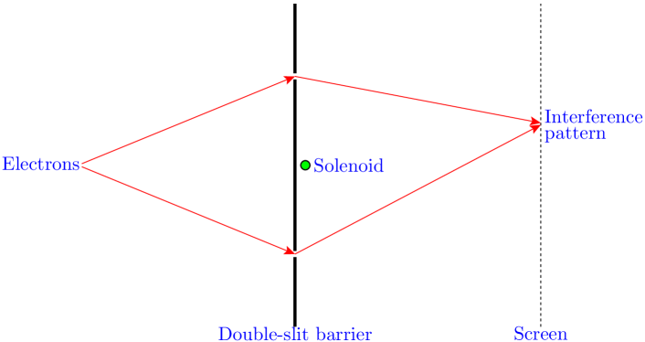
Figure 1: Aharonov–Bohm effect. Magnetic flux is confined within the perfectly shielded solenoid; interference pattern is shifted in spite of absence of electromagnetic forces acting on the particles.

In the discrete time Feynman’s path amplitude decomposes into the product of elements of the group $\mathrm{U}(1)$ (or, more precisely, elements of the fundamental representation of $\mathrm{U}(1)$):

$$A_{\mathrm{U}(1)}=\exp\left(iS\right)=\exp\left(i\int Ldt\right)\longrightarrow\mathrm{e}^{\textstyle{iL_{0,1}}}\ldots\mathrm{e}^{\textstyle{iL_{t-1,t}}}\ldots\mathrm{e}^{\textstyle{iL_{T-1,T}}}\enspace.$$ (24)

By the notation $L_{t-1,t}$ we emphasize that the Lagrangian is in fact a function defined on pairs of points (graph edges) — this is compatible with physics where the typical Lagrangians are determined by the first order derivatives. Thus, the expression $P(t-1,t)=e^{\textstyle{iL_{t-1,t}}}\in\mathrm{U}(1)$ can be interpreted as $\mathrm{U}(1)$-parallel transport. A natural generalization of this is to suppose that:

• the group $\mathrm{U}(1)$ can be replaced by some other group $\Gamma$,

• unitary representation $\rho\left(\Gamma\right)$ may have dimensionality different from 1.

We can introduce quantum mechanical description of a discrete system interpreting states $\sigma\in\Sigma$ as basis elements of a Hilbert space $\Psi$. This allows to describe statistics of observations of $\sigma^{,}s$ in terms of the inner product in $\Psi$.

Now let us replace expression (24) for Feynman’s path amplitude by the following parallel transport along the path

$$A_{\rho\left(\Gamma\right)}=\rho\left(\alpha_{0,1}\right)\ldots\rho\left(\alpha_{t-1,t}\right)\ldots\rho\left(\alpha_{T-1,T}\right)\enspace.$$

Here $\alpha_{t-1,t}$ are elements of a finite group $\Gamma$ – we shall call $\Gamma$ quantizing group – and $\rho$ is an unitary representation of $\Gamma$ on the space $\Psi$.

Let us recall main properties of linear representations of finite groups [5].

• First of all, any linear representation of finite group is equivalent to unitary.

• Any unitary representation $\rho$ is determined uniquely (up to isomorphism) by its character defined as $~{}~{}\chi_{\rho}(\alpha)=\mathrm{Tr}\rho(\alpha),~{}\alpha\in\Gamma.$

• All values of $\chi_{\rho}$ and eigenvalues of $\rho$ are elements of the ring $\mathbb{A}$ of algebraic integers, moreover the eigenvalues are roots of unity. Recall that the ring $\mathbb{A}$ consists of the roots of monic polynomials with integer coefficients [3].

• If all different irreducible representations of $\Gamma$ are $\rho_{1},\cdots,\rho_{i},\cdots,\rho_{h}$ and $d_{i}=\dim\rho_{i}$, $M=\left|\Gamma\right|$ then

  $${\sum\limits_{i-1}^{h}{}d_{i}^{2}=M}\text{~{}~{}and any~{}~{}}{d_{i}}\text{~{}~{}divides~{}~{}}{M}:~{}~{}{d_{i}\mid{}M}.$$

• Any function $\varphi(\alpha)$ depending only on conjugacy classes of $\Gamma$, i.e.,
  $\varphi\left(\beta^{-1}\alpha\beta\right)=\varphi\left(\alpha\right)$, is linear combination of characters $\chi_{\rho_{1}},\cdots,\chi_{\rho_{h}}$.
  Such functions are called central or class functions.

If the group $\Gamma$ consists of $M$ elements $\gamma_{0},\ldots,\gamma_{M-1}$ and $n_{k}$ is the number of paths with the “phase” $\Phi=\rho\left(\gamma_{k}\right)$ at the point of observation $\left(x,t\right)$, then the amplitude at this point is $A=\sum\limits_{k=0}^{M-1}n_{k}\rho\left(\gamma_{k}\right)\psi$, where $\psi\in\Psi$. The square of the amplitude (i.e., probability after appropriate normalization) can be written as

$$\left\langle A\psi|A\psi\right\rangle=\sum\limits_{{k=0}}^{{M-1}}n_{k}^{2}\left|\psi\right|^{2}+\sum_{\begin{subarray}{c}{\gamma_{i},\gamma_{k}\in\Gamma}\\ {i<k}\end{subarray}}n_{i}n_{k}\left\langle\psi\left|\rho\left(\gamma_{i}^{-1}\gamma_{k}\right)+\rho^{\dagger}\left(\gamma_{i}^{-1}\gamma_{k}\right)\right|\psi\right\rangle\enspace,$$ (25)

or, after collecting like terms, as

$$\left\langle A\psi|A\psi\right\rangle==\sum\limits_{k=0}^{M-1}N_{k}\left(n_{0},\cdots,n_{M-1}\right)\left\langle\psi\left|\rho\left(\gamma_{k}\right)+\rho^{\dagger}\left(\gamma_{k}\right)\right|\psi\right\rangle\enspace,$$ (26)

where $N_{k}\left(n_{0},\cdots,n_{M-1}\right)$ are quadratic polynomials with integer coefficients and arguments. Thus, algebraic integers are sufficient for all our computations except for normalization of probabilities requiring the quotient field of the ring $\mathbb{A}$.

5.3 Simple Model Inspired by Free Particle

In quantum mechanics – as is clear from the never vanishing expression $\exp\left(\frac{i}{\hbar}S\right)$ for the path amplitude – transitions from one to any other state are possible in principle. However, we shall consider computationally more tractable models with restricted sets of possible transitions.

Let us consider quantization of a free particle moving in one dimension. Such a particle is described by the Lagrangian $L=\frac{\textstyle{m\dot{x}^{2}}}{\textstyle{2}}.$ Keeping only transitions to the closest points in the discretized space we come to the following rule for the one-time-step transition amplitudes

$e^{\textstyle{\frac{i}{\hbar}\frac{m\left\{(x+1)-x\right\}^{2}}{2}}}=e^{\textstyle{i\frac{m}{2\hbar}}}$ $e^{\textstyle{\frac{i}{\hbar}\frac{m\left(x-x\right)^{2}}{2}}}\hskip 17.0pt=~{}1$ $e^{\textstyle{\frac{i}{\hbar}\frac{m\left\{(x-1)-x\right\}^{2}}{2}}}=e^{\textstyle{i\frac{m}{2\hbar}}}.$

That is, we have evolution rule as an $\mathrm{U}(1)$-valued function $R$ defined on pairs of points (graph edges). Symbolically:

$$R\left(x\rightarrow{}x\right) = 1~{}~{}\in~{}~{}\mathrm{U}(1)\enspace,$$

$$R\left(x\rightarrow{}x-1\right)=R\left(x\rightarrow{}x+1\right) = w=e^{\textstyle{i\frac{m}{2\hbar}}}~{}~{}\in~{}~{}\mathrm{U}(1)\enspace.$$ (27)

Now let us assume that $w$ in (27) is an element of some representation of a finite group: $w=\rho\left(\alpha\right),~{}\alpha\in\Gamma=\left\{\gamma_{0}=1,\ldots,\gamma_{M-1}\right\}$. Rearranging multinomial coefficients — trinomial in this concrete case — it is not difficult to write the sum amplitude over all paths of the form $\left(0,0\right)\longrightarrow\left(x,t\right)$

$$A_{x}^{t}\left(w\right)=\sum\limits_{\tau=0}^{t}\frac{\tau!}{\left(\frac{\tau-x}{2}\right)!\left(\frac{\tau+x}{2}\right)!}\times\frac{t!}{\tau!\left(t-\tau\right)!}~{}w^{\tau}\enspace.$$ (28)

Note that $x$ must lie in the limits determined by $t$: $x\in\left[-t,t\right].$

One of the most expressive peculiarities of quantum-mechanical behavior is the destructive interference — cancellation of non-zero amplitudes attached to different paths converging to the same point. By construction, the sum of amplitudes in our model is a function $A(w)$ depending on distribution of sources of the particles, their initial phases, gauge fields acting along the paths, restrictions – like, e.g., “slits” – imposed on possible paths, etc. In the case of one-dimensional representation the function $A(w)$ is a polynomial with algebraic integer coefficients and $w$ is a root of unity. Thus, the condition for destructive interference can be expressed by the system of polynomial equations: $A(w)=0$ and $w^{M}=1$. For concreteness let us consider the cyclic group $\Gamma=\mathbb{Z}_{M}=\left\{\gamma_{0},\cdots,\gamma_{k},\cdots,\gamma_{M-1}\right\}$. Any of its $M$ irreducible representations takes the form $\rho\left(\gamma_{k}\right)=w^{k}$, where $w$ is one of the $M$th roots of unity. For simplicity let $w$ be the primitive root: $w=\mathrm{e}^{2\pi{}i/M}.$ Fig. 2 shows all possible transitions from the point $x$ in three time steps with their amplitudes.

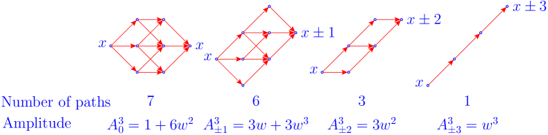
Figure 2: Amplitudes for all possible paths in three time steps.

We see that the polynomial $A^{3}_{\pm 1}=3w+3w^{3}=3w\left(w^{2}+1\right)$ contains the cyclotomic polynomial $\Phi_{4}(w)=w^{2}+1$ as a factor. The smallest group associated to $\Phi_{4}(w)$ — and hence providing the destructive interference — is $\mathbb{Z}_{4}$. Thus, $\mathbb{Z}_{4}$ is the natural quantizing group for the model under consideration.

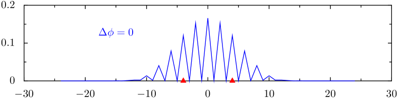
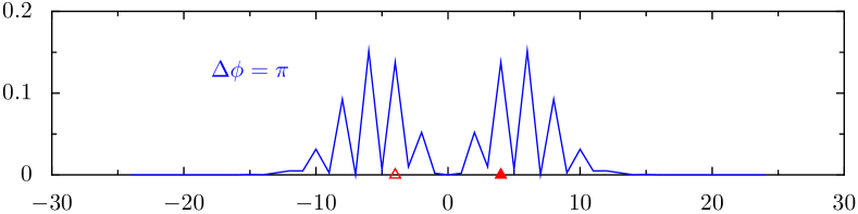
Figure 3: Group $\mathbb{Z}_{4}$. Interference from two sources. Number of time steps $T=20$. Source positions are -4 and 4. Phase differences $\Delta\phi=\phi_{4}-\phi_{-4}$ between sources are $0$ and $\pi$.

Fig. 3 shows interference patterns — normalized squared amplitudes (“probabilities”) — from two sources placed in the positions $x=-4$ and $x=4$ for 20 time steps. The upper and lower graphs show interference pattern when sources are in the same ($\Delta\phi=0$) and in the opposite ($\Delta\phi=\pi$) phases, respectively.

5.4 Generalization: Local Quantum Model on Regular Graph

The above model — with quantum transitions allowed only within the neighborhood of a vertex of a 1-dimensional lattice — can easily be generalized to arbitrary regular graph. Our definition of local quantum model on $k$-valent graph uncludes the following:

1. Space $X=\left\{x_{1},\cdots,x_{N}\right\}$ is a $k-$valent graph.

2. Set of local transitions $E_{i}=\left\{e_{0,i},e_{1,i},\cdots,e_{k,i}\right\}$ is the set of $k$ adjacent to the vertex $x_{i}$ edges $e_{m,i}=\left(x_{i}\rightarrow{}x_{m,i}\right)$ completed by the edge $e_{0,i}=\left(x_{i}\rightarrow{}x_{i}\right)$.

3. We assume that the space symmetry group $G=\mathrm{Aut}\left(X\right)$ acts transitively on the set $\left\{E_{1},\cdots,E_{N}\right\}$.

4. $G_{i}=\mathrm{Stab}_{G}\left(x_{i}\right)\leq G$ is the stabilizer of $x_{i}$ ($g\in G_{i}$ means $x_{i}g=x_{i}$).

5. $\Omega_{i}=\left\{\omega_{0,i},\omega_{1,i},\cdots,\omega_{h,i}\right\}$ is the set of orbits of $G_{i}$ on $E_{i}$.

6. Quantizing group $\Gamma$ is a finite group: $\Gamma=\left\{\gamma_{0},\cdots,\gamma_{M-1}\right\}$.

7. Evolution rule $R$ is a function on $E_{i}$ with values in some representation $\rho\left(\Gamma\right)$. The rule $R$ prescribes $\rho\left(\Gamma\right)$-weights to the one-time-step transitions from $x_{i}$ to elements of the neighborhood of $x_{i}$. From the symmetry considerations $R$ must be a function on orbits from $\Omega_{i}$, i.e., $R\left(e_{m,i}g\right)=R\left(e_{m,i}\right)$ for $g\in G_{i}$.

To illustrate these constructions, let us consider the local quantum model on the graph of buckyball. The incarnations of this 3-valent graph include in particular:

– the Caley graph of the icosahedral group $\mathrm{Alt}\!\left(5\right)$ (in mathematics);

– the molecule $C_{60}$ (in carbon chemistry).
Here the space $X=\left\{x_{1},\cdots,x_{60}\right\}$ has the shape and its symmetry group is $G=\mathrm{Aut}\left(X\right)=\mathbb{Z}_{2}\times\mathrm{Alt}\!\left(5\right)$. The set of local transitions takes the form $E_{i}=\left\{e_{0,i},~{}e_{1,i},~{}e_{2,i},~{}e_{3,i}\right\}$, where  $e_{0,i}=\left(x_{i}\rightarrow{}x_{i}\right)$,  $e_{1,i}=\left(x_{i}\rightarrow{}x_{1,i}\right)$,
$e_{2,i}=\left(x_{i}\rightarrow{}x_{2,i}\right)$,  $e_{3,i}=\left(x_{i}\rightarrow{}x_{3,i}\right)$  in accordance with     .
The stabilizer of $x_{i}$ is $G_{i}=\mathrm{Stab}_{G}\left(x_{i}\right)=\mathbb{Z}_{2}$. The set of orbits of $G_{i}$ on $E_{i}$ contains 3 orbits: $\Omega_{i}=\left\{\omega_{0,i}=\left\{e_{0,i}\right\},\omega_{1,i}=\left\{e_{1,i},e_{2,i}\right\},\omega_{2,i}=\left\{e_{3,i}\right\}\right\}$, i.e., the stabilizer does not move the edges $\left(x_{i}\rightarrow{}x_{i}\right)$ and $\left(x_{i}\rightarrow{}x_{3,i}\right)$ and swaps $\left(x_{i}\rightarrow{}x_{1,i}\right)$ and $\left(x_{i}\rightarrow{}x_{2,i}\right).$ This asymmetry results from different roles the edges play in the structure of the buckyball: $\left(x_{i}\rightarrow{}x_{1,i}\right)$ and $\left(x_{i}\rightarrow{}x_{2,i}\right)$ are edges of a pentagon adjacent to $x_{i}$ , whereas $\left(x_{i}\rightarrow{}x_{3,i}\right)$ separates two hexagons; in the carbon molecule $C_{60}$ the edge $\left(x_{i}\rightarrow{}x_{3,i}\right)$ corresponds to the double bond, whereas others are the single bonds.

The evolution rule takes the form:

$R\left(x_{i}\rightarrow{}x_{i}\right)=\rho\left(\alpha_{0}\right),$

$R\left(x_{i}\rightarrow{}x_{1,i}\right)=R\left(x_{i}\rightarrow{}x_{2,i}\right)=\rho\left(\alpha_{1}\right),$

$R\left(x_{i}\rightarrow{}x_{3,i}\right)=\rho\left(\alpha_{2}\right),$

where $\alpha_{0},\alpha_{1},\alpha_{2}\in\Gamma$. If we take a one-dimensional representation and move $\alpha_{0}$ – using gauge invariance – to the identity element of $\Gamma$, we see that the rule $R$ depends on $v=\rho\left(\alpha_{1}\right)$ and $w=\rho\left(\alpha_{2}\right)$. Thus, the amplitudes in the quantum model on the buckyball take the form $A(v,w)$ depending on two roots of unity.

6 Conclusion

Extraordinary success of gauge theories in fundamental physics suggests that the gauge principle may be useful in theory and applications of discrete dynamical systems also. Furthermore, discrete and finite background allowing comprehensive study – especially with the help of computer algebra and methods of computational group theory – may lead to deeper understanding of the gauge principle itself and its connection with the quantum behavior. To study more complicated models we are developing the C program.

Acknowledgments

The author thanks Laurent Bartholdi, Vladimir Gerdt and Nikolai Vavilov for useful remarks and comments. This work was supported in part by the grants 07-01-00660 from the Russian Foundation for Basic Research and 1027.2008.2 from the Ministry of Education and Science of the Russian Federation.

References

- [1] O’Raifeartaigh L., Straumann N. Gauge theory: Historical Origins and Some Modern Developments. Reviews of Modern Physics, 72, No. 1 (2000) 1–23
- [2] Oeckl R. Discrete Gauge Theory (From Lattices to TQPT). Imperial College Press, London (2005)
- [3] Kirillov A.A. Elements of the Theory of Representations. Springer-Verlag, Berlin-New York (1976)
- [4] Feynman R.P., Hibbs A.R. Quantum Mechanics and Path Integrals. McGraw-Hill (1965)
- [5] Serre J.-P. Linear Representations of Finite Groups. Springer-Verlag (1977)