An Algebraic Framework for Discrete Tomography:
Revealing the Structure of Dependencies

Abstract

Discrete tomography is concerned with the reconstruction of images that are defined on a discrete set of lattice points from their projections in several directions. The range of values that can be assigned to each lattice point is typically a small discrete set. In this paper we present a framework for studying these problems from an algebraic perspective, based on Ring Theory and Commutative Algebra. A principal advantage of this abstract setting is that a vast body of existing theory becomes accessible for solving Discrete Tomography problems. We provide proofs of several new results on the structure of dependencies between projections, including a discrete analogon of the well-known Helgason-Ludwig consistency conditions from continuous tomography.

1 Introduction

Discrete tomography (DT) is concerned with the reconstruction of discrete images from their projections. According to [13, 14], the field of discrete tomography deals with the reconstruction of images from a small number of projections, where the set of pixel values is known to have only a few discrete values. On the other hand, when the field of discrete tomography was founded by Larry Shepp in 1994, the main focus was on the reconstruction of (usually binary) images for which the domain is a discrete set, which seems to be more natural as a characteristic property of discrete tomography. The number of pixel values may be as small as two, but reconstruction problems for more values are also considered. In this paper, we follow the latter definition of discrete tomography.

Most of the literature on discrete tomography focuses on the reconstruction of lattice images, that are defined on a discrete set of points, typically a subset of $\mathbb{Z}^{2}$. An image is formed by assigning a value to each lattice point. The range of these values is usually restricted to a small, discrete set. The case of binary images, where each point is assigned a value from the set $\{0,1\}$ is most common in the DT literature. Projections of an image are obtained by summation of the point values along sets of parallel discrete lines. For an individual line, such a sum is often referred to as the line sum.

Discrete tomography problems have been studied in various fields of Mathematics, including Combinatorics, Discrete Mathematics and Combinatorial Optimization. An overview of known results is given in [9], at the end of Section 2. Already in the 1950s, both Ryser [20] and Gale [6] considered the combinatorial problem of reconstructing a binary matrix from its row and column sums. They provided existence and uniqueness conditions, as well as concrete reconstruction algorithms. DT emerged as a field of research in the 1990s, motivated by applications in atomic resolution electron microscopy [21, 16, 15]. Since that time, many fundamental results on the existence, uniqueness and stability of solutions have been obtained, as well as a variety of proposed reconstruction algorithms.

Besides purely combinatorial properties, integer numbers play an important role throughout DT, due to their close connection with the concepts of reconstruction lattice, lattice line and line sums. A link with the field of Algebraic Number Theory was established in [7], where Gardner and Gritzmann used Galois theory and $p$-adic valuations to prove that convex lattice sets are uniquely determined by their projections in certain finite sets of directions. Hajdu and Tijdeman described in [11] how a powerful extension of the binary tomography problem is obtained by considering images for which each point is assigned a value in $\mathbb{Z}$. The fact that both the image values and the line sums are in $\mathbb{Z}$ allows for the application of Ring Theory, and in particular the Chinese Remainder Theorem, for characterizing the set of switching components: images for which the projections in all given lattice directions are 0. Their theory for the extended problem leads to new insights in the binary reconstruction problem as well, as any binary solution must also be a solution of the extended problem, and the binary solutions can be characterized as the solutions of the extended problem that have minimal Euclidean norm.

More recently, techniques from Algebra and Algebraic Number Theory were used to obtain Discrete Tomography results on stability [1], a link between DT and the Prouhet- Tarry- Escott problem from Number Theory [2], and the reconstruction of quasicrystals [3, 10].

In this paper we present a comprehensive framework for the treatment of DT problems from an algebraic perspective, based on general Ring Theory and Commutative Algebra. Modern algebra is a mature mathematical field that provides a framework in which a wide range of problems can be described, analyzed and solved. An important advantage of this abstract setting is that a vast body of existing theory becomes accessible for solving discrete tomography problems. Based on our algebraic framework, we provide proofs of several new results on the structure of dependencies between the projections, including a discrete analogon of the well-known Helgason-Ludwig consistency conditions from continuous tomography.

A principal aim of this paper is to create a bridge between the fields of Combinatorics and classical Number Theory on one side, and the proposed abstract algebraic model on the other side. To this end, the definitions and results we describe within our algebraic model will be followed by concrete examples, illustrating their correspondences with existing results and concepts.

This paper is organized as follows. In Section 2 the basic DT problems are introduced in a combinatorial setting. In Section 2.2 we recall an example from the literature. Section 3 introduces the same concepts, but this time in our proposed algebraic framework. We also derive some basic properties linking combinatorial notions to notions within the framework. Sections 4 and 5 set up the algebraic theory, for images defined on $\mathbb{Z}^{2}$ (the global case). In Section 6 we revisit the example from Section 2.2 from an algebraic perspective.

In the next sections, the attention is shifted towards images that are defined on a subset of $\mathbb{Z}^{2}$. Section 7 introduces a relative setup, where a DT problem on a particular domain is related to a problem on a subset of that domain. In Sections 8 and 9, we apply this relation to completely describe the structure of line sums for finite convex sets. The Appendix collects some algebraic results used in the paper.

The authors would like to expres their gratitude towards prof. H.W. Lenstra for the interesting conversations that led to the development of our algebraic framework. In particular, prof. Lenstra came up with Theorem A.9 in an effort to understand the global dependencies.

2 Classical definitions and problems

In this section we provide an overview of several important problems in discrete tomography, within their original combinatorial context. For the most part, we follow the basic terminology from [13].

Let $K\subset\mathbb{Z}$. We will call the elements of $K$ colours. In discrete tomography, we often have $K=\{0,1\}$. Note that $K$ does not have to be finite. A nonzero vector $v=(a,b)\in\mathbb{Z}^{2}$ such that $a\geq 0$ is called a lattice direction. If $a$ and $b$ are coprime, we call $v$ a primitive lattice direction. The set of all lattice directions is denoted by $\mathcal{V}$. For any $t\in\mathbb{Z}^{2}$, the set $\ell_{v,t}=\{{\lambda}v+t\,\,|\lambda\in\mathbb{Z}\}$ is called a lattice line parallel to $v$. The set of all lattice lines parallel to $v$ is denoted by $\mathcal{L}_{v}$. A function $f:\mathbb{Z}^{2}\to K$ with finite support is called a table. The set of all tables is denoted by $\mathcal{F}$. We prefer using the word table over the more common image, as the latter is also used to denote the image of a map.

Definition 2.1.

Let $f\in\mathcal{F}$ and $v\in\mathcal{V}$. The function $P_{v}(f):\mathcal{L}_{v}\to\mathbb{Z}$ defined by

$$P_{v}(f)(\ell)=\sum_{x\in\ell}f(x)$$

is called the projection of $f$ in the direction $v$.

The values $P_{v}(f)(\ell)$ are usually called line sums. For $v\in\mathcal{V}$, we denote the set of all functions $\mathcal{L}_{v}\to\mathbb{Z}$ by $L_{v}$ (the potential line sums for direction $v$).

For a finite ordered set $D=\{v_{1},\ldots,v_{k}\}\subset\mathcal{V}$ of distinct primitive lattice directions, we define the projection of $f$ along $D$ by

$$P_{D}(f)=P_{v_{1}}(f)\oplus\ldots\oplus P_{v_{k}}(f),$$

where $\oplus$ denotes the direct sum. The map $P_{D}$ is called the projection map. Put $L_{D}=L_{v_{1}}\oplus\ldots\oplus L_{v_{k}}$, the set of potential line sums for directions $D$.

Most problems in discrete tomography deal with the reconstruction of a table $f$ from its projections in a given set of lattice directions. It is common that a set $A\subset\mathbb{Z}^{2}$ is given, such that the support of $f$ must be contained in $A$. We call the set $A$ the reconstruction lattice. Put $\mathcal{A}=\{f\in\mathcal{F}:x\notin A\implies f(x)=0\}$.

Similar to Chapter 1 of [13], we introduce three basic problems of DT: Consistency, Reconstruction and Uniqueness:

Problem 1 (Consistency).

Let $K$ and $A$ be given. Let $D=\{v_{1},\ldots,v_{k}\}\subset\mathcal{V}$ be a finite set of distinct primitive lattice directions and $p\in L_{D}$ be a given map of potential line sums. Does there exist a table $f\in\mathcal{A}$ such that $P_{D}(f)=p$?

Problem 2 (Reconstruction).

Let $K$ and $A$ be given. Let $D=\{v_{1},\ldots,v_{k}\}\subset\mathcal{V}$ be a finite set of distinct primitive lattice directions and $p\in L_{D}$ be a given map of potential line sums. Construct a table $f\in\mathcal{A}$ such that $P_{D}(f)=p$, or decide that no such table exists.

Problem 3 (Uniqueness).

Given a solution $f$ of Problem 2, is there another solution $g\neq f$ of Problem 2?

In the most common reconstruction problem in the DT literature, $A$ is a finite rectangular set of points and $K=\{0,1\}$. In that case, a table $f$ is usually considered as a rectangular binary matrix. For the case $D=\{(1,0),(0,1)\}$, the three basic problems were solved by Ryser in the 1950s. It was proved by Gardner et al. that the reconstruction problem for more than two lattice directions is NP-hard [8]. Several variants of the reconstruction problem that make additional assumptions about the table $f$, such as convexity or periodicity, can be solved effectively if more projections are given [4, 5].

Tijdeman and Hajdu considered the case that $A$ is a rectangular set and $K=\mathbb{Z}$. They show that the resulting problems are strongly connected to the binary case: if the reconstruction problem for $K=\mathbb{Z}$ has a binary solution, the set of binary solutions is exactly the set of tables over $\mathbb{Z}$ for which the Euclidean norm is minimal. In [11], they characterized the set of switching components, tables for which the projection is $0$ in all given lattice directions. In particular, this provides a (partial) solution for the uniqueness problem, which also has consequences for the case $K=\{0,1\}$.

2.1 Dependencies

The theory of Hajdu and Tijdeman also provides insight in the dependencies between the projections of a table, defined below.

If the reconstruction lattice $A$ is finite, the set of lines along directions in $D$ intersecting with $A$ is also finite. Denote the number of such lines by $n(A,D)$. A map $p\in L_{D}$ of potential line sums can now be represented by an $n(A,D)$-dimensional vector over $\mathbb{Z}$, where we only consider the line sums for lines that intersect with $A$. In the remainder of this section, we use this representation for the projection of a table.

Definition 2.2 (Dependency).

Let $A\subset\mathbb{Z}^{2}$ be a finite reconstruction lattice. Let $D\subset\mathcal{V}$ be a finite set of distinct primitive lattice directions. A dependency is a vector $c\in\mathbb{Z}^{n(A,D)}$ such that for all $f\in\mathcal{F}:P_{D}(f)\cdot c=0$, where $\cdot$ denotes the vector inner product.

The vector $c$ is called the coefficient vector of the dependency. Intuitively, dependencies are relations that must always hold between the set of projections of an object. The simplest such relation corresponds to the fact that for all lattice directions $v_{1},v_{2}\in\mathcal{V}$:

$$\sum_{\ell\in\mathcal{L}_{v_{1}}}P_{v_{1}}(f)(\ell)=\sum_{\ell\in\mathcal{L}_{v_{2}}}P_{v_{2}}(f)(\ell)=\sum_{x\in\mathcal{A}}f(x)$$

More complex dependencies can be formed between sets of three or more projections. We call a set of dependencies independent if the corresponding coefficient vectors are linearly independent. Note that the dependencies form a linear subspace of $\mathbb{Z}^{n(A,D)}$.

2.2 Example

In [11], the dependencies were systematically investigated for the case $K=\mathbb{Q}$, $A=\{(i,j)\in\mathbb{Z}^{2}:0\leq i<m,0\leq j<n\}$ and
$D=\{(1,0),(0,1),(1,1),(1,-1)\}$. Put

$$\begin{array}[]{rclll}r_{j}&=&\sum_{i=0}\limits^{m-1}f(i,j)&0\leq j\leq n-1,&\mbox{the row sums,}\\[15.0pt] c_{i}&=&\sum_{j=0}\limits^{n-1}f(i,j)&0\leq i\leq m-1,&\mbox{the column sums,}\\[20.0pt] t_{h}&=&\mathop{\sum\limits_{j=i+h}}\limits_{(i,j)\in A}f(i,j)&-m+1\leq h<n,&\mbox{the diagonal sums,}\\[20.0pt] u_{h}&=&\mathop{\sum\limits_{j=-i+h}}\limits_{(i,j)\in A}f(i,j)&0\leq h<m+n-1,&\mbox{the anti-diagonal sums.}\end{array}$$

Then the following seven dependencies hold for the line sums:

$$\sum_{j=0}^{n-1}r_{j}=\sum_{i=0}^{m-1}s_{i}\,\, = \sum_{h=-m+1}^{n-1}t_{h}=\sum_{h=0}^{m+n-2}u_{h},$$

$$\mathop{\sum_{h=-m+1}^{n-1}}_{h\mathrm{\,\,is\,\,odd}}t_{h}\,\, = \mathop{\sum_{h=0}^{m+n-2}}_{h\mathrm{\,\,is\,\,odd}}u_{h},$$

$$-\sum_{j=0}^{n-1}jr_{j}+\sum_{i=0}^{m-1}is_{i}\,\, = \sum_{h=-m+1}^{n-1}ht_{h},$$

$$\sum_{j=0}^{n-1}jr_{j}+\sum_{i=0}^{m-1}is_{i}\,\, = \sum_{h=0}^{m+n-2}hu_{h},$$

$$2\sum_{j=0}^{n-1}j^{2}r_{j}+2\sum_{i=0}^{m-1}i^{2}s_{i}\,\, = \sum_{h=-m+1}^{n-1}h^{2}t_{h}+\sum_{h=0}^{m+n-2}h^{2}u_{h}.$$

If $A$ is sufficiently large, these dependencies form an independent set. It was shown in [11] that these relations form a basis of the space of all dependencies over $\mathbb{Q}$. Although Hajdu and Tijdeman described the complete set of dependencies for this particular set of directions, they did not provide a characterization of dependencies for general sets of directions. They derived a formula for the dimension of the space of dependencies, for any rectangular set $A$ and any set of directions.

Several properties of the given example deserve further attention. The coefficients of the vectors describing the dependencies have the structure of polynomials in $i$, $j$ and $h$. The degree of these polynomials is at most two (for the last dependency), and this degree appears to increase along with the number of directions. In particular, the maximum degree of the polynomials describing the coefficients in this example is two, for the dependency involving all four directions, whereas the maximum degree for a dependency involving any subset of three directions is one, and the maximum degree for the pairwise dependencies is zero.

For this set $D$, all of the 7 independent dependencies can be defined for the case $A=\mathbb{Z}^{2}$, such that for smaller reconstruction lattices the same relations hold, restricted to the lines intersecting $A$. In this paper, we will denote such dependencies by the term global dependencies.

For other sets of directions, such as $D=\{(1,1),(1,2)\}$, there can also be dependencies such as the one shown in Fig. 1. Two corner points of the reconstruction lattice belong to a line in both directions, leading to trivial dependencies between the corresponding line sums. Such dependencies depend on the shape of the reconstruction lattice and cannot be extended to dependencies on $A=\mathbb{Z}^{2}$. We refer to such dependencies as local dependencies. An analysis of the dependencies for the case of a rectangular reconstruction lattice $A$ is given in [22].

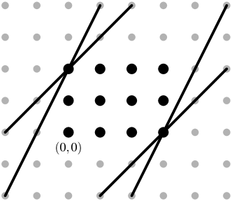
Figure 1: At corners of the reconstruction lattice, there can be local dependencies between line sums in two or more directions.

There is a strong analogy between the concept of dependencies between line sums in discrete tomography, and so-called consistency conditions in continuous tomography. Ludwig [18] and Helgason [12] described a set of relations between the projections of a continuous function defined on $\mathbb{R}^{2}$. Moreover, if a set of one-dimensional functions satisfies these relations, this is also a sufficient condition for correspondence to a projected function.

In the remainder of this paper, we provide a characterization of the dependencies between projections in discrete tomography, based on our algebraic framework. As dependencies indicate relations that must hold for any set of projections, they provide a necessary condition for the consistency problem. We prove that for a particular class of discrete tomography problems, a set of projections satisfies the dependency relations if and only if it corresponds to a table. This leads to a discrete analogon of the consistency conditions from continuous tomography.

3 Algebraic framework

In this section we introduce the basic concepts and definitions used in our algebraic formulation of discrete tomography. For a thorough introduction to terminology and concepts of Algebra, we refer to [17]. The Appendix of this paper covers some of the properties used in detail.

Let $A\subset\mathbb{Z}^{2}$ be non-empty and let $k$ be a commutative ring that is not the zero ring. We let

$$T(A,k)={k}^{({A})}=\left\{{f:A\rightarrow k\mid f(x)=0\mbox{ for all but finitely many $x\in A$}}\right\}$$

be the space of $k$-valued tables on $A$. It is a free $k$-module with a basis indexed by the elements of $A$. We will identify the elements of $A$ with the elements of this basis.

Let $d\in\mathbb{Z}^{2}\setminus\left\{{0}\right\}$ be a direction and $p\in\mathbb{Z}^{2}$ be a point. Recall that the (lattice) line through $p$ in the direction $d$ is the set $\left\{{p+\lambda d\mid\lambda\in\mathbb{Z}}\right\}$. Two points $p$ and $q$ are on the same line in direction $d$ precisely if they differ by an integer multiple of $d$. The quotient group $\mathbb{Z}^{2}/\left\langle{d}\right\rangle$ therefore parametrises all the lines in the direction $d$. For $A\subset\mathbb{Z}^{2}$ write $\mathcal{L}_{d}(A)$ for the image of $A$ in $\mathbb{Z}^{2}/\left\langle{d}\right\rangle$, i.e. the set of lines in the direction $d$ that intersect $A$.

We call $(a,b)\in\mathbb{Z}^{2}\setminus\left\{{0}\right\}$ with $\mathrm{gcd}\left({a,b}\right)=1$ a primitive direction. Whenever $d$ is a primitive direction, the quotient $\mathbb{Z}^{2}/\left\langle{d}\right\rangle$ is isomorphic to $\mathbb{Z}$. This means we can label the lines in direction $d$ with integers, starting with $0$ for the line through the origin.

We fix once and for all pairwise independent directions $d_{1},\ldots,d_{t}\in\mathbb{Z}^{2}\setminus\left\{{0}\right\}$ and write $\mathcal{L}_{i}(A)=\mathcal{L}_{d_{i}}(A)$ for the lines in direction $d_{i}$ that meet $A$. Let

$$L_{i}(A,k)={k}^{({\mathcal{L}_{i}(A)})}$$

be the space of potential line sums in direction $d_{i}$ and let

$$L(A,k)=\bigoplus_{i=1}^{t}L_{i}(A,k)$$

be the full space of potential line sums. These are all free $k$-modules. A basis for $L_{i}(A,k)$ is given by $\mathcal{L}_{i}(A)$ and so a basis for $L(A,k)$ is given by $\mathcal{L}(A):=\coprod_{i=1}^{t}\mathcal{L}_{i}(A)$.

Definition 3.1.

The line sum map

$$\sigma_{A,k}:T(A,k)\mathop{\longrightarrow}\limits L(A,k)$$

is defined as the $k$-linear map that sends $x\in A$ to the vector $(\ell_{i})_{i=1}^{t}$, where $\ell_{i}\in\mathcal{L}_{i}(A)$ is the line in direction $d_{i}$ through $x$.

The line sum map is the direct sum of the component maps $\sigma_{i,A,k}:T(A,k)\rightarrow L_{i}(A,k)$.

The kernel of the line sum map,

$$\mathrm{ker}\left({\sigma_{A,k}}\right)=\left\{{t\in T(A,k)\mid\sigma_{A,k}(t)=0}\right\},$$

identifies the space of switching components of the discrete tomography problem: two tables have the same vector of line sums if and only if they differ by an element of $\mathrm{ker}\left({\sigma_{A,k}}\right)$. We will use the cokernel

$$\mathrm{cok}\left({\sigma_{A,k}}\right)={L(A,k)}\big{/}\raisebox{-2.15277pt}{$\mathrm{im}\left({\sigma_{A,k}}\right)$}$$

to gain insight in the structure of the set of possible line sums of tables within the full space of potential line sums. In particular, the cardinality of the cokernel ‘measures’ the difference between these sets.

Definition 3.2.

A $k$-linear dependency between line sums is a $k$-linear map

$$r:L(A,k)\mathop{\longrightarrow}\limits k$$

such that $r\circ\sigma_{A,k}$ is the zero map.

Note that such a map gives rise to a map $\bar{r}:\mathrm{cok}\left({\sigma_{A,k}}\right)\rightarrow k$ and that conversely any $k$-linear map $\mathrm{cok}\left({\sigma_{A,k}}\right)\rightarrow k$ gives rise to a dependency. In other words, there is an inclusion

$$\mathrm{Hom}_{k}\left({\mathrm{cok}\left({\sigma_{A,k}}\right),k}\right)\subset\mathrm{Hom}_{k}\left({L(A,k),k}\right)$$

whose image is precisely the set of dependencies. We will write $\mathrm{Dep}\left({A,k}\right)$ for this subspace.

Remark 3.3.

The natural map

$$\begin{array}[]{rcccc}W&:&\mathrm{Hom}_{k}\left({L(A,k),k}\right)&\mathop{\longrightarrow}\limits&\left\{c:\mathcal{L}(A)\rightarrow k\right\}\\ &&\phi&\longmapsto&[\ell\mapsto\phi(\ell)]\end{array}$$

is a bijection.

For a $\phi\in\mathrm{Hom}_{k}\left({L(A,k),k}\right)$ we can think of $W(\phi)$ as the weight that $\phi$ assigns to each line in $\mathcal{L}(A)$. For dependencies this corresponds to the concept of a coefficient vector introduced in Section 2.1. If $r\in\mathrm{Dep}\left({A,k}\right)$ is a dependency then $W(r)$ corresponds to the vector $c$ from Definition 2.2.

The next lemma gives an example of the link between algebraic properties of the cokernel and questions concerning the discrete tomography problem.

Lemma 3.4.

Let $A\subset\mathbb{Z}^{2}$ and let $k$ be a commutative ring that is not the zero ring. Suppose that $\mathrm{cok}\left({\sigma_{A,k}}\right)$ is a free $k$-module of finite rank $n$. Then $\mathrm{Dep}\left({A,k}\right)$ is also a free $k$-module of rank $n$ and for any $l\in L(A,k)$ we have $l\in\mathrm{im}\left({\sigma_{A,k}}\right)$ if and only if $d(l)=0$ for all $d\in\mathrm{Dep}\left({A,k}\right)$.

Proof.

Let $c_{1},\ldots c_{n}$ be a basis for $\mathrm{cok}\left({\sigma_{A,k}}\right)$. We can write any $x\in\mathrm{cok}\left({\sigma_{A,k}}\right)$ uniquely as $x_{1}c_{1}+\cdots+x_{n}c_{n}$. The maps $e_{i}:x\mapsto x_{i}$ are elements of $\mathrm{Dep}\left({A,k}\right)=\mathrm{Hom}_{k}\left({\mathrm{cok}\left({\sigma_{A,k}}\right),k}\right)$. We claim that the $e_{i}$ are a basis for $\mathrm{Dep}\left({A,k}\right)$. Let $r$ be in $\mathrm{Dep}\left({A,k}\right)$. For any $x=\sum x_{i}c_{i}$ in $\mathrm{cok}\left({\sigma_{A,k}}\right)$ we have

$$r(x)=d(\sum x_{i}c_{i})=\sum x_{i}r(c_{i}).$$

Put $r_{i}=r(c_{i})$. Then we have $r=\sum r_{i}e_{i}$. So the $e_{i}$ generate $\mathrm{Dep}\left({A,k}\right)$. Note that the $r_{i}$ are uniquely determined by $r$. We conclude that the $e_{i}$ are a basis of $\mathrm{Dep}\left({A,k}\right)$.

Note that for all $x\in\mathrm{cok}\left({\sigma_{A,k}}\right)$, we have $x=\sum e_{i}(x)c_{i}$, so if $d(x)=0$ for all $d\in\mathrm{Dep}\left({A,k}\right)$, then $x=0$. When we apply this to $x=\bar{l}$ for some $l\in L(A,k)$, we see that $r(l)=0$ for all $r\in\mathrm{Dep}\left({A,k}\right)$ if and only if $\bar{l}=0$, i.e. $l\in\mathrm{im}\left({\sigma_{A,k}}\right)$. ∎

The lemma that we have just proved can be interpreted as follows. Whenever we find for some $A$ that $\mathrm{cok}\left({\sigma_{A,k}}\right)$ is a free $k$-module of finite rank, we have the following: A vector of potential line sums comes from a table precisely if it satisfies all dependencies. As the space of dependencies is also free and of finite rank, it in fact suffices to check finitely many dependencies.

4 The global case

In this section we consider the case $A=\mathbb{Z}^{2}$. We will show that in this case, the objects defined in the previous section have the structure of rings and modules, and their homomorphisms. This allows us to completely describe the kernel and cokernel of the line sum map.

The following three $k$-modules are isomorphic in a natural way:

$$T(\mathbb{Z}^{2},k)\qquad\cong\qquad k[\mathbb{Z}^{2}]\qquad\cong\qquad k[u,u^{-1},v,v^{-1}].$$

For some basic properties of group rings such as $k[\mathbb{Z}^{2}]$, see the appendix of this article. The isomorphisms are

$$\begin{array}[]{ccc}T(\mathbb{Z}^{2},k)&\mathop{\longrightarrow}\limits&k[\mathbb{Z}^{2}]\\ [c:\mathbb{Z}^{2}\rightarrow k]&\longmapsto&\sum_{x\in\mathbb{Z}^{2}}c(x)x\end{array}$$

and

$$\begin{array}[]{ccc}k[\mathbb{Z}^{2}]&\mathop{\longrightarrow}\limits&k[u,u^{-1},v,v^{-1}]\\ \sum_{x\in\mathbb{Z}^{2}}\lambda_{x}x&\longmapsto&\sum_{(a,b)\in\mathbb{Z}^{2}}\lambda_{(a,b)}u^{a}v^{b}.\end{array}$$

Note that $k[\mathbb{Z}^{2}]$ and $k[u,u^{-1},v,v^{-1}]$ are both $k$-algebras and that the second isomorphism is an isomorphism of $k$-algebras. We also view $T(\mathbb{Z}^{2},k)$ as a $k$-algebra via these isomorphisms.

In the same way there is a natural isomorphism of $k$-modules

$$L_{i}(\mathbb{Z}^{2},k)\cong k\left[{\mathbb{Z}^{2}}\big{/}\raisebox{-2.15277pt}{$\left\langle{d_{i}}\right\rangle$}\right]$$

which puts a ring structure on the spaces of potential line sums. By Lemma A.2 we have an isomorphism $k[\mathbb{Z}^{2}/\left\langle{d_{i}}\right\rangle]\cong k[\mathbb{Z}^{2}]/(d_{i}-1)$. Viewed in this way, the line sum map $\sigma_{i,\mathbb{Z}^{2},k}:T(\mathbb{Z}^{2},k)\rightarrow L_{i}(\mathbb{Z}^{2},k)$ is the quotient map

$$k[\mathbb{Z}^{2}]\rightarrow{k[\mathbb{Z}^{2}]}\big{/}\raisebox{-2.15277pt}{$(d_{i}-1)$}.$$

Taking sums, we find a $k$-algebra structure on $L(\mathbb{Z}^{2},k)$ such that the line sum map $\sigma_{\mathbb{Z}^{2},k}:T(\mathbb{Z}^{2},k)\rightarrow L(\mathbb{Z}^{2},k)$ is a $k$-algebra map which is the direct sum of quotient maps. We will now study the structure of these quotient maps from an algebraic perspective using the ideas outlined in the last part of the appendix.

Lemma 4.1.

Let $d,e\in\mathbb{Z}^{2}$ be independent directions. Then $d-1$ is weakly coprime (see A.6 in the appendix) to $e-1$ in $k[\mathbb{Z}^{2}]$.

Proof.

By Lemma A.2 we can see $k[\mathbb{Z}^{2}]/(d-1)$ as the group ring $k[\mathbb{Z}^{2}/\left\langle{d}\right\rangle]$. Suppose we have

$$f=\sum_{x\in\mathbb{Z}^{2}/\left\langle{d}\right\rangle}f_{x}x\in k\left[{\mathbb{Z}^{2}}\big{/}\raisebox{-2.15277pt}{$\left\langle{d}\right\rangle$}\right]$$

such that $(e-1)f=0$. When we expand

$$0=(e-1)f=\sum_{x\in\mathbb{Z}^{2}/\left\langle{d}\right\rangle}(f_{x-e}-f_{x})x,$$

we see that $f_{x+ke}=f_{x}$ for all $x\in\mathbb{Z}^{2}/\left\langle{d}\right\rangle$ and $k\in\mathbb{Z}$. As $d$ and $e$ are independent, all $x+ke$ are different in $\mathbb{Z}^{2}/\left\langle{d}\right\rangle$. We conclude that we must have $f_{x}=0$ for all $x\in\mathbb{Z}^{2}/\left\langle{d}\right\rangle$, as only finitely many coefficients of $f$ are non-zero. ∎

Theorem 4.2.

The kernel of $\sigma_{\mathbb{Z}^{2},k}$ is given by

$$\mathrm{ker}\left({\sigma_{\mathbb{Z}^{2},k}}\right)=(d_{1}-1)\cdots(d_{t}-1)k[\mathbb{Z}^{2}].$$

The cokernel $\mathrm{cok}\left({\sigma_{\mathbb{Z}^{2},k}}\right)$ is a free $k$-module of rank

$$\sum_{1\leq i<j\leq t}|\!\det(d_{i},d_{j})|.$$

Proof.

By Lemma 4.1, $d_{i}-1$ is weakly coprime to $d_{j}-1$ in $k[\mathbb{Z}^{2}]$ whenever $i\neq j$. So we can apply Theorem A.9 to the map

$$\sigma_{\mathbb{Z}^{2},k}:k[\mathbb{Z}^{2}]\mathop{\longrightarrow}\limits\bigoplus_{i=0}^{t}{\mathbb{Z}^{2}}\big{/}\raisebox{-2.15277pt}{$d_{i}-1$}.$$

This immediately gives us the formula for the kernel given in the theorem. For the cokernel, we note that by Lemma A.2 we have

$${k[\mathbb{Z}^{2}]}\big{/}\raisebox{-2.15277pt}{$(d_{i}-1,d_{j}-1)$}=k\left[{\mathbb{Z}^{2}}\big{/}\raisebox{-2.15277pt}{$\left\langle{d_{i},d_{j}}\right\rangle$}\right],$$

which is a free $k$-module of rank $|\det(d_{i},d_{j})|$. In particular, all the successive quotients of the filtration on the cokernel are free $k$-modules. Therefore all the quotients are split (see, e.g., [17, Ch. III.3, Prop. 3.2]) and we conclude that

$$\mathrm{cok}\left({\sigma_{\mathbb{Z}^{2},k}}\right)\cong\bigoplus_{1\leq i<j\leq t}k\left[{\mathbb{Z}^{2}}\big{/}\raisebox{-2.15277pt}{$\left\langle{d_{i},d_{j}}\right\rangle$}\right].$$

∎

This result leads to a (partial) discrete analogon of the Helgason-Ludwig consistency conditions from continuous tomography, providing a necessary and sufficient condition for consistency of a vector of potential line sums:

Corollary 4.3.

A vector of potential line sums in $L(\mathbb{Z}^{2},k)$ comes from a table in $T(\mathbb{Z}^{2},k)$ if and only if it satisfies all dependencies. Moreover, we only have to check this for a set of $\sum_{1\leq i<j\leq t}|\!\det(d_{i},d_{j})|$ independent dependencies.

Proof.

Theorem 4.2 shows that we can apply Lemma 3.4 to the global cokernel. ∎

Looking at example 2.2 we compute $\sum_{1\leq i<j\leq 4}|\!\det(d_{i},d_{j})|=7$. This tells us that the list of 7 independent dependencies we had is complete, in the sense that at least when $k$ is a field, they will form a basis of $\mathrm{Dep}\left({\mathbb{Z}^{2},k}\right)$.

For a full discrete analogon of the continuous consistency conditions, one should also provide a charaterization of the structure of the individual dependencies. The next section provides additional insight into the coefficient structure of the dependencies.

5 The global line sum map as an extension of rings

We now focus our attention more on the ring theoretic aspect of the line sum map. We can view $L(\mathbb{Z}^{2},k)$ as an extension of its subring $\mathrm{im}\left({\sigma_{\mathbb{Z}^{2},k}}\right)$. Both these rings have relative dimension $1$ over $k$. This is a situation that has been extensively studied because of its relation to Algebraic Number Theory. An important object in this context is the conductor of the extension, the largest ideal of $L(\mathbb{Z}^{2},k)$ that is also an ideal of $\mathrm{im}\left({\sigma_{\mathbb{Z}^{2},k}}\right)$.

Lemma 5.1.

Put $D_{i}=\prod_{j\neq i}(d_{j}-1)$. The conductor of $L(\mathbb{Z}^{2},k)$ over $\mathrm{im}\left({\sigma_{\mathbb{Z}^{2},k}}\right)$ is given by

$$\mathfrak{f}_{k}=\overline{D_{1}}{k[\mathbb{Z}^{2}]}\big{/}\raisebox{-2.15277pt}{$d_{1}-1$}\oplus\cdots\oplus\overline{D_{t}}{k[\mathbb{Z}^{2}]}\big{/}\raisebox{-2.15277pt}{$d_{t}-1$}.$$

Proof.

Note that $D_{i}$ reduces to $0$ in $k[\mathbb{Z}^{2}]/(d_{j}-1)$ for all $j\neq i$. We conclude that the ideal $(D_{1},\ldots,D_{t})$ of $k[\mathbb{Z}^{2}]$ is mapped by $\sigma_{\mathbb{Z}^{2},k}$ onto $\mathfrak{f}_{k}$. In particular, this implies that $\mathfrak{f}_{k}$ is indeed an $\mathrm{im}\left({\sigma_{\mathbb{Z}^{2},k}}\right)$ ideal.

Conversely, suppose $I\subset\mathrm{im}\left({\sigma_{\mathbb{Z}^{2},k}}\right)$ is an ideal that is also closed under multiplication by $L(\mathbb{Z}^{2},k)$. We want to show that $I\subset\mathfrak{f}_{k}$. Let $x=(x_{1},\dots,x_{t})\in I$. As $I$ is an $L(\mathbb{Z}^{2},k)$ ideal, we must also have $(0,\ldots,x_{i},\ldots,0)\in I$. As $I\subset\mathrm{im}\left({\sigma_{\mathbb{Z}^{2},k}}\right)$ there is an $\tilde{x}_{i}\in k[\mathbb{Z}^{2}]$ such that $\sigma_{\mathbb{Z}^{2},k}(\tilde{x}_{i})=(0,\ldots,x_{i},\ldots,0)$. We have $x=\sigma_{\mathbb{Z}^{2},k}(\tilde{x}_{1}+\cdots+\tilde{x}_{t})$, so we are done if we can show that $\tilde{x}_{i}$ is a multiple of $D_{i}$ for all $i$.

To show this, we apply Theorem 4.2 to the directions $d_{j}$ with $j\neq i$. Note that $\tilde{x}_{i}$ maps to $0$ under the line sum map in this case. The theorem tells us that the kernel of this map is generated by $D_{i}$, so that indeed $\tilde{x}_{i}$ is a multiple of $D_{i}$ for all $i$. ∎

Note that the quotient module $L(\mathbb{Z}^{2},k)/\mathfrak{f}_{k}$ is a free $k$-module of dimension $\sum_{i\neq j}|\det(d_{i},d_{j})|$. This is twice the dimension of $\mathrm{cok}\left({\sigma_{\mathbb{Z}^{2},k}}\right)=L(Z^{2},k)/\mathrm{im}\left({\sigma_{\mathbb{Z}^{2},k}}\right)$. We see that $\mathrm{im}\left({\sigma_{\mathbb{Z}^{2},k}}\right)$ sits precisely in the middle between $L(\mathbb{Z}^{2},k)$ and $\mathfrak{f}_{k}$. This is not a surprise, it happens in this situation whenever the rings are ‘sufficiently nice,’ e.g. when they are Gorenstein rings.

We have not yet fully explored the implications of this ring theoretic view for the structure of $\mathrm{cok}\left({\sigma_{\mathbb{Z}^{2},k}}\right)$, but we believe it warrants further investigation. To illustrate its use, we will derive the following result on the coefficient functions of dependencies in $\mathrm{Dep}\left({\mathbb{Z}^{2},k}\right)$.

For the remainder of this section, we assume that all the $d_{i}$ are primitive directions. This means that $\mathbb{Z}^{2}/\left\langle{d_{i}}\right\rangle$ is isomorphic to $\mathbb{Z}$. For the rest of this section we also fix isomorphisms $\mathbb{Z}^{2}/\left\langle{d_{i}}\right\rangle\cong\mathbb{Z}$. What this means is that the lines in each direction $d_{i}$ can be numbered in sequence. The choice of isomorphisms comes down to picking whether we number from left to right or the other way around.

Recall from Remark 3.3 that a dependency $r\in\mathrm{Dep}\left({Z^{2},k}\right)$ can be represented by a function $W(r)$ from $\mathcal{L}(\mathbb{Z}^{2})$ to $k$. From the choices we have just made, $\mathcal{L}(\mathbb{Z}^{2})$ is identified with $t$ copies of $\mathbb{Z}$. This means that to represent a dependency by a set of $t$ two-sided infinite sequences

$$W_{i}(r):\mathbb{Z}\mathop{\longrightarrow}\limits k.$$

Theorem 5.2.

With the assumptions above, each sequence $W_{i}(r)$ satisfies a non-trivial linear recurrence relation that does not depend on $r$.

Proof.

The isomorphism $\mathbb{Z}^{2}/\left\langle{d_{i}}\right\rangle\cong\mathbb{Z}$ gives rise to an isomorphism

$${k[\mathbb{Z}^{2}]}\big{/}\raisebox{-2.15277pt}{$d_{i}-1$}\cong k\left[{Z^{2}}\big{/}\raisebox{-2.15277pt}{$\left\langle{d_{i}}\right\rangle$}\right]\cong k[x,x^{-1}]$$

of $L_{i}(\mathbb{Z}^{2},k)$ with the Laurent polynomial ring $k[x,x^{-1}]$. Write $\overline{D_{i}}=\sum_{n}a_{n}x^{n}$ in $k[x,x^{-1}]$.

Let $r\in\mathrm{Dep}\left({\mathbb{Z}^{2},k}\right)$ be a dependency. We consider the map $r_{i}:L_{i}(\mathbb{Z}^{2},k)\rightarrow k$ induced by $r$. As $\mathrm{im}\left({\sigma_{\mathbb{Z}^{2},k}}\right)$ is in the kernel of $r$, we have $\mathfrak{f}_{k}\subset\mathrm{ker}\left({r}\right)$. As $x\in k[x,x^{-1}]$ is a unit, we see that $x^{n}\overline{D_{i}}$ must be in $\mathrm{ker}\left({r_{i}}\right)$ for all integers $n$.

Write $c$ for the weight function $W_{i}(r)$ from $\mathbb{Z}$ to $k$. From the definitions, we have for all $n\in\mathbb{Z}$ that $r_{i}(x^{n})=c(n)$. Let $m\in Z$. Then we must have

$$0=r_{i}(x^{m}\overline{D_{i}})=r_{i}(\sum_{n}a_{n}x^{m+n})=\sum_{n}a_{n}c(m+n).$$

This is saying precisely what we want, namely that $c$ satisfies a linear recurrence relation whose coefficients are the $a_{n}$. Clearly, these $a_{n}$ do not depend on $r$, only on $D_{i}$ and maybe on $k$. ∎

In fact, one computes that for $i=1,\ldots t$ we have

$$\overline{D_{i}}=\prod_{j\neq i}(x^{\det(d_{i},d_{j})}-1).$$

From this, one easily sees that the leading and trailing coefficients of $\overline{D_{i}}$ are $\pm 1$. Therefore, no matter what $k$ is, the recurrence relation can be used to uniquely determine the sequence from any sufficiently large set of consecutive coefficients. In fact, all the coefficient functions can be expressed in a closed form

$$[W_{i}(r)](s)=f_{s\ \mathrm{mod}\ m}(s)$$

where the $f$ are polynomials. The maximal degrees of these polynomials and the value of $m$ depend only on the $d_{i}$ and the characteristic of $k$.

6 An example

We revisit the example from [11] that was discussed in Section 2.2. It concerns the directions $d_{1}=(1,0)$, $d_{2}=(0,1)$, $d_{3}=(1,1)$ and $d_{4}=(1,-1)$. For simplicity, we take $k=\mathbb{Q}$, but we will make some comments on how to deal with the case $k=\mathbb{Z}$.

We identify $T(\mathbb{Z}^{2},k)$ with $k[x,x^{-1},y,v^{-1}]$. Note that for each $i$, we have $\mathbb{Z}^{2}/\left\langle{d}\right\rangle\cong\mathbb{Z}$. We pick isomorphisms $L_{i}(\mathbb{Z}^{2},k)=k[z,z^{-1}]$ in such a way that the components of the line sum map are the maps $k[x,x^{-1},y,y^{-1}]\rightarrow k[z,z^{-1}]$ given by

$$\begin{array}[]{c|c|c|c}i&\mbox{map}&x\mapsto&y\mapsto\\ \hline\cr 1&r&1&z\\ 2&c&z&1\\ 3&t&z&z^{-1}\\ 4&u&z&z\end{array}$$

The line sum map is given by

$$\sigma=(r,c,t,u):k[x,x^{-1},y,y^{-1}]\mathop{\longrightarrow}\limits\left(k[z,z^{-1}]\right)^{4}$$

The maps $r,c,t$ and $u$ are related to the line sums described in Section 2.2 in a straightforward manner. Let $f$ and the $r_{i},c_{i},t_{i}$ and $u_{i}$ be as in that section. Put $F=\sum_{i,j}f(i,j)x^{i}y^{j}$. Then we have $r(F)=\sum_{i}r_{i}z^{i}$ and likewise for the other maps.

We compute

$$\begin{array}[]{lcl}D_{1}=(y-1)(xy-1)(xy^{-1}-1)&&r(D_{1})=-z^{-1}(z-1)^{3}\\ D_{2}=(x-1)(xy-1)(xy^{-1}-1)&&c(D_{2})=(z-1)^{3}\\ D_{3}=(x-1)(y-1)(xy^{-1}-1)&&t(D_{3})=(z-1)^{3}(z+1)\\ D_{4}=(x-1)(y-1)(xy-1)&&u(D_{4})=(z-1)^{3}(z+1)\end{array}$$

Let $M=M_{1}\oplus\cdots\oplus M_{4}$ be the quotient vector space

$$M=\frac{k[z,z^{-1}]}{r(D_{1})}\oplus\frac{k[z,z^{-1}]}{c(D_{2})}\oplus\frac{k[z,z^{-1}]}{t(D_{3})}\oplus\frac{k[z,z^{-1}]}{u(D_{4})}$$

and $\pi=(\pi_{1},\ldots,\pi_{4})$ be the quotient map $(k[z,z^{-1}])^{4}\rightarrow M$. As discussed in the previous section, there is a surjective map $M\rightarrow\mathrm{cok}\left({\sigma}\right)$. This means we can realize $\mathrm{Dep}\left({\mathbb{Z}^{2},k}\right)$ as a subspace of $\mathrm{Hom}\left({M,k}\right)$.

A basis for $\mathrm{Hom}\left({k[z,z^{-1}]/(z-1)^{3},k}\right)$ is given by the maps

$$v_{1}:z^{i}\mapsto 1\qquad v_{2}:z^{i}\mapsto i\qquad v_{3}:z^{i}\mapsto i^{2}.$$

Let $e:\mathbb{Z}\mapsto\mathbb{Z}$ be the map that sends $n$ to $0$ if $n$ is odd, and to $1$ if it is even. A basis for $\mathrm{Hom}\left({k[z,z^{-1}]/(z-1)^{3}(z+1),k}\right)$ is given by

$$w_{1}:z^{i}\mapsto e(i)\qquad w_{2}:z^{i}\mapsto 1-e(i)\qquad w_{3}:z^{i}\mapsto i\qquad w_{4}:z^{i}\mapsto i^{2}.$$

These maps together give a basis for $\mathrm{Hom}\left({M,k}\right)$ consisting of $14$ elements:

• $v_{1,1}$, $v_{1,2}$ and $v_{1,3}$ acting on the first coordinate;

• $v_{2,1}$, $v_{2,2}$ and $v_{2,3}$ acting on the second coordinate;

• $w_{1,1},\ldots,w_{1,4}$ acting on the third coordinate and

• $w_{2,1},\ldots,w_{2,4}$ acting on the fourth coordinate.

These maps correspond to the sums of line sums that also come up in Section 2.2. For example $v_{1,1}$ sends $F$ to $\sum_{i}r_{i}$ and $w_{2,3}$ sends $F$ to $\sum_{i}i^{2}u_{i}$.

The dependencies form a subvector space of $\mathrm{Hom}\left({M,k}\right)$ of dimension $7$. What we still have to do is to determine which linear combinations of $v_{i,j}$’s and $w_{i,j}$’s correspond to dependencies. One way to do this is to write down the restrictions coming from the fact that tables of the form $x^{i}y^{j}$ must be sent to $0$ by a dependency. We will see in Section 8 that we only have to check finitely many such tables before we have a complete set of restrictions.

Another way to find these restriction is to consider the compositions of the $v$’s and $w$’s with $\pi\circ\sigma$, i.e., the maps they induce in $\mathrm{Hom}\left({k[x,x^{-1},y,y^{-1}],k}\right)$. The dependencies are precisely those relations that go to $0$ under this composition. The maps we obtain in this way are

$$\begin{array}[]{c|ccc|c}\mbox{map}&x^{i}y^{j}\mapsto&&\mbox{map}&x^{i}y^{j}\mapsto\\ \hline\cr v_{1,1}&1&&v_{2,1}&1\\ v_{1,2}&i&&v_{2,1}&j\\ v_{1,3}&i^{2}&&v_{2,1}&j^{2}\\ w_{1,1}&e(i-j)&&w_{2,1}&e(i+j)\\ w_{1,2}&1-e(i-j)&&w_{2,2}&1-e(i+j)\\ w_{1,3}&i-j&&w_{2,3}&i+j\\ w_{1,3}&(i-j)^{2}&&w_{2,3}&(i+j)^{2}\end{array}$$

From this table, one easily reads off a basis for the dependencies. For example, we can take

$$v_{1,1}=v_{2,1} = w_{1,1}+w_{1,2}=w_{2,1}+w_{2,2}$$

$$w_{1,1} = w_{2,1}$$

$$v_{1,2}-v_{2,2} = w_{1,3}$$

$$v_{1,2}+v_{2,2} = w_{2,3}$$

$$2v_{1,3}+2v_{2,3} = w_{1,4}+w_{2,4}.$$

These correspond to the dependencies described in Section 2.2.

If we want to write down a basis for the dependencies not over $\mathbb{Q}$ but over $\mathbb{Z}$ or some other ring, we have to be a little more careful. The maps $v_{1},\ldots v_{3}$ do not form a basis of $\mathrm{Hom}\left({k[z,z^{-1}]/(z-1)^{3},k}\right)$ if $k=\mathbb{Z}$. The map sending $z^{i}$ to $\frac{1}{2}i(i-1)$ is in this module, but it is equal to $\frac{1}{2}(v_{3}-v_{2})$, which is not a $\mathbb{Z}$-linear combination of the $v$’s.

A basis that works regardless of the ring $k$ is found as follows. Note that

$${k[z,z^{-1}]}\big{/}\raisebox{-2.15277pt}{$(z-1)^{3}$}=k\cdot 1\oplus k\cdot z\oplus k\cdot z^{2}$$

This choise of a basis also gives a basis for the $k$-dual. This basis works independently of $k$. The price we pay for this more general approach is that the formulas that come out aren’t as nice, making it harder to find the dependencies by hand. The linear algebra involved does not become more difficult.

7 The comparison sequence

Let $A\subset B\subset\mathbb{Z}^{2}$. Our aim in this section is to compare the kernels and cokernels of $\sigma_{A,k}$ and $\sigma_{B,k}$.

Put $T(B/A,k)={k}^{({B\setminus A})}$ and $L(B/A,k)=\bigoplus_{i=1}^{t}{k}^{({\mathcal{L}_{i}(B)\setminus\mathcal{L}_{i}(A)})}$. Looking at the bases for the spaces involved, it is clear that there are direct sum decompositions $T(B,k)=T(A,k)\oplus T(B/A,k)$ and $L(B,k)=L(A,k)\oplus L(B/A,k)$.

This means we can represent $\sigma_{B,k}$ as a two-by-two matrix of $k$-linear maps

$$\sigma_{B,k}=\left(\begin{matrix}p&q\\ r&s\end{matrix}\right),$$

where $p:T(A,k)\rightarrow L(A,k)$, $q:T(B/A,k)\rightarrow L(A,k)$, $r:T(A)\rightarrow L(B/A,k)$, and $s:T(B/A,k)\rightarrow L(B/A,k)$ are the restrictions and projections of $\sigma_{B,k}$ to the appropriate subspaces. The usual matrix multiplication rule

$$\left(\begin{matrix}p&q\\ r&s\end{matrix}\right)\left(\begin{matrix}x\\ y\end{matrix}\right)=\left(\begin{matrix}u\\ v\end{matrix}\right)$$

holds when we have $x\in T(A,k)$, $y\in T(B/A,k)$, $u\in L(A,k)$, and $v\in L(B/A,k)$ such that $\sigma_{B,k}(x\oplus y)=u\oplus v$.

As $L(B/A,k)$ consists precisely of those lines through $B$ that do not intersect $A$, we have $r=0$. Similarly, $p$ is just the map sending tables on $A$ to their line sums, so $p=\sigma_{A,k}$. The other two maps, $q$ and $s$ encode interesting information about the relative situation, so we will give them more descriptive names

$$\sigma_{B/A,k}:T(B/A,k)\mathop{\longrightarrow}\limits L(B/A,k)\quad\mbox{(the \emph{relative line sum map})}$$

and

$$\delta_{B/A,k}:T(B/A,k)\mathop{\longrightarrow}\limits L(A,k)\quad\mbox{(the \emph{interference map})}.$$

Lemma 7.1 (The comparison sequence).

There is a long exact sequence

$$\begin{array}[]{l}0\rightarrow\mathrm{ker}\left({\sigma_{A,k}}\right)\rightarrow\mathrm{ker}\left({\sigma_{B,k}}\right)\rightarrow\mathrm{ker}\left({\sigma_{B/A,k}}\right)\\ \quad\rightarrow\mathrm{cok}\left({\sigma_{A,k}}\right)\rightarrow\mathrm{cok}\left({\sigma_{B,k}}\right)\rightarrow\mathrm{cok}\left({\sigma_{B/A,k}}\right)\rightarrow 0.\end{array}$$

The map $\overline{\delta_{B/A,k}}:\mathrm{ker}\left({\sigma_{B/A,k}}\right)\rightarrow\mathrm{cok}\left({\sigma_{A,k}}\right)$ comes from the interference map $\delta_{B/A,k}$ defined above.

Proof.

This is an application of the Snake Lemma (See, for example, [17, Ch. III.9, Lemma 9.1.]). ∎

The extension $B/A$ is called non-interfering if it satisfies the following (equivalent) conditions:

1. the map $\overline{\delta_{B/A,k}}$ is the zero map;

2. the map $\mathrm{ker}\left({\sigma_{B,k}}\right)\rightarrow\mathrm{ker}\left({\sigma_{B/A,k}}\right)$ is surjective;

3. the map $\mathrm{cok}\left({\sigma_{A,k}}\right)\rightarrow\mathrm{cok}\left({\sigma_{B,k}}\right)$ is injective.

8 Finite, convex $A$

A subset $C\subset\mathbb{R}^{2}$ is called convex if for any $x,y\in C$ the line segment between $x$ and $y$ is completely contained in $C$. The convex hull of a subset $S\subset\mathbb{R}^{2}$ is the smallest convex subset $C$ of $\mathbb{R}^{2}$ containing $S$. We write $H(S)$ for the convex hull of $S$. We call $A\subset\mathbb{Z}^{2}$ convex if $A=H(A)\cap\mathbb{Z}^{2}$.

We call $C\subset\mathbb{R}^{2}$ a convex polygon if $C=H(S)$ for some finite $S\subset\mathbb{R}^{2}$. The set of corners of a convex polygon $C$ is the smallest set $S$ such that $H(S)=C$.

Let $C_{1},C_{2}\subset\mathbb{R}^{2}$ be convex polygons. Then

$$C_{1}+C_{2}=\left\{{c_{1}+c_{2}\mid c_{1}\in C_{1},c_{2}\in C_{2}}\right\}$$

is also a convex polygon. Let $s$ be a corner of $C_{1}+C_{2}$. Then $s$ can be written in a unique way as $s_{1}+s_{2}$ with $s_{1}\in C_{1}$ and $s_{2}\in C_{2}$. Moreover, $s_{1}$ and $s_{2}$ are corners of $C_{1}$ and $C_{2}$ respectively.

Let $f\in k[\mathbb{Z}^{2}]$ and write $f=\sum_{x\in\mathbb{Z}_{2}}f_{x}x$. Then the support of $f$ is the set

$$\mathrm{supp}{\left({f}\right)}=\left\{{x\in\mathbb{Z}^{2}\mid f_{x}\neq 0}\right\}.$$

Note that $\mathrm{supp}{\left({f}\right)}$ is always a finite set. The polygon of $f$ is

$$P(f)=H(\mathrm{supp}{\left({f}\right)}).$$

It is a convex polygon. Let $s$ be a corner of $P(f)$, then we say that $s$ is a strong corner of $P(f)$ if $f_{s}$ is not a zero divisor. We say that $f$ has strong corners if all corners of $P(f)$ are strong.

Lemma 8.1.

Let $f,g\in k[\mathbb{Z}^{2}]$ and suppose that $f$ has strong corners. Then

$$P(fg)=P(f)+P(g).$$

If $g$ also has strong corners, $fg$ has strong corners.

Proof.

The inclusion $P(fg)\subset P(f)+P(g)$ is obvious. For the other inclusion, suppose that $s$ is a corner of $P(f)+P(g)$. Then the coefficient of $fg$ at $s$ is

$$\sum_{a+b=s}f_{a}g_{b}=f_{s_{f}}g_{s_{g}},$$

where $s_{f}$ and $s_{g}$ are the unique corners of $P(f)$ and $P(g)$ respectively such that $s=s_{f}+s_{g}$. We see that this coefficient is non-zero as $f_{s_{f}}$ is not a zero divisor, so $s\in P(fg)$. This shows that $P(f)+P(g)\subset P(fg)$. Moreover, if $g$ also has strong corners, $g_{s_{g}}$ is also not a zero divisor and so $f_{s_{f}}g_{s_{g}}$ is not a zero divisor. ∎

Lemma 8.2.

The generator of $\mathrm{ker}\left({\sigma_{\mathbb{Z}^{2},k}}\right)$,

$$D=(d_{1}-1)\cdots(d_{t}-1),$$

has strong corners. Moreover, $\Delta=P(D)$ does not depend on $k$.

Proof.

The polygon of $d_{i}-1$ is a $2$-gon with coefficients $\pm 1$ at the corners, so $d_{i}-1$ has strong corners. The previous lemma then implies that $D$ has strong corners.

Let $D_{\mathbb{Z}}=(d_{1}-1)\cdots(d_{t}-1)\in\mathbb{Z}[\mathbb{Z}^{2}]$, then $D$ is the image of $D_{\mathbb{Z}}$ under the natural map $\mathbb{Z}[\mathbb{Z}^{2}]\rightarrow k[\mathbb{Z}^{2}]$. Note that the corners of $D_{\mathbb{Z}}$ will have coefficients $\pm 1$, as this is true for all the factors $d_{1}-1$. This means that $P(D)=P(D_{\mathbb{Z}})$ does not depend on $k$, as $\pm 1$ never maps to $0$ in $k$. ∎

Theorem 8.3.

Let $A\subset\mathbb{Z}^{2}$ be finite and convex. Then $\mathrm{ker}\left({\sigma_{A,k}}\right)$ and $\mathrm{cok}\left({\sigma_{A,k}}\right)$ are free $k$-modules of finite rank. The ranks of these modules do not depend on $k$.

Proof.

Note that $\sigma_{A,k}$ is the restriction of $\sigma_{\mathbb{Z}^{2},k}$ to $A$, and so we have

$$\mathrm{ker}\left({\sigma_{A,k}}\right)=\mathrm{ker}\left({\sigma_{\mathbb{Z}^{2},k}}\right)\cap T(A,k).$$

Using this, we compute

$$\begin{array}[]{rcl}\mathrm{ker}\left({\sigma_{A,k}}\right)&=&\mathrm{ker}\left({\sigma_{\mathbb{Z}^{2},k}}\right)\cap T(A,k)\\ &=&Dk[\mathbb{Z}^{2}]\cap T(A,k)\\ &=&\left\{{f\in Dk[\mathbb{Z}^{2}]\mid\mathrm{supp}{\left({f}\right)}\subset A}\right\}\\ &=&\left\{{f\in Dk[\mathbb{Z}^{2}]\mid P(f)\subset H(A)}\right\}\\ &=&\left\{{fD\mid f\in k[\mathbb{Z}^{2}],P(fD)\subset H(A)}\right\}\\ &=&\left\{{fD\mid f\in k[\mathbb{Z}^{2}],P(f)+\Delta\subset H(A)}\right\}.\end{array}$$

The latter is clearly a free $k$-module of finite rank with a basis indexed by the $x\in\mathbb{Z}^{2}$ such that $x+\Delta\subset H(A)$. By Lemma 8.2, this basis is independent of $k$. Therefore the rank of $\mathrm{ker}\left({\sigma_{A,k}}\right)$ does not depend on $k$.

This proves the result for the kernel. The result for the cokernel now follows from algebraic generalities. It suffices to show that $\mathrm{cok}\left({\sigma_{A,\mathbb{Z}}}\right)$ is a free $\mathbb{Z}$-module of finite rank, as taking cokernels commutes with taking tensor products (see e.g. [17, Ch. XVI.2, Prop. 2.6].) Since it is clearly finitely generated, we must show that it is torsion-free [17, Ch. I.8, Thm. 8.4]. We do this by comparing the ranks over $\mathbb{F}_{p}$ for $p$ prime to the rank over $\mathbb{Z}$.

From the sequence

$$0\rightarrow\mathrm{ker}\left({\sigma_{A,\mathbb{Z}}}\right)\rightarrow T(A,\mathbb{Z})\rightarrow L(A,\mathbb{Z})\rightarrow\mathrm{cok}\left({\sigma_{A,\mathbb{Z}}}\right)\rightarrow 0$$

we see that

$$\mathrm{rk}_{\mathbb{Z}}\left({\mathrm{cok}\left({\sigma_{A,\mathbb{Z}}}\right)}\right)=\mathrm{rk}_{\mathbb{Z}}\left({\mathrm{ker}\left({\sigma_{A,\mathbb{Z}}}\right)}\right)-\#A+\sum_{i=1}^{t}\#\mathcal{L}_{i}(A).$$

In the same way, we have for any prime $p$

$$\mathrm{dim}_{\mathbb{F}_{p}}\left({\mathrm{cok}\left({\sigma_{A,\mathbb{F}_{p}}}\right)}\right)=\mathrm{dim}_{\mathbb{F}_{p}}\left({\mathrm{ker}\left({\sigma_{A,\mathbb{F}_{p}}}\right)}\right)-\#A+\sum_{i=1}^{t}\#\mathcal{L}_{i}(A).$$

By the result about the kernel, we know that $\mathrm{rk}_{\mathbb{Z}}\left({\mathrm{ker}\left({\sigma_{A,\mathbb{Z}}}\right)}\right)=\mathrm{dim}_{\mathbb{F}_{p}}\left({\mathrm{ker}\left({\sigma_{A,\mathbb{F}_{p}}}\right)}\right)$. Using the formulas above this implies

$$\mathrm{rk}_{\mathbb{Z}}\left({\mathrm{cok}\left({\sigma_{A,\mathbb{Z}}}\right)}\right)=\mathrm{dim}_{\mathbb{F}_{p}}\left({\mathrm{cok}\left({\sigma_{A,\mathbb{F}_{p}}}\right)}\right).$$

But if $\mathrm{cok}\left({\sigma_{A,\mathbb{Z}}}\right)$ has any $p$-torsion, the $\mathbb{F}_{p}$-dimension would be strictly bigger. We conclude that $\mathrm{cok}\left({\sigma_{A,\mathbb{Z}}}\right)$ is torsion-free. ∎

Similar to the global case ($A=\mathbb{Z}^{2}$), this result allows to state a necessary and sufficient condition for consistency of a vector of potential line sums in the case of finite convex $A$:

Corollary 8.4.

Let $A\subset\mathbb{Z}^{2}$ be finite and convex. A vector of potential line sums in $L(A,k)$ comes from a table in $T(A,k)$ if and only if it satisfies all dependencies.

Proof.

Theorem 8.3 shows that we can apply Lemma 3.4 to the cokernel of the line sum map. ∎

9 Local and global dependencies

Let $A\subset\mathbb{Z}^{2}$. From the comparison sequence we have a map $\mathrm{cok}\left({\sigma_{A,k}}\right)\rightarrow\mathrm{cok}\left({\sigma_{\mathbb{Z}^{2},k}}\right).$ This map induces a map on the $k$-duals

$$\mathrm{Dep}\left({\mathbb{Z}^{2},k}\right)\mathop{\longrightarrow}\limits\mathrm{Dep}\left({A,k}\right).$$

We call the image of this map the global dependencies on $A$. When this map is injective, the dependencies on $\mathbb{Z}^{2}$ all restrict to different dependencies on $A$. Our intuition is that this should happen whenever $A$ is ‘sufficiently large.’

Lemma 9.1.

Suppose there is an $x\in\mathbb{Z}^{2}$ such that $x+\Delta\subset H(A)$. Then $\mathrm{cok}\left({\sigma_{A,k}}\right)\rightarrow\mathrm{cok}\left({\sigma_{\mathbb{Z}^{2},k}}\right)$ is surjective and so

$$\mathrm{Dep}\left({\mathbb{Z}^{2},k}\right)\mathop{\longrightarrow}\limits\mathrm{Dep}\left({A,k}\right)$$

is injective.

The geometric line through $p\in\mathbb{R}^{2}$ in the direction $d\in\mathbb{R}^{2}\setminus\left\{{0}\right\}$ is the set

$$\left\{{p+\lambda d\mid\lambda\in\mathbb{R}}\right\}\cap\mathbb{Z}^{2},$$

provided this set contains at least two points.

Let $d=(a,b)\in\mathbb{Z}^{2}\setminus\left\{{0}\right\}$ and put $g=\mathrm{gcd}\left({a,b}\right)$. Then any geometric line in direction $d$ is the union of $g$ lines. If $l$ is a geometric line in direction $d$ and $p,q\in H(l)$ are at least $\left|{d}\right|$ apart, then the line segment from $p$ to $q$ contains at least one point of every line through $l$.

Proof of Lemma 9.1.

Without loss of generality we restrict ourselves to $A=\Delta\cap\mathbb{Z}^{2}$. We want to show that for any $l\in L(\mathbb{Z}^{2},k)$, there is an $l^{\prime}\in L(A,k)$ that maps to the same element in $\mathrm{cok}\left({\sigma_{\mathbb{Z}^{2},k}}\right)$. That is, we must show

$$L(\mathbb{Z}^{2},k)=\mathrm{im}\left({\sigma_{\mathbb{Z}^{2},k}}\right)+L(A,k).$$

Recall that the conductor

$$\mathfrak{f}_{k}=\overline{D_{1}}{k[\mathbb{Z}^{2}]}\big{/}\raisebox{-2.15277pt}{$d_{1}-1$}\oplus\cdots\oplus\overline{D_{t}}{k[\mathbb{Z}^{2}]}\big{/}\raisebox{-2.15277pt}{$d_{t}-1$}$$

is the largest $L(\mathbb{Z}^{2},k)$ ideal that is contained in $\mathrm{im}\left({\sigma_{\mathbb{Z}^{2},k}}\right)$. It is therefore sufficient to show that $L(\mathbb{Z}^{2},k)=\mathfrak{f}_{k}+L(A,k)$, or, equivalently, that

$${k}^{({\mathcal{L}_{i}(A)})}\mathop{\longrightarrow}\limits{k[\mathbb{Z}^{2}]}\big{/}\raisebox{-2.15277pt}{$(d_{i}-1,D_{i})$}$$

is surjective for all $i$.

Let $l$ be a geometric line in direction $d_{i}$ such that $H(l)$ intersects $\Delta$. As we have $\Delta=P(D_{i})+P(d_{i}-1)$, the intersection is a segment of width at least $\left|{d_{i}}\right|$, so every line in the direction $d_{i}$ that lies in $l$ is in $\mathcal{L}_{i}(A)$. Let $S\subset\mathbb{Z}^{2}$ be the union of all the lines in $\mathcal{L}_{i}(A)$.

Note that $P(D_{i})$ does not have a side parallel to $d_{i}$, as all the directions are pairwise independent. It follows that $P(D_{i})$ has maximal points in the directions orthogonal to $d_{i}$. These points are nescesarily corners. The coefficients on these corners are $\pm 1$. It follows that for any $f\in k[\mathbb{Z}^{2}]$, there is a $g\in k[\mathbb{Z}^{2}]$ such that $\mathrm{supp}{\left({g}\right)}\subset S$ and $f-g\in D_{i}k[\mathbb{Z}^{2}]$.

By the above, this implies that

$${k}^{({\mathcal{L}_{i}(A)})}+\overline{D_{i}}{k[\mathbb{Z}^{2}]}\big{/}\raisebox{-2.15277pt}{$d_{i}-1$}={k[\mathbb{Z}^{2}]}\big{/}\raisebox{-2.15277pt}{$d_{i}-1$}$$

and so

$${k}^{({\mathcal{L}_{i}(A)})}\mathop{\longrightarrow}\limits{k[\mathbb{Z}^{2}]}\big{/}\raisebox{-2.15277pt}{$(d_{i}-1,D_{i})$}$$

is surjective. ∎

Let $A$ be finite and convex. We define the rounded part of $A$ to be the subset

$$A^{\prime}=\left(\bigcup(x+\Delta)\right)\cap\mathbb{Z}^{2}$$

where the union runs over all $x\in\mathbb{Z}^{2}$ such that $x+\Delta\subset H(A)$. We call $A$ rounded if it is non-empty and $A^{\prime}=A$.

Theorem 9.2.

Let $A$ be finite, convex and rounded. Then $\mathrm{cok}\left({\sigma_{A,k}}\right)$ is equal to $\mathrm{cok}\left({\sigma_{\mathbb{Z}^{2},k}}\right)$ and so we have

$$\mathrm{Dep}\left({A,k}\right)=\mathrm{Dep}\left({\mathbb{Z}^{2},k}\right).$$

Proof.

Note that by Lemma 9.1 the map

$$\mathrm{cok}\left({\sigma_{A,k}}\right)\mathop{\longrightarrow}\limits\mathrm{cok}\left({\sigma_{\mathbb{Z}^{2},k}}\right)$$

is surjective, so we just have to show it is injective. The strategy for this is to construct

$$A=A_{0}\subset A_{1}\subset A_{2}\subset\cdots$$

such that $A_{i+1}/A_{i}$ is non-interfering for all $i\geq 0$ and $\bigcup_{i\geq 0}A_{i}$ is all of $\mathbb{Z}^{2}$. Suppose that $l\in L(A,k)$ such that $l=\sigma_{\mathbb{Z}^{2},k}(t)$ for some $t\in T(\mathbb{Z}^{2},k)$. Then $t\in T(A_{i},k)$ for some $i$, so $l$ maps to $0$ in $\mathrm{cok}\left({\sigma_{A_{i},k}}\right)$. By the non-interference, $\mathrm{cok}\left({\sigma_{A,k}}\right)$ maps injectively to $\mathrm{cok}\left({\sigma_{A_{i},k}}\right)$, so it follows that $l$ maps to $0$ in $\mathrm{cok}\left({\sigma_{A,k}}\right)$, as required.

Pick a point $p$ in the interior of $H(A)$ in sufficiently general position (we will make this more precise later on). For $\lambda\in\mathbb{R}_{\geq 1}$ let $H(\lambda)$ be the point multiplication of the set $H(A)$ with factor $\lambda$ and center $p$. Let $A(\lambda)=H(\lambda)\cap\mathbb{Z}^{2}$. Note that the union of all $H(\lambda)$ is the entire plane, so we have

$$\bigcup\limits_{\lambda\geq 1}A(\lambda)=\mathbb{Z}^{2}.$$

As $\mathbb{Z}^{2}\subset\mathbb{R}^{2}$ is countable and discrete, the set of $\lambda$’s such that

$$A(\lambda)\neq\bigcup\limits_{1\leq\mu<\lambda}A(\mu)$$

is a countable and discrete subset of $\mathbb{R}_{\geq 1}$. Let $(\lambda_{i})_{i=0}^{\infty}$ be the sequence of these $\lambda$’s in increasing order. Put $A_{i}=A(\lambda_{i})$.

For all $\lambda\in\mathbb{R}_{\geq 1}$ one sees that

$$\bigcup\limits_{1\leq\mu<\lambda}H(\mu)$$

is the boundary of $H(\lambda)$. Therefore, any point in $A_{i+1}\setminus A_{i}$ is on the boundary of $H(\lambda_{i})$. This means that these points lie on finitely many line segments: the edges of the polygon $H(\lambda_{i+1})$.

In fact, by choosing the point $p$ outside a countable union of lines, one can ensure that for every $i$ there is a single edge $l_{i}$ of the polygon $H(\lambda_{i+1})$ such that all the points in $A_{i+1}\setminus A_{i}$ lie on that edge.

Suppose that $l_{i}$ does not lie in one of the directions $d_{1},\ldots d_{t}$. Then $\Delta$ has a maximal point $m$ in the direction orthogonal to $l_{i}$, which is a corner and so the corresponding coefficient of $D$ is $\pm 1$. Let $p\in A_{i+1}\setminus A_{i}$. As $A$ is rounded, the translate of $\Delta$ such that $m$ coincides with $p$ is contained entirely in $A_{i+1}$. It follows that the map

$$\mathrm{ker}\left({\sigma_{A_{i+1},k}}\right)\mathop{\longrightarrow}\limits{k}^{({A_{i+1}\setminus A_{i}})}$$

is surjective, so $A_{i+1}/A_{i}$ is non-interfering.

Suppose that $l_{i}$ lies in the direction $d_{j}$. The edge of $H(A)$ in direction $d_{j}$ is at least $\left|{d_{j}}\right|$ long, as $A$ is rounded. So the edge $l_{i}$ of $H(\lambda_{i+1})$ has length $\lambda_{i+1}|d_{j}|>|d_{j}|$. Therefore, every line in the direction $d_{j}$ that lies inside the geometric line containing $l_{i}$ meets $A_{i+1}$. Note that $\Delta$ has an edge in direction $d_{j}$ and that the intersection of $\mathrm{supp}{\left({D}\right)}$ with the geometric line through that edge consists precisely of the two corner points, both of which have coefficient $\pm 1$. These two points are adjacent points within the same line on that geometric line. As $A$ is rounded, every translate of $\Delta$ such that the edge in direction $d_{j}$ lies between on $l_{i}$, lies completely within $H(A)$. From these observations we can conclude that

$$\sigma_{A_{i+1}/A_{i},k}:T(A_{i+1}/A_{i},k)\mathop{\longrightarrow}\limits L(A_{i+1}/A_{i},k)$$

is onto and that its kernel is generated by the intersections of the correct translates of $D$ with $T(A_{i+1}/A_{i},k)$. Therefore the map

$$\mathrm{ker}\left({\sigma_{A_{i+1},k}}\right)\mathop{\longrightarrow}\limits\mathrm{ker}\left({\sigma_{A_{i+1}/A_{i},k}}\right)$$

is onto, that is, $A_{i+1}/A_{i}$ is non-interfering. ∎

Theorem 9.3.

Let $A$ be finite and convex and suppose that $A^{\prime}$ is non-empty. Then $\mathrm{Dep}\left({A,k}\right)$ decomposes in a natural way as a direct sum

$$\mathrm{Dep}\left({A,k}\right)=\mathrm{Dep}\left({\mathbb{Z}^{2},k}\right)\oplus\mathrm{Hom}_{k}\left({\mathrm{cok}\left({\sigma_{A/A^{\prime},k}}\right),k}\right).$$

We call the second summand the local dependencies on $A$.

Proof.

From the comparison sequence for $A/A^{\prime}$ we have

$$\mathrm{cok}\left({\sigma_{A^{\prime},k}}\right)\mathop{\longrightarrow}\limits_{f_{A/A^{\prime}}}\mathrm{cok}\left({\sigma_{A,k}}\right)\mathop{\longrightarrow}\limits\mathrm{cok}\left({\sigma_{A/A^{\prime},k}}\right)\mathop{\longrightarrow}\limits 0.$$

Lemma 9.1 shows $f_{A}:\mathrm{cok}\left({\sigma_{A,k}}\right)\rightarrow\mathrm{cok}\left({\sigma_{\mathbb{Z}^{2},k}}\right)$ is surjective and Theorem 9.2 shows $f_{A^{\prime}}:\mathrm{cok}\left({\sigma_{A^{\prime},k}}\right)\rightarrow\mathrm{cok}\left({\sigma_{\mathbb{Z}^{2},k}}\right)$ is bijective. Note that $f_{A^{\prime}}=F_{A}\circ f_{A/A^{\prime}}$. We conclude that $f_{A/A^{\prime}}$ is injective (so $A/A^{\prime}$ is non-interfering) and that $f_{A^{\prime}}^{-1}\circ f_{A}$ is a splitting map of $f_{A/A^{\prime}}$. It follows that

$$\mathrm{cok}\left({\sigma_{A,k}}\right)=\mathrm{cok}\left({\sigma_{A^{\prime},k}}\right)\oplus\mathrm{cok}\left({\sigma_{A/A^{\prime},k}}\right).$$

This implies the required result (recall that $\mathrm{Dep}\left({A^{\prime},k}\right)=\mathrm{Dep}\left({\mathbb{Z}^{2},k}\right)$.) ∎

10 Conclusions

To conclude this paper, we summarize the main results obtained within our algebraic framework, and their interpretation from the classical combinatorial perspective.

Lemma 3.4 relates an algebraic property of the cokernel of the line sum map to the consistency problem. Theorem 4.2 states that for the case $A=\mathbb{Z}^{2}$, the cokernel actually satisfies this property. In addition, a characterization of the switching components is provided for this case. This results in a strong statement concerning the consistency problem for the case $A=\mathbb{Z}^{2}$: a set of linesums corresponds to a table if and only if it satisfies a certain number of independent dependencies (Corollary 4.3). In Section 5, properties are derived on the structure of the coefficients in the separate dependencies. Section 6 relates the material from Section 3, 4 and 5 to the example from the Combinatorial DT literature, given in Section 2.2.

The next sections, starting with Section 7, focus on cases where $A$ is a true subset of $\mathbb{Z}^{2}$. A relative setup is introduced in Section 7, where a DT problem on a particular domain is related to a problem on a subset of that domain. In Sections 8 and 9, this relation is applied to describe the structure of line sums for finite convex sets. Corollary 4.3 provides a necessary and sufficient condition for consistency in the case of a finite, convex reconstruction domain. Theorem 9.2 shows that if $A$ is finite, convex and rounded, the dependencies are exactly those that also apply to the global case $A=\mathbb{Z}^{2}$. Finally, Theorem 9.3 considers the decomposition of the dependencies for the general finite convex case into global and local dependencies.

The results on the structure of dependencies between the line sums in discrete tomography problems can either be viewed as a collection of new research results, or as an illustration of the power of applying Ring Theory and Commutative Algebra to this combinatorial problem. We expect that a range of additional results can be obtained within the context of this algebraic framework.

Appendix A Tools from algebra

A.1 Group rings

We begin by recalling some results on group rings. See for example [17, Ch. II.3] for a short introduction or [19] for more results on these rings.

Definition A.1.

Let $k$ be a commutative ring and $G$ be a group. The group ring $k[G]$ is the $k$-algebra which as a $k$-module is the free with basis $G$,

$$k[G]=\bigoplus_{g\in G}k[g]$$

and whose multiplication is given by

$$\begin{array}[]{ccl}[g]\cdot[h]=[gh]&&\mbox{for all $g,h\in G$}\\ [g]\cdot\lambda=\lambda[g]&&\mbox{for all $g\in G$, $\lambda\in k$}.\end{array}$$

When there is no confusion possible we will drop the brackets around elements of $G$, writing a typical element of $k[G]$ simply as $\sum_{g\in G}\lambda_{g}g$ with $\lambda_{g}=0$ for almost all $g\in G$.

A ring homomorphism $k\mathop{\longrightarrow}\limits k^{\prime}$ induces a unique ring homomorphism

$$k[G]\mathop{\longrightarrow}\limits k^{\prime}[G].$$

A group homomorphism $G\mathop{\longrightarrow}\limits H$ induces a unique $k$-algebra homomorphism

$$k[G]\mathop{\longrightarrow}\limits k[H].$$

Lemma A.2.

Let $G$ be a group and $N$ be a normal subgroup. Let $I_{N}$ be the ideal of $k[G]$ generated by all elements of the form $n-1$ with $n\in N$. Then there is a short exact sequence

$$0\mathop{\longrightarrow}\limits I_{N}\mathop{\longrightarrow}\limits k[G]\mathop{\longrightarrow}\limits k[{G}\big{/}\raisebox{-2.15277pt}{$N$}]\mathop{\longrightarrow}\limits 0.$$

A.2 Filtrations

We continue with some generalities on filtrations.

Definition A.3.

Let $R$ be a commutative ring and $M$ an $R$-module. A filtration of $M$ is a collection of submodules

$$0=M_{0}\subset M_{1}\subset\cdots\subset M_{t}=M.$$

The quotient modules $M_{i+1}/M_{i}$ are called the successive quotients of the filtration.

Lemma A.4.

Let $R$ be a commutative ring and let $M^{\prime}$ and $M^{\prime\prime}$ be filtered $R$-modules. Suppose we have a short exact sequence

$$0\rightarrow M^{\prime}\rightarrow M\rightarrow M^{\prime\prime}\rightarrow 0.$$

Then $M$ admits a filtration whose successive quotients are those of $M^{\prime}$ followed by those of $M^{\prime\prime}$

Lemma A.5.

Let $R$ be a commutative ring, let $A,B$ and $C$ be $R$-modules and suppose $f:A\rightarrow B$ and $g:B\rightarrow C$ are injective morphisms. Then there is a short exact sequence

$$0\rightarrow\mathrm{cok}\left({f}\right)\rightarrow\mathrm{cok}\left({gf}\right)\rightarrow\mathrm{cok}\left({g}\right)\rightarrow 0.$$

A.3 Weak coprimality

The rest of this appendix is devoted to a generalisation of the concept of coprimality and the Chinese Remainder Theorem.

Definition A.6.

Let $R$ be a commutative ring and let $f,g\in R$. We say that $f$ is weakly coprime to $g$ if multiplication by $f$ is an injective map on ${R}\big{/}\raisebox{-2.15277pt}{$g$}$.

The common notion of coprimality, namely that the ideal $(f,g)$ generated by $f$ and $g$ be all of $R$, implies that multiplication by $f$ is a bijective map on ${R}\big{/}\raisebox{-2.15277pt}{$g$}$.

Lemma A.7.

Let $R$ be a commutative ring and let $f,g\in R$ such that $f$ is weakly coprime to $g$. Then there is a short exact sequence

$$0\rightarrow{R}\big{/}\raisebox{-2.15277pt}{$fg$}\rightarrow{R}\big{/}\raisebox{-2.15277pt}{$f$}\oplus{R}\big{/}\raisebox{-2.15277pt}{$g$}\rightarrow{R}\big{/}\raisebox{-2.15277pt}{$(f,g)$}\rightarrow 0.$$

Proof.

Straightforward verification.∎

If two elements are coprime in the common (strong) sense, then in the sequence above we have $R/(f,g)=0$, so the first map is an isomorphism. This fact is commonly refered to as the Chinese Remainder Theorem.

Lemma A.8.

Let $R$ be a commutative ring and let $f_{1},f_{2}$ and $g$ be in $R$. Suppose that $f_{1}$ and $f_{2}$ are weakly coprime to $g$. Then there is a short exact sequence

$$0\rightarrow{R}\big{/}\raisebox{-2.15277pt}{$(f_{1},g)$}\rightarrow{R}\big{/}\raisebox{-2.15277pt}{$(f_{1}f_{2},g)$}\rightarrow{R}\big{/}\raisebox{-2.15277pt}{$(f_{2},g)$}\rightarrow 0.$$

Proof.

Apply lemma A.5 to the multiplication by $f_{1}$ and by $f_{2}$ maps on $R/g$. ∎

Theorem A.9 (Weak Chinese Remainder Theorem).

Let $R$ be a commutative ring and let $x_{1},\cdots,x_{t}\in R$ have the property that $x_{i}$ is weakly coprime to $x_{j}$ whenever $i<j$. Then the natural map

$$\phi:{R}\big{/}\raisebox{-2.15277pt}{$x_{1}\cdots x_{t}$}\longrightarrow{R}\big{/}\raisebox{-2.15277pt}{$x_{1}$}\oplus\cdots\oplus{R}\big{/}\raisebox{-2.15277pt}{$x_{t}$}$$

is injective. Its cokernel admits a filtration whose successive quotients are isomorphic to ${R}\big{/}\raisebox{-2.15277pt}{$(x_{i},x_{j})$}$ for $1\leq i<j\leq t$.

Proof.

We proceed by induction on $t$. For $t=2$ the result is that of Lemma A.7. Let $t\geq 3$ and assume that the theorem holds for any smaller number of $x_{i}$’s.

We write $\phi$ as a composition of two maps. Let $\phi_{1}$ be the natural map

$$\phi_{1}:{R}\big{/}\raisebox{-2.15277pt}{$x_{1}\cdots x_{t}$}\mathop{\longrightarrow}\limits{R}\big{/}\raisebox{-2.15277pt}{$x_{1}\cdots x_{t-1}$}\oplus{R}\big{/}\raisebox{-2.15277pt}{$x_{t}$}$$

and $\phi_{2}$ the natural map

$$\phi_{2}:{R}\big{/}\raisebox{-2.15277pt}{$x_{1}\cdots x_{t-1}$}\mathop{\longrightarrow}\limits{R}\big{/}\raisebox{-2.15277pt}{$x_{1}$}\oplus\cdots\oplus{R}\big{/}\raisebox{-2.15277pt}{$x_{t-1}$}.$$

Then we have $\phi=(\phi_{2}\oplus\mathrm{id}_{R/x_{t}})\circ\phi_{1}$.

Note $x_{1}\cdots x_{t-1}$ is weakly coprime to $x_{t}$ as a composition of injective maps is again injective. So Lemma A.7 applies to $\phi_{1}$. In particular $\phi_{1}$ is injective. By the induction hypothesis, $\phi_{2}$ is also injective. We conclude that $\phi$ is injective.

By Lemma A.7 the cokernel of $\phi_{1}$ is $R/(x_{1}\cdots x_{t-1},x_{t})$. By repeatedly applying Lemma A.8, this module admits a filtration whose successive quotients are $R/(x_{i},x_{t})$ for $1\leq i\leq t-1$.

Furthermore, we have $\mathrm{cok}\left({\phi_{2}\oplus\mathrm{id}_{R/x_{t}}}\right)=\mathrm{cok}\left({\phi_{2}}\right)$, which by the induction hypothesis has a filtration whose successive quotients are isomorphic to $R/(x_{i},x_{j})$ with $1\leq i<j\leq t-1$.

We apply Lemma A.5 to the maps $\phi_{1}$ and $\phi_{2}\oplus\mathrm{id}_{R/x_{t}}$ and conclude that the cokernel of $\phi$ has the required filtration. ∎

References

- [1] A. Alpers and P. Gritzmann. On stability, error correction, and noise compensation in discrete tomography. SIAM J. Discrete Math., 20(1):227–239, 2006.
- [2] A. Alpers and R. Tijdeman. The two-dimensional Prouhet Tarry Escott problem. J. Number Theory, 123:403–412, 2007.
- [3] M. Baake, P. Gritzmann, C. Huck, B. Langfeld and K. Lord. Discrete tomography of planar model sets. Acta Cryst., 62:419–433, 2006.
- [4] E. Barcucci, A. Del Lungo, M. Nivat, and R. Pinzani. Reconstructing convex polyominoes from horizontal and vertical projections. Theoret. Comp. Sci., 155:321–347, 1996.
- [5] S. Brunetti, A. Del Lungo, F. Del Ristoro, A. Kuba, and M. Nivat. Reconstruction of 4- and 8-connected convex discrete sets from row and column projections. Linear Algebra Appl., 339:37–57, 2001.
- [6] D. Gale. A theorem on flows in networks. Pacific J. Math., 7:1073–1082, 1957.
- [7] R. J. Garnder and P. Gritzmann. Discrete tomography: determination of finite sets by X-rays. Trans. Am. Math. Soc., 349(6):2271–2295, 1997.
- [8] R. J. Gardner, P. Gritzmann, and D. Prangenberg. On the computational complexity of reconstructing lattice sets from their X-rays. Discrete Math., 202:45–71, 1999.
- [9] R. J. Gardner. Geometric Tomography, 2nd edition. Cambridge University Press, 2006.
- [10] P. Gritzmann and B. Langfeld. On the index of Siegel grids and its application to the tomography of quasicrystals. European J. Combin., 29:1894–1909, 2008.
- [11] L. Hajdu and R. Tijdeman. Algebraic aspects of discrete tomography. J. Reine Angew. Math., 534:119–128, 2001.
- [12] S. Helgason. The Radon transform. Birkhäuser, Boston, 1980.
- [13] G. T. Herman and A. Kuba, editors. Discrete Tomography: Foundations, Algorithms and Applications. Birkhäuser, Boston, 1999.
- [14] G. T. Herman and A. Kuba, editors. Advances in Discrete Tomography and its Applications. Birkhäuser, Boston, 2007.
- [15] J. R. Jinschek, K. J. Batenburg, H. A. Calderon, R. Kilaas, V. Radmilovic, and C. Kisielowski. 3-d reconstruction of the atomic positions in a simulated gold nanocrystal based on discrete tomography: Prospects of atomic resolution electron tomography. Ultramicroscopy, 108(6):589–604, 2007.
- [16] C. Kisielowski, P. Schwander, F. Baumann, M. Seibt, Y. Kim, and A. Ourmazd. An approach to quantitative high-resolution transmission electron microscopy of crystalline materials. Ultramicroscopy, 58:131–155, 1995.
- [17] Serge Lang. Algebra, volume 211 of Graduate Texts in Mathematics. Springer-Verlag, New York, third edition, 2002.
- [18] D. Ludwig. The radon transform on euclidean spaces. Commun. Pure Appl. Math., 19:49–81, 1966.
- [19] Donald S. Passman. The algebraic structure of group rings. Pure and Applied Mathematics. Wiley-Interscience [John Wiley & Sons], New York, 1977.
- [20] H. J. Ryser. Combinatorial properties of matrices of zeros and ones. Canadian J. Math., 9:371–377, 1957.
- [21] P. Schwander, C. Kisielowski, F. Baumann, Y. Kim, and A. Ourmazd. Mapping projected potential, interfacial roughness, and composition in general crystalline solids by quantitative transmission electron microscopy. Physical Review Letters, 71:4150–4153, 1993.
- [22] B. van Dalen. Dependencies between line sums. Master’s thesis, Leiden University, The Netherlands, 2007, http://www.math.leidenuniv.nl/scripties/DalenMaster.pdf.