On network coding for sum-networks

Abstract

A directed acyclic network is considered where all the terminals need to recover the sum of the symbols generated at all the sources. We call such a network a sum-network. It is shown that there exists a solvably (and linear solvably) equivalent sum-network for any multiple-unicast network, and thus for any directed acyclic communication network. It is also shown that there exists a linear solvably equivalent multiple-unicast network for every sum-network. It is shown that for any set of polynomials having integer coefficients, there exists a sum-network which is scalar linear solvable over a finite field $F$ if and only if the polynomials have a common root in $F$. For any finite or cofinite set of prime numbers, a network is constructed which has a vector linear solution of any length if and only if the characteristic of the alphabet field is in the given set. The insufficiency of linear network coding and unachievability of the network coding capacity are proved for sum-networks by using similar known results for communication networks. Under fractional vector linear network coding, a sum-network and its reverse network are shown to be equivalent. However, under non-linear coding, it is shown that there exists a solvable sum-network whose reverse network is not solvable.

I Introduction

Traditionally transmission of information has been considered similar to flow of commodity so that information is stored and forwarded by the intermediate nodes. The seminal work by Ahlswede et al. ([1]) showed that mixing or coding information at the intermediate nodes in a network may provide better throughput. Coding at the intermediate nodes has since been referred as network coding. For a multicast network, where the symbols generated at a single source are to be communicated to a set of terminals, it was shown that the capacity under network coding is the minimum of the min-cuts between the source and each of the terminals ([1]).

If the nodes perform linear operations, then the code is called a linear network code. It was shown by Li et al. ([2]) that linear network coding is sufficient to achieve the capacity of a multicast network. Koetter and Médard ([3]) proposed an algebraic formulation of the linear network code design problem and related this network coding problem to finding roots of a set of polynomials. Jaggi et al. ([4]) gave a polynomial time algorithm for solving this problem for a multicast network. Ho et al. ([5]) showed that even when the local coding coefficients are chosen randomly and in a distributed fashion, the multicast capacity can be achieved with high probability.

More general forms of network codes have been considered in the literature to allow more flexibility. If a block or vector of $n$ symbols is treated as a single symbol at all the nodes and edges, then a node takes a function of the incoming vectors to construct an outgoing vector on an edge. In each session, the receivers recover $n$-length vectors of symbols from their desired sources. Such a code is called a vector network code. Fractional network code is an even more general form of network code where the number of source symbols $k$ encoded in a block is possibly different from the block length $n$. Such a $(k,n)$ code communicates $k$ source symbols in $n$ use of the network, thus achieving the rate $k/n$ per network use.

A network is said to be solvable over an alphabet if there is a rate-$1$ network code over that alphabet which satisfies the demands of the terminals. For an underlying alphabet field, a network is said to be $k$-length vector linear solvable (resp. scalar linear solvable) if there is a $k$-length vector (resp. scalar) linear network coding solution for the network. Two networks ${\cal N}_{1}$ and ${\cal N}_{2}$ are said to be solvably equivalent (resp. linear solvably equivalent) if ${\cal N}_{1}$ is solvable (resp. solvable with linear codes) over some finite alphabet if and only if ${\cal N}_{2}$ is solvable (resp. solvable with linear codes) over the same alphabet.

Much of the subsequent work considered more general networks than multicast networks. Here a terminal requires the symbols generated at a subset of the sources. We call such networks where the aim is to communicate the source symbols to the appropriate terminals, as opposed to computation of functions of the source symbols at the terminals (which is the subject of this paper,) as communication networks. Designing a network code for a general communication network was shown to be an NP-hard problem ([6, 7]). It was shown in [8, 9] that for communication networks, scalar linear network coding is not sufficient in the sense that there may exist a vector linear network code though no scalar linear network code exists. Even vector linear network codes were shown to be insufficient by Dougherty et al. ([10]). They further showed in [11] that for every set of integer polynomial equations, there exists a directed acyclic network which is scalar linear solvable over a finite field if and only if the set of polynomial equations has a solution over the same finite field.

A network with some source-terminal pairs where every terminal wants the data generated at the respective source is called a multiple-unicast network. It was shown in [12] that from any communication network, one can construct a solvably equivalent multiple-unicast network. For a multiple-unicast network, the reverse network is obtained by reversing the direction of the edges and interchanging the roles of the sources and the terminals. It was shown in [13, 14] that a multiple-unicast network is linear solvable if and only if its reverse network is linearly solvable. However, it was shown in [14, 12] that there exists a multiple-unicast network which is solvable by a non-linear network code though its reverse network is not solvable.

In this paper, we consider a network with some sources $s_{1},s_{2},\cdots,s_{m}$ and some terminals $t_{1},t_{2},\cdots,t_{n}$ where each terminal requires the sum $X_{1}+X_{2}+\cdots+X_{m}$ of the symbols $X_{1},X_{2},\cdots,X_{m}$ generated at the sources. We call such a network a sum-network. In general, the problem of communicating a function of the source symbols to the terminals is of considerable interest, for example, in sensor networks. Our aim in this paper is to investigate a simple but illustrative case of this problem. Computation of the ‘sum’ function is also of practical interest, and it has been considered in various setups in [15, 16, 17, 18]. In [16], a source coding technique was proposed for arbitrary functions using codes for communicating linear functions. We consider the problem in the setup first considered by Ramamoorthy ([18]). He showed that if the number of sources or the number of terminals in the network is at most two, then all the terminals can compute the sum of the source symbols available at the sources using scalar linear network coding if and only if every source node is connected to every terminal node. There have been some work in parallel to the present work. Langberg et al. ([19]) showed that for a directed acyclic sum-network having $3$ sources and $3$ terminals and every source connected with every terminal by at least two distinct paths, it is possible to communicate the sum of the sources using scalar linear network coding. Appuswami et al. ([20, 21]) considered the problem of communicating more general functions, for example, arithmetic sum (unlike modulo sum as in a finite field), to one terminal. It is worth mentioning some recent work which have been published or become available during the review process of this paper. A simpler proof of the sufficiency of $2$-connectedness for the solvability of a sum-network with $3$ sources and $3$ terminals is presented in [22, 23]. A necessary and sufficient condition and also many simpler sufficient conditions for solvability of sum-networks with $3$ sources and $3$ terminals are presented by Shenvi and Dey ([24, 25]). Appuswami et al. ([26]) presented cut-based bounds on the capacity of computing arbitrary functions over arbitrary networks and studied the tightness of these bounds.

The problem of distributed function computation, also known as in-network computation, has been of significant interest, and the problem has been addressed in various other contexts and setups in the past. There are information theoretic works with the aim of characterizing the achievable rate-region of various small and simple networks with no intermediate nodes, but with correlated sources ([15, 27, 28, 29, 16]). A large body of work exists for finding the asymptotic scaling laws for communication requirements in computing functions over large networks (see, for example, [30, 17, 31, 32, 33]).

We assume that the source alphabet is an abelian group so that the ‘sum’ of the source symbols is well-defined. If the alphabet has a field structure, or in general a module structure over a commutative ring with identity, then linear codes over the underlying field or ring can be used ([10]). For linear network codes, we assume the alphabet to be a field and mention whenever a result holds for more general alphabets. For non-linear codes, no structure other than the abelian group structure is assumed on the alphabet. We assume that the links in the network can carry one symbol from the alphabet per use in an error-free and delay-free manner.

In the following, we outline the contributions and organization of this paper.

I-A Contributions and organization of the paper

In Section II, we present the system model and some definitions.

• In Section III, for any directed acyclic multiple-unicast network, we construct a sum-network which is solvable (resp. $k$-length vector linear solvable) if and only if the original multiple-unicast network is solvable (resp. $k$-length vector linear solvable), see Theorem 1. Further, the reverse of the equivalent sum-network is also solvably equivalent to the reverse of the multiple-unicast network (Theorem 1). We prove that the capacity of the constructed sum-network is lower bounded by that of the multiple-unicast network (Theorem 3). For any given sum-network, we then construct a multiple-unicast network which is linear solvably equivalent to the given sum-network (Theorem 5).

• In Section IV, we show by explicit code construction that if a sum-network has a $(k,n)$ fractional linear solution, then its reverse network also has a $(k,n)$ fractional linear coding solution over the same field (Lemma 6). This also implies that both the networks have the same linear coding capacity (Theorem 7). We show that this equivalence does not hold under non-linear network coding (Theorem 8).

• In Section V, we use the constructions in Section III and similar known results ([11]) for communication networks to prove that for any set of integer polynomials, there exists a sum-network which is scalar linear solvable over a finite field $F$ if and only if the polynomials have a common root in $F$ (Theorem 9). For any finite or cofinite (whose complement is finite) set of prime numbers, we present a network so that for any positive integer $k$ and a field $F$ the network is $k$-length vector linear solvable over $F$ if and only if the characteristic of $F$ belongs to the set (Theorems 10 and 11). This is stronger than the corresponding known results ([11]) for communication networks.

• In Section VI, using similar known results for communication networks, we show the insufficiency of linear network codes for sum-networks (Theorem 12) and the unachievability of the network coding capacity of sum-networks (Theorem 13).

We conclude with a discussion in Section VII.

II System model

A network is represented by a directed acyclic graph $G=(V,E)$, where $V$ is a finite set of nodes and $E\subseteq V\times V$ is the set of edges in the network . For any edge $e=(i,j)\in E$, the node $j$ is called the head of the edge and the node $i$ is called the tail of the edge; and are denoted as $head(e)$ and $tail(e)$ respectively. For a node $v$, $In(v)=\{e\in E\colon head(e)=v\}$ denotes the set of incoming edges to $v$. Similarly, $Out(v)=\{e\in E\colon tail(e)=v\}$ denotes the set of outgoing edges from $v$. A sequence of nodes $(v_{1},v_{2},\ldots,v_{l})$ is called a path if $(v_{i},v_{i+1})\in E$ for $i=1,2,\ldots,l-1$. If $e_{i}=(v_{i},v_{i+1}),\,1\leq i\leq l-1$ denote the edges on the path then the path is also denoted as the sequence of edges $e_{1}e_{2}\ldots e_{l-1}$.

Among the nodes, a set of nodes $S\subseteq V$ are sources and a set of nodes $T\subseteq V$ are terminals. We assume that a source does not have any incoming edge. Each source generates a set of random processes over an alphabet ${\cal A}$. All the source processes are assumed to be independent, and each process is assumed to be independent and uniformly distributed over the alphabet. In general, each terminal in the network may want to recover the symbols generated at a specific set of sources or their functions. Each link is assumed to be an error-free and delay-free communication link which is capable of carrying a symbol from ${\cal A}$ in each use.

A network code is an assignment of an edge function for each edge and a decoding function for each terminal. A $(k,n)$ fractional network code over an alphabet ${\cal A}$ consists of an edge function for every edge $e\in E$

$$f_{e}\colon{\cal A}^{k}\rightarrow{\cal A}^{n},\mbox{if }tail(e)\in S,$$ (1)

$$f_{e}\colon{\cal A}^{n|In(v)|}\rightarrow{\cal A}^{n},\mbox{if }tail(e)\notin S$$ (2)

and a decoding function for every terminal $v$

$$g_{v}\colon{\cal A}^{n|In(v)|}\rightarrow{\cal A}^{k}.$$ (3)

Such a network code fulfills the requirements of every terminal in the network $k$ times in $n$ use of the network. The ratio $k/n$ is the rate of the code. If $k=n$, then the code is called a $n$-length vector network code, and if $k=n=1$, then the code is called a scalar network code.

When ${\cal A}$ is a field (or more generally, a module over a commutative ring), a network code is said to be linear if all the edge functions and the decoding functions are linear over that field (respectively ring). For any edge $e\in E$, let $Y_{e}$ denote the symbol transmitted through $e$. When ${\cal A}$ is a field, the symbol vector carried by an edge $e$ in a $(k,n)$-fractional linear network code is of the form

$$Y_{e} = \begin{cases}\sum_{e^{\prime}:head(e^{\prime})=tail(e)}\beta_{e^{\prime},e}Y_{e^{\prime}}\,\,\text{ if }tail(e)\notin S\\ \sum_{j:X_{j}\mbox{ generated at }tail(e)}\alpha_{j,e}X_{j}\,\,\text{ if }tail(e)\in S,\end{cases}$$ (4)

where $\beta_{e^{\prime},e}\in{\cal A}^{n\times n}$ for $e,e^{\prime}\in E$ and $\alpha_{j,e}\in{\cal A}^{n\times k}$ for $e\in E,j:X_{j}\mbox{ generated at }tail(e)$. A symbol vector recovered by a terminal node $v$ is given by

$$R_{v,i} = \sum_{e\in In(v)}\gamma_{v,i,e}Y_{e}$$ (5)

where $\gamma_{v,i,e}\in{\cal A}^{k\times n}$. The coefficients $\beta_{e^{\prime},e},\alpha_{j,e}$, and $\gamma_{v,i,e}$ are called the local coding coefficients. In an $n$-length vector linear network code, these coefficients are $n\times n$ matrices, and in a scalar linear network code, they are scalars.

Given a sum-network $\mathcal{N}$, its reverse network $\mathcal{N}^{\prime}$ is defined as the network with the same set of vertices, the edges reversed keeping their capacities same, and the roles of the sources and the terminals interchanged.

For a given network, a rate $r$ is said to be achievable if there exists a $(k,n)$ fractional network code so that $k/n\geq r$. This is similar to the definition used in [34] where the requirement is $k/n=r$. We note that our definition is different from the more common definition of achievability in the information theory literature where existence of codes of rates arbitrarily close to $r$ suffices. The coding capacity, or simply the capacity, of a network is defined to be the supremum of all achievable rates. Note that the capacity is not necessarily achievable according to our definition. The linear coding capacity is defined to be the supremum of the rates achievable by linear network codes.

III Solvably equivalent networks

In this section, we give two constructions of equivalent networks. First a construction of a sum-network from a multiple-unicast network is presented where the constructed network is solvably equivalent (and also linear solvably equivalent) with the original network. It is also shown that the reverse network of the constructed sum-network and that of the multiple-unicast network are also equivalent. The second construction gives a multiple-unicast network from a given sum-network so that the constructed network and the sum-network are linear solvably equivalent.

Before presenting the constructions, we note that for any linear function of the source symbols, the linear function can be communicated to the terminals if the sum can be communicated since the sources themselves can pre-multiply the symbols by the respective coefficients. The converse also holds if all the coefficients are invertible. So the results of this paper hold true for linear functions in general.

Construction $\textbf{C}_{1}$ : A sum-network from a multiple-unicast network: Consider any multiple-unicast network ${\cal N}_{1}$ represented by the dotted box in Fig. 2. ${\cal N}_{1}$ has $m$ sources $w_{1},w_{2},\ldots,w_{m}$ and $m$ corresponding terminals $z_{1},z_{2},\ldots,z_{m}$ respectively. Fig. 2 shows a sum-network ${\cal N}_{2}=C_{1}({\cal N}_{1})$ constructed with ${\cal N}_{1}$ as a part. In this network, there are $m+1$ sources $s_{1},s_{2},\ldots,s_{m+1}$ and $2m$ terminals

$$\{t_{L_{i}},t_{R_{i}}|1\leq i\leq m\}.$$

The reverse networks of ${\cal N}_{1}$ and ${\cal N}_{2}$ are denoted by ${\cal N}_{1}^{\prime}$ and ${\cal N}_{2}^{\prime}$ respectively, and are shown in Fig. 2. The set of vertices and the set of edges of ${\cal N}_{2}$ are respectively

$$V({\cal N}_{2}) = V({\cal N}_{1})\cup\{s_{1},s_{2},\ldots,s_{m+1}\}\cup\{u_{1},u_{2},\ldots,u_{m}\}$$

$$\cup\{v_{1},v_{2},\ldots,v_{m}\}\cup\{t_{L_{1}},t_{L_{2}},\ldots,t_{L_{m}}\}$$

$$\cup\{t_{R_{1}},t_{R_{2}},\ldots,t_{R_{m}}\}$$

and

$$E({\cal N}_{2}) = E({\cal N}_{1})\cup\{(s_{i},w_{i})|i=1,2,\ldots,m\}$$

$$\cup\{(s_{i},u_{j})|i,j=1,2,\ldots,m,i\neq j\}$$

$$\cup\{(s_{m+1},u_{j})|j=1,2,\ldots,m\}$$

$$\cup\{(s_{i},t_{R_{i}})|i=1,2,\ldots,m\}$$

$$\cup\{(u_{i},v_{i})|i=1,2,\ldots,m\}$$

$$\cup\{(v_{i},t_{L_{i}})|i=1,2,\ldots,m\}$$

$$\cup\{(v_{i},t_{R_{i}})|i=1,2,\ldots,m\}$$

$$\cup\{(z_{i},t_{L_{i}})|i=1,2,\ldots,m\}.$$

Figure 1: The construction ($C_{1}$) of a sum-network ${\cal N}_{2}$ from the multiple-unicast network ${\cal N}_{1}$

Figure 2: The reverse network ${\cal N}_{2}^{\prime}$ of ${\cal N}_{2}$

The following theorem shows that the networks ${\cal N}_{1}$ and ${\cal N}_{2}$, as well as their reverse networks, are solvably equivalent in a very strong sense. Here $F$ denotes a field and $G$ denotes an abelian group.

Theorem 1

(i) The sum-network ${\cal N}_{2}$ is $k$-length vector linear solvable over $F$ if and only if the multiple-unicast network ${\cal N}_{1}$ is $k$-length vector linear solvable over $F$.
(ii) The sum-network ${\cal N}_{2}$ is solvable over $G$ if and only if the multiple-unicast network ${\cal N}_{1}$ is solvable over $G$.
(iii) The reverse sum-network ${\cal N}_{2}^{\prime}$ is $k$-length vector linear solvable over $F$ if and only if the reverse multiple-unicast network ${\cal N}_{1}^{\prime}$ is $k$-length vector linear solvable over $F$.
(iv) The reverse sum-network ${\cal N}_{2}^{\prime}$ is solvable over $G$ if and only if the reverse multiple-unicast network ${\cal N}_{1}^{\prime}$ is solvable over $G$.

The proof of the theorem is given in Appendix A.

Remark 1

A. Though parts (i) and (iii) are stated for a finite field, the same results can be shown to hold over any finite commutative ring $R$ with identity, any $R$-module with annihilator ([35]) $\{0\}$, and for more general forms of linear network codes defined in [36]. B. In parts (ii) and (iv), solvability is not restricted to codes where nodes perform only the group operation in $G$, but includes arbitrary non-linear coding. The alphabet is restricted to an abelian group only for defining the sum. C. For $k=1$, the parts (i) and (iii) of the theorem gives the equivalence of the networks for scalar solvability as a special case.

It is well-known ([12]) that one can construct a solvably equivalent multiple-unicast network from any communication network. We can then construct a solvably equivalent sum-network from this derived multiple-unicast network using Construction $C_{1}$. As a result, we get a sum-network which is solvably equivalent, and also linear solvably equivalent, to the original communication network.

Though Construction $C_{1}$ gives a sum-network which is equivalent under vector network coding solution, the equivalence does not hold under fractional network coding. Though, as Lemma 2 below states, a $(k,n)$ fractional solution of ${\cal N}_{1}$ ensures the existence of a $(k,n)$ fractional solution of $C_{1}({\cal N}_{1})$, the converse does not hold. The constructed sum-network may have a $(k,n)$ fractional solution even though the original network does not have a $(k,n)$ fractional solution. So the coding capacity of the constructed network may be more than that of the original network. For instance, consider the multiple-unicast network where $m$ source-terminal pairs are connected through a single bottleneck link. The multiple-unicast network has capacity $1/m$, whereas the constructed sum-network, shown in Fig. 4, has a $(1,2)$ fractional vector linear solution, and thus, has a capacity at least $1/2$. In the first time-slot, the bottle-neck link in the multiple-unicast network can carry the sum $X_{1}+X_{2}+\ldots+X_{m}$ which is then forwarded to all the $m$ left hand side terminals of the sum-network. The links $(u_{i},v_{i})$ carry only $X_{m+1}$ in the first time-slot. So, by using one time-slot, the left hand side terminals recover the sum $X_{1}+X_{2}+\ldots+X_{m+1}$. In the second time-slot, the network can obviously be used to communicate the sum $X_{1}+X_{2}+\ldots+X_{m+1}$ to the right hand side terminals since there is exactly one path between any source and any of these terminals.

Lemma 2

For some $k\leq n$, if a multiple-unicast network ${\cal N}$ has a $(k,n)$ fractional coding (resp. fractional linear) solution, then the sum-network $C_{1}({\cal N})$ also has a $(k,n)$ fractional coding (resp. fractional linear) solution.

Proof:

The proof is obvious from the construction, and is omitted. ∎

The following theorem gives a bound on the capacity of the constructed network $C_{1}({\cal N})$.

Theorem 3

For any multiple-unicast network ${\cal N}$,

$$\min(1,Capacity({\cal N}))\leq Capacity(C_{1}({\cal N}))\leq 1.$$

Proof:

The first inequality follows from the preceding lemma. The second inequality follows from the fact that the min-cut from source $s_{m+1}$ to each terminal is $1$. ∎

Corollary 4

If a multiple-unicast network ${\cal N}$ has capacity 1, then the capacity of the sum-network $C_{1}({\cal N})$ is also 1.

Figure 3: A Multiple-unicast network with capacity $1/m$ for which Construction $C_{1}$ gives a sum-network of capacity $\geq 1/2$

Figure 4: A component network from [12] that is used in Construction $C_{2}$

Construction $\textbf{C}_{2}$ : A multiple-unicast network from a sum-network: Consider any sum-network ${\cal N}$ represented by the dotted box in Fig. 5. The sum-network has $m$ sources $w_{1},w_{2},\ldots,w_{m}$ and $n$ terminals $z_{1},z_{2},\ldots,z_{n}$. The figure shows a multiple-unicast network $C_{2}({\cal N})$ of which ${\cal N}$ is a part. In this multiple-unicast network, the source-terminal pairs are $\{(s_{i},t_{i})|i=1,2,\ldots,m\}\cup\{(s_{ij},t_{ij})|1\leq i\leq m,2\leq j\leq n\}$.

Figure 5: Construction $C_{2}$ of a multiple-unicast network $C_{2}({\cal N})$ from a sum-network ${\cal N}$ shown in the dotted box

The nodes and the edges of $C_{2}({\cal N})$ are respectively

$$V(C_{2}({\cal N}))= V({\cal N})\cup_{1\leq i\leq m}\{s_{i},u_{i},v_{i},t_{i}\}$$

$$\cup\{z_{j}^{\prime}|1\leq j\leq n\}\cup_{1\leq i\leq m\atop{2\leq j\leq n}}\{s_{ij},t_{ij},u^{\prime}_{ij},v^{\prime}_{ij}\}$$

$$\cup\{r_{ji}|1\leq i\leq m,1\leq j\leq n\}$$

$$\cup\{r_{ij}^{\prime}|1\leq i\leq m,2\leq j\leq n-1\}$$

and

$$E(C_{2}({\cal N}))=E({\cal N})\cup\{(s_{i},u_{j})|1\leq i,j\leq m,i\neq j\}$$

$$\cup_{1\leq i\leq m}\{(s_{i},w_{i}),(u_{i},v_{i}),(s_{in},t_{i}),(v_{in}^{\prime},t_{i}),(r_{1i},u^{\prime}_{i2})\}$$

$$\cup_{{1\leq i\leq m}\atop{1\leq j\leq n}}\{(z_{j}^{\prime},r_{ji}),(v_{i},r_{ji})\}\cup\{(z_{i},z_{i}^{\prime})|1\leq i\leq n\}$$

$$\cup_{{1\leq i\leq m}\atop{2\leq j\leq n}}\{(r_{ji},t_{ij}),(s_{ij},u_{ij}^{\prime}),(u_{ij}^{\prime},v_{ij}^{\prime}),(v_{ij}^{\prime},t_{ij})\}$$

$$\cup_{{1\leq i\leq m}\atop{2\leq j\leq n-1}}\{(s_{ij},r_{ij}^{\prime}),(v_{ij}^{\prime},r_{ij}^{\prime}),(r_{ij}^{\prime},u_{i(j+1)}^{\prime})\}.$$

The right half of the figure is constructed using a method used in [12]. It consists of $m$ chains, each with $n-1$ copies of the network shown in Fig. 4. This component network in Fig. 4 has the property that if $t_{2}$ wants to recover the symbol generated by $s_{3}$, and $t_{1}$ wants to recover an independent symbol $X_{1}$ generated by $s_{1}$, then $s_{1}$ and $s_{2}$ both must send $X_{1}$ on the outgoing links ([12]). The following theorem states the equivalence between ${\cal N}$ and $C_{2}({\cal N})$.

Theorem 5

The multiple-unicast network $C_{2}({\cal N})$ is $k$-length vector linear solvable over a finite field $F$ if and only if the sum-network ${\cal N}$ is $k$-length vector linear solvable over $F$.

Proof:

First, if the sum-network ${\cal N}$ in the dotted box is $k$-length vector linear solvable over $F$, then it is clear that the code can be extended to a code that solves the multiple-unicast network $C_{2}({\cal N})$. Next, we assume that the multiple-unicast network $C_{2}({\cal N})$ is $k$-length vector linear solvable over $F$, and prove that the sum-network ${\cal N}$ is also $k$-length vector linear solvable over $F$. It can be seen by similar arguments as used in the proof of [12, Theorem II.1] that all the terminals can recover the respective source symbols if and only if each of the intermediate nodes $r_{ji};j=1,2,\ldots,n,i=1,2,\cdots,m$ can recover $X_{i}$. So, for any given $k$-length vector linear solution for $C_{2}({\cal N})$, the intermediate nodes $r_{ji}$ recover the respective $X_{i}$. It implies that there is a path from each source $w_{i}$ to each terminal $z_{j}$ in the sum-network. If $m=2$ or $n=2$, then by the results in [18], the sum-network is scalar linear solvable over any field. Now let us assume $m,n\geq 3$.

In general, for any network and any network code over an alphabet ${\cal A}$, suppose a node $u$ has a single message vector $Y$, either received on a single incoming edge or generated locally if the node is a source, and an outgoing edge $e$ carries a function $f(Y)$. If we replace the function by the identity function ($e$ now carries $Y$) and the function $f$ precedes any subsequent operation on the received message at the head (receiver) node of $e$, then clearly the new network code still serves exactly the same overall function, and the new network code is an equivalent code. If the original code is a linear code, then the new code is also a linear code. Thus, without loss of generality, we assume that

$$Y_{(s_{i},u_{j})}=X_{i}\mbox{ for }1\leq i,j\leq m,i\neq j,$$

$$Y_{(s_{i},w_{i})}=X_{i}\mbox{ for }1\leq i\leq m,$$

$$Y_{(v_{i},r_{ji})}=Y_{(u_{i},v_{i})}\mbox{ for }1\leq i\leq m,1\leq j\leq n,$$

$$Y_{(z_{j}^{\prime},r_{ji})}=Y_{(z_{j},z_{j}^{\prime})}\mbox{ for }1\leq i\leq m,1\leq j\leq n.$$

Let us also assume that

$$Y_{(u_{i},v_{i})} = \mathop{\sum_{j=1}^{m}}_{j\neq i}\beta_{ji}Y_{(s_{j},u_{i})}\mbox{ for }1\leq i\leq m,$$ (6)

$$Y_{(z_{i},z_{i}^{\prime})} = \mathop{\sum_{j=1}^{m}}\eta_{ij}X_{j}\mbox{ for }1\leq i\leq n,$$ (7)

where $\beta_{ij},\eta_{ij}\in F^{k\times k}$.

Let us assume that the symbols recovered at the nodes $r_{ij}$ for forwarding on the outgoing links are

$$R_{ij} = \gamma_{ij}^{\prime}Y_{(z_{i}^{\prime},r_{ij})}+\gamma_{ij}Y_{(v_{j},r_{ij})}$$

$$= \gamma_{ij}^{\prime}\mathop{\sum_{l=1}^{m}}\eta_{il}X_{l}+\gamma_{ij}\mathop{\sum_{l=1}^{m}}_{l\neq j}\beta_{lj}Y_{(s_{l},u_{j})}$$

$$= \gamma_{ij}^{\prime}\mathop{\sum_{l=1}^{m}}\eta_{il}X_{l}+\gamma_{ij}\mathop{\sum_{l=1}^{m}}_{l\neq j}\beta_{lj}X_{l}$$

$$= \gamma_{ij}^{\prime}\eta_{ij}X_{j}+\mathop{\sum_{l=1}^{m}}_{l\neq j}(\gamma_{ij}^{\prime}\eta_{il}+\gamma_{ij}\beta_{lj})X_{l}$$

for $1\leq i\leq n,1\leq j\leq m$. Since the node $r_{ij}$ recovers $X_{j}$, we have

$$\gamma_{ij}^{\prime}\eta_{ij}=I\mbox{ for }1\leq i\leq n,1\leq j\leq m,$$ (8a)

$$\gamma_{ij}^{\prime}\eta_{il}+\gamma_{ij}\beta_{lj}=0\mbox{ for }1\leq i\leq n,\,\,1\leq l,j\leq m,\,\,l\neq j.$$

It follows from (8a) that the matrices $\gamma_{ij}^{\prime}$ and $\eta_{ij}$ are invertible for all $i,j$. Then it also follows from (8) that the matrices $\gamma_{ij}$ and $\beta_{lj}$ are also invertible for all $i,j,l$ in their range with $l\neq j$.

We will now prove that $Y_{(z_{i},z_{i}^{\prime})}$ for different $i$ are scaled versions of each other. That is, the terminals of the sum-network recover essentially the same linear combination of the sources. For this, we need to prove that for any $l,l^{\prime}$, $\eta_{il}^{-1}\eta_{il^{\prime}}$ is independent of $i$. Let us take a $j\neq l,l^{\prime}$. This is possible since $m>2$. Eq. (8) gives

$$\eta_{il} = -\gamma_{ij}^{\prime-1}\gamma_{ij}\beta_{lj},$$

$$\eta_{il^{\prime}} = -\gamma_{ij}^{\prime-1}\gamma_{ij}\beta_{l^{\prime}j}.$$

These equations give

$$\eta_{il}^{-1}\eta_{il^{\prime}}=\beta_{lj}^{-1}\beta_{l^{\prime}j},$$

and so this is independent of $i$. This proves that it is possible to communicate a fixed linear combination of the sources through the sum-network ${\cal N}$, where each linear coefficient matrix is invertible. If the sources themselves pre-multiply the source messages by the inverse of the respective linear coefficient matrix, then the terminals can recover the sum of the sources. This completes the proof. ∎

IV Codes for the reverse of a sum-network

Recall that, given a sum-network $\mathcal{N}$, its reverse network $\mathcal{N}^{\prime}$ is defined to be the network with the same set of vertices, the edges reversed keeping their capacities same, and the role of sources and terminals interchanged. We note that, since $\mathcal{N}$ may have unequal number of sources and terminals, the number of sources (resp. terminals) in $\mathcal{N}$ and that in $\mathcal{N}^{\prime}$ may be different. We will prove in this section that a sum-network has a $(k,n)$ fractional linear solution if and only if its reverse network has a $(k,n)$ fractional linear solution. First, in the following, using a given network code for an arbitrary network, we construct a simple network code for the reverse network and investigate the properties of this new code.

We will represent a process generated at a source by an incoming edge at the source, and a process recovered at a terminal by an edge outgoing from the terminal. For any edge $e$, let us denote the corresponding edge in the opposite direction in ${\cal N}^{\prime}$ by $\tilde{e}$. If $e$ is a source process, then in ${\cal N}^{\prime}$, $\tilde{e}$ denotes a recovered process at that terminal, and vice versa. Consider any $(k,n)$ fractional linear code $\mathcal{C}$ over a field $F$ for ${\cal N}$. Let the local coding coefficient for any two adjuscent edges $e,e^{\prime}$ be denoted by $\alpha_{e,e^{\prime}}$. Note that the local coding coefficient for any two adjuscent internal edges is a $n\times n$ matrix; for a source node, the local coding coefficient between a source process and an outgoing edge is a $n\times k$ matrix; and for a terminal node, the local coding coefficient between an incoming edge and a recovered process is a $k\times n$ matrix. Let us consider a path $P=e_{1}e_{2}\ldots e_{t}$ in ${\cal N}$, and the corresponding reverse path $\widetilde{P}=\tilde{e}_{t}\ldots\tilde{e}_{2}\tilde{e}_{1}$ in ${\cal N}^{\prime}$. Here $e_{1}$ may denote a source process and $e_{t}$ may denote a recovered process at a terminal. The product $\alpha_{e_{t-1},e_{t}}\cdots\alpha_{e_{2},e_{3}}\alpha_{e_{1},e_{2}}$ is the gain $G_{P}$ of this path. $G_{P}$ is a matrix of dimension $n\times n$ if both $e_{1}$ and $e_{t}$ are internal edges of the network, $k\times n$ if $e_{1}$ is an internal edge and $e_{t}$ is a recovered process at a terminal, $n\times k$ if $e_{1}$ is a source process and $e_{t}$ is an internal edge, and $k\times k$ if $e_{1}$ is a source process and $e_{t}$ is a recovered process at a terminal.

Consider the code $\mathcal{C}^{\prime}$ for ${\cal N}^{\prime}$ given by the local coding coefficients $\beta_{\tilde{e}^{\prime},\tilde{e}}=\alpha_{e,e^{\prime}}^{T}$, where ‘$T$’ denotes transpose. We call this code the canonical reverse code of $\mathcal{C}$. Under this code, the path gain of $\widetilde{P}$ is

$$G_{\widetilde{P}}=\alpha_{e_{1},e_{2}}^{T}\alpha_{e_{2},e_{3}}^{T}\cdots\alpha_{e_{t-1},e_{t}}^{T}=G_{P}^{T}.$$ (9)

This code can be shown to be the same as the dual code defined by Koetter et al. in [13]. They used this code to show the equivalence of a network and its reverse entwork under linear solvability for multiple-unicast networks and multicast-networks. Though their suggested application for the reverse-multicast network was the centralized detection of an event sensed by exactly one of the many sensors deployed in an area, this is obviously a special application of the resulting sum-network. As explained below, this code also solves the reverse sum-network if the original code provides a solution to the original sum-network.

Consider two cuts $\chi_{1}$ and $\chi_{2}$ in ${\cal N}$. The first cut may include edges to the sources which correspond to the source processes, and the second cut may include edges out of the terminals corresponding to the recovered processes. Let the edges in $\chi_{1}$ and $\chi_{2}$ be $e_{11},e_{12},\ldots,e_{1r}$ and $e_{21},e_{22},\ldots,e_{2l}$ respectively. The transfer matrix $T_{\chi_{1}\chi_{2}}$ between the two cuts relates the messeges carried by the two cuts as

$$\left[\begin{array}[]{c}Y_{e_{21}}\\ Y_{e_{22}}\\ \vdots\\ Y_{e_{2l}}\end{array}\right]=T_{\chi_{1}\chi_{2}}\left[\begin{array}[]{c}Y_{e_{11}}\\ Y_{e_{12}}\\ \vdots\\ Y_{e_{1r}}\end{array}\right].$$ (18)

Note that for each $i,j$, $Y_{e_{ij}}$ itself is a column vector of dimension $n$ or $k$ depending on whether it is an internal edge or an edge for a source process or a process recovered at a terminal. The transfer matrix has appropriate dimension depending on the dimensions of the column vectors on the left hand side and right hand side. It is convenient to view $T_{\chi_{1}\chi_{2}}$ as a $l\times r$ matrix of blocks of appropriate sizes. The $(i,j)$-th block element of the matrix has dimension $dim(Y_{e_{2i}})\times dim(Y_{e_{1j}})$. The $(i,j)$-th block is the sum of the gains of all paths in the network from $e_{1j}$ to $e_{2i}$. By (9), each path gain is transposed in the reverse network under the code $\mathcal{C}^{\prime}$. So, the transfer matrix from the cut $\chi_{2}$ to the cut $\chi_{1}$ of ${\cal N}^{\prime}$ under the code $\mathcal{C}^{\prime}$ is given by

$$\widetilde{T}_{\chi_{2}\chi_{1}}=T_{\chi_{1}\chi_{2}}^{T}.$$ (19)

Now consider a generic sum-network $\mathcal{N}$ depicted in Fig. 9. Consider the source-cut $\chi_{s}$ and the terminal-cut $\chi_{t}$ shown in the figure. The transfer matrix from $\chi_{s}$ to $\chi_{t}$ is an $l\times m$ block matrix $T_{\chi_{s}\chi_{t}}$ with each block of size $k\times k$ over $F$. It relates the vectors ${\bf X}=(X_{1}^{T},X_{2}^{T},\ldots,X_{m}^{T})^{T}$ and ${\bf R}=(R_{1}^{T},R_{2}^{T},\ldots,R_{l}^{T})^{T}$ as ${\bf R}=T_{\chi_{s}\chi_{t}}{\bf X}$. Here $X_{i},R_{j}$ are all column vectors of length $k$. The $(i,j)$-th element (‘block’ for vector linear coding) of the transfer matrix is the sum of the path gains of all paths from $X_{j}$ to $R_{i}$. A $(k,n)$ network code provides a rate $k/n$ solution for the sum-network if and only if this transfer matrix is the all-identity matrix, i.e., if

$$T_{\chi_{s}\chi_{t}}=\left[\begin{array}[]{cccc}I_{k}&I_{k}&\cdots&I_{k}\\ I_{k}&I_{k}&\cdots&I_{k}\\ \vdots&\vdots&\ddots&\vdots\\ I_{k}&I_{k}&\cdots&I_{k}\end{array}\right]_{lk\times mk}.$$ (24)

Clearly transposition of this matrix preserves the same structure. For a multiple-unicast network on the other hand, the transfer matrix between the source-cut and the terminal-cut given by a $(k,n)$ fractional linear code is

$$T_{\chi_{s}\chi_{t}}=\left[\begin{array}[]{cccc}I_{k}&{\bf 0}_{k}&\cdots&{\bf 0}_{k}\\ {\bf 0}_{k}&I_{k}&\cdots&{\bf 0}_{k}\\ \vdots&\vdots&\ddots&\vdots\\ {\bf 0}_{k}&{\bf 0}_{k}&\cdots&I_{k}\end{array}\right]_{mk\times mk},$$ (29)

where ${\bf 0}_{k}$ denotes the $k\times k$ all-zero matrix. This matrix is symmetric, and so is invariant under transposition. Since the desired transfer matrix for a $(k,n)$ fractional linear code for a sum-network ${\cal N}$ and its reverse network ${\cal N}^{\prime}$ are the transpose of each other, our canonical reverse code construction gives the following lemma by (19).

Lemma 6

A sum-network $\mathcal{N}$ has a $(k,n)$ fractional linear solution if and only if the reverse network $\mathcal{N}^{\prime}$ also has a $(k,n)$ fractional linear solution.

The following theorem follows directly from Lemma 6.

Theorem 7

A sum-network and its reverse network have the same linear coding capacity.

These results also hold for any linear function over a commutative ring as long as the linear coefficients of the function are invertible. Lemma 6 shows in particular that a sum-network and its reverse network are solvably equivalent under fractional linear coding. For the special case of $\min\{m,l\}\leq 2$, this was also shown in [18]. The same result also follows for multiple-unicast network from (19) and (29), and this was proved in [13, 14].

If non-linear coding is allowed, then a multiple-unicast network was given in [12] which is solvable though its reverse multiple-unicast network is not solvable over any finite alphabet. Now consider the sum-network obtained by using Construction $C_{1}$ on this network. By Theorem 1 (ii) and (iv), it follows that this network allows a non-linear coding solution whereas its reverse sum-network does not have a solution over any abelian group. So, we have,

Theorem 8

There exists a solvable sum-network whose reverse network is not solvable over any finite alphabet.

V Systems of polynomial equations and sum-networks

It was shown in [11] that for any collection of polynomials having integer coefficients, there exists a directed acyclic network, and thus also a multiple-unicast network, which is scalar linear solvable over $F$ if and only if the polynomials have a common root in $F$. By using Construction $C_{1}$, it then follows that the same also holds for sum-networks. Thus we have

Theorem 9

For any system of integer polynomial equations, there exists a sum-network which is scalar linear solvable over a finite field $F$ if and only if the system of polynomial equations has a solution in $F$.

For a specific class of networks, for example multicast networks, there may not exist a network corresponding to any system of polynomial equations. For example, for the class of multicast networks, there is no network which is solvably equivalent to the polynomial equation $2X=1$. This is because, the polynomial equation has a solution only over fields of characteristic not equal to $2$. Whereas, if a multicast network is solvable over any field, then it is also solvable over large enough fields of characteristic $2$. Theorem 9 thus affirms the broadness of sum-networks as a class.

V-A Networks with finite and cofinite characteristic sets

The equivalence in Theorem 9, and the corresponding original result on communication networks hold under scalar network coding. In the following, we present two classes of networks which are vector linear solvable for any vector length if and only if the characteristic of the alphabet field belongs to a given set of primes. Equivalently, this gives sum-networks which are equivalent to special classes of polynomials under vector linear network coding of any dimension. Thus for this classes of polynomials, a stronger equivalence holds with these networks.

A constant polynomial $P(x)=p_{1}p_{2}\ldots p_{l}$ where $p_{1},p_{2},\ldots,p_{l}$ are some prime numbers, has a solution over a field $F$ if and only if the characteristic of $F$ is one of $p_{1},p_{2},\ldots,p_{l}$. Theorem 9 ensures the existence of a sum-network which is scalar linear solvable only over such fields. Such a network can be constructed using the algorithm given in [11] and Construction $C_{1}$. In Fig. 7, we show a much simpler and directly constructed network which satisfies the above property under vector linear coding of any dimension. Here $m=p_{1}p_{2}\ldots p_{l}+2$.

Theorem 10 (Finite characteristic set)

For any finite, possibly empty, set $\mathcal{P}=\{p_{1},p_{2},\ldots,p_{l}\}$ of positive prime numbers, there exists a directed acyclic network of unit-capacity edges so that for any positive integer $n$, the network is $n$-length vector linear solvable if and only if the characteristic of the alphabet field belongs to $\mathcal{P}$.

The proof is given in Appendix B.

Taking the empty set as $\mathcal{P}$, we get the network ${\cal S}_{3}$ shown in Fig. 7. This is not solvable over any alphabet field for any vector dimension. This network was also found independently by Ramamoorthy and Langberg ([37]).

Figure 6: The network ${\cal S}_{m}$

Figure 7: A sum-network ${\cal S}_{3}$ which is not solvable over any field

Figure 8: The network ${\cal S}_{m}^{*}$

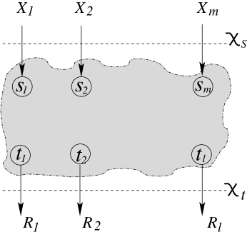
Figure 9: The source-cut and the terminal-cut of a generic sum-network

The polynomial $P(x)=(p_{1}p_{2}\ldots p_{l})x-1$, where $p_{1},p_{2},\ldots,p_{l}$ are some prime numbers, has a solution only over fields of characteristic not equal to any of $p_{1},p_{2},\ldots,p_{l}$. In Fig. 9, we show a network which, for any positive integer $n$, has a $n$-length vector linear solution over exactly those fields.

Theorem 11 (Cofinite characteristic set)

For any finite set $\mathcal{P}=\{p_{1},p_{2},\ldots,p_{l}\}$ of positive prime numbers, there exists a directed acyclic sum-network of unit-capacity edges so that for any positive integer $n$, the network is $n$-length vector linear solvable if and only if the characteristic of the alphabet field does not belong to $\mathcal{P}$.

The proof is given in Appendix C.

The polynomials considered in this subsection are very special in nature. Their solvability over a field $F$ depends only on the characteristic of $F$. Only for such a system of polynomials, it is possible to find a network which is solvably equivalent under vector linear coding of any dimension. This is because, otherwise if the polynomials have a solution over a finite extension $K$ of $F$ even though they do not have any solution over $F$, then a scalar linear solvably equivalent network has a scalar solution over $K$, but not over $F$. This implies that the network also has a vector solution over $F$ of dimension $\dim_{F}K$ even though it does not have a scalar solution over $F$.

We note that Theorems 10 and 11 are stronger than corresponding known results ([11]) for communication networks. However, by applying Construction $C_{2}$ on the sum-networks ${\cal S}_{m}$ and ${\cal S}_{m}^{\star}$, we can also get communication networks which satisfy the properties in Theorems 10 and 11 respectively.

VI Some consequences of the equivalence results

VI-A Insufficiency of linear network coding for sum-networks

It was shown in [10] that linear network coding may not be sufficient for communication networks in the sense that a rate may be achievable by non-linear coding even though the same rate may not be achievable by linear coding over any field and of any vector dimension. Such a communication network was presented in [10]. It was proved that for this network, there is a non-linear solution over the ternary alphabet $F_{3}$ even though there is no linear solution over any finite field for any vector dimension. We can get an equivalent multiple-unicast network which also satisfies the same property. Then the sum-network obtained using Construction $C_{1}$ on this multiple-unicast network satisfies the same property by Theorem 1. So for the resulting sum-network, rate $1$ is achievable over $F_{3}$ using non-linear coding but not using vector linear coding of any dimension. So, we have,

Theorem 12

There exists a sum-network with the sum defined over a finite field which is solvable by non-linear network coding, but not solvable using vector linear coding for any vector dimension.

Remark 2

It was also shown in [10] that the constructed communication network is not solvable using linear network coding over any finite commutative ring $R$ with identity, $R$-module, or by using more general forms of the linear network codes defined in [36]. The same results hold for the resulting sum-network with the additional constraint that the $R$-module needs to have the annihilator $\{0\}$ for Theorem 1(i) to hold.

VI-B Unachievability of network coding capacity of sum-networks

It is known that the network coding capacity of a communication network is independent of the alphabet ([38]). Given that the majority of the network coding literature considers zero-error recovery and noiseless link models, it is of interest to know if there always exists a code achieving the capacity exactly, unlike achieving a rate close to the capacity. In [34], a communication network (let us call it ${\cal N}_{1}$) was presented for which the network coding capacity is $1$ but there is no code of rate $\geq 1$ over any finite alphabet. We now argue that there also exists a sum-network whose network coding capacity is not achievable over any abelian group. Consider the sum-network ${\cal N}_{2}$ obtained by first taking the equivalent multiple-unicast network of ${\cal N}_{1}$, and then using Construction $C_{1}$ on it. By Theorem 1, rate $1$ is not achievable in ${\cal N}_{2}$. But it follows from Corollary 4 that the capacity of ${\cal N}_{2}$ is $1$. This gives the following theorem.

Theorem 13

There exists a sum-network whose network coding capacity is not achievable.

VII Discussion

The primary message of this paper is that sum-networks form as broad a class of networks as communication networks. Explicit construction of sum-networks from a given multiple-unicast network, and vice-versa, preserves the solvability of the networks. A sum-network and its reverse network are also shown to be linear solvably equivalent under fractional linear network coding. The solvably equivalent constructions of various types of networks from other networks enabled proving similar results, e.g., equivalence with polynomial systems, unachievability of capacity, and insufficiency of linear coding about sum-networks by using their known counterparts for communication networks. These equivalent constructions also prove the difficulty of designing network codes for sum-networks from similar results on communication networks.

VIII Acknowledgment

The authors thank Kenneth Zeger for his feedback on an earlier version of this work and particularly for pointing out other works of similar flavor. The authors would like to thank Muriel Médard for bringing [13] to their attention and pointing out a possible connection with the code-construction for the reverse network in Section IV. The authors are grateful to the Associate Editor and the anonymous referees for their constructive comments which helped improve the presentation of the paper significantly. This work was supported in part by Tata Teleservices IIT Bombay Center of Excellence in Telecomm (TICET). The work of B. K. Dey was also supported in part by a fund from the Department of Science and Technology, Government of India.

Appendix A Proof of Theorem 1

Proof of part $(i)$:  First, if the multiple-unicast network ${\cal N}_{1}$ is $n$-length vector linear solvable over $F$ then such a code can be extended to a $n$-length vector linear code of ${\cal N}_{2}$ by assigning the $n\times n$ identity matrix to all the other local coding matrices. Clearly this gives a required solution for ${\cal N}_{2}$.

Now we prove the converse. We denote the $n$-length symbol vector carried by an edge $e$ by $Y_{e}$ as in $(\ref{code4})$. By the same arguments as in the proof of Theorem 5 in page III, without loss of generality, we assume that

$$Y_{(v_{i},t_{L_{i}})}=Y_{(v_{i},t_{R_{i}})}=Y_{(u_{i},v_{i})}\mbox{ for }1\leq i\leq m,$$

$$Y_{(s_{i},t_{R_{i}})}=Y_{(s_{i},w_{i})}=X_{i}\mbox{ for }1\leq i\leq m,$$

and $$Y_{(s_{i},u_{j})}=X_{i}\text{ for }1\leq i\leq m+1,1\leq j\leq m,i\neq j.$$

Let us also assume that

$$Y_{(u_{i},v_{i})} = \mathop{\sum_{j=1}^{m+1}}_{j\neq i}\beta_{j,i}Y_{(s_{j},u_{i})}\mbox{ for }1\leq i\leq m,$$

$$Y_{(z_{i},t_{L_{i}})} = \mathop{\sum_{j=1}^{m}}\beta_{j}^{i}X_{j}\mbox{ for }1\leq i\leq m,$$

and the decoded symbols at the terminals $t_{L_{i}}$ and $t_{R_{i}}$ are respectively

$$R_{L_{i}}= \gamma_{i,L}Y_{(z_{i},t_{L_{i}})}+\gamma_{i,L}^{\prime}Y_{(v_{i},t_{L_{i}})}\mbox{ for }1\leq i\leq m,$$

and $$R_{R_{i}}= \gamma_{i,R}Y_{(s_{i},t_{R_{i}})}+\gamma_{i,R}^{\prime}Y_{(v_{i},t_{R_{i}})}\mbox{ for }1\leq i\leq m.$$

Here all the coding coefficients are $n\times n$ matrices over $F$. From $(\ref{eq:encode_klinear})$ and $(\ref{eq:decode_klinear})$, we have

$$R_{L_{i}} = \gamma_{i,L}\mathop{\sum_{j=1}^{m}}\beta_{j}^{i}X_{j}+\gamma_{i,L}^{\prime}\mathop{\sum_{j=1}^{m+1}}_{j\neq i}\beta_{j,i}X_{j}\mbox{ for }1\leq i\leq m,$$

$$R_{R_{i}} = \gamma_{i,R}X_{i}+\gamma_{i,R}^{\prime}\mathop{\sum_{j=1}^{m+1}}_{j\neq i}\beta_{j,i}X_{j}\mbox{ for }1\leq i\leq m.$$

By assumption, $R_{L_{i}}=R_{R_{i}}=\sum_{j=1}^{m+1}X_{j}$ for $1\leq i\leq m$. So $(\ref{eq:decode2_klinear})$ implies

$$\gamma_{i,L}^{\prime}\beta_{m+1,i}=I\mbox{ for }1\leq i\leq m,$$ (33a)

$$\gamma_{i,L}\beta_{i}^{i}=I\mbox{ for }1\leq i\leq m,$$ (33b)

$$\gamma_{i,L}\beta_{j}^{i}+\gamma_{i,L}^{\prime}\beta_{j,i}=I\mbox{ for }i,j=1,2,\ldots,m,j\neq i,$$

$$\gamma_{i,R}=I\mbox{ for }1\leq i\leq m,$$ (33c)

$$\gamma_{i,R}^{\prime}\beta_{j,i}=I\mbox{ for }1\leq i\leq m,1\leq j\leq m+1,j\neq i.$$

All the coding matrices in (33a), (33b), (33c) and (33) are invertible since the right hand side of the equations are the identity matrix. Eq. $(\ref{code18})$ and $(\ref{code23})$ together imply

$$\gamma_{i,L}^{\prime}=\gamma_{i,R}^{\prime}\mbox{ for }1\leq i\leq m.$$ (34)

By $(\ref{code23})$ and $(\ref{code24})$, we have

$$\gamma_{i,L}^{\prime}\beta_{j,i}=I\mbox{ for }1\leq i,j\leq m,j\neq i.$$ (35)

By $(\ref{code20})$ and $(\ref{code25})$, we have

$$\gamma_{i,L}\beta_{j}^{i}={\bf 0}\ \mbox{ for }1\leq i,j\leq m,\ j\neq i,$$

where ${\bf 0}$ denotes the all-zero $n\times n$ matrix. Since $\gamma_{i,L}$ is invertible by (33b), $\beta_{j}^{i}=0$ for $1\leq i,j\leq m,\ j\neq i$. By (33b), $\beta_{i}^{i}$ is an invertible matrix for $1\leq i\leq m$. So, we conclude that for every $i=1,\ldots,m$, $Y_{(z_{i},t_{Li})}=\beta_{i}^{i}X_{i}$. This implies that for every $i=1,\ldots,m$, $z_{i}$ can recover $X_{i}$, and thus the multiple-unicast network ${\cal N}_{1}$ is $n$-length vector linear solvable over $F$. This completes the proof of Part $(i)$.

Proof of part $(ii)$:  Now we consider the case when nodes are allowed to do non-linear network coding, i.e., nodes can send any function of the incoming symbols on an outgoing edge. For the forward part, as in part (i), a code for ${\cal N}_{1}$ can be extended to a code for ${\cal N}_{2}$.

Now we prove the “only if” part. Let us consider any network code for ${\cal N}_{2}$ over $G$. Without loss of generality, we assume

$$Y_{(s_{j},u_{i})} = X_{j}\mbox{ for }1\leq i\leq m,1\leq j\leq m+1,j\neq i,$$

$$Y_{(s_{i},w_{i})} = Y_{(s_{i},t_{R_{i}})}=X_{i}\mbox{ for }1\leq i\leq m,$$

$$Y_{(v_{i},t_{L_{i}})} = Y_{(v_{i},t_{R_{i}})}=Y_{(u_{i},v_{i})}\mbox{ for }1\leq i\leq m.$$

Further, we assume that

$$Y_{(u_{i},v_{i})} = f_{1}^{i}(X_{1},\cdots,X_{i-1},X_{i+1},\cdots,X_{m},X_{m+1})\mbox{ for }1\leq i\leq m,$$

$$Y_{(z_{i},t_{L_{i}})} = f_{2}^{i}(X_{1},\cdots,X_{i-1},X_{i},X_{i+1},\cdots,X_{m})\mbox{ for }1\leq i\leq m,$$

and the decoded symbols at the terminals are

$$R_{R_{i}} = g_{1}^{i}(Y_{(v_{i},t_{R_{i}})},Y_{(s_{i},t_{R_{i}})}),$$ (37a)

$$R_{L_{i}} = g_{2}^{i}(Y_{(v_{i},t_{L_{i}})},Y_{(z_{i},t_{L_{i}})}).$$ (37b)

Here all the symbols carried by the links are symbols from $G$.

We need to show that for every $i=1,2,\ldots,m$, communicating the sum of the source symbols to the terminals $t_{L_{i}}$ and $t_{R_{i}}$ is possible only if $f_{2}^{i}$ is an $1-1$ function only of the symbol $X_{i}$ and is independent of the other variables.

By $(\ref{eq:nonlinear_decode})$, for every $i=1,2,\ldots,m$, the functions $f_{1}^{i}$, $f_{2}^{i}$, $g_{1}^{i}$ and $g_{2}^{i}$ must satisfy the following conditions.

$$g_{1}^{i}(f_{1}^{i},X_{i}) = X_{1}+\cdots+X_{i-1}+X_{i}+X_{i+1}+\cdots+X_{m}+X_{m+1},$$ (38a)

$$g_{2}^{i}(f_{1}^{i},f_{2}^{i}) = X_{1}+\cdots+X_{i-1}+X_{i}+X_{i+1}+\cdots+X_{m}+X_{m+1}.$$ (38b)

Now we prove the following claims for the functions $g_{1}^{i},g_{2}^{i},f_{1}^{i},f_{2}^{i}$ for $1\leq i\leq m$.

Claim 1

For every $i=1,2,\ldots,m$, $f_{1}^{i}$ is bijective on each variable $X_{j},\mbox{ for }1\leq j\leq m+1,j\neq i$, for any fixed values of the other variables.

Proof:  Let us consider any $j\neq i$. For any fixed values of $\{X_{k}|k\neq j\}$, $(\ref{nonlinear_code9})$ implies that $g_{1}^{i}(f_{1}^{i}(\cdot,X_{j},\cdot),\cdot)$ is a bijective function of $X_{j}$. This in turn implies that $f_{1}^{i}$ is a bijective function of $X_{j}$ for any fixed values of the other variables.

Claim 2

For every $i=1,2,\ldots,m$, $g_{1}^{i}(\cdot,\cdot)$ is bijective on each argument for any fixed value of the other argument.

Proof:  For any element of $G$, by claim 1, there exists a set of values for $\{X_{j}|j\neq i\}$ so that the first argument $f_{1}^{i}(\cdot)$ of $g_{1}^{i}$ takes that value. For such a set of fixed values of $\{X_{j}|j\neq i\}$, $g_{1}^{i}(\cdot,X_{i})$ is a bijective function of $X_{i}$ by (38a). Now, consider any $j\neq i$ and fix some values for $\{X_{k}|k\neq j\}$. Again by (38a), $g_{1}^{i}(f_{1}^{i}(\cdot,X_{j},\cdot),\cdot)$ is a bijective function of $X_{j}$. This implies that $g_{1}^{i}$ is a bijective function of its first argument for any fixed value of the second argument.

Claim 3

For every $i=1,2,\ldots,m$, $f_{1}^{i}$ is symmetric, i.e., interchanging the values of any two variables in its arguments does not change the value of $f_{1}^{i}$.

Proof:  For some fixed values of all the arguments of $f_{1}^{i}$, suppose the value of $f_{1}^{i}$ is $c_{1}$. We also fix the value of $X_{i}$ as $c_{2}$. Suppose $g_{1}^{i}(c_{1},c_{2})=c_{3}$. Now we interchange the values of the variables $X_{j}$ and $X_{k}$ where $j\neq i\neq k$. Then it follows from Claim 2 and (38a) that the value of $f_{1}^{i}$ must remain the same.

Claim 4

For every $i=1,2,\ldots,m$, $f_{2}^{i}$ is a bijective function of $X_{i}$ for any fixed values of $\{X_{j}|j=1,2,\ldots,m,j\neq i\}$.

Proof:  For any fixed values of $\{X_{j}|j=1,2,\ldots,m,j\neq i\}$ and $X_{m+1}$, $g_{2}^{i}(\cdot,f_{2}^{i}(\cdot,X_{i},\cdot))$ is a bijective function of $X_{i}$ by equation $(\ref{nonlinear_code8})$. This implies that $f_{2}^{i}$ is a bijective function of $X_{i}$ for any fixed values of the other arguments.

Claim 5

For every $i=1,2,\ldots,m$, $g_{2}^{i}(\cdot,\cdot)$ is bijective on each argument for any fixed value of the other argument.

Proof:  By equation (38b), $g_{2}^{i}(f_{1}^{i}(\cdot,X_{m+1}),f_{2}^{i}(\cdot))$ and $g_{2}^{i}(f_{1}^{i}(\cdot),f_{2}^{i}(\cdot,X_{i},\cdot))$ are both bijective functions of $X_{m+1}$ and $X_{i}$ respectively for any fixed values of the omitted variables. This implies that $g_{2}^{i}$ is a bijective function of the first and the second argument for the other argument fixed.

Now to prove that for every $i=1,2,\ldots,m$, the value of $f_{2}^{i}(X_{1},\cdots,X_{m})$ does not depend on $\{X_{j}|j=1,\ldots,m;j\neq i\}$, it is sufficient to prove that for any set of fixed values $X_{1}=a_{1},\ldots,X_{m}=a_{m}$, changing the value of $X_{j}$ ($j\neq i$) to any $b_{j}\in G$ does not change the value of $f_{2}^{i}$. Let us assign $X_{m+1}=b_{j}$. By (38b), the value of $g_{2}^{i}$ does not change by interchanging the values of $X_{j}$ and $X_{m+1}$. Also, the value of $f_{1}^{i}$ does not change by this interchange by Claim 3. So, by Claim 5, the value of $f_{2}^{i}$ also does not change by this change of value of $X_{j}$ from $a_{j}$ to $b_{j}$.

Now using Claim 4, it follows that $f_{2}^{i}$ is a bijective function of only the variable $X_{i}$. This completes the proof of part (ii) of the theorem. It is interesting to note that a somewhat similar technique was independently used in [19] to prove that there is no non-linear solution for the network ${\cal S}_{3}$ (Fig. 7).

Proof of part $(iii)$:  In the same way as in the proof of part (i), a $n$-length vector linear code of ${\cal N}_{1}^{\prime}$ can be extended to a $n$-length vector linear code of ${\cal N}_{2}^{\prime}$. Now we prove the “only if” part. Let us consider a $n$-length vector linear code of ${\cal N}_{2}^{\prime}$. We assume that for every $i=1,2,\ldots,m$, the edge $(w_{i},s_{i})$ carries a linear combination

$$Y_{(w_{i},s_{i})}=\mathop{\sum_{j=1}^{m}}\beta_{i,j}X_{L_{j}},$$

where $\beta_{i,j}\in F^{n\times n}$.

Without loss of generality, we assume that

$$Y_{(u_{j},s_{i})}= Y_{(v_{j},u_{j})}\mbox{ for }1\leq j\leq m,1\leq i\leq m+1,j\neq i,$$

$$Y_{(t_{L_{j}},v_{j})}= Y_{(t_{L_{j}},z_{j})}=X_{L_{j}}\mbox{ for }1\leq j\leq m,$$

and $$Y_{(t_{R_{j}},s_{j})}= Y_{(t_{R_{j}},v_{j})}=X_{R_{j}}\mbox{ for }1\leq j\leq m.$$

We further assume that

$$Y_{(v_{j},u_{j})} = \beta_{L,j}Y_{(t_{L_{j}},v_{j})}+\beta_{R,j}Y_{(t_{R_{j}},v_{j})}\mbox{ for }1\leq j\leq m.$$ (39a)

and that for $1\leq i\leq m+1$, the decoded symbols $R_{i}$ at the terminals $s_{i}$ are

$$R_{i} = \mathop{\sum_{j=1}^{m}}_{j\neq i}\gamma_{j,i}Y_{(u_{j},s_{i})}+\gamma_{i,i}Y_{(t_{R_{i}},s_{i})}+\gamma_{i}Y_{(w_{i},s_{i})}1\leq i\leq m,$$

$$\text{ and }R_{m+1} = \mathop{\sum_{j=1}^{m}}\gamma_{j,m+1}Y_{(u_{j},s_{m+1})}.$$ (40a)

Here all the coding coefficients and decoding coefficients are $n\times n$ matrices over $F$, and the message vectors $Y_{(.,.)}$ carried by the links are $n$-length vectors over $F$.

By $(\ref{eq:reverse_code})$ and $(\ref{eq:reverse_decode})$, we have

$$R_{i} = \mathop{\sum_{j=1}^{m}}_{j\neq i}\gamma_{j,i}(\beta_{L,j}X_{L_{j}}+\beta_{R,j}X_{R_{j}})+\gamma_{i,i}X_{R_{i}}+\gamma_{i}\mathop{\sum_{j=1}^{m}}\beta_{i,j}X_{L_{j}}\mbox{ for }1\leq i\leq m,$$ (41a)

$$\mbox{and }R_{m+1} = \mathop{\sum_{j=1}^{m}}\gamma_{j,m+1}(\beta_{L,j}X_{L_{j}}+\beta_{R,j}X_{R_{j}}).$$ (41b)

By assumption, for every $i=1,2,\ldots,m+1$,

$$R_{i}=\sum_{j=1}^{m}(X_{L_{j}}+X_{R_{j}}).$$ (42)

By (41) and (42), we have

$$\gamma_{i,i}=I\mbox{ for }1\leq i\leq m,$$ (43a)

$$\gamma_{j,m+1}\beta_{L,j}=\gamma_{j,m+1}\beta_{R,j}=I\mbox{ for }1\leq j\leq m,$$ (43b)

$$\gamma_{j,i}\beta_{R,j}=I\mbox{ for }1\leq i,j\leq m,j\neq i,$$ (43c)

$$\gamma_{j,i}\beta_{L,j}+\gamma_{i}\beta_{i,j}=I\mbox{ for }1\leq i,j\leq m,j\neq i,$$ (43d)

$$\gamma_{i}\beta_{i,i}=I\mbox{ for }1\leq i\leq m.$$ (43e)

All the coding matrices in (43a), (43b), (43c) and (43e) are invertible since the right hand side of the equations are the identity matrix. Equation (43b) implies that $\beta_{L,j}=\beta_{R,j}$ for $1\leq j\leq m$. By this, (43c) implies $\gamma_{j,i}\beta_{L,j}=I$. Then (43d) implies

$$\gamma_{i}\beta_{i,j}={\bf 0}\ \mbox{ for }1\leq i,j\leq m,j\neq i,$$

where ${\bf 0}$ is the $n\times n$ all-zeros matrix.

Since $\gamma_{i}$ is an invertible matrix for $1\leq i\leq m$ by (43e), we have

$$\beta_{i,j}={\bf 0}\ \mbox{ for }1\leq i,j\leq m,j\neq i.$$

Also from (43e), $\beta_{i,i}$ is invertible. So, for every $i=1,2,\ldots,m$, the edge $(w_{i},s_{i})$ carries a nonzero scalar multiple of $X_{L_{i}}$, which implies that the reverse multiple-unicast network ${\cal N}_{1}^{\prime}$ is solvable over $F$. This completes the proof of part (iii).

Proof of part $(iv)$: First, similar to part (iii), any code over $G$ for ${\cal N}_{1}^{\prime}$ can be extended to a code over $G$ for ${\cal N}_{2}^{\prime}$.

Now we prove the converse. Consider any network code over $G$ for ${\cal N}_{2}^{\prime}$ where the terminal $s_{i}$ computes

$$R_{i}=\sum_{i=1}^{m}(X_{L_{i}}+X_{R_{i}})\hskip 5.69054pt\mbox{for }i=1,2,\ldots,m+1.$$

Without loss of generality, we assume that

$$Y_{(u_{i},s_{j})}=Y_{(v_{i},u_{i})}\mbox{ for }1\leq i\leq m,\,\,\,1\leq j\leq m+1,i\neq j.$$

$$Y_{(t_{R_{i}},v_{i})}=Y_{(t_{R_{i}},s_{i})}=X_{R_{i}}\mbox{ for }1\leq i\leq m,$$

$$Y_{(t_{L_{i}},z_{i})}=Y_{(t_{L_{i}},v_{i})}=X_{L_{i}}\mbox{ for }1\leq i\leq m,$$

We further assume that

$$Y_{(v_{i},u_{i})} = f_{i}(X_{L_{i}},X_{R_{i}})\mbox{ for }1\leq i\leq m,$$

$$Y_{(w_{i},s_{i})} = f_{i}^{\prime}(X_{L_{1}},X_{L_{2}},\cdots,X_{L_{m}}),\mbox{ for }1\leq i\leq m,$$

and the decoded symbols are

$$R_{i} =g_{i}(Y_{(w_{i},s_{i})},Y_{(u_{1},s_{i})},\cdots,Y_{(u_{i-1},s_{i})},Y_{(u_{i+1},s_{i})},\cdots,Y_{(u_{m},s_{i})},Y_{(t_{R_{i}},s_{i})})$$ (45a)

for $$1\leq i\leq m$$; and

$$R_{m+1} =g_{m+1}(Y_{(u_{1},s_{m+1})},\cdots,Y_{(u_{m},s_{m+1}))}.$$ (45b)

Now we state some claims which can be proved using similar arguments as in the proof of part (ii) of the theorem. We omit the proof of these claims.

1. As a function of the variables $X_{L_{i}},X_{R_{i}}$; $i=1,2,\ldots,m$, $g_{m+1}$ is bijective in each variable for fixed values of the other variables.

2. The function $g_{m+1}$ is bijective in each variable $Y_{(u_{i},s_{m+1})}$ for fixed values of the other variables.

3. For $i=1,2,\ldots,m$, $f_{i}(X_{L_{i}},X_{R_{i}})$ is a bijective function of each variable for a fixed value of the other variable.

4. For $i=1,2,\ldots,m$, $f_{i}(X_{L_{i}},X_{R_{i}})$ is symmetric on its arguments.

5. For $i=1,2,\ldots,m$, $g_{i}$ is bijective on each of its arguments for fixed values of the other arguments.

First by (45a), $g_{i}(f_{i}^{\prime}(\cdot,X_{i},\cdot),\cdots)$, and thus $f_{i}^{\prime}(\cdot,X_{i},\cdot)$, is a bijective function of $X_{i}$ for any fixed values of the other variables. Now we prove that $f_{i}^{\prime}$ is a function of only $X_{L_{i}}$, and it is independent of the other variables. Fix a $k\neq i$. It is sufficient to prove that for any fixed values of $X_{L_{j}},j=1,2,\ldots,m,j\neq k$, the value of $f_{i}^{\prime}$ does not change if the value of $X_{L_{k}}$ is changed from, say, $a$ to $b$. Let us fix $X_{L_{k}}=a$. Let us further fix $X_{R_{k}}=b$ and the variables $X_{R_{j}}$ for $j\neq k$ to arbitrary values. Now, by interchanging the values of $X_{L_{k}}$ and $X_{R_{k}}$, the value of $g_{i}$ does not change, since the sum of the variables does not change. Further, all the arguments of $g_{i}$ other than $f_{i}^{\prime}$ does not change since $f_{k}$ is symmetric on its arguments. So by claim 5, the value of $f_{i}^{\prime}$ also does not change by this interchange. But this means that the value of $f_{i}^{\prime}$ does not change by the change of the value of $X_{L_{k}}$ from $a$ to $b$. This completes the proof of part (iv).

Appendix B Proof of Theorem 10

Define $m=p_{1}p_{2}\ldots p_{l}+2$, where the empty product is defined to be $1$. We prove that the network ${\cal S}_{m}$ satisfies the condition in the theorem. First we prove that if, for any $n$, it is possible to communicate the sum of the sources by $n$-length vector linear network coding over a field $F$ to all the terminals in ${\cal S}_{m}$, then the characteristic of $F$ must be from $\mathcal{P}$. For $i=1,2,\ldots,m$, the message vector generated by the source $s_{i}$ is denoted by $X_{i}\in F^{n}$.

Without loss of generality, we assume that

$$Y_{(s_{i},t_{j})} = X_{i}\mbox{ for }1\leq i,j\leq m-1,i\neq j,$$

$$Y_{(s_{i},u_{i})} = X_{i},\mbox{ for }1\leq i\leq m-1,$$

$$Y_{(s_{m},u_{i})} = X_{m}\mbox{ for }1\leq i\leq m-1,$$

$$\text{and }Y_{(v_{i},t_{i})} = Y_{(v_{i},t_{m})}=Y_{(u_{i},v_{i})}\mbox{ for }1\leq i\leq m-1.$$

Let us further assume that

$$Y_{(u_{i},v_{i})} = \beta_{i,1}Y_{(s_{i},u_{i})}+\beta_{i,2}Y_{(s_{m},u_{i})}\mbox{ for }1\leq i\leq m-1$$ (46a)

and the vectors computed at the terminals are

$$R_{i} = \mathop{\sum_{j=1}^{m-1}}_{j\neq i}\gamma_{j,i}Y_{(s_{j},t_{i})}+\gamma_{i,i}Y_{(v_{i},t_{i})}\mbox{ for }1\leq i\leq m-1,$$ (47a)

$$\text{ and }R_{m} = \sum_{j=1}^{m-1}\gamma_{j,m}Y_{(v_{j},t_{m})}.$$ (47b)

Here all the coding and decoding coefficients $\beta_{i,j},\gamma_{i,j}$ are $n\times n$ matrices over $F$, and the message vectors $X_{i}$ and the messages $Y_{(.,.)}$ carried by the links are length-$n$ vectors over $F$.

By assumption, each terminal decodes the sum of all the sources. That is,

$$R_{i}=\sum_{j=1}^{m}X_{j}\mbox{ for }i=1,2,\ldots,m.$$ (48)

From (46) and (47), we have

$$R_{i}= \mathop{\sum_{j=1}^{m-1}}_{j\neq i}\gamma_{j,i}X_{j}+\gamma_{i,i}\beta_{i,1}X_{i}+\gamma_{i,i}\beta_{i,2}X_{m}\,\,\text{ for }i=1,2,\ldots,m-1$$ (49)

and

$$R_{m}=\sum_{j=1}^{m-1}\gamma_{j,m}\beta_{j,1}X_{j}+\left(\sum_{j=1}^{m-1}\gamma_{j,m}\beta_{j,2}\right)X_{m}.$$ (50)

Since (48) is true for all values of $X_{1},X_{2},\ldots,X_{m}\in F^{n}$, (49) and (50) imply

$$\gamma_{j,i}=I\mbox{ for }1\leq i,j\leq m-1,i\neq j,$$ (51)

$$\gamma_{i,i}\beta_{i,1}=I\mbox{ for }1\leq i\leq m-1,$$ (52)

$$\gamma_{i,i}\beta_{i,2}=I\mbox{ for }1\leq i\leq m-1,$$ (53)

$$\gamma_{i,m}\beta_{i,1}=I\mbox{ for }1\leq i\leq m-1,$$ (54)

$$\sum_{i=1}^{m-1}\gamma_{i,m}\beta_{i,2}=I,$$ (55)

where $I$ denotes the $n\times n$ identity matrix over $F$. All the coding matrices in (51)–(54) are invertible since the right hand side of the equations are the identity matrix. Equations (52) and (53) imply $\beta_{i,1}=\beta_{i,2}$ for $1\leq i\leq m-1$. So, (55) gives

$$\sum_{i=1}^{m-1}\gamma_{i,m}\beta_{i,1}=I.$$

Now, using (54), we get

$$\sum_{i=1}^{m-1}I=I,$$

$$\Rightarrow (m-1)I=I,$$

$$\Rightarrow (m-2)I={\bf 0}.$$

This is true if and only if the characteristic of $F$ divides $m-2$. So, the sum of the sources can be communicated in ${\cal S}_{m}$ by vector linear network coding only if the characteristic of $F$ belongs to $\mathcal{P}$.

Now, if the characteristic of $F$ belongs to $\mathcal{P}$, then for any block length $n$, in particular for scalar network coding for $n=1$, every coding matrix in (46a) and (47) can be chosen to be the identity matrix. The terminals then recover the sum of the sources. This completes the proof.

Appendix C Proof of Theorem 11

Consider the network ${\cal S}_{m}^{*}$ shown in Fig. 9 for $m=p_{1}p_{2}\ldots p_{l}+2$. We will show that this network satisfies the condition of the theorem. We first prove that if it is possible to communicate the sum of the source messages using vector linear network coding over a field $F$ to all the terminals in ${\cal S}_{m}^{*}$, then the characteristic of $F$ must not divide $m-2$. For $i=1,2,\ldots,m$, let the message vector generated by the source $s_{i}$ be denoted by $X_{i}\in F^{n}$. Each terminal $t_{i}$ computes a linear combination $R_{i}$ of the received vectors.

Without loss of generality, let us assume that

$$Y_{(s_{i},t_{i})} = X_{i}\mbox{ for }1\leq i\leq m-1,$$ (56a)

$$Y_{(s_{i},u_{j})} = X_{i}\mbox{ for }1\leq i,j\leq m-1,i\neq j,$$ (56b)

$$\text{ and }Y_{(v_{i},t_{i})} = Y_{(v_{i},t_{m})}=Y_{(u_{i},v_{i})}\mbox{ for }1\leq i\leq m-1.$$ (56c)

Further, suppose

$$Y_{(u_{i},v_{i})} = \mathop{\sum_{j=1}^{m-1}}_{j\neq i}\beta_{j,i}Y_{(s_{j},u_{i})}\mbox{ for }1\leq i\leq m-1,$$ (56d)

$$R_{i} = \gamma_{i,1}Y_{(s_{i},t_{i})}+\gamma_{i,2}Y_{(v_{i},t_{i})}\mbox{ for }1\leq i\leq m-1,$$ (57a)

$$\text{and }R_{m} = \sum_{j=1}^{m-1}\gamma_{j,m}Y_{(v_{j},t_{m})}.$$ (57b)

Here all the coding coefficients $\beta_{i,j},\gamma_{i,j}$ are $n\times n$ matrices over $F$.

By assumption, each terminal decodes the sum of all the source messages. That is,

$$R_{i}=\sum_{j=1}^{m-1}X_{j}\mbox{ for }i=1,2,\ldots,m.$$ (58)

From (56) and (57), we have

$$R_{i} = \mathop{\sum_{j=1}^{m-1}}_{j\neq i}\gamma_{i,2}\beta_{j,i}X_{j}+\gamma_{i,1}X_{i}\mbox{ for }i=1,2,\ldots,m-1,$$ (59)

$$\text{and }R_{m} = \sum_{i=1}^{m-1}\gamma_{i,m}\left(\mathop{\sum_{j=1}^{m-1}}_{j\neq i}\beta_{j,i}X_{j}\right)$$ (60)

$$= \sum_{j=1}^{m-1}\left(\mathop{\sum_{i=1}^{m-1}}_{i\neq j}\gamma_{i,m}\beta_{j,i}\right)X_{j}.$$

Since (58) is true for all values of $X_{1},X_{2},\ldots,X_{m}\in F^{n}$, (59) and (60) imply

$$\gamma_{i,2}\beta_{j,i}=I\mbox{ for }1\leq i,j\leq m-1,i\neq j,$$ (61)

$$\gamma_{i,1}=I\mbox{ for }1\leq i\leq m-1,$$ (62)

$$\mathop{\sum_{i=1}^{m-1}}_{i\neq j}\gamma_{i,m}\beta_{j,i}=I\mbox{ for }1\leq j\leq m-1.$$ (63)

All the coding matrices in (61), (62) are invertible since the right hand side of the equations are the identity matrix. Equation (61) implies $\beta_{j,i}=\beta_{k,i}$ for $1\leq i,j,k\leq m-1$, $j\neq i\neq k$. So, let us denote all the equal co-efficients $\beta_{j,i};1\leq j\leq m-1,j\neq i$ by $\beta_{i}$. Then (63) can be rewritten as

$$\mathop{\sum_{i=1}^{m-1}}_{i\neq j}\gamma_{i,m}\beta_{i}=I\mbox{ for }1\leq j\leq m-1.$$ (64)

Equating the left hand side of (64) for two values of $j$ (say, $j$ and $k$), we have

$$\gamma_{j,m}\beta_{j}=\gamma_{k,m}\beta_{k}\mbox{ for }1\leq j,k\leq m-1.$$

Then (64) gives

$$(m-2)\gamma_{1,m}\beta_{1}=I.$$ (65)

Equation (65) implies that $(m-2)$ is invertible in $F$, that is, the characteristic of $F$ does not devide $(m-2)$. So the sum of the source messages can be communicated in ${\cal S}_{m}^{*}$ by $n$-length vector linear network coding over $F_{q}$ only if the characteristic of $F$ does not divide $(m-2)$.

Now, if the characteristic of $F$ does not divide $(m-2)$, then for any block length $n$, every coding matrix in (56d) and (57a) can be chosen to be the identity matrix, and $\gamma_{j,m}=(m-2)^{-1}I$ in (57b). The terminals $t_{1},t_{2},\cdots,t_{m}$ then recover the sum of the source messages. This completes the proof.

Brijesh Kumar Rai (S’09-M’11) received the B.E. degree in Electronics and Communication Engineering from F.E.T., R.B.S College, Bichpuri, Agra, India, in 2001, the M.Tech. degree in Electrical Engineering from Indian Institute of Technology Kanpur, Kanpur, India, in 2004, and the Ph.D. degree in Electrical Engineering from Indian Institute of Technology Bombay, Mumbai, India, in 2010. Currently, he is an Assistant Professor at the Department of Electronics and Electrical Engineering, Indian Institute of Technology Guwahati, Guwahati, India. From September 2010 to May 2011, he was a Postdoctoral Fellow at Network and Computer Science Department - INFRES, Télécom ParisTech, Paris, France. His research interests include information theory, communications, coding theory and network coding. Prof. Rai has been selected for Microsoft Young Outstanding Faculty Award 2011-2012 at the Department of Electronics and Electrical Engineering, Indian Institute of Technology Guwahati, Guwahati, India.

Bikash Kumar Dey (S’00-M’04) received his B.E. degree in Electronics and Telecommunication Engineering from Bengal Engineering College, Howrah, India, in 1996. He received his M.E. degree in Signal Processing and Ph.D. in Electrical Communication Engineering from the Indian Institute of Science in 1999 and 2003 respectively. From August 1996 to June 1997, he worked at Wipro Infotech Global R&D. In February 2003, he joined Hellosoft India Pvt. Ltd. as a Technical Member. In June 2003, he joined the International Institute of Information Technology, Hyderabad, India, as Assistant Professor. In May 2005, he joined the Department of Electrical Engineering of Indian Institute of Technology Bombay where he works as Associate Professor. His research interests include information theory, coding theory, and network coding. He was awarded the Prof. I.S.N. Murthy Medal from IISc as the best M.E. student in the Department of Electrical Communication Engineering and Electrical Engineering for 1998-1999 and Alumni Medal for the best Ph.D. thesis in the Division of Electrical Sciences for 2003-2004.

References

- [1] R. Ahlswede, N. Cai, S.-Y. R. Li, and R. W. Yeung, “Network information flow,” IEEE Trans. Inform. Theory, vol. 46, no. 4, pp. 1204–1216, 2000.
- [2] S.-Y. R. Li, R. W. Yeung, and N. Cai, “Linear network coding,” IEEE Trans. Inform. Theory, vol. 49, no. 2, pp. 371–381, 2003.
- [3] R. Koetter and M. Médard, “An algebraic approach to network coding,” IEEE/ACM Transactions on Networking, vol. 11, no. 5, pp. 782–795, 2003.
- [4] S. Jaggi, P. Sanders, P. A. Chou, M. Effros, S. Egner, K. Jain, and L. Tolhuizen, “Polynomial time algorithms for multicast network code construction,” IEEE Trans. Inform. Theory, vol. 51, no. 6, pp. 1973–1982, 2005.
- [5] T. Ho, R. Koetter, M. Médard, M. Effros, J. Shi, and D. Karger, “A random linear network coding approach to multicast,” IEEE Trans. Inform. Theory, vol. 52, no. 10, pp. 4413–4430, 2006.
- [6] A. R. Lehman and E. Lehman, “Complexity classification of network information flow problems,” in Proceedings of 41st Annual Allerton Conference on Communication, Control, and Computing, Monticello, IL, October 2003.
- [7] M. Langberg and A. Sprintson, “On the hardness of approximating the network coding capacity,” in Proc. ISIT, (Toronto, Canada), 2008.
- [8] M. Médard, M. Effros, T. Ho, and D. Karger, “On coding for nonmulticast networks,” in Proceedings of 41st Annual Allerton Conference on Communication, Control, and Computing, Monticello, IL, October 2003.
- [9] S. Riis, “Linear versus nonlinear boolean functions in network flow,” in Proceedings of 38th Annual Conference on Information Sciences and Systems, Princeton, NJ, March 2004.
- [10] R. Dougherty, C. Freiling, and K. Zeger, “Insufficiency of linear coding in network information flow,” IEEE Trans. Inform. Theory, vol. 51, no. 8, pp. 2745–2759, 2005.
- [11] R. Dougherty, C. Freiling, and K. Zeger, “Linear network codes and systems of polynomial equations,” IEEE Trans. Inform. Theory, vol. 54, no. 5, pp. 2303–2316, 2008.
- [12] R. Dougherty and K. Zeger, “Nonreversibility and equivalent constructions of multiple-unicast networks,” IEEE Trans. Inform. Theory, vol. 52, no. 11, pp. 5067–5077, 2006.
- [13] R. Koetter, M. Effros, T. Ho, and M. Médard, “Network codes as codes on graphs,” in Proc. CISS, 2004.
- [14] S. Riis, “Reversible and irreversible information networks,” IEEE Trans. Inform. Theory, vol. 53, no. 11, pp. 4339–4349, 2007.
- [15] J. Korner and K. Marton, “How to encode the modulo-two sum of binary sources,” IEEE Trans. Inform. Theory, vol. 25, no. 2, pp. 219–221, 1979.
- [16] D. Krithivasan and S. S. Pradhan, “An achievable rate region for distributed source coding with reconstruction of an arbitrary function of the sources,” in Proc. ISIT, (Toronto, Canada), 2008.
- [17] R. G. Gallager, “Finding parity in a simple broadcast network,” IEEE Trans. Inform. Theory, vol. 34, pp. 176–180, 1988.
- [18] A. Ramamoorthy, “Communicating the sum of sources over a network,” in Proc. ISIT, (Toronto, Canada), pp. 1646–1650, 2008.
- [19] M. Langberg and A. Ramamoorthy, “Communicating the sum of sources in a 3-sources/3-terminals network,” in Proc. ISIT, (Seoul, Korea), 2009.
- [20] R. Appuswamy, M. Franceschetti, N. Karamchandani, and K. Zeger, “Network computing capacity for the reverse butterfly network,” in Proc. ISIT, (Seoul, Korea), 2009.
- [21] R. Appuswamy, M. Franceschetti, N. Karamchandani, and K. Zeger, “Network coding for computing,” in Proceedings of Annual Allerton Conference, (UIUC, IIlinois, USA), 2008.
- [22] M. Langberg and A. Ramamoorthy, “Communicating the sum of sources in a 3-sources/3-terminals network; revisited,” in Proc. ISIT, 2010.
- [23] A. Ramamoorthy and M. Langberg, “Communicating the sum of sources over a network,” available at http://arxiv.org/abs/1001.5319, 2010.
- [24] S. Shenvi and B. K. Dey, “A necessary and sufficient condition for solvability of a 3s/3t sum-network,” in Proc. ISIT, (Austin, Texas, USA), June 2010.
- [25] S. Shenvi and B. K. Dey, “On the solvability of 3-source 3-terminal sum-networks,” available at http://arxiv.org/abs/1001.4137.
- [26] R. Appuswamy, M. Franceschetti, N. Karamchandani, and K. Zeger, “Network coding for computing part I : Cut-set bounds,” available at http://arxiv.org/abs/0912.2820.
- [27] T. S. Han and K. Kobayashi, “A dichotomy of functions of correlated sources ,” IEEE Trans. Inform. Theory, vol. 33, no. 1, pp. 69–86, 1987.
- [28] A. Orlitsky and J. R. Roche, “Coding for computing,” IEEE Trans. Inform. Theory, vol. 47, no. 3, pp. 903–917, 2001.
- [29] H. Feng, M. Effros, and S. A. Savari, “Functional source coding for networks with receiver side information,” in Proceedings of the Allerton Conference on Communication, Control, and Computing, September 2004.
- [30] J. N. Tsistsiklis, “Decentralized detection by a large number of sensors,” Mathematics of Control, Signals and Systems, vol. 1, no. 2, pp. 167–182, 1988.
- [31] A. Giridhar and P. R. Kumar, “Computing and communicating functions over sensor networks,” IEEE J. Select. Areas Commun., vol. 23, no. 4, pp. 755–764, 2005.
- [32] Y. Kanoria and D. Manjunath, “On distributed computation in noisy random planar networks,” in Proceedings of ISIT, Nice, France, 2008.
- [33] S. Boyd, A. Ghosh, B. Prabhaar, and D. Shah, “Gossip algorithms: design, analysis and applications,” in Proceedings of IEEE INFOCOM, (Miami, USA), 2005.
- [34] R. Dougherty, C. Freiling, and K. Zeger, “Unachievability of network coding capacity,” IEEE Trans. Inform. Theory, vol. 52, no. 6, pp. 2365–2372, 2006.
- [35] M. F. Atiyah and I. G. MacDonald, Introduction to Commutative Algebra. Reading, Mass.-London-Don Mills, Ont.: Addison-Wesley Publishing Company, 1969.
- [36] S. Jaggi, M. Effros, T. Ho, and M. Médard, “On linear network coding,” in Proceedings of 42st annual allerton conference on communication, control, and computing, (UIUC, Illinois, USA), October 2006.
- [37] A. Ramamoorthy and M. Langberg 2008. personal communication.
- [38] J. Cannons, R. Dougherty, C. Freiling, and K. Zeger, “Network routing capacity,” IEEE Trans. Inform. Theory, vol. 52, no. 3, pp. 777–788, 2006.