The Binary History and the Magnetic Field of Neutron Stars

Abstract

There has been strong observational evidence suggesting a causal connection between the binary history of neutron stars and the evolution of their magnetic field. In this article we discuss one of the plausible mechanisms proposed for the evolution of the surface magnetic field, that of the diamagnetic screening of the field by accreted material.

1 Introduction

Radio pulsar observations have established that neutron stars associated with binaries have magnetic fields significantly smaller than in isolated neutron stars which have field strengths clustered around $10^{12}$ G (excluding magnetars). It is understood that processing in binaries alter the magnetic field strength of neutron stars giving rise to the low-field binary and millisecond pulsars. Unfortunately, till date there is no clear consensus regarding either the nature of the internal configuration or the time evolution of the magnetic field in neutron stars. Depending on the generation mechanism the field could either be supported by the crustal currents or by the Abrikosov fluxoids of the proton superconductor in the stellar core.

Accordingly, two classes of models have been proposed for the evolution of the magnetic field in accreting neutron stars - one relating the magnetic field evolution to the spin evolution of the star assuming the field to be contained in the superconducting fluxoids and the other attributing the field evolution to direct effects of mass accretion on the crustal currents. In an accretion heated crust, the decay takes place principally as a result of rapid dissipation of currents due to the decrease in the electrical conductivity and hence a reduction in the ohmic dissipation time scale. Interestingly, the mechanism of ohmic decay, unique to the crustal currents, is also used in models where spin-down is invoked for flux expulsion, for a subsequent dissipation of such flux in the crust. Therefore, the theoretical efforts in modeling the plausible mechanisms have so far been concentrated on the ohmic dissipation of currents in the outer crust (Konar & Bhattacharya 2001; Bhattacharya 2002).

Another possible mechanism is to screen the surface field by the accreting material. As the highly conducting accreting plasma flows horizontally from the polar caps to lower latitudes, the magnetic field lines are dragged along with it, by virtue of flux freezing. This dragging may lead to the creation of additional horizontal components at the expense of vertical ones producing an effective screening of the dipolar surface field. Interestingly, this mechanism would not depend on the location of the field in the stellar interior and would be effective irrespective of the nature of the interior currents. Even though this was suggested quite early on (Bisnovatyi-Kogan & Komberg 1974; Blandford, De Campli & Königl 1979; Taam & van den Heuvel 1986; Romani 1990, 1995), it is only recently that the problem is being investigated in quantitative detail. One-dimensional plane-parallel modeling by Cumming, Zweibel & Bildsten (2001) indicates that the diamagnetic screening is ineffective for field strengths above $\sim 10^{10}$G and for accretion rates below $\sim$ 1 % of the local Eddington rate. Recently, Melatos & Phinney (2001) have calculated the hydromagnetic structure of a neutron star accreting symmetrically at both magnetic poles as a function of the accreted mass. According to their calculation the magnetic dipole moment scales as $B_{0}^{1.3}\mbox{$\dot{M}$}^{0.18}M_{a}^{\-1.3}$ where $B_{0}$, $\dot{M}$ and $M_{a}$ are the initial field strength, the rate of accretion and the total accreted mass.

2 Material Flow : 2-Dimensional Model

Figure 1: Flow velocity (marked $a$), $\rho{\bf v}$, and its divergence (marked $b$) in a right-angular slice ($0\leq\theta\leq\pi/2$, $0.25\leq r\leq 1.0$) with $r_{m}=0.75$, $r_{b}=0.5$. The panels marked $1,2$ correspond to $c=0.0,1.0$.

In a recent work we have proposed a 2-dimensional flow pattern of the accreted material to demonstrate the mechanism of diamagnetic screening (Choudhuri & Konar 2002). The accreted material, confined to the poles by strong magnetic stresses, accumulates in a column and sinks below the surface when the pressure of the accretion column exceeds the magnetic pressure. From the bottom of the accretion column, the material from both the poles move to the lower latitudes in an equator-ward flow, meet at the equator and submerge, pushing against the solid interior and displacing it very slowly in a counter-flow down-wards as well as to higher latitudes. Finally, in the very deep layers the material moves radially in-wards due to an overall compression of the star. In the top layer $r_{m}<r<r_{s}$ ($r_{s}$ - stellar radius) of equator-ward flow, we have :

$$\rho v_{r}^{\bf 0} = K_{1}\left[\frac{1}{3}r-\frac{1}{2}r_{m}+\frac{\left(\frac{1}{2}r_{m}-\frac{1}{3}r_{s}\right)r_{s}^{2}}{r^{2}}\right]e^{-\beta\cos^{2}\theta}\,,$$ (1)

$$\rho v_{\theta}^{\bf 0} = \frac{1}{2}\sqrt{\frac{\pi}{\beta}}K_{1}\frac{(r-r_{m})}{\sin\theta}\mbox{erf}(\sqrt{\beta}\cos\theta)\left(1-e^{-\gamma\theta^{2}}\right)\,.$$ (2)

In the layer beneath, $r_{b}<r<r_{m}$, where the flow turns around, we have :

$$\rho v_{r}^{\bf 0} = K_{2}\,e^{-\beta\cos^{2}\theta}\left[\frac{1}{3}r-\frac{1}{2}(r_{m}+r_{b})+\frac{r_{m}r_{b}}{r}+\frac{\left(\frac{1}{6}r_{b}-\frac{1}{2}r_{m}\right)r_{b}^{2}}{r^{2}}\right]$$ (3)

$$- \frac{1}{2}\sqrt{\frac{\pi}{\beta}}K_{2}\,\left[\frac{1}{3}r-\frac{1}{2}(r_{m}+r_{b})+\frac{r_{m}r_{b}}{r}+\frac{\left(\frac{1}{6}r_{m}-\frac{1}{2}r_{b}\right)r_{m}^{2}}{r^{2}}\right]\,,$$

$$\rho v_{\theta}^{\bf 0} = \frac{K_{2}}{2\sin\theta}\sqrt{\frac{\pi}{\beta}}\left(r+\frac{r_{m}r_{b}}{r}-r_{b}-r_{m}\right)\left[\mbox{erf}(\sqrt{\beta}\cos\theta)-\cos\theta\right]\,.$$ (4)

Finally, when $r<r_{b}$, the velocity is radially inward (characteristic of the radial compression in the deeper layers):

$$\rho v_{r}^{\bf 0}=-\frac{K_{3}}{r^{2}}\,,\;\;\;\;\mbox{and}\;\;\;\;\rho v_{\theta}^{\bf 0}=0\,.$$ (5)

It is evident from the context that the rate of accretion is related to these coefficients by the relation $K_{3}=\mbox{$\dot{M}$}/{4\pi}$. The coefficients $K_{1}$, $K_{2}$ and $K_{3}$ are related due to the fact that $\rho v_{r}$ has to be continuous across $r=r_{m}$ and $r=r_{b}$. Notice that whereas $\gamma$ defines the size of the polar cap (the angular extent being given by $\sim\gamma^{-1/2}$), $\beta$ determines the magnitude of the material flow that sinks inward below the equator. The new material enters our region of interest only at the polar cap and the divergence in the top layer ($r\geq r_{m}$) is :

$$\nabla.(\rho{\bf v}^{\bf 0})=K_{1}\,e^{-\gamma\theta^{2}-\beta\cos^{2}\theta}\,\frac{r-r_{m}}{r}\times\left(1+\sqrt{\frac{\pi}{\beta}}\frac{\gamma\theta}{\sin\theta}e^{\beta\cos^{2}\theta}\mbox{erf}(\sqrt{\beta}\cos\theta)\right)$$ (6)

providing for a source of material only around the polar region. $\nabla.(\rho{\bf v})=0$ everywhere else.

However, with a decrease in the magnetic field the magnetic pressure in the polar region reduces, allowing the inflow of material through an increasingly larger region around the pole. Eventually, the magnetic field becomes too small to be able to channelize the flow of material and the accretion becomes spherically symmetric. We represent this effect through a parameter $0\leq K_{0}\leq 1$. The effect of the widening of the polar cap is introduced through the relation $\gamma=(\theta_{\rm min}+K_{0}\Delta\theta)^{-2}$ where $\theta_{\rm min}$ is the angular extent of the polar cap before accretion begins. In order to make the flow velocity more isotropic with the widening of the polar cap, an isotropic part is also added to the velocity field. Therefore, the expression for the velocity field, for a time-dependent magnetic field strength and hence a time-dependent polar cap area, is given by :

$${\bf v}=(1-K_{0})\,{\bf v}^{\bf 0}\left(\gamma(c)\right)+K_{0}{\bf v}^{\bf 1}\,,$$ (7)

where ${\bf v}^{\bf 1}$ is the purely isotropic part : $\rho{\bf v}^{\bf 1}=-\frac{K_{3}}{r^{2}}\left(1-\exp\left(5\frac{r_{s}-r}{r_{s}-r_{m}}\right)\right)\,$. Relating the extent of the polar cap with the surface field strength at a given instant of time (Konar 1997) we find that

$$\frac{\sin(\theta_{\rm min}+K_{0}(t)\,\Delta\theta)}{\sin\theta_{\rm min}}=\left[\frac{B_{s}(t)}{B_{s}(t=0)}\right]^{-2/7}\,.$$ (8)

It should be noted that this relation is valid till accretion is purely spherical and $K_{0}$ equals unity. Fig.[1] shows the profile of the velocity field and its divergence for different values of $K_{0}$.

3 Evolution of the Magnetic Field

The magnetic field of the neutron star evolves according to the induction equation:

$$\frac{\partial{\bf B}}{\partial t}=\nabla\times({\bf v}\times{\bf B})-\frac{c^{2}}{4\pi}\nabla\times(\frac{1}{\sigma}\nabla\times{\bf B})\,,$$ (9)

where $\sigma$ is the electrical conductivity of the medium. Assuming an axisymmetric poloidal field, allowing us to represent the magnetic field of the form, ${\bf B}=\nabla\times\left(A(r,\theta)\hat{{\bf e_{\phi}}}\right)$, we find that $A$ evolves according to the equation:

$$\frac{\partial A}{\partial t}+\frac{1}{s}({\bf v}.\nabla)(sA)=\eta\left(\nabla^{2}-\frac{1}{s^{2}}\right)A\,,$$ (10)

where $\eta=c^{2}/4\pi\sigma$ and $s=r\sin\theta$. Evidently, it is the poloidal component of ${\bf v}$ that affects the evolution of $A$. The evolution of the magnetic field with time is obtained by integrating equation (10) subject to the boundary conditions that the field lines from the two hemispheres should match smoothly at the equator, requiring $\partial A/\partial\theta=0$ at $\theta=\pi/2$ and $A=0$ at $\theta=0$ such that there is no singularity at the pole.

Figure 2: Evolution of the mid-latitude surface field with time. $Top$ - For a steady flow pattern with $\eta=0.01$. The curves 1 and 2 corresponds to cases without and with magnetic buoyancy (characterized by a radially outward velocity in the top layer taken to be $v_{\rm mb}=50$ here). $Bottom$ - For a time-dependent flow pattern with $\eta=0.05$ and $v_{\rm mb}=50.0$.

Our calculation indicates that the surface field is screened in the short time scale of the flow of accreting material in the top layer if magnetic buoyancy is neglected, whereas on inclusion of magnetic buoyancy the screening takes place in the somewhat longer time scale of the slow interior flows, as seen if Fig.[2a]. Since, magnetic buoyancy is expected to be important in the liquid surface layers of accreting neutron stars, it is the second time-scale, estimated to be of the order of $10^{5}$ years, which is of real importance. Remarkably, this is comparable to the time-scale of accretion in massive X-ray binaries indicating that the diamagnetic screening could indeed be one of the viable mechanisms of field reduction.

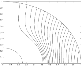
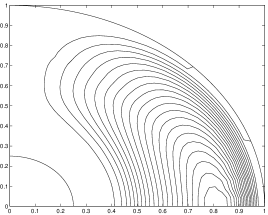
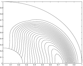
Figure 3: Field configurations corresponding to bottom panel of figure 2, at intermediate times starting from the initial configuration of top left-hand panel. The panels top right, bottom left and bottom right panels correspond to $t=0.015,0.05,0.1$ respectively.

The most interesting conclusion of our work is the fact that the screening becomes progressively less effective with the decreasing strength of the surface field as seen if Fig.[2b] and Fig.[3]. As the magnetic field at the surface decreases due to screening, it can no longer channelize the material flow and the accretion becomes more and more spherical. Magnetic field on the surface of a spherically accreting star is not subject to dragging and subsequent burial. Therefore, after an initial rapid decrease, the decay slows down and the field reaches an asymptotic value as the accretion becomes completely spherical. It should be mentioned here that similar conclusions were drawn by Konar & Bhattacharya (1997) for the case of crustal currents undergoing accretion-induced ohmic dissipation where a purely spherical accretion was assumed to be operative at all times, even though the detailed crustal micro-physics, responsible for such behaviour, has not been incorporated in the screening model. Therefore, further investigation is needed to be undertaken by combining the effects of screening and ohmic dissipation taking into account the detailed micro-physics of the neutron star crust (Konar 2003).

Another important aspect that requires further investigation is the question of the evolution of the screened magnetic field after the cessation of accretion. The effect of magnetic buoyancy, causing the field to re-emerge to the surface would be significant only if the flux resides in the topmost liquid layers. Similarly, ohmic dissipation of the field would be most effective in the outermost layers by virtue of smaller conductivity. It has been seen (Konar & Bhattacharya 1999a, 199b) that for purely spherical accretion by the time accretion ceases, for almost all realistic binary parameters, any initial current configuration (crustal or core) would be buried deep inside the core of the star preventing any further evolution. Therefore, we do not expect any effective re-emergence of the field. However detailed quantitative estimates are still pending.

The details of the screening model discussed here can be found in Choudhuri & Konar (2002) and Konar & Choudhuri (2002, 2003).

References

- [1] Bhattacharya D., 2002, JAA, 22, 67
- [2] Bisnovatyi-Kogan G. S., Komberg B. V., 1974, SvA, 18, 217
- [3] Blandford R. D., DeCampli W. M., Königl A., 1979, BAAS, 11, 703
- [4] Choudhuri, A. R. and Konar, S., 2002, MNRAS, 332, 933
- [5] Cumming A., Zweibel E., Bildsten L., 2001, ApJ, 557, 958
- [6] Konar S., 1997, PhD Thesis, IISc, Bangalore
- [7] Konar S., Bhattacharya D., 1997, MNRAS, 284, 311
- [8] Konar S., Bhattacharya D., 1999a, MNRAS, 303, 588
- [9] Konar S., Bhattacharya D., 1999b, MNRAS, 308, 795
- [10] Konar S., Bhattacharya D., 2001, In Kouveliotou C., van Paradijs J., Ventura J., editors The Neutron Star - Black Hole Connection, NATO Science Series C, Vol. 267, page 71, Kluwer Academic Publishers
- [11] Konar, S. and Choudhuri, A. R., 2002, BASI, 30, 697
- [12] Konar, S. and Choudhuri, A. R., 2003, astro-ph/0304490
- [13] Konar, S., 2003, in preparation
- [14] Melatos A., Phinney E. S., 2001, PASP, 18, 421
- [15] Romani R. W., 1990, Nat, 347, 741
- [16] Romani R. W., 1995, In van Riper K., Epstein R., Ho C., editors Isolated Pulsars, page 75, Cambridge University Press
- [17] Taam R. E., van den Heuvel E. P. J., 1986, ApJ, 305, 235