Effect of entanglement on geometric phase for multi-qubit states

Abstract

When a multi-qubit state evolves under local unitaries it may obtain a geometric phase, a feature dependent on the geometry of the state’s projective Hilbert space. A correction term to this geometric phase in addition to the local subsystem phases may appear from correlations between the subsystems. We find this correction term can be characterized completely either by the entanglement or completely by the classical correlations for several classes of entangled state. States belonging to the former set are W states and their mixtures, while members of the latter set are cluster states, GHZ states and two classes of bound entangled state. We probe the structures of these states more finely using local invariants and suggest the cause of the entanglement correction is a gauge field like $SL(2,\mathbb{C})$ invariant recently introduced named twist.

1. Introduction

The phenomenon of quantum entanglement has received widespread attention recently as researchers have recognized its importance in quantum information theory. Beyond two qubits not much is known about entanglement. Its characterization and quantification becomes particularly hard as the number of possibilities a multi-qubit system can be entangled grows with the number of qubits. For a comprehensive review of entanglement see [1] and references within.

Previous workers have studied the geometric phases of entangled states, mainly restricted to two qubits in a pure state [2, 3, 4, 5, 6]. The geometric phase is a well understood and celebrated effect resulting from the geometry of the state’s projective Hilbert space [7]. In this paper we study the effect multi-qubit entanglement has on the geometric phase in an attempt to distill the geometric features of entanglement. We imagine an entangled $N$ qubit state where each of the $N$ qubits are spatially separated and are in the possession of $N$ parties. Each party may only perform (local) unitaries, analogous to local gauge transformations, on their own qubit. In this way the entanglement and nonlocal properties of the state must remain fixed but it may still obtain a geometric phase dependent on the geometry of its projective Hilbert space. We examine the difference entanglement makes to this phase and therefore to this geometry. Our hope is to elucidate which of the plethora of entanglement structures possible in multi-qubit systems characterized by locally invariant functions of the state parameters are responsible for altering this geometry.

In particular we attempt to understand the following observation: Quantum or classical correlations between subsystems in a composite state modify the geometric phase under local unitary evolution. Stated another way the overall geometric phase of a correlated state $\Gamma$ cannot be written as the sum of its parts, there is a correction term dubbed the mutual geometric phase $\Delta\gamma$ in addition to the local geometric phases obtained by the individual subsystems we label $\gamma_{n}^{M}$. The subscript $n$ labels indexes each of the $N$ subsystems in the correlated state and the superscript $M$ for mixed refers to the fact that in general the subsystems will be in mixed states described by density matrices. We can write this as

$$\Gamma=\Delta\gamma+\sum_{n=1}^{N}\gamma_{n}^{M}.$$ (1)

This is not true of the other phase in quantum mechanics, the dynamical phase. When we restrict to local unitary evolution, the overall dynamical phase of the correlated state $\Upsilon$ can always be understood as the sum of its subsystem’s dynamical phases $\upsilon_{n}^{M}$. One can verify this from the definition of dynamical phase [8]

$$\Upsilon=-i\int_{0}^{T}\hbox{tr}[\rho\mathcal{U}(t)^{\dagger}\dot{\mathcal{U}}(t)]dt$$ (2)

and the local unitary condition $\mathcal{U}(t)=\bigotimes_{n=1}^{N}U_{n}(t)$. Differentiating $\mathcal{U}(t)$ with respect to $t$ and plugging it back into the equation for dynamical phase we find

$$\Upsilon=\sum_{n=1}^{N}\upsilon_{n}^{M}.$$ (3)

We have not assumed anything about the composite state $\rho$, it can be completely general; entangled, classically correlated or uncorrelated. Correlations of any type make no difference. This statement can be seen to be trivial when we regard the local unitaries to effectively model local dynamics. In restricting the dynamics to be local we see the composite dynamical phase can also be thought of as local. In contrast, it can also be seen the geometric phase given by the equation [8]

$$\Gamma=\arg\{\hbox{tr}\rho\mathcal{U}^{\shortparallel}(T)\}$$ (4)

is modified by correlations under the local unitary condition. An uncorrelated, product state $\rho=\bigotimes_{n=1}^{N}\rho_{n}$ can however be written as the sum of its local, subsystem phases as one would expect. $\mathcal{U}^{\shortparallel}$ is the unitary implementing parallel transport on a given path. We will explain what this means in more detail in section 2.1.

Using ideas from entanglement distance measures we can determine which correlations are responsible for this modification of the geometric phase. Correlations are divided into the two coarsest categories by these measures: quantum correlations (entanglement) and classical correlations. From these ideas we calculate three geometric phases associated to a given state (i) the geometric phase of the composite entangled state (ii) the geometric phase of the closest separable state, the state with only the classical correlations between subsystems present and (iii) the geometric phase of the uncorrelated state, that is the composite entangled state with all correlations removed. By comparing these phases we can see what effect the entanglement and the classical correlations have on the geometric phase and therefore the geometry of the projective state space. This is explained in section 2.2.

As entanglement is defined in distance measures as being the surplus correlation not able to be described by classical correlations alone one would intuitively believe that $\Delta\gamma$ can be attributed to a mixture of both entanglement and classical correlations. We find however that the states analyzed belong to one of two sets: the modification $\Delta\gamma$ is due only to entanglement or the modification $\Delta\gamma$ is due only to the classical correlations. We find that W like states and mixtures of W and W̄ states belong to the former set while Greenberger-Horne-Zeilinger (GHZ) states, cluster and two types of bound entangled state, those of Dür and Smolin belong to the latter set. We also find that for pure states of two qubits the mutual geometric phase $\Delta\gamma$ is always accounted for by classical correlations. For entanglement to affect the geometry of the projective state space one at least needs composite states of three qubits or more. First we review and extend previous work [9] using these ideas in section 2.3. and present new analysis in section 3.

In an attempt to understand which features of an entangled state may be responsible for these results we look at the local invariants of the state. That is the things about the entangled state that do not change under local unitaries like the amount of entanglement for instance. It is known that there is only one local invariant of a two pure qubit state, it characterizes the amount of entanglement in the state. For three or more qubits the structures get much richer. One needs five local invariants to describe an arbitrary pure state of three qubits $a$, $b$ and $c$, only four of which have a clear meaning. Three can be thought of as the bipartite entanglements; how entangled $a$ is with $b$, $b$ with $c$ and $c$ with $a$. There is also the 3-tangle, how entangled $a$, $b$ and $c$ are together in a three way correlation and lastly there is the Kempe invariant which seems to have a more geometrical origin following some recent work [10]. We calculate and compare these invariants for the various states in the hope of shedding some light on the cause of two distinct results. In section 4. we show evidence that a local invariant named twist, a function of the Kempe invariant, may be the cause of the modification of geometric phase when entanglement is responsible before finally concluding.

2. Correlations responsible for the difference in geometric phase

In this section we review the core of the analysis, how we characterize $\Delta\gamma$. These calculation are illustrated in detail for GHZ and W state, two inequivalent forms of entanglement under stochastic local operations and classical communication (SLOCC) [11], structures first appearing in pure states of three qubits. First we will review mixed state parallel transport conditions from which one may obtain geometric phases.

2.1. Mixed state parallel transport conditions and geometric phases

If at each neighboring point along a state’s path it is in phase with itself any global phase obtained will be purely geometrical in origin. Moving a state around in this manner is known as parallel transport. Non-trivial parallel transport around a closed loop indicates the space over which the parallel transport is taking place has some curvature. In the case of pure quantum states, parallel transport effectively means no dynamical phase is obtained over the path taken. For clarity, once a pure state $|\psi\rangle$ completes a closed path parameterized by $t$ in projective Hilbert space by the unitary $U(t)$ it will have picked up a global phase $e^{i(\gamma+\upsilon)}|\psi\rangle$. If the state is parallel transported over this path, the dynamical phase $\upsilon=0$ and one is left only with the geometric phase $\gamma$. Mathematically the condition for parallel transport can be written $\langle\psi|U(t)^{\dagger}\dot{U}(t)|\psi\rangle=0$. We write the unitary that fulfills these parallel transport conditions $U^{\shortparallel}$(t).

One can also define parallel transport conditions for mixed states in which case there are multiple choices. We work with the stronger parallel transport condition of [8]. These conditions are known to produce a geometric phase that is a property of the mixed state alone [12] and require each eigenvector $|\phi_{i}\rangle$ of the mixed state $\rho=\sum_{i}\lambda_{i}|\phi_{i}\rangle\langle\phi_{i}|$ to be parallel transported i.e.

$$\langle\phi_{i}|U(t)^{\dagger}\dot{U}(t)|\phi_{i}\rangle=0,\forall i.$$ (5)

Once we have parallel transported a state we know its total overall phase will be the geometric phase. In this case we can use eq. (4), the equation for the total phase, to calculate its geometric phase. Eq. (4) will be used to calculate geometric phases in all the following analysis. Incidentally this formula is valid for all paths, not just closed, cyclic evolutions but in this paper we will parallel transport each subsystem of the entangled state cyclically.

As an example how one might calculate a specific geometric phase associated to a particular Hamiltonian and path imagine a qubit in the state $|0\rangle$ precessing around an axis at angle $\theta$ to the $z$ axis in the $x-z$ plane on the Bloch sphere at frequency $\omega$. The Hamiltonian corresponding to this precession in the $|0\rangle$, $|1\rangle$ basis is

$$H=\frac{\omega}{2}\left(\begin{array}[]{cc}\cos\theta&\sin\theta\\ \sin\theta&-\cos\theta\\ \end{array}\right).$$ (6)

The unitary is then $U(t)=e^{-iHt}$ however this is not the unitary that implements parallel transport. To find this we need to consider which set of unitaries trace the same path in the projective Hilbert space for a given mixed state $\rho=\sum_{i}^{d}\lambda_{i}|\phi_{i}\rangle\langle\phi_{i}|$. It is the set

$$\tilde{U}(t)=U(t)V(t).$$ (7)

$V(t)$ is a unitary that commutes with $\rho$ i.e. $[V(t),\rho]=0$. One can verify $\tilde{U}(t)\rho\tilde{U}(t)^{\dagger}=U(t)\rho U(t)^{\dagger}$ i.e. they both trace the same path. In the case of a mixed state with non-degenerate eigenvalues the most general $V(t)$ is

$$V(t)=\sum_{i}^{d}e^{i\varphi_{i}(t)}|\phi_{i}\rangle\langle\phi_{i}|.$$ (8)

This gauge transformation belongs to the group $U(1)^{d}$ written in the eigenbasis of the density matrix. In the case of a degenerate density matrix with degeneracy $m$ the symmetry group of the gauge transformation that results in the same path is enhanced to $U(m)\times U(1)^{d-m}$. As an example imagine the three level density matrix $\rho=|0\rangle\langle 0|+|1\rangle\langle 1|+2|2\rangle\langle 2|$. This state traces the same path not only with $V(t)$ given by eq. (8) ($U(1)\times U(1)\times U(1)$) but also under the group $U(2)\times U(1)$. The resulting geometric phase factor will then be non-abelian, see [13] for further details. Ultimately the symmetries are determined by the physics of the problem and in this study where we imagine each qubit subsystem to be parallel transported, spatially separated from the others, we have at most $U(2)$ gauge symmetries when the subsystems are maximally mixed. Even when these cases occur we will restrict to symmetries given by eq. (8). In other words we will calculate geometrical, gauge invariant $(U(1)\times U(1))^{N}$ structures of the projective Hilbert space, $N$ being the number of qubits in the state.

Restricting to this abelian case, we need to find the $\tilde{U}(t)$ that implements parallel transport by solving for $\varphi_{i}(t)$ using the parallel transport conditions. This results in the parallel transporter being

$$U^{\shortparallel}(t)=U(t)\sum_{i}^{d}e^{-\int_{0}^{t}\langle\phi_{i}|U(t^{\prime})^{\dagger}\dot{U}(t^{\prime})|\phi_{i}\rangle dt^{\prime}}|\phi_{i}\rangle\langle\phi_{i}|.$$ (9)

One can verify that this choice of $U(t)$ results in a $V(t)$ invariant geometric phase. For the specific Hamiltonian and state $|0\rangle$ considered in this example the geometric phase after a cyclic evolution, $T=2\pi/\omega$ is

$$\gamma=\arg\langle 0|U^{\shortparallel}(T)|0\rangle=\arg\{\langle 0|U(T)|0\rangle e^{-\int_{0}^{T}\langle 0|U^{\dagger}(t)\dot{U}(t)|0\rangle dt}\}$$

$$=-\pi(1-\cos\theta).$$ (10)

The geometric phase is proportional to the area enclosed by the path and in figure 1 we have illustrated this example. In the work that follows we will work more generally without referring to a specific Hamiltonian, making the identifications

$$\langle 0_{n}|U_{n}^{\shortparallel}(T)|0_{n}\rangle=e^{i\gamma_{n}}$$ (11)

$$\langle 1_{n}|U_{n}^{\shortparallel}(T)|1_{n}\rangle=e^{-i\gamma_{n}}$$ (12)

where $n$ refers to the subsystem. The $\pm\gamma_{n}$ are the geometric phases the pure states $|0\rangle$ and $|1\rangle$ obtain over the arbitrary cyclic evolution $U_{n}(T)$. Alternatively one can view $\gamma_{n}$ as half the solid angle enclosed by the path of $|0_{n}\rangle$. One can verify that the state $|1\rangle$ does indeed pick up an equal and opposite geometric phase to $|0\rangle$. By looking at figure 1 one can see that this must be the case. The unitary preserves the scalar product between states and since $|0\rangle$ and $|1\rangle$ are orthogonal, $|1\rangle$ must trace the same path as $|0\rangle$ on the opposite side of the Bloch sphere but in the anti-clockwise rather than clockwise direction giving the minus sign. One notes that this type of structure described by just one parameter, $\gamma$, will not be present for subsystems with more than two levels.

Fig. 1: Cyclic evolution of the state $|0\rangle$ for the Hamiltonian in eq. (6) on the Bloch Sphere. The state $|0\rangle$ is represented by the North pole and the black line traces the path the state makes during its evolution. The solid angle enclosed by the path $|0\rangle$ sweeps out illustrated by the shaded area, $\Omega$, is proportional to the geometric phase, $\gamma$. On the unit Bloch sphere $\gamma=\Omega/2$. For this example the angle of the precession axis from the $z$ axis is $\theta=\pi/4$.

2.2. Determining which correlations are responsible for the mutual geometric phase

Our next step is to determine which correlations are responsible for $\Delta\gamma$ in the expression

$$\Gamma=\Delta\gamma+\sum_{n=1}^{N}\gamma_{n}^{M}.$$ (13)

We can do this by calculating three geometric phases. (i) The geometric phase of the entangled state $\Gamma$ (ii) the geometric phase of the closest separable state (just classical correlations) $\Gamma_{sep}$ and (iii) the geometric phase of the uncorrelated state, the subsystem states tensored together $\sum\gamma_{n}^{M}$. By splitting $\Delta\gamma$ into entanglement $\Delta\gamma_{q}$ and classical correlation $\Delta\gamma_{c}$ contributions so that $\Delta\gamma=\Delta\gamma_{q}+\Delta\gamma_{c}$ we see which correlations contribute to $\Delta\gamma$. Defined in this way the difference entanglement makes to the geometric phase is

$$\Delta\gamma_{q}=\Gamma-\Gamma_{sep}.$$ (14)

Likewise we can see the difference classical correlations make to the geometric phase using

$$\Delta\gamma_{c}=\Gamma_{sep}-\sum_{n=1}^{N}\gamma_{n}^{M}.$$ (15)

In other words the difference between the geometric phases of the maximally classically correlated state and the uncorrelated, product state obtained by tracing each of the subsystems out of our entangled state.

How do we find the closest separable state, $\sigma$? This is the state from the set of all separable states, $S_{sep}$, that minimizes the relative entropy between it and the entangled state, $\rho$. The relative entropy of entanglement, $E_{R}$, is defined as this minimum [14]

$$E_{R}=\min_{\sigma\in S_{sep}}\hbox{tr}\left(\rho\log\rho-\rho\log\sigma\right).$$ (16)

It is probably the most fundamental of a family of entanglement measures called entanglement distance measures. The idea of these measures is that entanglement is defined as the minimum surplus correlation that cannot be accounted for just by classical correlations. The state $\sigma$ replicates as much of the correlation in $\rho$ as possible while only being allowed to be separable. A schematic of this idea is shown in figure 2. These measures are attractive as they apply to systems of any dimension (any number of qu$d$its). The information they provide however is quite coarse, telling you only how much entanglement is in a given state and not the character of the entanglement (they will not tell you whether the entanglement is bipartite/tripartite etc). Distance measures are not easy to calculate either. The hard part of the problem is finding the state that minimizes the given distance measure. This is also the factor that constrains the work in this paper to the classes of entangled states with known $\sigma$.

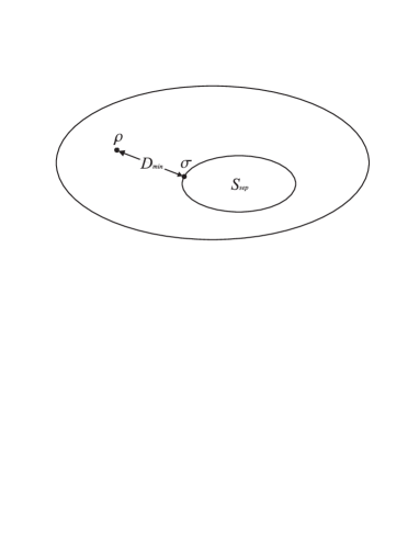
Fig. 2: The boundary of the set of all states is the outermost one. The inner set is the set of all separable states. The two points $\rho$ and $\sigma$ are the entangled state and the closest separable state respectively. The amount of entanglement in $\rho$ is given by the minimum distance $D_{min}$ between itself and the closest point on the set of separable states, $\sigma$. $D$ can be any measure, for the relative entropy of entanglement the measure is the relative entropy and $D_{min}=E_{R}$.

2.3. Geometric phases for GHZ and W states

We now calculate geometric phases and characterize $\Delta\gamma$ for the GHZ and W states. We write the $N$ qubit GHZ state as

$$|GHZ\rangle=\alpha|0\rangle^{\otimes N}+\beta|1\rangle^{\otimes N}.$$ (17)

$\alpha$ and $\beta$ can be made real without loss of generality by making local transformations. GHZ states only have entanglement at the full $N$ qubit level. Once a single qubit is lost the state is separable. W states on the other hand remain entangled down to the last pair of qubits. Our W state is more general than what is usually referred to as a W state in the literature. These states will be written $|N,k\rangle$ where $N$ refers to the number of qubits and $k$ refers to how many are in the state $|1\rangle$. The states are an equal symmetric superposition of all possible distinct permutations.

$$|N,k\rangle=\frac{1}{\sqrt{{\footnotesize\left(\begin{array}[]{c}N\\ k\\ \end{array}\right)}}}\hat{S}|\underbrace{000}_{N-k}....\underbrace{111}_{k}\rangle,$$ (18)

$\hat{S}$ is the complete symmetrization operator. As an example the familiar W state is written $|3,1\rangle=\frac{1}{\sqrt{3}}(|100\rangle+|010\rangle+|001\rangle)$.

First we compute the composite geometric phases for these states using eq. (4) under the conditions that the subsystems are parallel transported according to the mixed state conditions eq. (5) and the evolution of the subsystems is cyclic meaning each subsystem comes back to the same ray for example $|0\rangle=U^{\shortparallel}(T)|0\rangle$ up to a phase factor. We will parallel transport each of the subsystems locally so

$$\mathcal{U}^{\shortparallel}(t)=\bigotimes_{n=1}^{N}U_{n}^{\shortparallel}(t)$$ (19)

where $U_{n}(t)\in SU(2)$. For the GHZ state we have

$$\Gamma_{GHZ}=\arg\left\{\alpha^{2}\prod_{n=1}^{N}\langle 0|U_{n}^{\shortparallel}(T)|0\rangle+\beta^{2}\prod_{n=1}^{N}\langle 1|U_{n}^{\shortparallel}(T)|1\rangle\right\}$$

$$=\arg\left\{\alpha^{2}e^{i\sum_{n=1}^{N}\gamma_{n}}+\beta^{2}e^{-i\sum_{n=1}^{N}\gamma_{n}}\right\},$$ (20)

and for the W state

$$\Gamma_{W}=\arg\left\{\frac{1}{\footnotesize\left(\begin{array}[]{c}N\\ k\\ \end{array}\right)}\sum_{m=1}^{\tiny\left(\begin{array}[]{c}N\\ k\\ \end{array}\right)}e^{i\sum_{n=1}^{N}A_{mn}\gamma_{n}}\right\}.$$ (21)

In the equation for $\Gamma_{W}$ we have introduced the ${\tiny\left(\begin{array}[]{c}N\\ k\\ \end{array}\right)}$ by $N$ matrix $A$ to capture the sign of $\gamma_{n}$. Each row has $N-k$ elements that are $1$ and $k$ elements being $-1$. Each row is a distinct permutation of the elements of this first row.

Next we calculate the local, subsystem geometric phases, $\gamma_{n}^{M}$, of the two states. To do this we first find the subsystem states, $\rho_{n}$, by tracing out all but the subsystem from $|GHZ\rangle$ or $|N,k\rangle$ we are interested in. Because of the permutation symmetry all the $N$ subsystems have the same state.

$$\rho_{n}^{GHZ}=\alpha^{2}|0\rangle\langle 0|+\beta^{2}|1\rangle\langle 1|,$$ (22)

$$\rho_{n}^{W}=\frac{N-k}{N}|0\rangle\langle 0|+\frac{k}{N}|1\rangle\langle 1|.$$ (23)

From these subsystem states we can calculate the local subsystem phases of the uncorrelated ($uc$) state $\rho^{uc}=\bigotimes_{n=1}^{N}\rho_{n}$, the local geometric phases $\sum\gamma_{n}^{M}$. For the GHZ state we have

$$\left(\sum_{n=1}^{N}\gamma_{n}^{M}\right)^{GHZ}=\sum_{n=1}^{N}\arg\left\{\alpha^{2}e^{i\gamma_{n}}+\beta^{2}e^{-i\gamma_{n}}\right\}$$

$$=\arg\left\{\prod_{n=1}^{N}\alpha^{2}e^{i\gamma_{n}}+\beta^{2}e^{-i\gamma_{n}}\right\},$$ (24)

and the W state

$$\left(\sum_{n=1}^{N}\gamma_{n}^{M}\right)^{W}=\arg\left\{\prod_{n=1}^{N}\frac{N-k}{N}e^{i\gamma_{n}}+\frac{k}{N}e^{-i\gamma_{n}}\right\}$$

$$=\arg\left\{\frac{1}{N^{N}}\sum_{l=0}^{N}(N-k)^{N-l}k^{l}\sum_{m=1}^{\tiny\left(\begin{array}[]{c}N\\ l\\ \end{array}\right)}e^{i\sum_{n=1}^{N}A^{l}_{mn}\gamma_{n}}\right\}.$$ (27)

In the last equation we have constructed another matrix $A^{l}$ similar to our last $A$ matrix in eq (21). The difference is that the rows of $A^{l}$ have $N-l$ elements with the value $1$ and $l$ elements with the value $-1$. Again, the other ${\tiny\left(\begin{array}[]{c}N\\ l\\ \end{array}\right)}-1$ rows are the distinct permutations of the first row.

We also calculate the geometric phase of the other relevant state, the closest separable state, $\sigma$. For the GHZ and W state these closest separable states are known. They are given by [15, 16]

$$\sigma^{GHZ}=\alpha^{2}|0\rangle\langle 0|^{\otimes N}+\beta^{2}|1\rangle\langle 1|^{\otimes N},$$ (28)

$$\sigma^{W}=\frac{1}{N^{N}}\sum_{l=0}^{N}\left(\begin{array}[]{c}N\\ l\\ \end{array}\right)(N-k)^{N-l}k^{l}|N,l\rangle\langle N,l|.$$ (29)

The geometric phases for these states are

$$\Gamma_{sep}^{GHZ}=\arg\left\{\alpha^{2}e^{i\sum_{n=1}^{N}\gamma_{n}}+\beta^{2}e^{-i\sum_{n=1}^{N}\gamma_{n}}\right\},$$ (30)

$$\Gamma_{sep}^{W}=\arg\left\{\frac{1}{N^{N}}\sum_{l=0}^{N}(N-k)^{N-l}k^{l}\sum_{m=1}^{\tiny\left(\begin{array}[]{c}N\\ l\\ \end{array}\right)}e^{i\sum_{n=1}^{N}A^{l}_{mn}\gamma_{n}}\right\}.$$ (31)

We now have all the ingredients necessary to characterize $\Delta\gamma$. For GHZ states one finds

$$\Gamma^{GHZ}=\Gamma_{sep}^{GHZ}$$ (32)

so that $\Delta\gamma^{GHZ}=\Delta\gamma_{c}^{GHZ}$ and $\Delta\gamma_{q}^{GHZ}=0$. For GHZ states classical correlations are solely responsible for the change in the geometric phase above the local phases. Since all pure two qubit states can be cast in the form of a GHZ state by local transformations, this statement is also true of all two qubit pure states.

For W states one finds the polar opposite

$$\Gamma_{sep}^{W}=\left(\sum_{n=1}^{N}\gamma_{n}^{M}\right)^{W}$$ (33)

so that $\Delta\gamma^{W}=\Delta\gamma^{W}_{q}$ and $\Delta\gamma_{c}^{W}=0$. For W states entanglement is solely responsible for the change in the geometric phase above the local phases.

For GHZ states when $\alpha=\beta$ and when $k=N/2$ for W states all geometric phase factors are $1$ or $-1$, elements of $\mathbb{Z}_{2}$ giving phases of 0 or $\pi$. This happens because the functions inside the argument in eq. (4) become real. Incidently this occurs when $E_{R}$ is maximal for these states. In this paper we will term geometric phase factors in $\mathbb{Z}_{2}$ as trivial.

3. Other states: Bound entangled, W mixtures and cluster states.

The results from the last section are intriguing and also rather mysterious. Since both classes of state contained both entanglement and classical correlations one might have suspected that this would have been reflected in type of correlation responsible for the difference in the geometric phase. However we found two extreme cases; the difference in W states was described purely by the entanglement and for GHZ states it was described purely by the classical correlations. In this section we investigate other entangled states for which the closest separable states are known. The aim being to pick out the features responsible for this result. We calculate for the interesting classes of cluster states, the bound entangled states of Dür and Smolin and mixtures of W states. As in the last section we find these new classes of state can also be categorized as having a either a geometric phase difference arising solely from entanglement or classical correlations. We group these two sets in the following subsections. Note that many of the states we write down are unnormalized.

3.1. $\Delta\gamma=\Delta\gamma_{c}$: State geometries described by classical correlation

3.1.1. Cluster states

Cluster states first appear for four qubit spaces and form a new SLOCC class [17]. They are interesting because they have properties somewhere in the middle of GHZ and W states [18], remaining entangled until $N/2$ of the particles are traced out.

One may create a $N$ qubit cluster state, $|\varphi^{N}\rangle$, by taking $N$ pure qubits each in the state $|0\rangle+|1\rangle$ and applying a controlled phase gate (CZ) between neighbors. The CZ in the $|0\rangle$, $|1\rangle$ basis is the $4\times 4$ matrix $diag\{1,1,1,-1\}$. Here we consider linear cluster states, states where CZs are applied between qubits $1$ and $2$, $2$ and $3$ etc. The first five of these states (up to local unitary transforms) are given by

$$|\varphi^{2}\rangle=|00\rangle+|11\rangle$$ (34)

$$|\varphi^{3}\rangle=|000\rangle+|111\rangle$$ (35)

$$|\varphi^{4}\rangle=|0000\rangle+|0111\rangle+|1011\rangle+|1100\rangle$$ (36)

$$|\varphi^{5}\rangle=|00000\rangle+|00111\rangle+|11011\rangle+|11100\rangle$$ (37)

$$|\varphi^{6}\rangle=|000000\rangle+|000111\rangle+|011011\rangle+|011100\rangle...$$

$$+|101011\rangle+|101100\rangle+|110000\rangle+|110111\rangle.$$ (38)

The two and three qubit states are equivalent to Bell and GHZ states respectively while the four qubit state is distinct. If we trace qubits out of the $N\geq 4$ cluster states to obtain a 3 qubit state we find some partitions are entangled. One can verify this using the Peres-Horodecki criterion [19, 20] by transposing one of the qubits and checking if the resulting matrix is no longer positive. Strangely, we find that even though the state is entangled it has no bipartite or tripartite entanglement as defined by the 2- and 3-tangles (see section 4.). It is another example of an entangled mixed three qubit state having no 2- or 3-tangle in addition to those found by [21].

The general method for finding the closest separable states is given in [22]. Using this method we can construct the closest separable state to $|\varphi^{N}\rangle$. Here we give the closest state to $|\varphi^{4}\rangle$

$$\sigma^{4}=|0000\rangle\langle 0000|+|0111\rangle\langle 0111|...$$

$$+|1011\rangle\langle 1011|+|1100\rangle\langle 1100|.$$ (39)

The other closest states may be constructed from $|\varphi^{N}\rangle\langle\varphi^{N}|$ simply by removing the off-diagonal terms in the $|0\rangle$, $|1\rangle$ basis. Each of the $N$ subsystems are given by the maximally mixed state

$$\rho_{n}=|0\rangle\langle 0|+|1\rangle\langle 1|.$$ (40)

One can verify that $\Gamma=\Gamma_{sep}$ and therefore $\Delta\gamma=\Delta\gamma_{c}$. Also notice that the local geometric phase factors are always trivial. The geometric phase factors of the entangled and closest separable states can however be complex giving a continuum of possible phases.

3.1.2. Smolin’s unlockable bound entangled state

In [23] Smolin presented a 4 qubit bound entangled state. Bound entangled meaning that no pure state entanglement may be distilled from the state by LOCC. It is termed unlockable because when two parties come together a Bell state may be obtained by the other two parties using only LOCC. The state is

$$\rho^{Smolin}=\frac{1}{4}\sum_{i=0}^{3}|X_{i}\rangle\langle X_{i}|$$ (41)

where $|X_{0}\rangle=|0000\rangle+|1111\rangle$, $|X_{1}\rangle=|0011\rangle+|1100\rangle$, $|X_{2}\rangle=|0101\rangle+|1010\rangle$ and $|X_{3}\rangle=|0110\rangle+|1001\rangle$ are GHZ states. Once a qubit is removed the state is separable. The closest separable state to $\rho^{Smolin}$ has been given by [24] and is obtained again by removing the off-diagonal elements in this basis. Each subsystem is given by the maximally mixed state and a straight forward calculation reveals that $\Gamma=\Gamma_{sep}$. For this state all geometric phase factors are trivial.

3.1.3. Dür’s bound entangled state

Dür found a state that demonstrated bound entanglement does not necessarily imply one can find a local hidden variable model (LHV) describing the state [25]. The violation of a Bell type inequality indicates the non-existence of a LHV and the state Dür presented violated such an inequality for $N\geq 8$. It was also demonstrated that for $N\geq 4$ the following state is bound entangled

$$\rho^{D\ddot{u}r}=x|GHZ\rangle\langle GHZ|+\frac{1-x}{2N}\sum_{k=1}^{N}P_{k}+\bar{P}_{k}$$ (42)

for $x=1/(N+1)$. Wei et al. [24] show that this state is bound entangled for $0<x\leq 1/(N+1)$ and entangled for $x>1/(N+1)$. $|GHZ\rangle=(|0\rangle^{\otimes N}+|1\rangle^{\otimes N})/\sqrt{2}$ and $P_{k}=|0\rangle_{1}|0\rangle_{2}|0\rangle_{3}...|1\rangle_{k}...|0\rangle_{N}$ i.e. a projector composed of $|0\rangle$s but with $|1\rangle$ in the $k$th qubit position. $\bar{P}_{k}$ is similar except $\bar{P}_{k}=|1\rangle_{1}|1\rangle_{2}|1\rangle_{3}...|0\rangle_{k}...|1\rangle_{N}$. Dür’s state is a mixture of an $N$ qubit GHZ state and collection of separable states and the loss of a qubit renders it separable. The closest separable state has been given by Wei [26] for $N\geq 4$

$$\sigma^{D\ddot{u}r}=\frac{x}{2}\left(|0\rangle\langle 0|^{\otimes N}+|1\rangle\langle 1|^{\otimes N}\right)+\frac{1-x}{2N}\sum_{k=1}^{N}P_{k}+\bar{P}_{k}.$$ (43)

This state is the same as the closest to the pure GHZ state mixed with the separable part of $\rho^{D\ddot{u}r}$. Single qubit subsystems are maximally mixed states, $\Gamma=\Gamma_{sep}$ and all geometric phase factors are trivial.

3.2. $\Delta\gamma=\Delta\gamma_{q}$: State geometries described by entanglement

3.2.1. Mixtures of W and W̄ bar states

The W states we consider here are the more traditional ones, in our notation $|W\rangle=|N,1\rangle$ and $|\bar{W}\rangle=|N,N-1\rangle$. We consider $N$ qubit mixtures of these two states

$$\rho^{\bar{W}}=p|W\rangle\langle W|+(1-p)|\bar{W}\rangle\langle\bar{W}|.$$ (44)

Recently it has been shown that equal mixtures ($p=1/2$) of odd $N$ have no $N$ party classical correlations in the sense that all elements of the $N$ party correlation tensor $\langle\sigma^{1}_{i_{1}}\sigma^{2}_{i_{2}}...\sigma^{N}_{i_{N}}\rangle=0$. The indices $i_{n}$ can take the values $x$, $y$ or $z$. However it was also shown that $\rho^{\bar{W}}$ has $N$ party entanglement meaning there is no partitioning that can be written as a separable state [27]. The closest separable state has been found by [26] for a larger class, states of the form $\sum_{k}p_{k}|N,k\rangle\langle N,k|$. In general these $\sigma$ cannot be written down in closed form, also true for $\rho^{\bar{W}}$ for any $N$. We can however write the closest separable states for $N=3,4$ in closed form. They are

$$\sigma^{\bar{W}}=\frac{1}{N^{N}}\sum_{l=0}^{N}\begin{pmatrix}N\\ l\\ \end{pmatrix}\alpha^{l}(N-\alpha)^{N-l}|N,l\rangle\langle N,l|$$ (45)

where $\alpha=p+(N-1)(1-p)$. The individual subsystems are given by

$$\rho_{n}=\frac{N-\alpha}{N}|0\rangle\langle 0|+\frac{\alpha}{N}|1\rangle\langle 1|.$$ (46)

In the same way as we proceeded for pure W states in section 2. one can show $\Gamma_{sep}=\sum_{n=1}^{N}\gamma_{n}^{M}$. Only entanglement modifies the geometric phase. When $p=1/2$ all geometric phase factors are trivial. Presumably for $N\geq 5$ when the closest separable state becomes difficult to write down classical correlations become important in describing $\Delta\gamma$.

3.2.2. States resulting from tracing qubits out from $|N,k\rangle$

One can also consider mixtures of symmetric states resulting from tracing qubits out of $|N,k\rangle$. Provided we consider states of $m\leq k\leq N-m$ qubits we have the entangled state

$$\rho^{m}=\sum_{l=0}^{m}\begin{pmatrix}m\\ l\\ \end{pmatrix}\frac{\tiny\begin{pmatrix}N-m\\ k-l\\ \end{pmatrix}}{\tiny\begin{pmatrix}N\\ k\\ \end{pmatrix}}|m,l\rangle\langle m,l|.$$ (47)

The closest separable state has been found by [28]

$$\sigma^{m}=\frac{1}{N^{m}}\sum_{l=0}^{m}\left(\begin{array}[]{c}m\\ l\\ \end{array}\right)(N-k)^{m-l}k^{l}|m,l\rangle\langle m,l|.$$ (48)

The subsystems are still given by the same states as the W states in section 2. A similar calculation as the one performed in that section shows $\Gamma_{sep}=\sum_{n=1}^{m}\gamma_{n}^{M}$. When $k=N/2$ all geometric phase factors are trivial.

4. Properties responsible for $\Delta\gamma_{q}$

What are the features of these states that put them either in the $\Delta\gamma=\Delta\gamma_{q}$ or $\Delta\gamma=\Delta\gamma_{c}$ set? Using the geometric phase we have been looking at geometrical properties of the projective Hilbert space invariant under local $U(1)\times U(1)$ gauge transformations. In this section we look at some of the properties of these states invariant under the action of local $SU(2)$ gauge transformations, a higher symmetry group containing $U(1)\times U(1)$. They are also the same transformations we have been making to obtain geometric phases. We actually look at the invariants of the larger local special linear group $SL(2,\mathbb{C})$ because several well known entanglement measures have this higher invariance as well as invariance under $SU(2)$.

In this section we introduce and calculate a full set of $SL(2,\mathbb{C})$ invariants for pure three qubit states. It is a full set in the sense that an arbitrary pure state of three qubits can be determined up to local unitary transforms to a set of two possible states by the values of these invariants [29, 30, 31]. All $SL(2,\mathbb{C})$ invariants we work with here are zero for the closest separable and product states presented in this paper. This indicates these invariants may be useful for discovering the features that make a difference to $\Delta\gamma_{q}$ but will not be useful for identifying the properties responsible for $\Delta\gamma_{c}$.

4.1. Local $SL(2,\mathbb{C})$ invariants

4.1.1. Bipartite entanglement $\tau_{ab}$

To measure bipartite entanglement we will use the square of the concurrence called the 2-tangle. It measures how entangled 2 qubits, $a$ and $b$ are and may be calculated from [32]

$$\tau_{ab}=\max\{0,\lambda_{1}-\lambda_{2}-\lambda_{3}-\lambda_{4}\}^{2}$$ (49)

where $\lambda_{i}$ are the square roots of the eigenvalues of $\rho_{ab}(\sigma_{y}\otimes\sigma_{y})\rho_{ab}^{*}(\sigma_{y}\otimes\sigma_{y})$ put in decreasing order.

All classes of states with $\Delta\gamma=\Delta\gamma_{c}$ have no bipartite entanglement suggesting it might be responsible for $\Delta\gamma_{q}$. In general all $\Delta\gamma=\Delta\gamma_{q}$ states have bipartite entanglement. However there are $\Delta\gamma=\Delta\gamma_{q}$ states with finite bipartite entanglement and trivial geometric phase ($\Delta\gamma=0,\pi$) for example $\rho^{\bar{W}}$ for $N=3$ and $p=1/2$: The 2-tangle for each pair of qubits is $\tau=4/9[1-\sqrt{p(1-p)}]^{2}$. This suggests bipartite entanglement does not uniquely prescribe the state space geometry due to entanglement.

4.1.2. Tripartite entanglement $\tau_{abc}$

For pure three qubit states Coffman et al. introduced the 3-tangle, a measure of how much entanglement there is in three way entanglement between the qubits. The equation for pure state 3-tangle is given in [33]. To extend this notion to mixed three qubit states we follow [21] and define the mixed state entanglement to be the average pure state 3-tangle minimized over all possible decompositions of $\rho=\sum_{i}p_{i}|\psi_{i}\rangle\langle\psi_{i}|$,

$$\tau_{abc}(\rho)=\min\sum_{i}p_{i}\tau_{abc}\left(|\psi_{i}\rangle\langle\psi_{i}|\right).$$ (50)

The expression for bipartite entanglement is defined analogously but has a known closed form.

There is only one state with non-zero 3-tangle, the $N=3$ GHZ state which has $\tau_{abc}=4\alpha^{2}\beta^{2}$. We can exclude 3-tangle as the invariant responsible for $\Delta\gamma_{q}$.

4.1.3. Twist $T(\tilde{a}\tilde{b}\tilde{c})$

This was introduced in [10] as a quantity exhibiting $SL(2,\mathbb{C})$ invariance. They showed strong numerical evidence that this invariant is a function of the Kempe invariant and therefore forms a complete set of local invariants for pure three qubit states when accompanied with the three 2-tangles and 3-tangle. It is interesting as it arises from an approach to generating $SL(2,\mathbb{C})$ and $SU(2)$ invariants inspired by lattice gauge theory. It turns out this is the only non-trivial gauge field like invariant for pure states of three qubits and to calculate it you construct a Wilson loop. The equation is

$$T(\tilde{a}\tilde{b}\tilde{c})=\frac{1}{4}\hbox{tr}\left[U(a,\tilde{c})U(c,\tilde{b})U(b,\tilde{a})\right].$$ (51)

To obtain the unitaries $U(b,a)$ we take the $4\times 4$ correlation matrix $S(b,a)_{ji}=\langle\sigma_{i}^{a}\otimes\sigma_{j}^{b}\rangle$, where $\sigma_{i}$ belong to the set of Pauli matrices $\{\mathbf{I},\sigma_{1},\sigma_{2},\sigma_{3}\}$ and polar decompose it into $U(b,a)=P^{-1}S(b,a)$. $P$ is a positive semi-definite Hermitian matrix given by $\sqrt{S(b,a)S(b,a)^{T}}$. If $S$ is not of full rank then $U$ is not unique and $T(\tilde{a}\tilde{b}\tilde{c})$ is undefined. The tildes denote a spin flip on that particular qubit i.e. $U(b,\tilde{a})=U(b,a)\eta$ where $\eta=diag\{1,-1,-1,-1\}$.

The eigenvalues of $U(a,\tilde{c})U(c,\tilde{b})U(b,\tilde{a})$ are also $SL(2,\mathbb{C})$ invariants generally being complex elements of $U(1)$. However for some states they are real and belong to $\mathbb{Z}_{2}$. This occurs when $T(\tilde{a}\tilde{b}\tilde{c})=1$. We will term $T(\tilde{a}\tilde{b}\tilde{c})=1$ as trivial twist in analogy with our terminology for the geometric phase.

All $\Delta\gamma=\Delta\gamma_{c}$ states have undefined twist making it a candidate for the invariant responsible for $\Delta\gamma_{q}$. This is also supported by the fact $\Delta\gamma_{q}$ states have unique and non-trivial twist when all geometric phases are non-trivial in all the examples considered. To give some examples of values of twist, the state $|3,1\rangle$ has $T(\tilde{a}\tilde{b}\tilde{c})=-0.41$ and $\rho_{\bar{W}}$, $N=3$ takes values between $0$ ($p=1/2$) and $-0.41$ ($p=1$). This suggests that twist is the invariant responsible for $\Delta\gamma_{q}$. We have found no counter example in the states considered.

4.2. Discussion

We have found that twist seems to be the most likely cause of the $\Delta\gamma_{q}$ correction to the geometric phase. It is undefined for all the states with $\Delta\gamma=\Delta\gamma_{c}$ and becomes trivial or undefined when the geometric phase becomes trivial ($\Delta\gamma=0,\pi$). Although we have not found a counter example the results are not conclusive. The set of five $SL(2,\mathbb{C})$ invariants are only complete for pure three qubit states. For mixed states or states with higher numbers of qubits further invariants must be added to completely describe the state up to local unitary equivalence. However, all the $\Delta\gamma=\Delta\gamma_{q}$ states we considered were simple structures that first appear for pure states of three qubits or mixtures of such structures. Provided twist is the invariant giving rise to non-zero $\Delta\gamma_{q}$ one would also like to see the exact mechanism whereby the twist alters the geometric phase.

The other set of states that has $\Delta\gamma=\Delta\gamma_{c}$ are largely four qubit states. We have not been able to identify which invariants are responsible for $\Delta\gamma_{c}$. To do this we could look at the invariants between the entangled state, the closest separable state and the uncorrelated state. These should be the same for the entangled and closest separable states but be different for the uncorrelated state. The $SL(2,\mathbb{C})$ invariant set we have used here are not good for this purpose as they are zero or undefined for all the unentangled states considered. Perhaps a set of $SU(2)$ invariants for 4 qubit states would be useful for this purpose.

5. Conclusion

In this paper we have shown that under the action of local unitaries correlations in a state add corrections to the geometric phase in addition to the local phases obtained by its subsystems. We showed that correlations did not change the other phase in quantum mechanics, dynamical phase.

Of the two types of correlation in quantum mechanics, entanglement and classical correlations, we showed that this correction to the geometric phase could be described entirely by classical correlations for GHZ states, cluster states and two examples of bound entangled state. In contrast we found that this correction could be completely described by entanglement for W states and mixtures of W states.

We investigated what properties of the state may be responsible for the entanglement correction to the geometric phase using local invariants to probe structures of the states more finely. We found one possible candidate for the entanglement correction, this was a quantity called twist, also geometrical in construction and of a possible gauge field like interpretation.

Regarding possible future work, this study restricted the subsystem evolutions to be cyclic, that is each subsystem came back to itself after some arbitrary unitary evolution. It would be interesting to consider the non-cyclic cases. We also restricted the symmetries of the subsystem paths in the projective Hilbert space to be abelian ($U(1)\times U(1)$) even when the subsystems became maximally mixed. When the subsystems become maximally mixed the symmetry becomes elevated to $U(2)$ and one may obtain a non-abelian geometric phase. This may also be interesting to investigate further. It would also be nice to see the exact mechanism that produces these corrections to the geometric phase and identify possible properties that result in the classical correlation correction to the geometric phase.

MSW acknowledges partial funding from EPSRC and QIP IRC www.qipirc.org (GR/S82176/01). We thank Michal Hajdušek for communicating his results on cluster states.

References

- [1] R. Horodecki, P. Horodecki, M. Horodecki, and K. Horodecki. Quantum entanglement. quant-ph/0702225v2, 2007.
- [2] E. Sjöqvist. Geometric phase for entangled spin pairs. Phys. Rev. A, 62:022109, 2000.
- [3] D. M. Tong, E. Sjöqvist, L. C. Kwek, C. H. Oh, and M. Ericsson. Relation between geometric phases of entangled bipartite systems and their subsystems. Phys. Rev. A, 68(2):022106, 2003.
- [4] X. X. Yi and E. Sjöqvist. Effect of intersubsystem coupling on the geometric phase in a bipartite system. Phys. Rev. A, 70(4):042104, 2004.
- [5] B. Basu. Relation between concurrence and Berry phase of an entangled state of two spin 1/2 particles. Europhys. Lett., 73(6):833–838, 2006.
- [6] E. Sjöqvist. Correlation-sensitive geometric phases of a bipartite quantum state. arXiv:0803.2609v2, 2008.
- [7] A. Shapere and F. Wilczek. Geometric Phases in Physics. World Scientific, Singapore, 1989.
- [8] E. Sjöqvist, A. K. Pati, A. Ekert, J. S. Anandan, M. Ericsson, D. K. L. Oi, and V. Vedral. Geometric phases for mixed states in interferometry. Phys. Rev. Lett., 85(14):2845–2849, 2000.
- [9] M. S. Williamson and V. Vedral. Composite geometric phase for multiparticle entangled states. Phys. Rev. A, 76:032115, 2007.
- [10] A. Sudbery, V. Vedral, M. S. Williamson, and W. K. Wootters. Geometric local invariants and three-qubit pure states. unpublished, 2008.
- [11] W. Dür, G. Vidal, and J. I. Cirac. Three qubits can be entangled in two inequivalent ways. Phys. Rev. A, 62(6):062314, 2000.
- [12] M. Ericsson, A. K. Pati, E. Sjöqvist, J. Brannlund, and D. K. L. Oi. Mixed state geometric phases, entangled systems and local unitary transformations. Phys. Rev. Lett., 91(9):090405, 2003.
- [13] K. Singh, D. M. Tong, K. Basu, J. L. Chen, and J. F. Du. Geometric phases for non-degenerate and degenerate mixed states. Phys. Rev. A, 67:032106, 2003.
- [14] V. Vedral, M. B. Plenio, M. A. Rippin, and P. L. Knight. Quantifying entanglement. Phys. Rev. Lett., 78(12):2275, 1997.
- [15] V. Vedral and M. B. Plenio. Entanglement measures and purification proceedures. Phys. Rev. A, 57(3):1619, 1998.
- [16] T. C. Wei, M. Ericsson, P. M. Goldbart, and W. J. Munro. Connections between the relative entropy of entanglement and geometric measure of entanglement. Quantum Inform. Compu., 4(4):252, 2004.
- [17] A. Osterloh and J. Siewert. Constructing -qubit entanglement monotones from antilinear operators. Phys. Rev. A, 72:012337, 2005.
- [18] H. J. Briegel and R. Raussendorf. Persistent entanglement in arrays of interacting particles. Phys. Rev. Lett., 86:910–913, 2001.
- [19] A. Peres. Separability criterion for density matrices. Phys. Rev. Lett., 77(8):1413–1415, 1996.
- [20] M. Horodecki, P. Horodecki, and R. Horodecki. Separability of mixed states: Necessary and sufficient conditions. Phys. Lett. A, 223:1–8, 1996.
- [21] R. Lohmayer, A. Osterloh, J. Siewert, and A. Uhlmann. Entangled three-qubit states without concurrence and three-tangle. Phys. Rev. Lett., 97:260502, 2006.
- [22] M. Hajdušek and V. Vedral. Entanglement in one-dimensional thermal cluster chains. arXiv:0902.4343, 2009.
- [23] J. A. Smolin. Four-party unlockable bound entangled state. Phys. Rev. A, 63:032306, 2001.
- [24] T. C. Wei, J. B. Altepeter, P. M. Goldbart, and W. J. Munro. Measures of entanglement in multipartite bound entangled states. Phys. Rev. A, 70:022322, 2004.
- [25] W. Dür. Multipartite bound entangled states that violate Bell’s inequality. Phys. Rev. Lett., 87(23):230402, 2001.
- [26] T. C. Wei. Relative entropy of entanglement for multipartite mixed states: Permutation-invariant states and Dür states. Phys. Rev. A, 78:012327, 2008.
- [27] D. Kaszlikowski, A. Sen(De), U. Sen, V. Vedral, and A. Winter. Quantum correlations without classical correlations. Phys. Rev. Lett., 101:070502, 2008.
- [28] V. Vedral. High-temperature macroscopic entanglement. New J. Phys., 6:102, 2004.
- [29] N. Linden and S. Popescu. On multi-particle entanglement. Fortschr. Phys., 46(4-5):567–578, 1998.
- [30] A. Sudbery. On local invariants of pure three-qubit states. J. Phys. A: Math. Gen., 34:643–652, 2001.
- [31] A. Acìn, A. Andrianov, E. Jané, and R. Tarrach. Three-qubit pure-state canonical forms. J. Phys. A: Math. Gen., 34:6725–6739, 2001.
- [32] W. K. Wootters. Entanglement of formation of an arbitrary state of two qubits. Phys. Rev. Lett., 80(10):2245–2248, 1998.
- [33] V. Coffman, J. Kundu, and W. K. Wootters. Distributed entanglement. Phys. Rev. A, 61(5):052306, 2000.