Zero-temperature dynamics of solid ⁴He
from quantum Monte Carlo simulations

Abstract

The lattice dynamics of hcp crystalline ⁴He is studied at zero temperature and for two different densities (near and far from melting), using a ground-state path-integral quantum Monte Carlo technique. The complete phonon dispersion is obtained, with particular attention to the separation of optic and acoustic branches and to the identification of transverse modes. Our study also sheds light onto the residual coherence affecting quasiparticle excitations in the intermediate momentum region, in-between the phonon and nearly-free particle regimes.

The lattice dynamics of solid ⁴He has long been considered a major challenge to ab initio calculations, due to the strong anharmonicity of this highly quantum solid. Many calculations have been performed within the Self Consistent Phonon (SCP) approximation,Gillis et al. (1968); Glyde (1994) which however may be rather unsatisfactory, due to the magnitude of anharmonic effects. A significant improvement has been made possible by the application of a variational quantum Monte Carlo (QMC) approach, based on the shadow wave function formalism, to bcc ³He Mazzi et al. (2006) and to hcp ⁴He.Galli and Reatto (2003) The variational nature of this approach, however, makes it not fully suitable at high energy where optical or zone-boundary longitudinal excitations exhibit broad multiphonon features. In this spectral regime, the calculation of the full dynamic structure factor is therefore in order. QMC techniques based on path integrals allow quite naturally for the calculation of imaginary-time correlation functions from which various spectral functions, such as the dynamic structure factor, can be obtained upon analytical continuation. This technique has been successfully demonstrated for superfluid ⁴He,Boninsegni and Ceperley (1996); Baroni and Moroni (1999a) as well as for the bcc crystalline phases of ⁴He  Sorkin et al. (2005); Pelleg et al. (2008) and ³He.Sorkin et al. (2006) In the latter studies the spectrum of the transverse excitations has also been obtained, albeit in the one-phonon approximation only.Glyde (1994)

In this work we present an extensive study of the dynamical properties of hcp ⁴He at zero temperature, performed by estimating the dynamic structure factor from ground-state path-integral simulations. Ceperley (1995); Baroni and Moroni (1999a); Sarsa et al. (2000) This technique allows us to parallel to some extent the procedure followed experimentally to map phonon dispersions from the measured neutron scattering. In the long wave-length region—well approximated by a phonon picture of the collective density excitations—we thus obtain longitudinal as well as transverse modes for both acoustic and optical branches. For higher wave-vectors we analyse the dynamic structure factor in terms of corrections to the so-called impulse approximation,Glyde (1994/09/01/) finding a coherent response which is peculiar of both superfluid and solid helium.

In Sec. I we give an introductory account of the phonon theory of long wave-length excitations in solids. In Sec. II the reader is provided with an outline of the numerical methods adopted in this work. In Sec. III we report on the analysis of our QMC results both in the phonon regime and in the intermediate momentum region. Sec. IV is finally devoted to a few concluding remarks.

I Lattice dynamics

I.1 Long wave-lengths

The long wave-length lattice dynamics of a solid is fully characterized by its dynamic structure factor, which is the space-time Fourier transform of the density-density correlation function. In real time and reciprocal space, the autocorrelation function of the density operator reads:

$$S(\mathbf{Q},t)=\frac{1}{N}\left\langle\sum_{kl}e^{-i\mathbf{Q}\cdot\mathbf{r}_{k}(t)}e^{i\mathbf{Q}\cdot\mathbf{r}_{l}(0)}\right\rangle,$$ (1)

where the brackets indicate equilibrium (ground-state or thermal) expectation values. In a weakly anharmonic system, it is convenient to expand $S(\mathbf{Q},t)$ into a sum of terms involving one-phonon processes, two-phonon scattering, interference processes and so on:Glyde (1994)

$$S(\mathbf{Q},t)=S_{1}(\mathbf{Q},t)+S_{2}(\mathbf{Q},t)+S_{1,2}(\mathbf{Q},t)+\cdots.$$ (2)

The physical meaning of such an expansion is best appreciated by introducing the atomic displacements from the equilibrium lattice sites, $\{\mathbf{R}_{l}\}$: $\mathbf{u}_{l}(t)=\mathbf{r}_{l}(t)-\mathbf{R}_{l}$. In terms of the $\mathbf{u}$’s and the $\mathbf{R}$’s, the one-phonon contribution to the dynamic structure factor of a simple Bravais lattice reads:Glyde (1994)

$$S_{1}(\mathbf{Q},t)=e^{-2W}{\sum_{l}e^{-i\mathbf{Q}\cdot\left(\mathbf{R}_{l}-\mathbf{R}_{0}\right)}}\times\\ \times\left\langle\mathbf{Q}\cdot\mathbf{u}_{l}(t)\mathbf{Q}\cdot\mathbf{u}_{0}(0)\right\rangle,$$ (3)

where $e^{-2W}$ is the Debye-Waller factor. For a harmonic crystal—to which only, strictly speaking, the phonon language applies—we consider the vibrational frequency $\omega_{j}(\mathbf{q})$ and polarization vector $\bm{\epsilon}(\mathbf{q}|j)$ of the $j$-th phonon branch at wave vector $\mathbf{q}$ in the first Brillouin Zone (FBZ). In terms of these quantities, the one-phonon contribution reads:Brockhouse and Iyengar (1958)

$$S_{1H}(\mathbf{Q},t)=\sum_{j}g^{2}(\mathbf{Q}|j)e^{-i\omega_{j}(\mathbf{q})t},$$ (4)

where $\mathbf{Q}=\mathbf{q}+\mathbf{G}$, $\mathbf{G}$ being a reciprocal-lattice vector, and $g^{2}(\mathbf{Q}|j)\propto\left|\mathbf{Q}\cdot\bm{\epsilon}(\mathbf{Q}|j)\right|^{2}$ is the so-called inelastic structure factor that filters out transverse vibrations. In the case of a non-Bravais lattice, such as the hcp phase of Helium, the form of the inelastic structure factor is slightly more complicated:Brockhouse and Iyengar (1958)

$$g^{2}(\mathbf{Q}|j)=e^{-2W}\frac{\hbar}{2m\omega_{j}(\mathbf{q})}\left|\sum_{k}\mathbf{Q}\cdot\bm{\epsilon}_{k}(\mathbf{q}|j)e^{i\mathbf{Q}\cdot\mathbf{d}_{k}}\right|^{2},$$ (5)

where the $\mathbf{d}$’s are the positions of the atomic basis.

In a perfectly harmonic solid the Fourier transform of Eq. (4), $S_{1H}(\mathbf{Q},\omega)$ is merely a sum of Dirac delta functions centered at the phonon frequencies. In a real solid, things are more complicated: anharmonic interactions broaden the one-phonon peaks and give rise to non-vanishing multi-phonon and interference contributions to the dynamic structure factor (Eq. 4). When anharmonic effects are not too large, one-phonon excitations can still be long-lived—thus providing a reasonable description of the dynamics—and it is thus well justified to identify the positions of the finite-width peaks of $S_{1}(\mathbf{Q},\omega)$ with phonon frequencies. From an experimental point of view, phonon frequencies are generally extracted from the peaks of the full dynamic structure factor $S(\mathbf{Q},\omega)$. The cross section of inelastic neutron or X-ray scattering is in fact proportional to $S(\mathbf{Q},\omega)$ Van Hove (1954) and no direct access is possible to its one-phonon component. The latter dominates the cross section only at small transferred momentum, whereas multi-phonon contributions cannot in general be neglected when pursuing a comparison between calculated and measured phonon dispersions.

I.2 Shorter wave-lengths

The very concept of phonon, which lies at the basis of the theory of lattice dynamics sketched above, is most appropriate to describe the low-lying portion of the spectrum of solid ⁴He, probed by inelastic neutron or X-ray scattering at long wave-lengths. In the opposite limit of short wave-lengths, the scattering process can be pictured as the creation of particle-hole pairs, resulting from the high momentum transferred to the crystal from the incoming particle beam.Glyde (1994) The kinematics of the struck particles in the higher-energy states is clearly affected by the distribution of allowed atomic momenta, $n(\mathbf{Q})$, and neutron spectroscopy at large momentum transfer has in fact proven useful to probe off-diagonal long-range order, both in superfluid Sears et al. (1982/07/26/) and, more recently, in solid Helium.Diallo et al. (2007)

At intermediate wave-lengths both the phonon and a purely impulsive, particle-hole, picture of density excitations break down. In spite of the attention paid by both experimentalists and theorists to this peculiar intermediate regime, both in the superfluid Martel et al. (1976/05/01/); Tanatar et al. (1987/12/01/) and in the solidGlyde (1985); Diallo et al. (2004) phases, it turns out that the neglect of interaction-induced coherence effects make previous theoretical studies not totally satisfactory.Glyde (1985)

At small wave-length, the solid behaves like a collection of almost non-interacting atoms and the intermediate scattering function can be approximated by its incoherent part, Glyde (1994/09/01/) i.e.

$$S_{\text{inc}}(\mathbf{Q},t)=\frac{1}{N}\left\langle\sum_{l}e^{-i\mathbf{Q}\cdot\mathbf{r}_{l}(t)}e^{i\mathbf{Q}\cdot r_{l}(0)}\right\rangle,$$ (6)

which amounts to neglecting the interference terms involving different atoms. For a crystal, the incoherent part can be expressed in terms of the recoil frequency $\omega_{R}=\frac{\hbar}{2m}Q^{2}$ and of the phonon density of states $g(\omega)$, leading to

$$S_{\text{inc}}(\mathbf{Q},t)=\exp\left[\omega_{R}\int_{0}^{\infty}d\omega g(\omega)\frac{1}{\omega}(e^{-i\omega t}-1)\right].$$ (7)

Such an expression has been used by Glyde Glyde (1985) to compute the incoherent response of bcc ⁴He. By its very nature, the incoherent approximation is only reliable at very high wave-vector,Glyde (1985) roughly larger than $20\,\text{\AA}^{-1}$. In order to account for the leading coherence effects on the short wave-length dynamics of an extended system, it is convenient to consider a cumulant expansion of the intermediate scattering function,Glyde (1994/09/01/)

$$S(\mathbf{Q},t)=S(\mathbf{Q})e^{-i\omega_{R}t}\exp\left[\sum_{n=1}^{\infty}\frac{\mu_{n}}{n!}(-it)^{n}\right],$$ (8)

where $S(\mathbf{Q})$ is the static structure factor and $\mu_{n}$ are the cumulants of the distribution $S(\mathbf{Q},\omega-\omega_{R})$. Retaining the leading contribution to such an expansion yields the so-called Impulse Approximation, according to which the Fourier transform of the dynamic structure factor consists of a main Gaussian component centered at the recoil frequency $\omega_{R}$, plus additive corrections: Azuah et al. (1997)

$$S(\mathbf{Q},\omega)=\tilde{S}_{IA}(\mathbf{Q},\omega)+\tilde{S}_{1}(\mathbf{Q},\omega)+\\ +\tilde{S}_{2}(\mathbf{Q},\omega)+\tilde{S}_{3}(\mathbf{Q},\omega)+\cdots,$$ (9)

where the first terms of the expansion read

$$\tilde{S}_{IA}(\mathbf{Q},\omega) = \frac{S(\mathbf{Q})}{\sqrt{2\pi\mu_{2}}}e^{-\frac{\omega_{d}^{2}}{2}}$$

$$\tilde{S}_{1}(\mathbf{Q},\omega)\,\, = -\frac{\mu_{3}}{2\mu_{2}^{2}}\left(\omega-\omega^{\prime}_{R}\right)\left[1-\frac{\omega_{d}^{2}}{3}\right]\tilde{S}_{IA}(\mathbf{Q},\omega)$$

$$\tilde{S}_{2}(\mathbf{Q},\omega)\,\, = \frac{\mu_{4}}{8\mu_{2}^{2}}\left[1-2\omega_{d}^{2}+\frac{\omega_{d}^{4}}{3}\right]\tilde{S}_{IA}(\mathbf{Q},\omega)$$

$$\tilde{S}_{3}(\mathbf{Q},\omega)\,\, = \frac{\mu_{5}}{8\mu_{2}^{3}}\left(\omega-\omega^{\prime}_{R}\right)\times$$ (10)

$$\times\left[1-\frac{2}{3}\omega_{d}^{2}+\frac{\omega_{d}^{4}}{15}\right]\tilde{S}_{IA}(\mathbf{Q},\omega)$$

with $\omega^{\prime}_{R}=\omega_{R}/S(\mathbf{Q})$ and $\omega_{d}^{2}=\left(\omega-\omega^{\prime}_{R}\right)^{2}/\mu_{2}$ .

II Numerical methods

The dynamical properties of bosonic systems are conveniently simulated in imaginary time, $\tau=it$, using path integral QMC methods, at both finite Boninsegni and Ceperley (1996) and zero Baroni and Moroni (1999a) temperature. Specializing to the zero temperature case, a discretized path integral expression for the imaginary-time propagator can be used to project out the exact ground state $\Psi_{0}$ from a positive trial wave function $\Phi_{0}$, according to

$$\Psi_{0}=\lim_{\beta\to\infty}\exp(-\beta\widehat{H})\Phi_{0},$$ (11)

thus mapping the imaginary-time evolution, from which ground-state expectation values can be obtained, onto a classical system whose fundamental variables are open quantum paths (or reptiles in the parlance of Refs. Baroni and Moroni, 1999a and Baroni and Moroni, 1999b). Full details of the formalism can be found in Ref. Baroni and Moroni, 1999b and need not be repeated here; we only stress that unbiased ground-state expectation values are obtained when the projection time $\beta$ is large enough and the step $\epsilon$ of the time discretization is small enough. We simulate samples of ⁴He atoms interacting through the Aziz Aziz et al. (1979) pair potential, placed in a cuboid cell accommodating an hcp lattice. The number $N$ of particles is either $180$ or $360$, the latter corresponding to a cell with double extension in the $\Gamma A$ direction. Altough all the reported results refer to the larger system, we have found a full agreement between the relevant observables computed on the common set of wave vectors shared by the smaller and the larger simulation cells. For systems of this size, we find it more efficient to use the bisection algorithm Ceperley (1995); Sarsa et al. (2000) rather than the reptation algorithm Baroni and Moroni (1999a) for sampling the path space. We adopt the so-called primitive approximation for the imaginary-time propagator,Ceperley (1995) which requires a small time step $\epsilon=10^{-3}$ inverse $K$ for accurate results, and we set the projection time to $\beta=0.3$. The correlation functions of the density operators are calculated for values of $\tau$ up to $\tau_{{\rm max}}=0.25$, implying that our paths span an imaginary time of $2\beta+\tau_{{\rm max}}=0.85$.

The trial function is of the standard McMillan-Nosanow form,

$$\Phi_{0}(R) = \exp\left[-\sum_{k<l}ar_{kl}^{-b}-\sum_{l}c({\bf r}_{l}-{\bf s}_{l})^{2}\right]$$ (12)

where $\{{\bf r}_{1},\ldots,{\bf r}_{N}\}\equiv R$ are the coordinates of the $N$ atoms, and ${\bf s}_{l}$ is the $l$-th site of the hcp lattice. The three parameters $a$, $b$, and $c$ are optimized by minimizing the variational energy and their numerical values for the densities considered in this paper are shown in Table 1. The Gaussian localization terms in the trial function explicitly break Bose symmetry at the variational level. Nonetheless, we believe that the lack of permutation simmetry cannot affect the determination of the density excitation energies due to the small frequency of particle exchanges in the crystal. This point can be further elucidated noticing that the presence of a vacancy in the simulation box greatly enhances the number of exchanges.Clark and Ceperley (2008) Therefore, if indistinguishability were important, one would expect a change in the frequency upon doping with vacancies. However, no such effect was found in in a variational calculationGalli and Reatto (2003) where Bose symmetry was taken into account.

$\rho\,\left[{\text{\r{A}}}^{-3}\right]$	$a\left[{\text{\r{A}}}^{b}\right]$	$b$	$c\left[{\text{\r{A}}}^{-2}\right]$
$0.028$	$156.0$	$5.74$	$0.565$
$0.037$	$139.4$	$5.75$	$0.993$

Table 1: Optimal values of the variational parameters appearing in the McMillan-Nosanow wave-function.

In order to obtain $S(\mathbf{Q},\omega)$ from imaginary-time correlations, an inverse Laplace transform must be performed, for which we use the maximum entropy method.Gubernatis et al. (1991) Although the reconstructed spectra are typically much too broad, this procedure gives good results, at least for the position of the peaks, when a single sharp feature exhausts most of the spectral weight. As a typical example, we show in Figure 1 two spectra at different wave-vectors for the longitudinal acoustic branch, calculated at the melting density $\rho_{1}=0.028\,[{\text{\AA}}^{-3}]$. Despite the fact that much of the width of the peaks is an artifact of the numerical inversion of the Laplace transform, it is nonetheless plausible that the broadening of the spectra shown in Figure 1 reflects stronger multiphonon effects at higher wave-vectors. In the following we refer to the position of the peaks of the reconstructed spectrum as to phonon energies. The reported error bar is the statistical uncertainty of the peak position, as estimated with the jackknife resampling method.Good (2006)

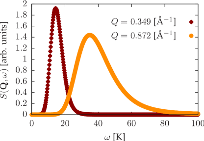
Figure 1: (Color online) Example of two reconstructed spectra at different wave-vectors along the $\Gamma A$ direction at the melting density $\rho_{1}$.

III Results

In this Section we present the results of our QMC simulations for both the phonon dispersion energies and the higher wave-vectors response of the solid.

III.1 Long wave-length excitations

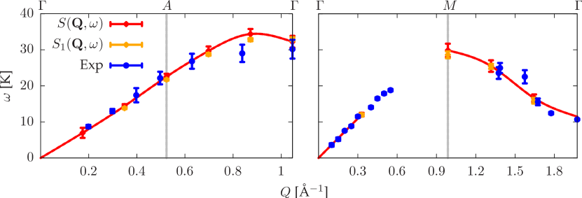
Figure 2: (Color online) Longitudinal phonon energies at the melting density $\rho_{1}$ extracted from $S(\mathbf{Q},\omega)$ and $S_{1}(\mathbf{Q},\omega)$, $\Gamma A$ and $\Gamma M$ directions (resp. left and right panel). The limit of the FBZ is indicated by a vertical grey line. Experimental data from Minkiewicz et al., 1968 and Minkiewicz et al., 1973. Frequencies calculated at discrete wave-vectors are interpolated by cubic splines as a guide to the eye.

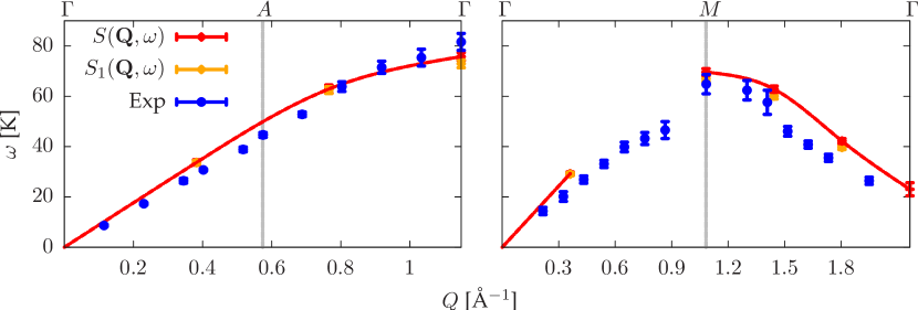
Figure 3: (Color online) Longitudinal phonon energies at the density $\rho_{2}=0.037\,[{\text{\r{A}}}^{-3}]$ extracted from $S(\mathbf{Q},\omega)$ and $S_{1}(\mathbf{Q},\omega)$, $\Gamma A$ and $\Gamma M$ directions (resp. left and right panel). The limit of the FBZ is indicated by a vertical grey line. Experimental data from Reese et al., 1971. Frequencies calculated at discrete wave-vectors are interpolated by cubic splines as a guide to the eye.

Longitudinal modes

The excitation energies of longitudinal vibrations can be straightforwardly obtained from the dynamic structure factor $S(\mathbf{Q},\omega)$, when available. In a lattice with a basis, such as hcp ${}^{4}\mathrm{He}$, multiple branches (acoustic and optic) exist at each point of the FBZ. Although for a generic wave-vector all the branches contribute to $S(\mathbf{Q},\omega)$, it often happens that—because of the explicit dependence of the inelastic structure factor 5 on both the wave-vector and the branch index—along high-symmetry directions different branches dominate (and in practice are only visible) at different values of the wave-vector. As a consequence, there are regions of the reciprocal space in which the acoustic modes dominate while the optical modes are suppressed and vice-versa. To figure out the relative weights of the branches, the inelastic structure factor can be calculated in a number of (approximate) ways, as in Ref. Schmunk et al., 1962 for beryllium, another hcp solid. By virtue of the strongly geometrical nature of $g^{2}(\mathbf{Q}|j)$, it is sufficient to look at one of these approximate calculations performed for the hcp geometry to realize that, with few exceptions, the relative weights do generally suppress one mode and privilege the other. Our results substantially confirm this picture, the calculated spectral functions being generally dominated by a single peak. Reconstructing a complete picture of the phonon dispersions thus require sampling the dynamic structure factor outside the FBZ.

We have calculated the phonon energies at the melting density $\rho_{1}=0.028\,[{\text{\AA}}^{-3}]$—in a regime of strong quantum fluctuations signaled by a considerable Lindemann’s ratio—and at the density $\rho_{2}=0.037\,[{\text{\AA}}^{-3}]$, where the quantum fluctuations are less pronounced. Results are shown in Figures 2 and 3 using an extended-zone scheme reminiscent of the way the optic and acoustic modes are measured in the lab. The phonon energies extracted by $S(\mathbf{Q},\omega)$ are compared to experimental data. The phonon energies resulting from an analysis of the one-phonon contribution to the dynamic structure factor are also shown for comparison.

The main findings that emerge from the calculations of the longitudinal modes are the following:

1. The overall agreement between the calculated and measured peak energies is good. The estimated errors come from the intrinsic width of the peaks of the dynamic structure factor, which is larger for optic than for acoustic phonon. This feature is present in both the theoretical and experimental spectra, although in the former the width is enhanced by the numerical difficulties in performing inverse Laplace transforms.

2. The discrepancy between the frequencies estimated in the one-phonon approximation and from the full dynamic structure factor is generally small. Multiphonon processes have clearly the effect of broadening the spectrum—particularly for large wave vectors—but they hardly affect the peaks’ positions.

3. In the $\Gamma M$ direction at the melting density $\rho_{1}$, we obtain a substantial improvement over SCP results.Gillis et al. (1968) We are thus able to separate the optic from the acoustic branches, which appear as distinct peaks in the dynamic structure factor. We also obtain a significant improvement over previous variational QMC results;Galli and Reatto (2003) besides, in Ref. Galli and Reatto, 2003 optical branches are calculated only in the $\Gamma A$ direction.

4. For the higher density $\rho_{2}$ we observe a stronger discrepancy between theoretical and experimental data, particularly in the $\Gamma M$ direction, possibly due to the pair potential adopted here.Moroni et al. (2000/03/20/)

Transverse modes

The direct evaluation of transverse phonon modes from the dynamic structure factor is hindered by the $\mathbf{Q}\cdot\bm{\epsilon}(\mathbf{q}|j)$ term appearing in its expression (Eqs. 4 and 5) that selects longitudinal modes. At least two strategies can be deployed to circumvent this problem. The most immediate solution consists in considering the peaks in the Fourier transform of the transverse counterpart of the one-phonon contribution to the dynamic structure factor:Sorkin et al. (2005)

$$S_{1\perp}(\mathbf{Q},t)\propto\left\langle\sum_{l,m}u_{\perp,l}(t)u_{\perp,m}(0)e^{i\mathbf{Q}\cdot\left(\mathbf{R}_{l}-\mathbf{R}_{m}\right)}\right\rangle,$$ (13)

where $u_{\perp,}$ is the transverse component of the atomic displacement from equilibrium. Although legitimate in principle, this approach is limited to the weak anharmonic regime and only gives access to the positions of the peaks, not to their intensities. A better approach, which in principle also gives access to peaks intensities, is to mimic closely the experimental practice and calculate the dynamic structure factor at wave-vectors $\mathbf{Q}=\mathbf{G}+\mathbf{q}$ such that $\mathbf{q}$ is arbitrarily quasi-perpendicular to $\mathbf{Q}$, so that a lattice vibration polarized parallel to $\mathbf{Q}$ is actually quasi-transverse:Mazzi et al. (2006) this is always possible, just choosing a large enough $\mathbf{G}$, i.e. looking at wave-vectors in the second, third, or successive Brillouin zones. In such a geometry transverse phonon energies at high-symmetry wave-vectors in the FBZ can be estimated from the peaks in the dynamic structure factor. In order to achieve a close comparison between our results and experimental data, our simulations at the melting density have been performed along the same quasi-transverse wave-vector directions as used in Ref. Minkiewicz et al., 1968.

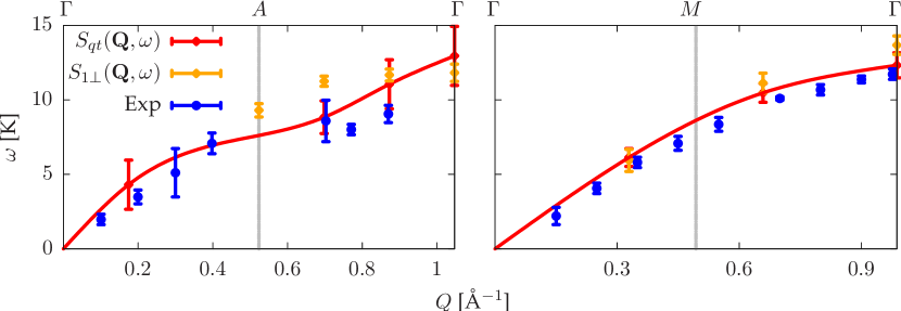
Figure 4: (Color online) Transverse phonon energies at the melting density $\rho_{1}$ extracted from the quasi-transverse geometry of $S(\mathbf{Q},\omega)$ and from the transverse components of $S_{1}(\mathbf{Q},\omega)$, $\Gamma A$ direction and $T_{\parallel}$ branch of the $\Gamma M$ direction (resp. left and right panel). The limit of the FBZ is indicated by a vertical grey line. Experimental data from Minkiewicz et al., 1968 and Minkiewicz et al., 1973. Frequencies calculated at discrete wave-vectors are interpolated by cubic splines as a guide to the eye.

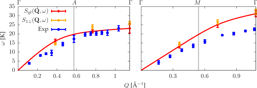
Figure 5: (Color online) Transverse phonon energies at the density $\rho_{2}=0.037\,[{\text{\r{A}}}^{-3}]$ extracted from the quasi-transverse geometry of $S(\mathbf{Q},\omega)$ and from the transverse components of $S_{1}(\mathbf{Q},\omega)$, $\Gamma A$ direction and $T_{\parallel}$ branch of the $\Gamma M$ direction (resp. left and right panel). The limit of the FBZ is indicated by a vertical grey line. Experimental data from Reese et al., 1971. Frequencies calculated at discrete wave-vectors are interpolated by cubic splines as a guide to the eye.

The transverse phonon energies thus obtained are presented in Figures 4 and 5, in an extended zone scheme.

The main findings that emerge from the calculations of the transverse modes closely parallel the results obtained in the longitudinal case:

1. The overall agreement with the experimental data is good.

2. The discrepancy between the energy obtained from the full dynamic form factor and from its one-phonon component is small. Energies from the full form factor tend to be more noisy than in the longitudinal case, possibly due to larger multi-phonon effects related to the large wave-vector involved in the quasi-transverse geometry.

3. We find a substantial improvement over the SCP results, particularly in the $\Gamma M$ direction, whilst there are no QMC results to compare with.

4. We find a systematic degradation of the agreement with experimental results for increasing density, especially for the direction $\Gamma M$ of Figure 5.

III.2 Intermediate wave-length excitations

Recent claims that solid ⁴He may display a supersolid behavior closely related to superfluidity in the liquid phase have prompted a revived interest in the experimental investigation of density excitations at intermediate wave-length, from which valuable information on the atomic momentum distribution can be extracted.Diallo et al. (2007) This experimental effort relies on the accurate determination of corrections to the Impulse Approximation (Eq. 9), a task which is facilitated in the large-momentum regime.Glyde (1994/09/01/)

Apart from the issues of off-diagonal long-range order and Bose-Einstein condensation in solid ⁴He, the role of atomic interference—as emerging from the additive corrections to the bare Impulse Approximation—has not yet been the subject of detailed theoretical investigations. To our knowledge, the best quantitative account of the response of solid helium is limited to the regions of small and very large wave-vectors.Glyde (1985) Nonetheless in the intermediate region where the long-wavelength spectra of both the liquid and the solid merge into the large-momentum regime of nearly free-particle recoil, no ab initio results have been reported so far.

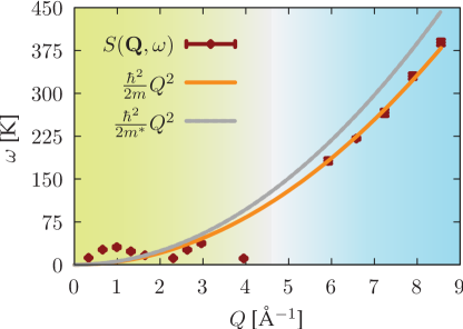
Figure 6: (Color online) Longitudinal excitations along the $\Gamma M$ direction at the density $\rho_{1}$. The solid line is the fitted free-particle dispersion of a quasi-particle with effective mass $m*$, while the grey line is the free-particle dispersion of atomic Helium. The two different background colors ideally separate the phonon region from the intermediate region of wave-vectors.

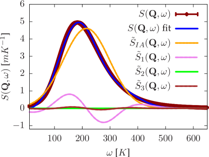
Figure 7: (Color online) Analysis of the dynamic structure factor into the Impulse Approximation and its additive corrections at the wave-vector $Q=5.92\,\text{\AA}^{-1}$ along the $\Gamma M$ direction.

Our QMC methodology, instead, allows us to provide an accurate description of this regime as well, showing evidence of a phonon-like residual coherence, not dissimilar to what is found in the superfluid phase.Martel et al. (1976/05/01/) We have concentrated our attention to wave-vectors roughly ranging from $5\,\text{\AA}^{-1}$ to $10\,\text{\AA}^{-1}$ between the phonon and the purely single particle regimes. The transition between these two regions can be clearly seen looking at the dispersion of the peaks of the dynamic structure factor, as a function of the excitation wave-vector. In Figure 6 the longitudinal excitation energies of the crystal at the melting density $\rho_{1}$ are shown. In the phonon-like regime (on the left of the figure with a yellowish background) we observe a periodic dispersion with soft modes corresponding to reciprocal-lattice vectors; for larger wave-vectors (on the right with a bluish background) we observe a free-particle parabolic dispersion, corresponding to an effective mass which is slightly higher than the bare Helium mass, being $M*\simeq 1.27\,M$.

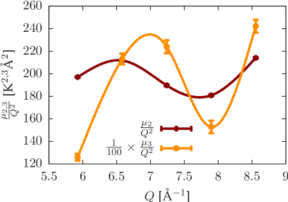
Figure 8: (Color online) Coherent oscillations of the cumulants $\mu_{2}$ and $\mu_{3}$ appearing in the additive corrections to the Impulse Approximation. Cumulants calculated at discrete wave-vectors are interpolated by cubic splines as a guide to the eye.

In order to characterize the density excitations of ${}^{4}\mathrm{He}$ in this region of momenta, we have analyzed the dynamic structure factor in terms of a cumulant expansion, Eq. (9), thus extending the scope of previous theoretical results, Glyde (1985) which were essentially unable to predict the response of the solid in this intermediate regime. In Figure 7 the calculated dynamic structure factor at the melting density $\rho_{1}$ is shown along with its decomposition in terms of the leading Impulse Approximation and its additive corrections of Eq. (10). The coefficients $\mu_{n}$ are taken as free parameters in the fitting procedure of the dynamic structure factor, much as it is done in the analysis of the experimental data.Glyde (1994/09/01/)

The bare Impulse Approximation of the dynamic structure factor overlooks quantum coherence effects in the density response functions, which are experimentally observedMartel et al. (1976/05/01/); Tanatar et al. (1987/12/01/) in superfluid ${}^{4}\mathrm{He}$. A better account of quantum coherence can be achieved including higher order corrections in the cumulant expansion of Eq. (9) whose non-vanishing contribution is in fact recognized in the fitting of our reconstructed spectra, Figure 7. The presence of quantum coherence between Helium atoms in the solid is further appreciated upon looking for deviations from the incoherent approximation of Eq. (6). A cumulant expansion of the incoherent dynamic structure factor can be carried out, and it is known Glyde (1994) that the cumulants of such an expansion $\mu_{2}^{\textit{inc}}$ and $\mu_{3}^{\textit{inc}}$ increase monotonically as $Q^{2}$ whereas $\mu_{4}^{\textit{inc}}$ and $\mu_{5}^{\textit{inc}}$ increase monotonically as $Q^{4}$. Characteristic $Q-$dependent oscillations in the ratios $\mu_{2,3}/Q^{2}$ and $\mu_{4,5}/Q^{4}$ can be therefore exploited to infer deviations from the purely incoherent response. Such oscillations have been observed in the superfluid phaseMartel et al. (1976/05/01/) and theoretically justified within a T-matrix approximation of the He-He atom scattering.Tanatar et al. (1987/12/01/) A similar behavior has also been recently observed in solid ${}^{4}\mathrm{He}$,Diallo et al. (2004) although no satisfactory ab-initio theoretical description exists yet. The cumulant dissection of the spectral properties extracted from our QMC simulations is a natural tool to examine the relics of quantum coherence in the intermediate wave-vector region, which closely parallels the experimental analysis. In Figure 8 we show the $Q-$dependent oscillations in the ratios $\mu_{2}/Q^{2}$ and $\mu_{3}/Q^{2}$ as found in our analysis of the dynamic structure factor, which are a quite clear manifestation of the residual coherence in the dynamics of solid helium in this intermediate region. The quantitative aspects of this analysis may be influenced by the quality of the Maximum Entropy reconstruction of the spectrum. However, the shift of the peak position with respect to the free particle recoil frequency should be reliable information, as suggested by the good agreement of the calculated and measured phonon dispersions previously shown.

IV Concluding remarks

In this work we have demonstrated and successfully applied a complete scheme to study the lattice dynamics of crystalline ⁴He at zero temperature. Although the stochastic nature of QMC methods limits us to explore the quantum imaginary time dynamics, we have shown that quantitative accuracy can be nonetheless achieved. One of the most appealing features of our analysis is the possibility to directly parallel the experimental investigation based on neutron scattering. The study of the full dynamic structure factor has allowed us to describe both the phonon and the intermediate wave-length regions of excitations.

At lower density, where the quantum fluctuations substantially affect the dynamics, we have obtained satisfactory results for the phonon energies, whereas approximate quasi-harmonic theories have shown difficulties in the accurate determination of the vibrational dispersions. An interesting point deserving more research is the effect of the adopted pair-potential on the calculated phonon branches. Our study suggests a degradation of the agreement to experimental data at higher density which could probably be alleviated upon the inclusion of higher than two body terms in the interatomic potential.

In the intermediate regime of wave-vectors, where the density excitations are better understood in terms of corrections to the small wave-length behaviour, we have shown that residual coherence in the quasi-particle excitations is present as in superfluid helium. Altough much of the theoretical and experimental efforts on the merging between the phonon and the single particle regimes have concentrated on the archetypal quantum solid –⁴He– we believe that an extension of such an analysis to other quantum solids such as ³He or molecular hydrogens H₂ would surely be worthwhile.