Transport Phase Diagram of Homogeneously Disordered Superconducting Thin Films

Abstract

We have constructed a phase diagram in temperature-magnetic field-disorder space for homogeneously disordered superconducting tantalum thin films. Phases are phenomenologically identified by the nonlinear transport characteristics that are unique in each phase. The resulting phase diagram shows that a direct superconductor-insulator transition is prohibited at any disorder because the superconducting phase is completely surrounded by the intervening metallic phase.

In two-dimensions (2D), a true superconducting state with zero electrical resistance is believed to exist only at zero temperature (T = 0). Increasing disorder in the system or applying magnetic fields (B) can disrupt the superconductivity, and eventually renders the system to an insulating state Finkelshtein (1987); Larkin (1999); Fisher (1990); Fisher et al. (1990). The transition between these two states in disordered films, however, is shrouded in mystery. While conventional theories, in either fermionic Finkelshtein (1987); Larkin (1999) or bosonic picture Larkin (1999); Fisher (1990); Fisher et al. (1990), expect a direct superconductor-to-insulator transition, a mysterious metallic phase intervening the two phases is reported, notably in Ta Seo et al. (2006); Qin et al. (2006); Vicente et al. (2006), MoGe Mason and Kapitulnik (2002); Ephron et al. (1996), and NbSi Aubin et al. (2006) films. The metallic state is usually identified by a drop in resistance followed by saturation to a finite value as $T\rightarrow 0$ that is much smaller than the normal state resistance ($\rho_{n}$). The metallic state is also known to exhibit a nonlinear transport with $d^{2}V/dI^{2}>0$ Seo et al. (2006); Qin et al. (2006); Vicente et al. (2006). This metallic nonlinear transport accompanies an extraordinarily long relaxation time, up to several seconds, and is demonstrated to arise from an intrinsic origin rather than to be a simple reflection of T-dependent resistivity via the combined effect of electron’s failure to cool and the Joule heating Seo et al. (2006). Three competing paradigms have been proposed to account for the emergence of the intervening metallic phase. The quantum vortex picture Galitski et al. (2005) describes the metallic phase as a Fermi-liquid of interacting vortices (vortex metal), the percolation paradigm Shimshoni et al. (1998); Ghosal et al. (2001); Dubi et al. (2006); Spivak et al. (2008) describes the films as consisting of superconducting and normal puddles, and the phase glass model Dalidovich and Phillips (2002); Wu and Phillips (2006) attributes the metallic transport to the coupling of the bosonic degrees of freedom to the excitations of the glassy phase.

So far, most of the experimental studies on the unexpected metallic phase are carried out in the lowest accessible temperatures. This is in part because the studies are more focused on the zero temperature ground state, and in part because of the lack of established experimental probes to characterize the metallic transport at elevated temperatures. In this Letter, we adopt nonlinear transport characteristics to identify the metallic phase and map the phase boundaries in the temperature-magnetic field plane. By combining such results from several films with different thicknesses representing different degree of disorder, we construct a 3D phase diagram in temperature-magnetic field-disorder space. The resulting phase diagram, which includes four different transport regimes, the superconducting, the metallic, the insulating, and the high temperature normal conducting phase, reveals two important features: 1) the superconducting phase is completely surrounded by the metallic phase prohibiting a direct superconductor-to-insulator transition at any disorder, and 2) the metallic phase appears even at zero field finite temperatures where the onset of superconductivity is usually understood in the framework of Kosterlitz-Thouless theory. In the rest of the paper, we describe how the phase boundaries are mapped and discuss the significance and implications of the resulting phase diagram.

Table 1: List of sample parameters: nominal film thickness t, normal state sheet resistance $\rho_{n}$ at 4.2 K, and the observed phases in each sample (S for superconducting phase, M for the metallic phase, I for the insulating phase, and N for the normal conducting phase). For samples exhibiting the superconducting phase, we list mean field $T_{c}$ at B = 0, the critical magnetic field $B_{c}$ as defined by the field at which the resistance reaches 90% of the high field saturation value, and the correlation length calculated from $\xi=\sqrt{\Phi_{0}/2\pi B_{c}}$ where $\Phi_{0}$ is the flux quantum.

Films	Batch	t(nm)	$\rho_{n}$(k$\Omega/\square$)	phase	$T_{c}$(K)	$B_{c}$(T)	$\xi$(nm)
Ta 1	1	5.6	1.42	S,M,I,N	0.65	0.82	20
Ta 2	2	4.1	2.28	S,M,I,N	0.26	0.33	32
Ta 3	3	2.5	3.04	M,I,N
Ta 4	3	2.4	3.34	M,I,N
Ta 5	3	2.3	3.54	M,I,N
Ta 6	3	2.2	3.88	M,I,N
Ta 7	3	2.1	4.20	I,N
Ta 8	3	2.0	4.98	I,N
Ta 9	3	1.0	6.20	I,N
Ta 10	4	2.5	6.24	I,N
Ta 11	5	2.5	8.00	I,N

The results reported in this Letter are from dozens of Ta films of which sheet resistances at T = 4.2 K range from 0.07 - 700 k$\Omega/\square$. Parameters of 11 samples whose data are shown in this paper are summarized in Table I. The Ta films are dc sputter deposited on Si substrate after baking the chamber at $\sim 110^{\circ}$C for several days reaching a base pressure below $10^{-8}$ Torr. Sample deposition rate was $\sim$ 0.05 nm/s with an Ar pressure of $\sim$ 4 mTorr. Prior to the deposition the chamber and Ta source were cleaned by a pre-sputtering process. Using a rotatable substrate holder, up to 12 films, each with a different thickness, can be grown without breaking the vacuum. Although there are noticeable batch to batch variations, the degree of disorder (evidence by the value of $\rho_{n}$) for films of the same batch increases monotonically with decreasing the nominal film thickness. All the samples were patterned into a Hall bar geometry (1 mm wide and 5 mm long) for four point measurements using a shadow mask. Ta films prepared this way are known to be structurally amorphous and homogeneously disordered Qin et al. (2006).

Shown in Fig.1(a) is a typical example of the T-dependence of resistance for a sample that undergoes a B-tuned superconductor-metal-insulator transition at the lowest temperature. At zero field (the bottom trace), the resistance at the lowest temperature is “immeasurably” small and is in the superconducting phase, the traces shown as thin solid lines correspond to the metallic phase, and for the top two traces (dashed lines) the sign of $d\rho/dT$ is always negative which is usually taken as an insulating signature.

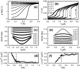
Figure 1: (a) Sheet resistance vs. T for Ta 2 at various magnetic fields in the range 0 – 0.5 T. (b) I-V curves of Ta 1 at T = 0.1 K at the indicated magnetic fields. Filled (open) circles are for current increasing (decreasing) branch. The solid lines are to indicate the electronic instabilities, and the arrows show the direction of the change. (c) dV/dI vs. I of Ta 1 at B = 0.6 T at the indicated temperatures. The solid lines are the fit to the quadratic function. (d) The quadratic coefficients obtained from the fitting are plotted against temperature for Ta 1. The solid lines are a guide to an eye, and the dashed line corresponds to the metal-normal conductor phase boundary. (e) dV/dI vs. I for Ta 2 at B = 2.0 T at the indicated temperatures. Solid lines are fit to the quadratic function. (f) Quadratic coefficients vs. T for sample Ta 2. The dashed line corresponds to the insulator-normal conductor boundary.

We first discuss the phase identification at the lowest temperature by the nonlinear transport characteristics that are unique in each phase. As reported earlier Seo et al. (2006); Qin et al. (2006), the superconducting phase exhibits a hysteretic I-V consisting of two electronic instabilities that appear as discontinuous voltage jumps occurring at different bias currents depending on whether the bias current is increasing or decreasing. Examples are shown in Fig.1(b). It is important to point out that 1) with approaching the instability the electronic relaxation time becomes increasingly longer, up to several seconds, and 2) the instabilities of the same characteristics are observed on films with normal state sheet resistances well below 100 $\Omega$. It has been already demonstrated Seo et al. (2006) that the instabilities are not due to electron’s self-heating. Instead, the above two observations are consistent with the picture that the instabilities correspond to the vortex pinning-depinning phenomena arising from the competition between Lorentz driving force on the vortices and pinning force due to disorder Paltiel et al. (2002). In this vortex picture all the vortices are expected to be pinned at zero temperature, which implies a realization of zero resistance state, or superconducting state, at zero temperature. With this reasoning, we judge the samples exhibiting hysteretic I-V’s to be in their superconducting phase. With increasing B the hysteresis systematically evolves into a smooth and reversible curve characterized by $d^{2}V/dI^{2}>0$ as the system is driven into the metallic phase. With further increasing B, eventually the system becomes an insulator with $d\rho/dT<0$, where $d^{2}V/dI^{2}$ is always negative. The origins of the nonlinear transport in the metallic and the insulating phase are not known. The metallic nonlinear transport might be caused by current-induced depinning of vortices as suggested by the accompanying extraordinarily long relaxation time, and the insulating nonlinear transport by a similar effect of current on localized Cooper pairs. Nevertheless, we take these nonlinear transport characteristics as a phenomenological indicator to distinguish the phases.

The phase boundaries are mapped by following the evolution of the nonlinear transport with changing T or B. The superconductor-metal boundary is determined as the temperature or field at which the hysteresis in I-V curve first disappears. Shown in Fig.1(b) is an example of B-driven evolution of the hysteretic I-V in the superconducting phase. With increasing B, the hysteresis becomes progressively smaller and disappears at B $\approx$ 0.13 T, which we identify as a superconductor-metal boundary. The T-driven evolution is similar as reported in Ref. Seo et al. (2006).

In the metallic phase, it is convenient to analyze the nonlinear transport in terms of differential resistance. As shown in Fig.1(c), the nonlinearity progressively becomes weaker with increasing temperature and eventually the transport becomes linear. The linear transport at high temperatures is natural because at sufficiently high temperatures the system should be in the normal conducting state where the transport is linear. In order to quantitatively identify the phase boundary, we fit the dV/dI vs. I trace to a quadratic function $dV/dI=cI^{2}+\rho_{0}$, where c is the quadratic coefficient and $\rho_{0}$ is the sample s sheet resistance in the zero bias current limit. When the nonlinearity is relatively weak, the fitting is quite reasonable as shown by the solid curves for the top four traces in Fig.1(c). In Fig.1(d) the quadratic coefficients obtained from the least squared error fittings are plotted as a function of temperature. This plot shows that the behavior of the quadratic coefficients changes abruptly at a well defined temperature: At low temperatures (below the dashed line) the coefficients are rather strongly temperature dependent. At high temperatures (above the dashed line) the coefficients are almost temperature independent and the values are close to zero, implying the transport is practically linear. We identify the boundary, the dashed line in Fig.1(d), as the phase boundary separating the metallic phase and the high temperature normal conducting phase.

Figure 1(e) shows a similar evolution of the nonlinear transport in the insulating phase. The same quadratic function is used to fit the data. When the nonlinearity is relatively weak the fitting is very reasonable [solid lines in Fig.1(e)]. Again, as shown in Fig.1(f), there is a well defined temperature across which the behavior of the quadratic coefficients is distinctly different. We identify the low temperature regime (below the dashed line) where the T-dependence of the coefficients is relatively strong as the insulating phase, and the high temperature regime where the coefficients are almost T-independent and almost zero as the high temperature normal conducting phase.

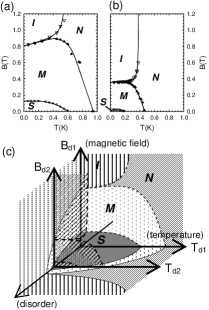
Figure 2: (a) Phase diagram of Ta 1 in the B-T plane. Symbols are experimental data and solid lines are to guide an eye. The superconducting phase is marked by S, the metallic phase by M, the insulating phase by I, and the normal conducting phase by N. (b) Phase diagram of Ta 2, which is more disordered than Ta 1. (c) The topology of the 3D phase diagram in T-B-disorder space is shown. Disorder is represented by the normal state sheet resistance and the axis only indicates the direction of increasing disorder. The illustrated phase diagram does not include the clean limit. The diagram shown in (a) for Ta 1 can be considered as a cross-sectional view on the plane of $T_{d1}-B_{d1}$, and the diagram for Ta 2 can be considered as a cross-sectional view on the plane of $T_{d2}-B_{d2}$.

The phase boundaries determined as described above are shown in Fig.2(a) and (b) for two samples, Ta 1 and Ta 2. Both samples are relatively weakly disordered and all four phases appear. The superconducting phase is marked by S, the metallic phase by M, the insulating phase by I, and the high temperature normal conducting phase by N. As represented by their normal state sheet resistances Ta 2 is more disordered than Ta 1. The results from these two samples capture the main feature that both the superconducting and the metallic phase shrink to lower temperature and lower field regime with increasing disorder and the insulating phase extends to lower fields. This tendency was clear in about a dozen other samples we investigated, although their data are not shown in this paper. This tendency is depicted in the 3D phase diagram in the T-B-disorder space in Fig.2(c), where the phase diagram of Ta 1 corresponds to a cross-sectional view in the plane of $T_{d1}-B_{d1}$ and the phase diagram of Ta 2 corresponds to a cross-sectional view at a higher disorder, $T_{d2}-B_{d2}$ plane.

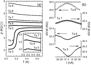
Figure 3: (a) T-dependence of resistance of samples Ta 3 – 9 at B = 0 is shown. All these samples are grown in a single batch. (inset) A blow-up view of resistance behavior at low temperatures for samples Ta 5 – 7. (b) Differential resistance (dV/dI) vs. I for samples Ta 5 – 8. The arrows indicate the corresponding scale for each trace.

With further increasing disorder, we reach the regime where the superconducting phase no longer exists even at T = 0 and B = 0. This disorder regime appears as a gap between the superconducting and insulating phase along the disorder axis in Fig.2(c). In this disorder regime, the metallic phase occupies the low T and low B region in the phase diagram. Examples of such a metallic behavior at B = 0 is shown in Fig.3(a) as thick solid lines. The bottom two traces exhibit a rather steep drop in resistance followed by saturation to a finite value as $T\rightarrow 0$. Samples Ta 5 and Ta 6 show only a weak T-dependence. However, as shown in the inset their slopes are positive at low temperatures and their nonlinear transport is characterized by $d^{2}V/dI^{2}>0$ [filled circles in Fig.3(b)]. We emphasize that the metallic behaviors of these samples observed under B = 0 are indistinguishable from the B-induced metallic behaviors of samples of weak disorder such as Ta 1 or Ta 2. For even more disordered samples (samples Ta 7 – 9), $d\rho/dT$ is always negative with nonlinear transport of $d^{2}V/dI^{2}<0$ [open circles in Fig.3(b)], which are the insulating characteristics. In this high disorder regime where only the insulating phase appears at low temperatures, the boundary of the insulating phase grows to a higher temperature with increasing disorder. This tendency is shown in Fig.4(a) – (c).

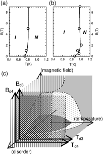
Figure 4: (a) Phase diagram of Ta 10 in the T-B plane. Insulating phase is marked by I and the normal conducting phase by N. Solid lines are to guide an eye. (b) Phase diagram of Ta 11 in the T-B plane. Ta 11 is more disordered than Ta 10 by the measure of $\rho_{n}$. (c) The same 3D phase diagram shown in Fig.2(c), but includes the corresponding cross-sectional views for Ta 10 ($T_{d3}-B_{d3}$ plane) and Ta 11 ($T_{d4}-B_{d4}$ plane). The hatched area in the $T_{d3}-B_{d3}$ ($T_{d4}-B_{d4}$) plane corresponds to the insulating phase of Ta 10 (Ta 11).

With the presence of the B = 0 metallic phase tuned by disorder, the superconducting phase is completely surrounded by the metallic phase prohibiting a direct superconductor-insulator transition at any disorder. This is a fundamental difference from the phase diagram proposed earlier Steiner et al. (2008). Authors of Ref. Steiner et al. (2008), based on their scaling analysis, have proposed a phase diagram where the metallic phase can exist only in weak disorder regime under finite magnetic fields. In their phase diagram, a direct superconductor-insulator transition occurs in a relatively high disorder regime. While this discrepancy between the two phase diagrams is a puzzle that needs to be solved, we note that all the samples interpreted to exhibit a direct superconductor-insulator transition in Ref. Steiner et al. (2008) are InO material systems which are known to have a wide resistive superconducting transition Shahar . Typically, the width of the transition in InO ($\Delta T_{c}/T_{c}$), with $\Delta T_{c}$ being the temperature interval corresponding to the resistance change from 90% to 10% of normal state resistance at B = 0, is larger than that observed in Ta systems by several times or more. The width of the resistive transition, $\Delta T_{c}/T_{c}$, can be a measure of disorder at a length scale longer than the superconducting coherence length. However, what role this long length scale disorder plays is not clear at present.

Finally, we turn to the discussion on the metallic phase appearing in the B = 0 finite temperature region [for example, the metallic phase along the temperature-axis in Fig.2(c)]. One might argue that the nonlinear transport with $d^{2}V/dI^{2}>0$ of samples in this metallic phase could come from the Kosterlitz-Thouless (KT) mechanism Kosterlitz and Thouless (1973). The KT theory has been the framework to understand the onset of superconductivity in 2D at a finite temperature at B = 0. In this picture, the superconducting transition is described as a thermodynamic instability of vortex-antivortex pairs. The transport in the superconducting phase is expected to be nonlinear in a power law fashion, $V\propto I^{\alpha}$ with $\alpha>3$, due to the current-induced vortex pair dissociations Halperin and Nelson (1979). It has been argued Medvedyeva et al. (2000) that in a real system a strong finite size effect can induce free vortices altering the power law. The resulting nonlinear transport obtained in a numerical simulation Medvedyeva et al. (2000) closely resembles what is observed in our samples in their metallic phase. However, as reported earlier Seo et al. (2006); Qin et al. (2006), we observe two transport properties that cannot be reconciled with the KT picture: One is the extraordinarily long relaxation time, up to several seconds, and the other is the development of electronic instabilities appearing as a sharp hysteresis in I-V curves at low temperatures. These observations indicate that the metallic nonlinear transport in the B = 0 and finite temperature region is unlikely related to the KT mechanism, and raise the possibility that the KT transition might have been pre-emptied by a first order vortex pinning-depinning transition.

To summarize, we have mapped a phase diagram in T-B-disorder space for homogeneously disordered superconducting Ta films. The phase diagram includes four different phases: the superconducting phase identified by the presence of electronic instability possibly due to vortex pinning-depinning mechanism, the metallic phase by $d^{2}V/dI^{2}>0$, the insulating phase by $d^{2}V/dI^{2}<0$, and the normal conducting phase by $d^{2}V/dI^{2}=0$. The resulting phase diagram shows that the superconducting phase is completely surrounded by the intervening metallic phase prohibiting a direct superconductor-insulator transition at any disorder, and that the metallic phase extends to B = 0 finite temperature region.

The authors acknowledge fruitful discussions with G. Refael and H. Fertig. This work was supported by the NSF through Grant No. DMR-0239450.

References

- Finkelshtein (1987) A. Finkelshtein, JETP Lett. 45, 46 (1987).
- Larkin (1999) A. Larkin, Ann. Phys. 8, 785 (1999).
- Fisher (1990) M. P. A. Fisher, Phys. Rev. Lett. 65, 923 (1990).
- Fisher et al. (1990) M. P. A. Fisher, G. Grinstein, and S. M. Girvin, Phys. Rev. Lett. 64, 587 (1990).
- Seo et al. (2006) Y. Seo, Y. Qin, C. L. Vicente, K. S. Choi, and J. Yoon, Phys. Rev. Lett. 97, 057005 (2006).
- Qin et al. (2006) Y. Qin, C. L. Vicente, and J. Yoon, Phys. Rev. B 73, 100505(R) (2006).
- Vicente et al. (2006) C. L. Vicente, Y. Qin, and J. Yoon, Phys. Rev. B 74, 100507(R) (2006).
- Mason and Kapitulnik (2002) N. Mason and A. Kapitulnik, Phys. Rev. B 65, 220505(R) (2002).
- Ephron et al. (1996) D. Ephron, A. Yazdani, A. Kapitulnik, and M. R. Beasley, Phys. Rev. Lett. 76, 1529 (1996).
- Aubin et al. (2006) H. Aubin et al., Phys. Rev. B 73, 094521 (2006).
- Galitski et al. (2005) V. M. Galitski, G. Refael, M. P. A. Fisher, and T. Senthil, Phys. Rev. Lett 95, 077002 (2005).
- Shimshoni et al. (1998) E. Shimshoni, A. Auerbach, and A. Kapitulnik, Phys. Rev. Lett 80, 3352 (1998).
- Ghosal et al. (2001) A. Ghosal, M. Randeria, and N. Trivedi, Phys. Rev. B 65, 014501 (2001).
- Dubi et al. (2006) Y. Dubi, Y. Meir, and Y. Avishai, Phys. Rev. B 73, 054509 (2006).
- Spivak et al. (2008) B. Spivak, P. Oreto, and S. A. Kivelson, Phys. Rev. B 77, 214523 (2008).
- Dalidovich and Phillips (2002) D. Dalidovich and P. Phillips, Phys. Rev. Lett. 89, 027001 (2002).
- Wu and Phillips (2006) J. Wu and P. Phillips, Phys. Rev. B 73, 214507 (2006).
- Paltiel et al. (2002) Y. Paltiel et al., Phys. Rev. B 66, 060503(R) (2002).
- Steiner et al. (2008) M. A. Steiner, N. P. Breznay, and A. Kapitulnik, Phys. Rev. B 77, 212501 (2008).
- (20) D. Shahar, private communication.
- Kosterlitz and Thouless (1973) J. D. Kosterlitz and D. J. Thouless, J. Phys. C 6, 1181 (1973).
- Halperin and Nelson (1979) B. I. Halperin and D. R. Nelson, J. Low Temp. Phys. 36, 599 (1979).
- Medvedyeva et al. (2000) K. Medvedyeva, B. J. Kim, and P. Minnhagen, Phys. Rev. B 62, 14531 (2000).