The Evolution of Gas Clouds Falling
in the Magnetized Galactic Halo:
High Velocity Clouds (HVCs)
Originated in the Galactic Fountain

Abstract

In the Galactic fountain scenario, supernovae and/or stellar winds propel material into the Galactic halo. As the material cools, it condenses into clouds. By using FLASH three-dimensional magnetohydrodynamic simulations, we model and study the dynamical evolution of these gas clouds after they form and begin to fall toward the Galactic plane. In our simulations, we assume that the gas clouds form at a height of $z=5~{}\mbox{kpc}$ above the Galactic midplane, then begin to fall from rest. We investigate how the cloud’s evolution, dynamics, and interaction with the interstellar medium (ISM) are affected by the initial mass of the cloud. We find that clouds with sufficiently large initial densities ($n\geq 0.1~{}\mbox{H atoms}~{}\mbox{cm}^{-3}$) accelerate sufficiently and maintain sufficiently large column densities as to be observed and identified as high-velocity clouds (HVCs) even if the ISM is weakly magnetized ($1.3~{}\mu$G). However, the ISM can provide noticeable resistance to the motion of a low-density cloud ($n\leq 0.01~{}\mbox{H atoms}~{}\mbox{cm}^{-3}$) thus making it more probable that a low-density cloud will attain the speed of an intermediate-velocity cloud rather than the speed of an HVC. We also investigate the effects of various possible magnetic field configurations. As expected, the ISM’s resistance is greatest when the magnetic field is strong and perpendicular to the motion of the cloud. The trajectory of the cloud is guided by the magnetic field lines in cases where the magnetic field is oriented diagonal to the Galactic plane. The model cloud simulations show that the interactions between the cloud and the ISM can be understood via analogy to the shock tube problem which involves shock and rarefaction waves. We also discuss accelerated ambient gas, streamers of material ablated from the clouds, and the cloud’s evolution from a sphere-shaped to a disk- or cigar-shaped object.

1 Introduction

Neutral hydrogen (H I) clouds that have large local standard of rest velocities ($|V_{\mbox{LSR}}|\geq 90~{}\mbox{km}~{}\mbox{s}^{-1}$) were first discovered by Muller et al. (1963) and identified as high-velocity clouds (HVCs). For HVCs at high latitude, these velocities are incompatible with a simple model of the differential rotation of the Galaxy. Thus, a 40 yr long search for their origins began. The three leading models propose that HVCs originate from: the Galactic fountain; the infall of matter stripped from smaller galaxies that orbit the Milky Way; and the accretion of primordial gas left over from the epoch of galaxy formation. In the fountain scenario (Shapiro & Field 1976), material from the Galactic disk is pushed into the lower Galactic halo by superbubbles (made by a series of co-located supernovae in an OB cluster), radiatively cools, and then falls back to the Galactic disk due to the force of gravity. This model is capable of explaining both upward-moving and downward-moving HVCs, and intermediate-velocity clouds (IVCs) which are H I clouds with intermediate velocities ($40~{}\mbox{km}~{}\mbox{s}^{-1}\leq|V_{\mbox{LSR}}|\leq 90~{}\mbox{km}~{}\mbox{s}^{-1}$; Kuntz & Danly 1996). In the second model, gas is stripped from nearby galaxies. The Magellanic Stream (MS), which is associated with the Large Magellanic Cloud (LMC) and the Small Magellanic Cloud (SMC), is an example. In addition, there are more than a dozen dwarf galaxies within $100~{}\mbox{kpc}$ of the Milky Way (see Belokurov et al. (2007), and references therein). These dwarf galaxies may have been stripped of their gas during previous passages through the Milky Way as the Sagittarius Dwarf Galaxy is thought to have been (Putman et al. 2004). In the accretion scenario, some of the gas left over from the formation of the Galaxy is currently being accreted (Oort 1966). Blitz et al. (1999) developed this idea further, claiming that HVCs are material moving under the gravitational potential of the Local Group of galaxies. According to their model, nearby HVCs are falling onto the Galactic disk due to tidal instabilities, although fewer HVCs probably have intergalactic origins than Blitz et al. (1999) originally expected.

For any given HVC, the applicability of different models can be distinguished by the distance to the HVC and the HVC’s metallicity, but metallicity is widely believed to be the better discriminant. Clouds made by the Galactic fountain should be relatively near to the Galactic plane ($\leq 5~{}\mbox{kpc}$) and have substantial metallicities (comparable to the solar metallicity). Generally, the clouds that originated from extragalactic sources may be further away than clouds produced by the Galactic fountain, although it is possible that externally produced HVCs could eventually approach the Galactic plane after falling for a long time. For such HVCs, a measurement of their low metallicities would be needed in order to assign the primordial gas accretion model. For HVCs that are composed of gaseous material that was stripped off of the satellite galaxies orbiting the Milky Way, their metallicities should be strongly correlated with those of the satellite galaxies. Generally they should be intermediate between those of the Milky Way’s disk and those of intergalactic clouds.

According to the current measurements of distances and metallicities, not all HVCs have the same origin. For example, the metallicity of the MS is reported to be $\sim 0.25$ solar, which is consistent with the metallicity of the SMC and LMC (Lu et al. 1998; Gibson et al. 2000). This consistency together with the geometrical association of the MS with the SMC and LMC provides strong evidence that the MS material came from the SMC and LMC. The distance upper limit ($z<4$ kpc; Danly et al. 1993; Keenan et al. 1995) and solar-comparable metallicity ($\sim 0.8$ solar; Tufte et al. 1998; Wakker 2001) of Complex M put it in the list of those made by Galactic fountains. Complex C, which is one of the most extensively studied HVCs, is more likely to have an extragalactic origin because of its relatively low metallicity. The most recently measured metallicity and distance bracket are $\sim 0.13$ solar (Collins et al. 2007) and approximately between 4 and 11 kpc (Wakker et al. 2007; Thom et al. 2008), respectively. Primordial inter-galactic medium (IGM) gas is thought to have metallicities of $\leq 0.1$ solar (Davis et al. 1996), thus clouds formed from the IGM may have similarly low metallicities.

In this paper, we further examine clouds produced in the Galactic fountain. By using three-dimensional magnetohydrodynamic (MHD) simulations made with FLASH version 2.5 (Fryxell et al. 2000), we model and study the dynamical evolution of gas clouds that form in the Galactic fountain process and start to fall from rest. The goal of our simulations is to investigate whether these clouds could develop the characteristics of HVCs when they fall back toward the Galactic plane, specifically whether they could accelerate to the velocities of HVCs while retaining sufficiently large column densities to be observable. The initial clouds are assumed to form at the height $z=5~{}\mbox{kpc}$ above the Galactic midplane when the radiatively cooled gas condenses at the peak of the fountain process. The peak location at which the dense clouds form is not directly constrained by observations, but the hydrodynamic (HD) simulations of de Avillez (2000) suggest that $5$ kpc is within the reasonable height range. Besides, in order for a cloud to accelerate from rest to $|v|>90~{}\mbox{km}~{}\mbox{s}^{-1}$ under the Galaxy’s gravity, it must fall from a height of at least a few kiloparsec above the Galactic midplane. Note that the clouds in our simulations fall down directly toward an observer so that the observed velocities are the same as the vertical velocities. However, in the cases in which the cloud’s velocity vector is not parallel to the sight line to the observer, the observed velocity is smaller than the cloud’s real velocity.

Since the initial cloud falls through the Galactic halo, which is filled with a low density interstellar medium (ISM) as well as a magnetic field, its interaction with the ISM also affects the dynamical evolution of the cloud. Because the conditions of the Galactic halo and the initial cloud are not precisely constrained by the observations, we survey a large range of possible conditions. We pay special attention to the effects of both the strength and the orientation of the interstellar magnetic field. In order to determine the effects of magnetic field geometries, we consider three different magnetic field configurations in the Galactic halo: parallel, perpendicular, and $45\arcdeg$ with respect to the Galactic plane. Cases with no magnetic field are also performed and two initial cloud densities are examined.

Previous work demonstrated that HD and MHD simulations are well developed and useful tools for studying HVCs (Tenorio-Tagle et al. 1986, 1987; Santillán et al. 1999; Kudoh & Basu 2004). The two-dimensional HD simulations by Tenorio-Tagle et al. (1986, 1987) implied that very massive HVCs shocked and perturbed the Galactic disk. The two-dimensional HD simulations of Kudoh & Basu (2004) implied that HVC-galaxy interactions could explain unusual observed structures in our galaxy, such as the mushroom-shaped GW 123.4-1.5. Santillán et al. (1999) used the two-dimensional MHD simulations to examine the important role of the magnetic field. They found that magnetic field lines that are oriented perpendicular to the cloud’s motion became sufficiently stretched and compressed as to prevent HVCs from falling closer to the Galactic disk. In their simulations, the ISM is assumed to be isothermal and in hydrostatic equilibrium (HSE) in which the gravity is balanced by the gradients both in the thermal and magnetic pressures. Note that at the beginning of their simulations, the HVCs were already close to the Galactic plane and usually moving rapidly. This initial configuration is based upon the assumption that either HVCs had originated at large $z$-heights but did not interact significantly with the extended halo ISM or HVCs originated close to the Galactic plane. Our simulations are different from these cloud–disk interaction simulations because we simulate all three dimensions and because the primary goals of our simulations are to determine whether gas clouds that form in the Galactic fountain process could accelerate to HVC velocities and to determine how the interstellar magnetic field and initial cloud density affect the outcome.

This paper is organized as follows. The model parameters used in our simulations are summarized in Section 2. We will briefly describe the numerical methods used for our simulations in Section 3. The results of the simulations are presented in Section 4. We will discuss our results further and their connection to observations in Section 5. In Section 5, we will also show how the model geometries that we choose for the magnetic field in the Galactic halo can be related to realistic configurations in the context of the Galactic fountain model. Our conclusions are explained in Section 6.

2 Modeled Physical Processes and Parameters

The physical state of the ISM at the height of the Galactic halo is less well known than that of the ISM in the Galactic disk. Nonetheless, estimates have been made from a wide variety of observational evidence. In our simulations, we use the density and gravitational acceleration equations of Ferriere (1998) and assume that their functional forms can be extrapolated to large heights above the plane, i.e., $z\approx 5$ kpc. We ignore the molecular hydrogen density because most molecular clouds reside close to the Galactic plane. Figure 1 shows the hydrogen number density and gravitational acceleration profiles within the computational domain of our simulations.

The total weight per unit area of the gaseous material residing above the height, $z$, can be calculated from the density and acceleration profiles and is shown in Figure 1. In our calculation, we assume that the total weight per unit area of the ISM above $z=20~{}\mbox{kpc}$ is zero. We also assume that the ISM in the Galactic halo is in HSE, which allows us to calculate the gradient in the total pressure by setting it equal to the gradient in the weight per unit area (i.e., the gravitational force per volume). Generally, the total pressure is composed of three components; thermal, magnetic, and cosmic-ray pressure. In our simulations, we include only thermal and magnetic components because our primary interest is the dynamical effect of the magnetic field and because it is difficult to model the cosmic-ray pressure in the numerical simulations. However, in our simulations, the interstellar magnetic field strength does not vary with height. Thus, the gradient in the total pressure is entirely due to the gradient in the thermal pressure. Therefore, the ISM in our simulations is in HSE if the gradient in the weight per unit area is balanced by the gradient in the thermal pressure alone. Additionally, we assume that there is no constant offset between these two variables. Thus, we set the thermal pressure at height $z$, equal to the weight per unit area of the gaseous material above height $z$.

The thermal pressure, $p_{th}(z)$, at the height $z$ is given by $p_{th}(z)=n(z)~{}k_{B}~{}T(z)$, where $k_{B}$ is the Boltzmann’s constant and $n(z)$ and $T(z)$ are the total number of particles per unit volume and the temperature at the height $z$, respectively. The density of atomic nuclei is taken to be $110\%$ of the density of hydrogen because the helium abundance in the ISM is $10\%$ of the hydrogen abundance. In order to apply the MHD simulations, we also assume that both hydrogen and helium are fully ionized. As a result, the density of particles is $n(z)=2.3~{}n_{H}(z)$, where $n_{H}(z)$ is hydrogen number density from Ferriere (1998) that is shown in Figure 1. The temperature, $T(z)$, in Figure 1 is calculated from $p_{th}(z)$ and $n(z)$. Because $n(z)$ incorporates contributions from cold dense gas, warm moderately dense gas, and hot rarefied gas, $n(z)$ and $T(z)$ are phase-averaged quantities. Therefore, the temperature of the ISM used in our simulations is less than a million degrees Kelvin. We will discuss the effect of the ISM temperature after discussing our simulation results (see Section 5.4).

Given the current uncertainty about the magnetic field in the Galactic halo, we consider only simple cases, in which the strength of the magnetic field, $B$, is initially constant throughout the simulation domain. This allows us to choose different values of the constant magnetic field strength for different simulation models without violating the HSE condition. In order to analyze the effect of the magnetic field strength, we choose two different values for the magnetic pressure, $7.0\times 10^{-14}$ and $7.0\times 10^{-13}$ $\mbox{erg}~{}\mbox{cm}^{-3}$ which correspond to $B=$ $1.3$ and $4.2$ $\mu\mbox{G}$, respectively. These two values are consistent with the strength of the magnetic field in the lower halo. The two magnetic pressure values are plotted together with the total weight per unit area in Figure 1.

We consider three different configurations for the initial magnetic field orientation: parallel, perpendicular, and tilted at $45\arcdeg$ with respect to the Galactic plane. In the three-dimensional Cartesian coordinates of our simulations, where $x$ and $y$ axes are in the Galactic plane, we set up the “parallel magnetic field” to be parallel to the $z$-axis and the direction of the cloud’s motion ($B_{z}=\mbox{constant}$ and $B_{x}=B_{y}=0$). The “perpendicular magnetic field” is perpendicular to the $z$-axis and the direction of the cloud’s motion ($B_{y}=\mbox{constant}$ and $B_{x}=B_{z}=0$). In the case where the magnetic field is titled at $45\arcdeg$ we set it up along the $y$-$z$ plane ($B_{y}=B_{z}=\mbox{constant}$ and $B_{x}=0$). We also simulate cases with no magnetic field. In all, we present nine cases ( A1 and A2, which have no magnetic field, B1-B4, which have a magnetic field that is perpendicular to $\hat{z}$, C1 and C2, which have a magnetic field that is parallel to $\hat{z}$, and D, in which the magnetic field orientation is tilted). The model parameters for the ambient ISM, magnetic pressure, and orientation are summarized in Table 1.

In our simulations, a spherical gas cloud with a radius of $0.25~{}\mbox{kpc}$ falls down from rest through the ambient ISM. The center of the gas cloud is initially located at a height $z=5~{}\mbox{kpc}$. The cloud is homogeneous within the sphere and its hydrogen number density is either $0.01~{}\mbox{cm}^{-3}$ for a low-density cloud or $0.1~{}\mbox{cm}^{-3}$ for a high-density cloud. The corresponding cloud’s mass is approximately $2.26\times 10^{4}$ and $2.26\times 10^{5}~{}\mbox{M}_{\sun}$ for the low- and high-density cloud, respectively. For a sight line passing through the center of the cloud, the hydrogen column density is approximately $1.5\times 10^{19}$ and $1.5\times 10^{20}~{}\mbox{cm}^{-2}$, respectively, if the cloud’s radius is 0.25 kpc and the whole cloud is made of gas with hydrogen volume densities of $0.01$ and $0.1~{}\mbox{cm}^{-3}$, respectively. These column densities are common of observed HVCs. The $1.5\times 10^{19}$ case is near the center of the observed range in column densities, while $1.5\times 10^{20}~{}\mbox{cm}^{-2}$ is close to the largest observed HVC column density (Wakker 2001). The modeled cloud is initially in pressure equilibrium with the ambient ISM, that is, the thermal pressure of the cloud at the height $z$ is the same as that of the ambient ISM. Therefore, the initial temperature of the gas in the cloud varies with height, from about $5000$ to $7400$ K for the low-density cloud and from about $500$ to $740$ K for the high-density cloud. The magnetic field lines of the ambient ISM pass through the initial cloud without change in strength or orientation. The self-gravity of our model cloud can be ignored because it is much less than the Galactic gravity.

Because the primary goal of the our numerical study is to determine whether or not clouds made by the fountain process can gravitationally accelerate to HVC velocities, we must model gravity. Gravity also acts on the ambient gas, so to prevent it from collapsing, we assume that it is in HSE, as is frequently done in numerical studies of cloud–ISM interactions (Tenorio-Tagle et al. 1987; Santillán et al. 1999; Kudoh & Basu 2004). However, in order to maintain HSE, the background gas cannot be subject to net heating or cooling. For this reason, we disallow radiative cooling, radiative heating, and thermal conduction.

Although we do not include radiative cooling, external heat sources (aside from the cloud impact), or heat conduction, other authors have considered their effects. Cowie & McKee (1977) and McKee & Begelman (1990) analytically calculated the evaporation and condensation rates experienced by a cool, static cloud embedded in a hot (a few million degree) ambient gas due to thermal conduction and radiative cooling. Their analytic calculations showed that the cool static cloud evaporates even when the rate of heat conduction is saturated. Vieser & Hensler (2007a) tested these analytic results by numerical simulations of static clouds in a hot ambient medium, and their numerical simulations showed a new result; the clouds experience delayed evaporation or the ambient gas condenses onto the clouds when saturated heat conduction or radiative heating and cooling are considered. In the dynamical case, in which the cloud interacts with hot ($5\times 10^{6}$ K) streaming ambient gas (Vieser & Hensler 2007b), the evaporation of the cloud due to thermal conduction is even further delayed. Given their results, the clouds in our simulations should not be expected to evaporate easily if thermal conduction were allowed. In addition, the cloud–ISM temperature gradient in our simulations is $\sim~{}1/10$ of that in Vieser & Hensler (2007b), making the clouds that we examine even less likely to evaporate due to thermal conduction.

In dynamical situations, thermal conduction plays the role of a diffusion process. For this reason, it is sometimes ignored in cases in which there are more dominant diffusion processes. For example, de Avillez & Breitschwerdt (2007) found turbulent diffusion to be more significant than thermal conduction in their simulations. Slavin et al. (1993) also argued that turbulent mixing together with radiative cooling cools the gas more efficiently than thermal conduction. In our simulations, modeling the diffusion of heat in the region between the cloud and the shock front would have the effect of decreasing the thermal pressure gradient and therefore the resistance to the cloud’s downward motion. Its effect would be very small when the magnetic field is oriented perpendicular to the cloud’s motion because in this case the resisting force due to the magnetic pressure gradient is much larger than that due to the thermal pressure gradient. Note that in this case thermal conduction is reduced significantly because electrons that are responsible for thermal conduction are prevented from carrying the thermal energy across the magnetic field lines. In the other cases, those in which there is no magnetic field or the field lines are parallel to the cloud’s motion, we anticipate that the clouds would fall slightly faster if thermal conduction were modeled.

In our MHD simulations, the effect of turbulent mixing due to shear instabilities is reduced because the magnetic field suppresses the growth of shear instabilities (Mac Low et al. 1994; Jones et al. 1996). We expect that the inclusion of thermal conduction would further reduce turbulent mixing because Vieser & Hensler (2007b) found that thermal conduction suppresses the growth of shear instabilities when the cool cloud moves through hot gas.

3 Numerical Methods

We use the MHD module of FLASH version 2.5 (Fryxell et al. 2000) for our simulations. FLASH is an Eulerian grid-based code which was found to model cloud instabilities and fragmentation better than smoothed particle hydrodynamics (SPHs) codes (Agertz et al. 2007). The external gravity module in FLASH is used to deal with the Galaxy’s gravitational force on the Galactic halo. The non-magnetic simulations of Model A are performed with the MHD module by setting the initial magnetic field to zero.

FLASH uses a block-structured adaptive mesh refinement (AMR) technique implemented through PARAMESH (MacNeice et al. 2000). When AMR is used, only the “interesting” region within the computational domain is resolved better. It is resolved with smaller meshes than the other regions, thus saving computing time. In our simulations, we choose the density gradient as the refinement criterion. Because the density gradient is large in the vicinity of the cloud, this region is always modeled with high resolution during the simulation. The other regions are modeled with low resolution. For this reason, the AMR in FLASH is well suited for our simulations.

Our simulations are performed in three-dimensional Cartesian coordinates where $x$ and $y$ are parallel to the Galactic plane and $z$ is the height above the plane. The computational domain is composed of $x,y\in[-0.75,~{}0.75]~{}\mbox{kpc}$ and $z\in[1.5,~{}6.0]~{}\mbox{kpc}$. Initially, the computational domain is partitioned into three identical cubes, called blocks, the sizes of which are $1.5~{}\mbox{kpc}\times 1.5~{}\mbox{kpc}\times 1.5~{}\mbox{kpc}$. This partitioning is considered to be the first refinement in AMR terminology. Before the simulations begin, each block is further refined two to four additional times, bringing the total level of refinement to three to five (i.e., lrefine_min=3 and lrefine_max=5 in FLASH). Each of these refinements subdivides each affected block into eight equal-sized smaller blocks. Thus, when we use five levels of refinement, the maximum possible number of blocks in our computational domain is $3\times 8^{(5-1)}=12,288$ blocks. Each block is automatically subdivided into $8\times 8\times 8$ zones. The length, width, and height of each of these zones is 1/8 of those of the block in which it resides. Thus, when we use five levels of refinement, the maximum possible number of zones in our computational domain is $3\times 8^{(5-1)}\times 8^{3}\approx 6.3\times 10^{6}$. In a fully refined domain, the zone sizes would be $\sim 12~{}\mbox{pc}\times 12~{}\mbox{pc}\times 12~{}\mbox{pc}$. In order to determine if our simulations are sufficiently resolved, we perform higher resolution simulations by increasing the maximum level of refinement from five to seven for some of our models. The maximum number of zones increases to $512\times 512\times 1536$ with $7$ levels of refinement. Although these simulations are a factor of 64 more finely resolved than the simulations made with five levels of refinement, we do not find any qualitative differences. So we run the remainder of our simulations with three to five levels of refinement in order to save computing time.

Outflow boundary conditions are used for the boundaries along the $x$ and $y$ directions. For the boundaries along the $z$-direction, we create boundary conditions that would maintain the HSE condition. This is done by assigning suitable values of density, pressure, magnetic field, and gravity to the zones outside the boundaries.

4 Results

In preparation for the discussion of the MHD simulations, we first discuss analytic calculations of ballistic cloud motion, which provide useful estimates of cloud kinematics (see Section 4.1) and we discuss one-dimensional shock tube problems, which provide useful analogies for understanding the HDs of infalling clouds (see Section 4.2). Following these subsections, we present the results of our MHD simulations of falling clouds (see Section 4.3).

4.1 Analytic Estimates for a Freely Falling Cloud

Figure 2 shows the height and velocity profiles of a cloud that falls freely through a vacuum, i.e., this is a theoretical calculation where the acceleration in the $z$-direction is set equal to the gravitational acceleration shown in Figure 1 and there are no drag, buoyancy, or magnetic forces. The cloud imagined here has the same characteristics as the cloud in our simulations, i.e., it has a radius of $0.25~{}\mbox{kpc}$ and falls from rest starting at a height of $z=5~{}\mbox{kpc}$. The initial heights of the top, center, and bottom of the cloud are set to $5.25$, $5.0$, and $4.75$ kpc, respectively. By $40$ Myr, the top, center, and bottom of the cloud have fallen to $z=$ $2.06$, $1.91$, and $1.76$ kpc, respectively, with downward speeds of $144.5$, $139.9$, and $135.3$ $\mbox{km}~{}\mbox{s}^{-1}$, respectively. If the cloud is composed of free particles which do not interact with each other during the fall, then all of the particles should be confined between the top and bottom of the cloud and the cloud should look like an oblate spheroid at $40$ Myr.

For the sake of roughly estimating the characteristics of the cloud, here, we assume that the cloud does not spread laterally during its fall. Thus, it maintains its original column density and radius. If this were to be the case, then, by the time that the cloud’s speed reached $\sim 140~{}\mbox{km}~{}\mbox{s}^{-1}$, the cloud would be 2 kpc from the Galactic midplane and subtend an angle of $14\arcdeg$. This size is similar to that of Complex M I ($10\arcdeg$-$20\arcdeg$, Wakker (2001)). Note that Complex M I is known to reside at a distance of $\leq 4$ kpc (Schwarz et al. 1995). Given its characteristics, our cloud would be classified as an HVC.

4.2 Comparing with the Shock Tube Problems

In the beginning of the simulations, the gravitational force exerted on the gaseous material inside the cloud exceeds the upward force due to the gradient in the thermal and magnetic pressures, so the cloud accelerates downward. As the cloud falls, its lower side pushes into the ambient ISM while its upper side pulls away from the ambient gas. These interactions instigate disturbances that propagate into the cloud and into the ISM as time passes.

In the lower cloud–ISM interface, a shock wave propagates into the cloud and into the ISM, respectively. This situation is similar to one case of the one-dimensional shock tube problem (LeVeque 2002), in which a high-density region moves toward a low-density region of the same pressure. Because the cloud’s dynamics are affected by the physical conditions in the lower cloud–ISM interface, it is helpful to examine the shock tube problem relevant to this case. Figure 3 shows the density, velocity, thermal pressure, and magnetic field profiles of the one-dimensional shock tube problem obtained numerically for the same physical parameters as in our cloud simulations. The cloud’s density increases and the thermal and magnetic pressure jumps across the cloud-ISM interface. An important characteristic of our shock tube profiles is that when the magnetic field lines are perpendicular to the fluid’s motion the jump in the magnetic pressure is much larger than that in the thermal pressure and it increases with the initial magnetic field’s strength. For example, when the initial magnetic strength is $1.3~{}\mu\mbox{G}$, the thermal pressure increases by about $2.4\times 10^{-14}~{}\mbox{erg}~{}\mbox{cm}^{-3}$ while the magnetic pressure increases by about $8.3\times 10^{-14}~{}\mbox{erg}~{}\mbox{cm}^{-3}$. When the initial magnetic field is stronger ($4.2~{}\mu\mbox{G}$), the jump in the thermal pressure is even smaller ($\sim 0.8\times 10^{-14}~{}\mbox{erg}~{}\mbox{cm}^{-3}$) while the jump in the magnetic pressure is even larger ($\sim 2.3\times 10^{-13}~{}\mbox{erg}~{}\mbox{cm}^{-3}$).

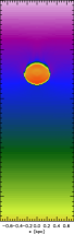
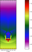
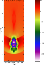
Figure 4: Model A1 ($n_{cloud}=0.01~{}\mbox{H atoms}~{}\mbox{cm}^{-3}$, $|\mbox{{\boldmath$B$}}|=0.0~{}\mu\mbox{G}$). The leftmost five plots show the $\mbox{log}_{10}$ of the hydrogen number density in units of atoms $\mbox{cm}^{-3}$ for a cut along the $y=0$ plane at $t=8,~{}16,~{}24,~{}32$, and $40~{}\mbox{Myr}$. The right-most plot shows $v_{z}$ in units of $\mbox{km}~{}\mbox{s}^{-1}$ for the material on the $y=0$ plane at $t=40~{}\mbox{Myr}$.

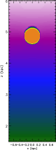
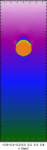
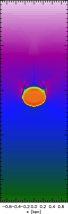
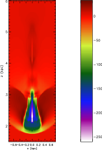
Figure 5: Same as Figure 4, but for Model A2 ($n_{cloud}=0.1~{}\mbox{H atoms}~{}\mbox{cm}^{-3}$, $|\mbox{{\boldmath$B$}}|=0.0~{}\mu\mbox{G}$).

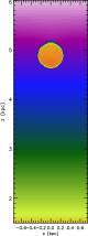
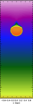
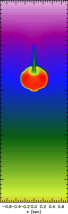
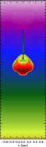
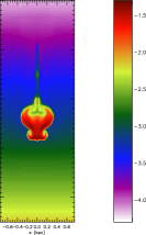
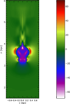
Figure 6: Same as Figure 4, but for Model B1 ($n_{cloud}=0.01~{}\mbox{H atoms}~{}\mbox{cm}^{-3}$, $B_{y}=1.3~{}\mu\mbox{G}$).

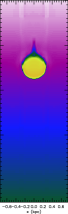
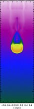
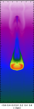
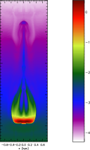
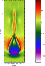
Figure 7: Same as Figure 4, but for Model B2 ($n_{cloud}=0.1~{}\mbox{H atoms}~{}\mbox{cm}^{-3}$, $B_{y}=1.3~{}\mu\mbox{G}$).

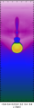
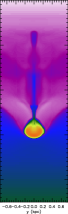
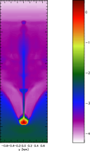
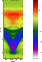
Figure 8: Same as Figure 7 for Model B2, but the cuts are along the $x=0$ plane.

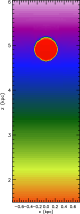
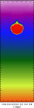
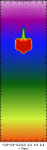
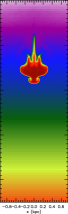
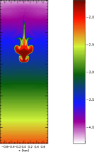
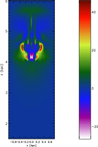
Figure 9: Same as Figure 4, but for Model B3 ($n_{cloud}=0.01~{}\mbox{H atoms}~{}\mbox{cm}^{-3}$, $B_{y}=4.2~{}\mu\mbox{G}$).

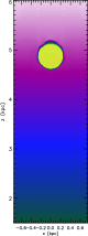
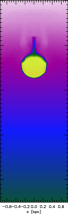
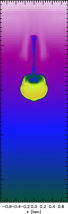
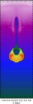
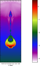
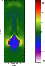
Figure 10: Same as Figure 4, but for Model B4 ($n_{cloud}=0.1~{}\mbox{H atoms}~{}\mbox{cm}^{-3}$, $B_{y}=4.2~{}\mu\mbox{G}$).

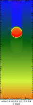
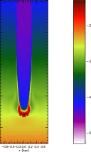
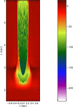
Figure 11: Same as Figure 4, but for Model C1 ($n_{cloud}=0.01~{}\mbox{H atoms}~{}\mbox{cm}^{-3}$, $B_{z}=1.3~{}\mu\mbox{G}$).

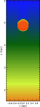
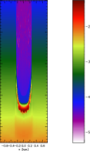
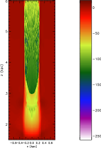
Figure 12: Same as Figure 4, but for Model C2 ($n_{cloud}=0.01~{}\mbox{H atoms}~{}\mbox{cm}^{-3}$, $B_{z}=4.2~{}\mu\mbox{G}$).

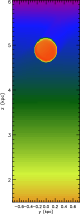
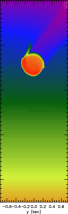
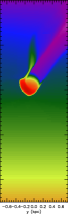
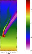
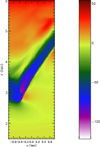
Figure 13: Same as Figure 4, but for Model D ($n_{cloud}=0.01~{}\mbox{H atoms}~{}\mbox{cm}^{-3}$, $B_{y}=B_{z}=0.94~{}\mu\mbox{G}$) and the cuts are on the $x=0$ plane.

In the upper cloud–ISM interface, a rarefaction wave propagates into the cloud and into the ISM, respectively. This is also similar to another case of the one-dimensional shock tube problem, in which a high-density region moves away from a neighboring low-density region of the same thermal plus magnetic pressure (our cloud initially has the same thermal plus magnetic pressure as the neighboring gas). The rarefaction waves result in rarefied density regions behind the clouds in our simulations. The left five panels of Figures 4-13, which display the hydrogen number densities for the clouds and ambient media at times of 8, 16, 24, 32, and 40 Myr, show that these low-density regions develop during the cloud’s descent. Note that the rarefied regions are most clearly shown in Models A1 and A2 which have no ambient magnetic field and in Models C1, C2, and D in which the magnetic field is oriented parallel to the fluid’s velocity vector, while they are less clear in Models B1-B4 in which the magnetic field is oriented perpendicular to the fluid’s velocity vector. This is because clouds deform differently when the magnetic field is oriented perpendicular to the cloud’s motion. The effect of the magnetic field on the cloud’s morphology will be discussed in more detail in Section 4.3.2.

Note that the cloud–ISM interfaces in our model simulations do not exactly match the one-dimensional shock tube problem. Our clouds have spherical shapes, both our interstellar density and thermal pressure have gradients, and both the cloud and the ISM are affected by the gravity. Therefore, the jump in the thermal and magnetic pressure across the lower cloud–ISM interface is not constant in our simulations, in contrast with the shock tube profiles shown in Figure 3. In our simulations, there are gradients in the thermal and magnetic pressures across the lower cloud-ISM interface and these gradients provide resistance to the cloud’s motion. The shock tube profiles imply that this resistance increases with the magnetic field strength when the magnetic field lines are perpendicular to the cloud’s motion.

4.3 Results of Model Simulations

4.3.1 Dynamics of the Cloud

The cloud’s dynamics are affected by two factors, the cloud’s initial density and the orientation and strength of the ambient magnetic field. Denser clouds fall faster than less dense clouds in the same interstellar environment. Resistance to the cloud’s motion increases with the strength of the magnetic field when the magnetic field is oriented perpendicular to the cloud’s motion. The magnetic field effects are more important when the cloud’s initial density is small.

Physically, the acceleration of the cloud is determined from the competition between the gravitational force of the Galaxy and the resisting force developed via the cloud-ISM interaction. The net acceleration of the cloud ($\vec{a}$) is

$$\vec{a}=\vec{g}-\frac{\hat{z}}{\rho_{cl}}(\frac{dp_{tot}}{dz}),$$ (1)

where $\rho_{cl}$ is the cloud’s density, $p_{tot}$ is the total pressure, $p_{tot}=p_{th}+p_{mag}$, $p_{th}$ is the thermal pressure, and $p_{mag}$ is the magnetic pressure. The values of $(a/g)$, calculated from $(\frac{dp_{tot}}{dz})$, $\rho_{cl}$, and $g(z)$ which are garnered from the simulations at $t=$8, 16, 24, and 32 Myr, are shown in Table 2. The distances that the clouds have fallen by $t=$16 and 24 Myr are also estimated for comparison.

The estimated values of ($a/g$) decrease over time because resistance due to the cloud-ISM interaction increases over time. Comparison between Models A1 and A2, Models B1 and B2, and Models B3 and B4, in which the cloud’s initial densities vary while the ambient magnetic field has the same orientation and strength, confirms that the heavier clouds fall faster. The negative correlation between the magnetic field strength and the resistance to motion is confirmed by comparing Model A1 in which there is no magnetic field with Models B1 and B3 which have small and large magnetic fields, respectively. These three models have small initial cloud densities. The comparison between Models A2, B2, and B4, in which the clouds have large initial densities, generally exhibits the same trend, but the fields are too weak to significantly decelerate the heavy cloud at early times.

4.3.2 Geometrical Consequences for the Cloud and the ISM

Our simulations show that the magnetic field affects not only the cloud’s dynamics but also the cloud’s morphology. In this subsection, we discuss four geometrical consequences for the cloud and the ISM; creation of tail structures, flattening of the cloud, asymmetric shape change, and the effect of a tilted magnetic field.

In each model, the cloud develops a tail due to the shear between the cloud and the ISM, but the shape and length of the tail is affected by the magnetic field orientation and strength. Especially in Models C1 and C2, where the magnetic field is oriented parallel to the cloud’s motion, a very thin tail develops along the sides of the columnar-shaped region behind the cloud. This region has a higher magnetic field strength than the surrounding gas and can be identified as a low-density region behind the cloud in the density profiles of Figures 11 and 12. Because its strong magnetic field protects the region behind the cloud from substantial inflows, the material sheared off of the cloud cannot invade this region and, instead, is confined along the sides of the high magnetic field wall.

The clouds deform as they fall. Due to both the ISM’s force on the cloud and the gradient in the Galaxy’s gravitational acceleration, the clouds flatten into disk- or cigar-shaped objects depending on the orientation of the interstellar magnetic field. For example, by 40 Myr the cloud in Model A2 deforms into a disk shape which has a radius of $\sim 0.23$ kpc and a depth of $\sim 0.1$ kpc. By the same time, the cloud in Model B2 has deformed into a cigar shape which has lengths of $\sim 0.65$ kpc along $x$-axis and $\sim 0.26$ kpc along $y$-axis and a height of $\sim 0.13$ kpc. We will discuss the observational effect of these flattened clouds in Section 5.1. In addition to flattening, instabilities result in downward protruding nodules.

In the cases where the magnetic field is oriented perpendicular to the cloud’s motion (Models B1-B4 and Model D which also has a magnetic field component that is perpendicular to $\hat{z}$), the cloud loses its symmetry about the $z$-axis. This is shown, for example, by comparing Figures 7 and 8. Both figures show the three-dimensional simulation results of Model B2, but Figure 7 displays the cut through the $y$-$z$ plane ($x=0$ plane), while Figure 8 shows the cut through the $x$-$z$ plane ($y=0$ plane). The magnetic field is oriented along the $y$-axis (i.e., $B_{y}\neq 0$) in this simulation, thus the magnetic field lines are coming into the plane in Figure 7, while they are parallel to the horizontal axis in Figure 8. The information in Figures 7 and 8 helps demonstrate the cloud’s three-dimensional morphology and how it evolves. As time elapses, the initially spherical cloud is squeezed along the direction of the initial magnetic field ($y$-axis), but is allowed to expand along the direction perpendicular to the initial magnetic field ($x$-axis). Note that this trend is the opposite of that experienced by bubbles in the ISM (Gaensler 1998; Raley et al. 2007), in which the elongation is parallel to the magnetic field direction. In our simulations, the cloud’s deformation grows with time so that by $t=40~{}\mbox{Myr}$, the cloud’s footprint looks like a bar which is elongated along the $x$-axis. The ambient magnetic field folds around the deformed cloud and makes a deep “V” shape in the $y$-$z$ plane. In contrast, in the cases where there is no magnetic field component parallel to the Galactic plane, the cloud retains cylindrical symmetry about the $z$-axis. Thus, the simulation results of Models A1, A2, C1, and C2 for cuts through the $y$-$z$ plane ($x=0$ plane) are identical to the results for cuts through the $x$-$z$ plane ($y=0$ plane) shown in Figures 4, 5, 11, and 12.

In Model D, the magnetic field lines are oriented at a $45\arcdeg$ angle with respect to the Galactic plane. The important consequence of this magnetic field configuration is that the cloud’s path is guided by the magnetic field lines. However, the cloud’s downward acceleration is still affected only by the magnetic field component that is perpendicular to $\hat{z}$ (i.e., $B_{y}$). The strength of this $B_{y}$ component in Model D is about $0.94~{}\mu\mbox{G}$ which is $1/\sqrt{2}$ times as strong as the magnetic strength in Model B1. As a result, the cloud’s vertical acceleration in Model D is between those of Model A1 and Model B1. The effect of the magnetic field component parallel to $\hat{z}$ ($B_{z}$) is to create a high magnetic pressure region behind the cloud, along whose sides tails develop. However, unlike in Models C1 and C2, the tail is asymmetric. The tail near the bottom of the cloud is suppressed, while the tail near the top of the cloud grows and spreads widely.

4.3.3 Vertical Velocities

In order to investigate which model clouds achieve fast enough speeds to be identified as HVCs, we examine their downward velocities. We examine the clouds late in their descents ($t=40~{}\mbox{Myr}$) because they move faster at this time than at any previous time. At later times, some of the clouds will cross the Galactic plane or slow dramatically. Figures 14 and 15 show the distribution of material across the velocity range $-150\leq v_{z}\leq-40$ $\mbox{km}~{}\mbox{s}^{-1}$. Table 3 presents the ratio of the gas mass to the initial cloud’s mass in five $v_{z}$ ranges for each model.

Among all of the simulated clouds, those in Models A2 and B2 (which have initial densities of $0.1~{}\mbox{H atoms}~{}\mbox{cm}^{-3}$) are most likely to be identified as HVCs after falling from rest for 40 Myr. In these simulations, the amount of material with $v_{z}\leq-90$ $\mbox{km}~{}\mbox{s}^{-1}$ is comparable to the cloud’s initial mass. The cloud in Model B4 (which has the same initial density as those in Models A2 and B2) would be observed as an IVC rather than as an HVC because most of the material has vertical velocities between $-90$ and $-40$ $\mbox{km}~{}\mbox{s}^{-1}$. In comparison, the low density analogs to the clouds in Models A2 and B2 (i.e., Models A1 and B1, respectively) would appear to the observers as IVCs and the low density analog to the Model B4 cloud (i.e., the Model B3 cloud) would appear as an even slower class of cloud.

The results for Models B1-B4, and D listed in Table 3 confirm that the ability of the ISM to retard the cloud’s motion increases with the strength of the component of the magnetic field that is perpendicular to the cloud’s velocity vector. While the Model B2 cloud moves at HVC velocities, its high magnetic field analog (the Model B4 cloud) moves at IVC velocities. Similarly, the Model B1 cloud mostly moves at IVC velocities while its high magnetic field analog (the Model B3 cloud) moves much slower. In Model D, whose $B_{y}$ is smaller than that of B1, the mass fraction in the range of IVC velocities is larger than that in Model B1. The cloud in Model D would also be identified as an IVC.

The results for Models C1 and C2 listed in Table 3 confirm that magnetic fields that run parallel to the cloud’s motion do not slow the clouds as effectively as fields that cross the cloud’s motion vector. However, the more detailed velocity distributions for these models shown in Figure 15 reveal that the effects of magnetic fields that are oriented parallel to the cloud’s motion increase with magnetic field strength. To wit, the velocity distribution for Model C2 is skewed to lower velocities, implying that the cloud in this model experienced more resistance than those in Models C1 and A1, which, respectively, have $1/\sqrt{10}$ and 0 times the magnetic field strength of Model C2. Note that a significant amount of material in Model C2 travels at $-60\leq v_{z}\leq-40$ $\mbox{km}~{}\mbox{s}^{-1}$. Most of this material is ambient ISM located ahead of the cloud. Models C1 and A1 also have accelerated ambient gas, though less of it.

The stronger magnetic field in Model C2 more tightly confines the lateral spread of both the cloud and the compressed ISM below the cloud. The pressure of the small confined region below the Model C2 cloud provides slightly larger resistance than the pressure of the larger region below the Model C1 cloud. In Model A1, the zone of high pressure is spread out even further than in Model C1 and provides even less resistance to the cloud’s descent. Thus, the cloud in Model C2 experiences more resistance than those in Models A1 and C1 (compare the $v_{z}$ profiles in Figures 4, 11, and 12). In addition, the shock wave propagates faster in the more pressurized, more confined region below the cloud in Model C2. But, in Models A1 and C1, the shock waves stall in the region where the pressure is weakened. The shock wave is important because the ambient material in the velocity range of $-60\leq v_{z}\leq-40$ $\mbox{km}~{}\mbox{s}^{-1}$ gained its velocity when the shock wave passed it.

In addition to downward-moving gas, we also find upward-moving gas by $40$ Myr (Table 3, sixth column). The upwardly moving material is ambient gas that was pushed aside by the falling clouds and now moves upward along the sides of the clouds. Gravity eventually stops this upwardly moving gas material and returns it to HSE. The behavior of the ambient gas through which a cloud falls, especially in Models A1 and A2 in which there is no ambient magnetic field, is similar to water through which a rock falls. At any instant, there is a portion of water that moves downward because it was pushed down by the rock; but the water is not permanently dragged down with the rock. Instead, it returns to its original hydrostatic balance after the rock passes through it. The fourth and sixth column in Table 3 show that roughly similar amounts of gas material move in the ranges of $-40\leq v_{z}\leq-10$ and $v_{z}\geq 10$ $\mbox{km}~{}\mbox{s}^{-1}$, resulting from the above behavior of the ambient gas in Models A1-B4. However, the upward motion of the ambient gas in Models C1 and C2 is significantly inhibited due to the magnetic field oriented along the $z$-direction. In these cases, the magnetic field acts like a cage that prevents the compressed ambient gas from moving laterally. Because it cannot easily flow around the cloud, the ambient material is dragged down with the cloud in Models C1 and C2. Although it is very unlikely that many infalling clouds are directed along the ambient magnetic field of the lower Galactic halo, this additional gas dragged with the cloud theoretically increases the mass return rate of the fountain process. It is interesting to compare the mass of the ambient gas that is dragged down in Models C1 and C2 with the results of Fraternali & Binney (2006, 2008). They modeled the extraplanar neutral gas for two nearby galaxies, NGC 891 and NGC 2403 and they found that the observed dynamics can be explained if the extraplanar gas is composed of $80\%$-$90\%$ of fountain gas that accretes $10\%$-$20\%$ extra gas material from the ambient medium during its descent. Note that their model assumes point particles for the fountain gas and includes the Galaxy’s gravity when calculating the trajectories of the particles. In their model, the estimated accretion rate was a model parameter and was determined by comparison with observations. Our simulations show that dragging of ambient gas can be significant depending on the configuration of the ambient magnetic field.

Table 3 also lists significant mass fractions of slow moving gas (i.e., $-10\leq v_{z}\leq 10~{}\mbox{km}~{}\mbox{s}^{-1}$). This is not astronomically significant. It is due to the disruption of the ambient medium and the imperfect numerical implementation of HSE. However, in Model B3, $80\%$ of the cloud mass is in this velocity range; the ISM motions merely mask the motion of this very slowly descending cloud.

In only one of our cases, that with the lowest cloud density and the highest magnetic field strength (Model B3), does the cloud reach terminal velocity. On the surface, this may seem to contradict the analytical calculation of Benjamin & Danly (1997) who assumed and validated the assumption that downward falling fountain gas reaches terminal velocity. However, their comparisons between theory and observations concentrated on IVCs, most of which were observed within 200 pc of the Galactic plane and were thought to have fallen from heights of approximately $z=1$ kpc. In our simulations, the clouds fall from a height of $z=5$ kpc where the gravitational acceleration is stronger and the interstellar density is weaker than at $z=1$ kpc (see Figure 1) and we do not track the clouds below a height of $z\approx 2$ kpc. Another difference between our work and that of Benjamin & Danly (1997) is that they assume that the drag coefficient remains constant throughout time, but we find that the drag changes as the magnetic field and gas are compressed beneath the cloud causing $d(p_{mag}+p_{th})/dz$ across the cloud-ISM interface to increase. In our simulations, the drag is too small to decelerate the clouds to the terminal velocity in all but Model B3.

5 Discussion

5.1 How Column and Volume Densities Relate to Observations

The calculated column densities of fast-moving gas ($v_{z}\leq-90~{}\mbox{km}~{}\mbox{s}^{-1}$) along the $z$-axis at $x=y=0$ in Models A2 and B2 are approximately $2.73\times 10^{20}$ and $5.0\times 10^{20}$ $\mbox{cm}^{-2}$, respectively. They are larger than the analytically calculated column density for the equivalent line of sight through a ballistically falling cloud having an initial density of 0.1 H atoms $\mbox{cm}^{-3}$ and a radius of 0.25 kpc ($1.5\times 10^{20}~{}\mbox{cm}^{-2}$, see Section 4.1) because the simulated clouds have accelerated ambient material. The Model B2 cloud has a larger column density than the Model A2 cloud because more material accumulates along the central sight line when the magnetic field lines are perpendicular to the cloud’s motion (Section 4.3.2). Note that the HVC column densities in both Models A2 and B2 exceed the detection threshold for most HVC observations (a few times $10^{18}~{}\mbox{cm}^{-2}$).

An interesting comment needs to be made about calculations of the volume density that draw upon observational data. In such cases, the volume density, $n$, is usually estimated from the column density, $N$, by using the equation $n=N/d$, where $d$ is the depth of the cloud. Since $d$ is not observable, it is often assumed to be equal to the cloud’s width. However, as in our simulations, if a cloud is compressed vertically during its descent, or is deformed either due to compression or due to the magnetic field, then the above assumption is not applicable. In the cases where the cloud is more compressed vertically than horizontally, its depth is smaller than its width and so the volume density calculated with the above technique underestimates the real volume density of the cloud. For example, this occurs in Models A2 and B2. We measured the cloud’s dimensions for Models A2 and B2 at 40 Myr (Section 4.3.2). If the width of the cloud is used as $d$ for the volume density estimation, then the estimated volume density is approximately $0.19~{}\mbox{H atoms}~{}\mbox{cm}^{-3}$ and $0.25~{}\mbox{H atoms}~{}\mbox{cm}^{-3}$ for the cloud of Models A2 and B2, respectively. However, the mean volume density measured from the simulation is approximately $0.56~{}\mbox{H atoms}~{}\mbox{cm}^{-3}$ and $2.13~{}\mbox{H atoms}~{}\mbox{cm}^{-3}$ for Models A2 and B2, respectively.

5.2 Magnetic Field Geometries in the Galactic Fountain

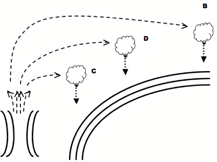
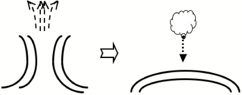
Figure 16: Possible magnetic geometries in the context of a Galactic fountain. The solid lines are magnetic field lines and the dashed and dotted lines show possible paths of the fountain gas. See the text for a detailed explanation.

Figure 16 shows two possible scenarios describing the geometry of the magnetic field in the context of a Galactic fountain model. In both figures, magnetic field lines surrounding interstellar bubbles are indicated by the solid lines and possible paths of the fountain gas are represented by the dashed lines. In the left figure, hot gas escapes from a hot bubble, moves upward, and possibly to the side, cools down, and condenses into clouds at various possible locations with respect to a neighboring bubble. The magnetic field lines of the neighboring bubble are assumed to be aligned along its periphery. As a result, clouds B-D (corresponding to the models in Table 1 whose names begin with the letters B-D) encounter different magnetic field geometries during their descents. The magnetic field geometries are parallel, perpendicular and tilted at $45\arcdeg$ with respect to the Galactic plane in Models B-D, respectively.

The right figure shows a second possible scenario. In it, hot gas escapes from a hot bubble. While this gas cools down and condenses, the bubble’s magnetic field lines, that had been breached to let the hot gas out, reform. In this case, the cloud falls back down near the region where the hot gas escaped. If the condensed gas cloud falls onto the top of the bubble, then it encounters a magnetic field that is parallel to the Galactic plane, like in Model B. If the escape region is on the sides of the bubble or somewhere between the top and the side, then the cloud will encounter a magnetic field that is perpendicular to or at a $45\arcdeg$ angle to the plane, as in Model C or D, respectively.

5.3 Recombination of Ionized Gas

The magnetic field only acts directly upon the ionized gas. It does not act directly on neutral particles, although it does act on ionized particles that are mixed in with neutral particles and the ionized particles will influence the neutral particles. Technically, those of our simulations that include magnetic fields assume that both the cloud and the ambient ISM are ionized. If the ionized cloud recombines later, it could be observed as a neutral HVC. Even if the ionized cloud does not fully recombine, the MHD simulations are still relevant because partially and fully ionized HVCs have been observed (Sembach et al. 2003; Fox et al. 2006).

5.4 Hot Ambient Medium

Within 5 kpc of the Milky Way’s midplane, the ISM contains hot, warm, and cool gas. Recent observations revealed that even cold gas (H I) contributes a significant portion of the halo ISM in the Milky Way (Kalberla & Dedes 2008) and an external galaxy, NGC 891 (Oosterloo et al. 2007). However, there is evidence that hot ($>10^{6}$ K) gas plays a more dominant role in some galaxies. The halos of starburst galaxies, for example, contain significant quantities of hot gas (e.g., Strickland et al. (2004)). In addition, Fukugita & Peebles (2006) suggested that the very extended halos of normal spiral galaxies are hot. If a cloud was to fall through a hotter more rarefied gas than we assumed in our simulations, then it would experience less resistance due to the thermal pressure gradient. This effect would be most relevant if the magnetic field was absent or oriented parallel to the cloud’s motion and would allow the cloud to fall slightly faster than the clouds in Models A1, A2, C1, and C2. If, in contrast, a non-negligible magnetic field oriented perpendicular to the cloud’s motion was to permeate the halo, then the thermal pressure gradient would be unimportant. The buildup of magnetic pressure beneath the cloud would dominate the cloud’s dynamics. This magnetic pressure would slow the cloud, regardless of the reduced thermal pressure.

6 Conclusion

Our simulations show that some clouds that form in the Galactic fountain process can be observed as HVCs during their descent toward the Galactic plane. According to our simulations, a cloud is more likely to accelerate to HVC-class velocities if its initial density is large enough to overcome the interaction with the ambient ISM. The interaction with the ambient ISM depends upon the configuration of the magnetic field in the Galactic halo. Magnetic fields that are parallel to the Galactic plane decelerate the falling cloud most effectively, while magnetic fields that are perpendicular to the plane and thus parallel to the motion of the cloud merely confine the material and guide its trajectory, but do not significantly slow the cloud. The strength of the magnetic field is important to the motion of the cloud only when the magnetic field is perpendicular to the cloud’s motion. In this case, the cloud’s downward movement compresses and thus strengthens the magnetic field. Unless the density of the cloud is sufficiently large, the resulting magnetic pressure controls the cloud’s dynamics.

We find that an initial cloud density of $0.1~{}\mbox{H atoms}~{}\mbox{cm}^{-3}$ is large enough for the cloud to overcome the interaction with the ambient ISM if the ambient magnetic field strength is $\leq 1.3~{}\mu$G, regardless of the magnetic field’s orientation. Since an ambient magnetic field with this strength or less is very likely to exist at the cloud’s maximum height above the Galactic plane, clouds with this density or greater that fall from the height of $z=5$ kpc should accelerate to $|v|>90$ $\mbox{km}~{}\mbox{s}^{-1}$ and therefore be easily identified as HVCs after they fall for about 40 Myr. However, if the ambient magnetic field is perpendicular to the motion of the cloud and has a relatively large strength ($\geq 4.2~{}\mu$G), then the cloud’s interaction with the ISM is stronger and significantly hinders the cloud’s motion. A cloud falling in such an environment for 40 Myr is more likely to be identified as an IVC than as an HVC. If the initial cloud density is 1/10 of the above density, then the cloud reaches HVC velocities during its fall only if the magnetic field is absent or parallel to the cloud’s motion.

Figure 1: The physical state of the Galactic halo gas assumed in the simulations is shown. Top panels from left to right: hydrogen number density and gravitational acceleration as a function of height for regions at the Sun’s galactocentric radius, from Ferriere (1998). Molecular hydrogen is excluded from the density profile. We assume that the helium abundance in the halo gas is 10% of the hydrogen abundance. Bottom left panel: the total weight per unit area ($\mbox{erg}~{}\mbox{cm}^{-3}$) and two magnetic pressure values used in some simulations. The total weight per unit area is marked by the solid line, a magnetic pressure of $7.0\times 10^{-14}~{}\mbox{erg}~{}\mbox{cm}^{-3}$ (corresponding to a magnetic field strength of $1.3~{}\mu\mbox{G}$) is marked by the dotted line, and a magnetic pressure of $7.0\times 10^{-13}~{}\mbox{erg}~{}\mbox{cm}^{-3}$ (corresponding to a magnetic field strength of $4.2~{}\mu\mbox{G}$) is marked by the dashed line. Bottom right panel: assumed ambient temperature as a function of height.

Figure 2: Analytically calculated height and velocity of a cloud of the same size as the clouds used in our simulations as it falls in a vacuum under the gravitational acceleration shown in Figure 1. The heights (marked by thin curves that decrease from left to right) and downward speeds (marked by thick curves that increase from left to right) are shown as a function of time after the cloud begins to fall from rest. The dotted, dashed, and dot-dashed lines correspond to the top, center, and bottom of the cloud, respectively. At the beginning of the time period, the top, center, and bottom of the cloud are located at 5.25, 5.0, and 4.75 kpc, respectively. The solid vertical line marks 40 Myr.

Figure 3: One-dimensional shock tube profiles corresponding to the lower interface between the cloud and the ambient ISM in our simulations. The initial contact discontinuity is located at $x=0$ kpc and the plots are made at $t=18$ Myr. Different lines correspond to shock tube models that have the same densities and magnetic field strengths as we use in our HVC simulations; thick solid line (Model A2), thick dashed line (Model B2), thick dotted line (Model B4), thin solid line (Model A1), thin dashed line (Model B1), and thin dotted line (Model B3). In the hydrogen number density profile (top left panel), the reverse shock, contact discontinuity, and forward shock appear as each sudden change from left, respectively. Note that the contact discontinuity is the cloud-ISM interface and its locations in different models do not vary much. The velocity, thermal pressure and magnetic pressure profiles are shown in the top right, bottom left, and bottom right panels, respectively. Note that these physical variables do not change across the contact discontinuity.

Figure 14: Mass of material moving vertically with a velocity of $v_{z}$ at 40 Myr for models with a high initial cloud density: A2 (solid line), B2 (dotted line) and B4 (dashed line). The normalized mass ratios on the $y$-axis are calculated from the mass of gas material within a velocity range by dividing by the initial mass of the cloud and by the width of the velocity bin ($\Delta v_{z}=2.0~{}\mbox{km}~{}\mbox{s}^{-1}$ in this plot). The total mass of material within the $-40\leq v_{z}\leq-150~{}\mbox{km}~{}\mbox{s}^{-1}$ velocity range exceeds the cloud’s mass in cases where the ambient gas has been accelerated.

Figure 15: Mass of material moving with a velocity of $v_{z}$ at 40 Myr for models with a low initial cloud density: A1 (thick dotted line), B1 (thin solid line), C1 (dashed line), C2 (thick solid line), and D (thin dotted line). Note that there is no material moving within this velocity range in Model B3. The normalized mass ratios are calculated in the same way as those in Figure 14.

Table 1: Models

Models	Cloud Density	Magnetic Pressure	Magnetic Orientation
	(H atoms $\mbox{cm}^{-3}$)	($10^{-14}$ erg $\mbox{cm}^{-3}$)
A1	0.01	0.0	$\cdots$
A2	0.1	0.0	$\cdots$
B1	0.01	7.0	Perpendicular
B2	0.1	7.0	Perpendicular
B3	0.01	70.0	Perpendicular
B4	0.1	70.0	Perpendicular
C1	0.01	7.0	Parallel
C2	0.01	70.0	Parallel
D	0.01	7.0	$45\arcdeg$

Table 2: $a/g$ and Distance Fallen

	Cloud	Magnetic	$a/g$				Distance Fallen (kpc)
Models	Density	Field	———————————————–				——————————
	(H atoms $\mbox{cm}^{-3}$)	($B_{y}$ in $\mu\mbox{G}$)	8 Myr	16 Myr	24 Myr	32Myr	16 Myr	24 Myr
A1	0.01	0.0	0.91	0.80	0.70	0.56	0.71	1.24
A2	0.1	0.0	0.97	0.92	0.83	0.94	0.74	1.34
B1	0.01	1.3	0.88	0.48	0.38	0.22	0.61	0.97
B2	0.1	1.3	0.96	0.95	0.87	0.73	0.71	1.28
B3	0.01	4.2	0.74	0.73	0.55	0.06	0.49	0.66
B4	0.1	4.2	0.96	0.77	0.69	0.20	0.67	1.19

Table 3: Fraction of Cloud Mass Traveling within a Given Velocity Range at $40$ Myr

Models	$v_{z}\leq-90$	$-90\leq v_{z}\leq-40$	$-40\leq v_{z}\leq-10$	$-10\leq v_{z}\leq 10$	$v_{z}\geq 10$
	( $\mbox{km}~{}\mbox{s}^{-1}$ )	( $\mbox{km}~{}\mbox{s}^{-1}$ )	( $\mbox{km}~{}\mbox{s}^{-1}$ )	( $\mbox{km}~{}\mbox{s}^{-1}$ )	( $\mbox{km}~{}\mbox{s}^{-1}$ )
A1	0.25	0.91	2.81	16.39	1.68
A2	1.0	0.09	0.3	1.41	0.25
B1	0.0	0.62	0.55	20.08	0.54
B2	0.95	0.1	0.41	1.25	0.28
B3	0.0	0.0	0.21	21.64	0.24
B4	0.03	0.94	0.11	1.68	0.26
C1	0.19	1.02	0.93	19.48	0.13
C2	0.02	1.59	0.99	19.28	0.0
D	0.0	1.01	0.44	16.72	0.35

Note. — The fractions sum to $>1.0$ because ambient material has been counted along with the cloud material.

References

- Agertz et al. (2007) Agertz, O., et al. 2007, MNRAS, 380, 963
- Belokurov et al. (2007) Belokurov, V., et al. 2007, ApJ, 654, 897
- Benjamin & Danly (1997) Benjamin, R. A., & Danly, L. 1997, ApJ, 481, 764
- Blitz et al. (1999) Blitz, L., Spergel, D. N., Teuben, P. J., Hartmann, D., & Burton, W. B. 1999, ApJ, 514, 818
- Collins et al. (2007) Collins, J. A., Shull, J. M., & Giroux, M. L. 2007, ApJ, 657, 271
- Cowie & McKee (1977) Cowie, L. L., & McKee, C. F. 1977, ApJ, 211, 135
- Danly et al. (1993) Danly, L., Albert, C. E., & Kuntz, K. D. 1993, ApJ, 416, L29
- Davis et al. (1996) Davis, D. S., Mulchaey, J. S., Mushotzky, R. F., & Burstein, D. 1996, ApJ, 460, 601
- de Avillez (2000) de Avillez, M. A. 2000, Ap&SS, 272, 23
- de Avillez & Breitschwerdt (2007) de Avillez, M. A., & Breitschwerdt, D. 2007, ApJ, 665, L35
- Ferriere (1998) Ferriere, K. 1998, ApJ, 497, 759
- Fox et al. (2006) Fox, A. J., Savage, B. D., & Wakker, B. P. 2006, ApJS, 165, 229
- Fraternali & Binney (2006) Fraternali, F., & Binney, J. J. 2006, MNRAS, 366, 449
- Fraternali & Binney (2008) —. 2008, MNRAS, 386, 935
- Fryxell et al. (2000) Fryxell, B., et al. 2000, ApJS, 131, 273
- Fukugita & Peebles (2006) Fukugita, M., & Peebles, P. J. E. 2006, ApJ, 639, 590
- Gaensler (1998) Gaensler, B. M. 1998, ApJ, 493, 781
- Gibson et al. (2000) Gibson, B. K., Giroux, M. L., Penton, S. V., Putman, M. E., Stocke, J. T., & Shull, J. M. 2000, AJ, 120, 1830
- Jones et al. (1996) Jones, T. W., Ryu, D., & Tregillis, I. L. 1996, ApJ, 473, 365
- Kalberla & Dedes (2008) Kalberla, P. M. W., & Dedes, L. 2008, A&A, 487, 951
- Keenan et al. (1995) Keenan, F. P., Shaw, C. R., Bates, B., Dufton, P. L., & Kemp, S. N. 1995, MNRAS, 272, 599
- Kudoh & Basu (2004) Kudoh, T., & Basu, S. 2004, A&A, 423, 183
- Kuntz & Danly (1996) Kuntz, K. D., & Danly, L. 1996, ApJ, 457, 703
- LeVeque (2002) LeVeque, R. J. 2002, Finite Volume Methods for Hyperbolic Problems (Cambridge University Press)
- Lu et al. (1998) Lu, L., Sargent, W. L. W., Savage, B. D., Wakker, B. P., Sembach, K. R., & Oosterloo, T. A. 1998, AJ, 115, 162
- Mac Low et al. (1994) Mac Low, M.-M., McKee, C. F., Klein, R. I., Stone, J. M., & Norman, M. L. 1994, ApJ, 433, 757
- MacNeice et al. (2000) MacNeice, P., Olson, K. M., Mobarry, C., deFainchtein, R., & Packer, C. 2000, Comput. Phys. Commun., 126, 330
- McKee & Begelman (1990) McKee, C. F., & Begelman, M. C. 1990, ApJ, 358, 392
- Muller et al. (1963) Muller, C. A., Oort, J. H., & Raimond, E. 1963, C.R. Acad. Sci. Paris, 257, 1661
- Oort (1966) Oort, J. H. 1966, Bull. Astron. Inst. Netherlands, 18, 421
- Oosterloo et al. (2007) Oosterloo, T., Fraternali, F., & Sancisi, R. 2007, AJ, 134, 1019
- Putman et al. (2004) Putman, M. E., Thom, C., Gibson, B. K., & Staveley-Smith, L. 2004, ApJ, 603, L77
- Raley et al. (2007) Raley, E. A., Shelton, R. L., & Plewa, T. 2007, ApJ, 661, 222
- Santillán et al. (1999) Santillán, A., Franco, J., Martos, M., & Kim, J. 1999, ApJ, 515, 657
- Schwarz et al. (1995) Schwarz, U. J., Wakker, B. P., & van Woerden, H. 1995, A&A, 302, 364
- Sembach et al. (2003) Sembach, K. R., et al. 2003, ApJS, 146, 165
- Shapiro & Field (1976) Shapiro, P. R., & Field, G. B. 1976, ApJ, 205, 762
- Slavin et al. (1993) Slavin, J. D., Shull, J. M., & Begelman, M. C. 1993, ApJ, 407, 83
- Strickland et al. (2004) Strickland, D. K., Heckman, T. M., Colbert, E. J. M., Hoopes, C. G., & Weaver, K. A. 2004, ApJS, 151, 193
- Tenorio-Tagle et al. (1986) Tenorio-Tagle, G., Bodenheimer, P., Rozyczka, M., & Franco, J. 1986, A&A, 170, 107
- Tenorio-Tagle et al. (1987) Tenorio-Tagle, G., Franco, J., Bodenheimer, P., & Rozyczka, M. 1987, A&A, 179, 219
- Thom et al. (2008) Thom, C., Peek, J. E. G., Putman, M. E., Heiles, C., Peek, K. M. G., & Wilhelm, R. 2008, ApJ, 684, 364
- Tufte et al. (1998) Tufte, S. L., Reynolds, R. J., & Haffner, L. M. 1998, ApJ, 504, 773
- Vieser & Hensler (2007a) Vieser, W., & Hensler, G. 2007a, A&A, 475, 251
- Vieser & Hensler (2007b) —. 2007b, A&A, 472, 141
- Wakker (2001) Wakker, B. P. 2001, ApJS, 136, 463
- Wakker et al. (2007) Wakker, B. P., et al. 2007, ApJ, 670, L113