The velocity function in the local environment from $\Lambda$CDM and $\Lambda$WDM constrained simulations

Abstract

Using constrained simulations of the local Universe for generic cold dark matter and for 1$\>{\rm keV}$ warm dark matter, we investigate the difference in the abundance of dark matter halos in the local environment. We find that the mass function within $20{\>h^{-1}\rm Mpc}$ of the Local Group is $\sim 2$ times larger than the universal mass function in the $10^{9}-10^{13}{\>h^{-1}\rm M}_{\odot}$ mass range. Imposing the field of view of the on-going HI blind survey ALFALFA in our simulations, we predict that the velocity function in the Virgo-direction region exceeds the universal velocity function by a factor of 3. Furthermore, employing a scheme to translate the halo velocity function into a galaxy velocity function, we compare the simulation results with a sample of galaxies from the early catalog release of ALFALFA. We find that our simulations are able to reproduce the velocity function in the $80-300\>{\rm km\,s^{-1}}$ velocity range, having a value $\sim 10$ times larger than the universal velocity function in the Virgo-direction region. In the low velocity regime, $35-80\>{\rm km\,s^{-1}}$, the warm dark matter simulation reproduces the observed flattening of the velocity function. On the contrary, the simulation with cold dark matter predicts a steep rise in the velocity function towards lower velocities; for $V_{max}=35\>{\rm km\,s^{-1}}$, it forecasts $\sim 10$ times more sources than the ones observed. If confirmed by the complete ALFALFA survey, our results indicate a potential problem for the cold dark matter paradigm or for the conventional assumptions about energetic feedback in dwarf galaxies.

1. Introduction

Despite the success of the $\Lambda$CDM paradigm in describing the large scale structure of the Universe, as has been attested by improved measurements of the CMB and the large scale clustering of galaxies (Seljak et al., 2006b; Komatsu et al., 2008), some potential problems remain for the model at smaller scales. One of these challenges is related to the prediction of the abundance of low mass galaxies. Numerical simulations within the $\Lambda$CDM model predict many more dark matter subhalos inside galactic-sized host halos than the actual number of observed satellite galaxies around the Milky Way (Klypin et al., 1999; Moore et al., 1999; Diemand et al., 2007; Springel et al., 2008). This discrepancy has been known as the “missing satellite problem”. Although some astrophysical processes can be responsible for the suppression of galaxy formation in small mass halos and lead to the solution of the problem (Somerville, 2002; Benson et al., 2002b, a; Gnedin & Kravtsov, 2006; Koposov et al., 2009), it is also possible to alleviate the discrepancy by adopting alternative models with a different type of dark matter.

Warm dark matter (WDM) models, for instance, predict significantly less substructure within halos (Colín et al., 2000; Bode et al., 2001). The free streaming length for dark matter particles depends on their intrinsic properties and establishes a cut-off scale for halo masses below which primordial density perturbations are wiped out. In the case of neutralinos, one of the favorite candidates for CDM models, with $m_{\chi}\sim 100$GeV, the scale is roughly $10^{-6}{\>{\rm M}_{\odot}}$ (Diemand et al., 2005). For WDM candidates, such as gravitinos with $m_{\tilde{G}}\sim 1$KeV (see Steffen 2006 for a recent review on gravitino cosmology), this scale is roughly $10^{10}{\>{\rm M}_{\odot}}$ (see section 2). Therefore, using the same cosmological parameters but different cut-off scales results in different predictions for the halo mass function (MF). At the low mass end the $\Lambda$WDM mass function is expected to be significantly lower than the $\Lambda$CDM mass function. Above the cut-off scale the differences vanish (e.g. Bode et al., 2001; Barkana et al., 2001).

Since for high density environments both models provide, conceptually different, solutions for the missing satellite problem it is also important to test their predictions for isolated systems in low density environments which are not affected by processes such as ram-pressure or tidal striping. A comparison between $\Lambda$WDM and $\Lambda$CDM is then free from these astrophysical phenomena and conclusions drawn from it are more closely related to the nature of dark matter itself. Such an approach has been employed for example by Blanton et al. (2008).

Even though low mass galaxies are difficult to detect, surveys such as the ongoing Arecibo Legacy Fast ALFA (ALFALFA) survey (Giovanelli et al., 2005a) are promising to make such comparison. ALFALFA is exploring the local HI Universe with a sky coverage of $7000$ deg² and it is designed to detect objects with masses as low as $3\times 10^{7}{\>{\rm M}_{\odot}}$ at a Virgo-cluster distance ($11.7{\>h^{-1}\rm Mpc}$) (Giovanelli et al., 2007). The survey is divided into two regions on the sky. One within the solid angle $07^{h}30^{m}<$R.A.(J2000.0)$<16^{h}30^{m}$ and $0\arcdeg<$DEC(J2000.0)$<+36\arcdeg$, which includes the Virgo cluster, and another region within the same declination range and $22^{h}<$R.A.(J2000.0)$<03^{h}$. In the reminder of this work, we will loosely refer to these two regions, additionally constrained to distances less than $20{\>h^{-1}\rm Mpc}$, as the “Virgo-direction region (VdR)” and “anti-Virgo-direction region (aVdR)” respectively. We note that the catalogs released by ALFALFA so far in these two regions effectively correspond to a high and a low density environment. The HI sources detected by ALFALFA are typically associated with star forming disk galaxies, spirals in rich clusters are less likely to be detected since these galaxies might be HI deficient (Solanes et al., 2001).

In order to make predictions on the abundance of low mass galaxies based on the $\Lambda$CDM and $\Lambda$WDM models for our local environment, it is advantageous to use constrained simulations (CSs) of the local universe (e.g. Bistolas & Hoffman, 1998; Mathis et al., 2002; Klypin et al., 2003). These simulations are constructed to reproduce the gross features of the nearby Universe, such as the Local Supercluster and the Virgo cluster. This can be achieved by setting the initial conditions of the simulations as constrained realizations of Gaussian fields, where actual observational data are used to impose the constraints. By using such simulations, biases which are present because of the particular structure of the local environment, are minimized and a better comparison between simulations and observations can be achieved.

Although the abundance of dark matter halos is usually quantified by the mass function, which describes the number density of halos as a function of mass, usually presented either in a differential or integral form (e.g. Reed et al., 2007; Lukić et al., 2007), an alternative approach is to use the velocity function, similarly defined as the number density of halos as a function of maximum circular velocity (e.g. Gonzalez et al., 2000). The advantage of the velocity function (VF) is that it can be compared more directly with observational results since it avoids the more complicated problem of relating dark matter halo masses to galaxy luminosities. Instead, the velocity function of galaxies can be theoretically estimated using the velocity function of halos by incorporating a model of baryonic infall; the only processes that affect the velocity function are those that modify the gravitational potential of galactic systems. In the present work we show analysis of both, the mass and velocity functions, but concentrate on the latter for comparisons with the ALFALFA survey.

The objective of our paper is to run a $\Lambda$CDM and a $\Lambda$WDM simulation of the local environment where the same set of constraints have been imposed and to compare the abundance and distribution of dark matter halos for the two cosmologies. In addition, the results are used to predict the abundance of HI sources that will be detected by the on-going HI blind survey ALFALFA.

The paper is organized as follows. In section 2 we describe the setting of the simulations. The definition of the coordinate system that we use to impose the field of view of ALFALFA in the CSs is described in section 3. In section 4 we present results on the abundance of dark matter halos. In section 5 we analyze in particular the abundance for the restricted Virgo-direction and anti-Virgo-direction regions cataloged by the ALFALFA survey to date and present predictions on the velocity function of HI sources. The summary and conclusions of our work are given in section 6.

2. Constrained simulations of the local environment

We chose the cosmological parameters for our simulations to be consistent with the WMAP 3-year results (Spergel et al., 2007): $\Omega_{m}=0.24$, $\Omega_{\Lambda}=0.76$, $H_{0}=100h\rm\,km\,s^{-1}Mpc^{-1}$ with $h=0.73$, $n=0.95$ and $\sigma_{8}=0.75$. For both cosmologies the theoretical (unconstrained) linear power spectrum at $z=0$ is shown in Fig. 1 (blue for CDM and red for WDM). The CDM power spectrum was computed from a Boltzmann code by W. Hu and was kindly provided to us.

2.1. $\Lambda$WDM simulation settings

The WDM power spectrum was computed by rescaling the CDM power spectrum using a fitting function that approximates the transfer function for a thermal WDM particle with $m_{WDM}=1\>{\rm keV}$. The filtering scale (or free-streaming length) for this WDM particle mass is $350{\>h^{-1}\rm kpc}$, or about $\sim 1.1\times 10^{10}{\>h^{-1}\rm M}_{\odot}$ for the filtering mass (following the definitions given by Bode et al. 2001). We used the fitting function from Viel et al. (2005) (see their eqs. 5-7) which is very similar to the one given by Bode et al. (2001), however, according to the authors, it is a better fitting formula for Boltzmann codes.

As stated by recent Lyman-$\alpha$ forest, CMB and galaxy clustering data (Viel et al., 2006; Seljak et al., 2006a), see also Miranda & Macciò (2007), the lower limit for the mass of thermal WDM candidates, for the case where WDM is the dominant form of dark matter, has been reported to be $m_{WDM}\sim 2\>{\rm keV}$ at the $2\sigma$ level. However, these estimates for thermal relics may be contaminated by systematic errors (see for example Boyarsky et al. (2008a) for a discussion on the complications associated to the Lyman-$\alpha$ forest method). For instance, the constraint given in Viel et al. (2006) would reduce to $m_{WDM}\geq 0.9\>{\rm keV}$ if the highest redshift bins of the Lyman-$\alpha$ forest data are rejected from the analysis and only the more reliable data based on $z<3.2$ is taken into account. In a recent paper, Boyarsky et al. (2008b) revisit the lower bounds on the mass of WDM particles and find $m_{WDM}\geq 1.7\>{\rm keV}$ ($2\sigma$ level). However, after discussing with detail the systematic uncertainties in their method they conclude that the mass bounds are reliable within $\sim 30\%$ of uncertainty. All these analysis put our choice of $m_{WDM}=1\>{\rm keV}$ close to the most recent lower bound, but it is a choice that is still not ruled out.

The velocity dispersion of the WDM particles needs, in principle, to be introduced in the initial conditions for the simulations since after all, it is what causes the smearing of small scale primordial perturbations. This is usually done by introducing a random velocity field according to a Fermi-Dirac distribution function (Bode et al., 2001; Colín et al., 2008). However, if this velocity dispersion field is introduced at random, a certain degree of white noise is generated (shot noise) due to the finite number of simulation particles which produces spurious small scale power in the WDM spectrum (see Fig.1 of Colín et al. 2008). The amplitude of the rms velocity of the random component to be added depends on the nature of the WDM particle and on the redshift of the initial conditions. For thermal relics, it is larger for higher redshifts and smaller particle masses. For $z=50$ the rms velocity is $\sim 2.2\>{\rm km\,s^{-1}}$ for $m_{WDM}=1\>{\rm keV}$ (following the formula given by Bode et al. 2001), far lower than the velocities induced by gravitational collapse of structures having scales larger than the minimum scale we can resolve within our simulations. Therefore we do not incorporate any random velocity field into our initial conditions.

To back our approach we computed the comoving Jeans length associated with a velocity dispersion of $2.2\>{\rm km\,s^{-1}}$. We found that the time to build up pressure support against gravitational collapse is similar to the collapse time for comoving scales of $\sim 33{\>h^{-1}\rm kpc}$, corresponding to a Jeans mass of $\sim 10^{6}{\>h^{-1}\rm M}_{\odot}$. Differences in the structure formation are only expected for masses of the order and below the Jeans mass, which is lower than the particle mass in our simulations (see below). Thus, the effect of thermal velocities is too small to have a notable effect on the abundance of low mass halos in our simulations. Still, they could have an impact in the inner part of halos (Colín et al., 2008). However, since the shot noise produced by their introduction has a large spurious effect, we decided not to include them in our simulations. For the purposes of this work, this has no consequences in our analysis.

2.2. Constrained simulations

The initial conditions for the constrained simulations were set up using the (Hoffman & Ribak, 1991) algorithm of constrained realizations of Gaussian random fields. Two types of data sets are used as input for the algorithm. The first data set is made of radial velocities of galaxies drawn from the catalogs: MARK III (Willick et al., 1997), surface brightness fluctuations (Tonry et al., 2001) and the Catalog of Nearby Galaxies (Karachentsev et al., 2004). Present epoch peculiar velocities are less affected by non-linear effects and are therefore imposed as linear constraints on the primordial perturbation field (Zaroubi et al., 1999). This approach follows the CSs performed by Kravtsov et al. (2002) and Klypin et al. (2003). The other data set is obtained from the catalog of nearby X-ray selected clusters of galaxies (Reiprich & Böhringer, 2002). Assuming the spherical top-hat model and using the virial parameters of a cluster the linear over-density of the cluster is derived. The estimated linear overdensity is imposed on the virial mass scale of the cluster as a constraint. The density and velocity fields on scales larger than 5${\>h^{-1}\rm Mpc}$ are strongly constrained by the imposed data.

Using the above initial conditions, we carried out the simulations using the code GADGET-2 (Springel, 2005). Both simulations follow the evolution of $1024^{3}$ dark matter particles from $z=50$ to $z=0$ in a box of size $L=64{\>h^{-1}\rm Mpc}$. The associated Nyquist frequency and fundamental mode are represented with vertical lines in Fig. 1. The dark matter particle mass is $m_{DM}=1.63\times 10^{7}{\>h^{-1}\rm M}_{\odot}$. The simulations were started with a fixed comoving softening length (Plummer-equivalent) of $\epsilon=1.6{\>h^{-1}\rm kpc}$. Once the corresponding physical comoving softening reached $\epsilon=0.8{\>h^{-1}\rm kpc}$, it was kept constant at this value.

Fig. 2 displays the projected dark matter distribution of the CSs at $z=0$ for the $\Lambda$CDM and the $\Lambda$WDM models respectively. The highest and lowest concentrations are colored red and black respectively. Both panels show the matter distribution within a slice that is $8{\>h^{-1}\rm Mpc}$ thick projected onto the X-Y plane and centered on $Z=24{\>h^{-1}\rm Mpc}$. The figure captures the Local Supercluster (LSC) which is the filamentary structure crossing the image plane horizontally. It is the most prominent feature. The locations of the virtual Local Group (LG) and the Virgo cluster are marked as well. A description of the identification of these objects will follow below. A visual inspection of the two figures already reveals a deficit of small scale structure in the $\Lambda$WDM simulation, as expected.

Halos in the simulations were identified using AHF, AMIGA’s halo finder (Knollmann & Knebe, 2009). AHF identifies halos as local density maxima in an adaptively smoothed density field using a hierarchy of grids and a refinement criterion. The latter was chosen so that a grid cell is subdivided until each subsection contains less than 5 particles. In this way, the size of the smallest cells is comparable to the force resolution of our simulations. Halos, and/or subhalos, are formed by groups of particles that are gravitationally bound to a given density peak. For each halo in the final catalog, AHF provides a list of internal properties, the most important quantities for the current study are: the viral radius $r_{vir}$, defined as the radius that contains a mean overdensity $\bar{\rho}(r_{vir})=\Delta\rho_{crit}$, where $\rho_{crit}$ is the critical density and we have chosen $\Delta\sim 94$ at $z=0$, a value computed according to the spherical collapse model for our cosmological parameters; the corresponding virial mass $M_{vir}$; the maximum rotational velocity $V_{max}$; and the spin parameter $\lambda=J\sqrt{|E|}~{}/~{}GM_{vir}^{5/2}$ (Peebles, 1969), where $J$ and $E$ are the total angular momentum and energy of the halo. Subhalos identified within each halo were removed from the catalog; for the reminder of our analysis we will use main halos only.

3. Definition of the coordinate system

The significance of our study relies on a proper simulation of the local environment. However, the constraints imposed on the initial conditions of the simulations leave some freedom for the evolution, mainly on small scales ($<5{\>h^{-1}\rm Mpc}$). This can partly be accounted for by a careful adjustment of the coordinate system. We have done so using the following steps. First we identified an appropriate LG within the CSs. To that purpose we followed the criteria described in Macciò et al. (2005) (see also table 2 of Martinez-Vaquero et al. 2007) to identify LG candidates within the CSs. These are i) match in mass, proximity and kinematics of a MW-M31-halo-like binary system, i.e., we look for a pair of halos with a maximum rotational velocity, $V_{max}$, between $125\>{\rm km\,s^{-1}}$ and $270\>{\rm km\,s^{-1}}$, with a distance between the pair $\lesssim 1{\>h^{-1}\rm Mpc}$ and with a negative relative velocity; ii) absence of a massive near-by halo, i.e., no halos with masses larger than the members of the pair within a radius of $2{\>h^{-1}\rm Mpc}$; and iii) presence of a Virgo-like halo, $500<V_{max}<1500\>{\rm km\,s^{-1}}$, at the appropriate distance, $5-12{\>h^{-1}\rm Mpc}$.

In addition, we favor LG candidates which are located close to the center of the simulation box since the constrained initial conditions place the LG progenitor exactly at the center. Subsequent dynamical evolution may displace the entire environment by some Mpcs.

Slices containing the best LG candidates for the CDM and WDM run are shown in Fig. 2 where we have marked the location of the LG and the Virgo cluster. If not stated otherwise, “LG” and “Virgo” denote these best possible candidates. Table 1 contains some properties of the main objects in our simulations: the LG, and the clusters Virgo and Fornax (see below). Observed estimates for these properties are also given in the table.

Based on the locations of the LG, Virgo and the local environment we now aim to define a supergalactic coordinate system (de Vaucouleurs et al. (1991); see also Lahav et al. 2000). We will use such coordinate system as the basis to identify the ALFALFA regions in the (simulated) sky. To define it, we first assume that the equatorial plane of the supergalactic coordinate system lies in the supergalactic plane (SGP), which is spanned by the LG and the LSC. Thus, besides Virgo, we need to find another cluster belonging to the LSC to mathematically define the LSC. As revealed by Fig. 2, there is a prominent cluster on the right hand side of Virgo. Its location and mass closely resemble those of the observed Ursa Major cluster ($1.6\times 10^{13}{\>h^{-1}\rm M}_{\odot}$ at a distance of $\sim 11.1{\>h^{-1}\rm Mpc}$ from the LG). Albeit this choice seems natural we have also tested other clusters within the simulated LSC to define alternative coordinate systems. The final results turned out to be almost independent of this choice. Using this SGP we construct an orthonormal vector basis with the origin placed at the MW and rotate it until the simulated Virgo cluster is located at the same longitude of the observed one, i.e., at a supergalactic longitude (SGL) of $102.45\arcdeg$. Finally, we tilt the plane to achieve a supergalactic latitude (SGB) of $2.84\arcdeg$ to match the one that is observed. With this procedure, the simulated Virgo is located at the same angular position as the observed one. Below we will introduce an alternative coordinate system. To avoid confusion we refer to this first one as $SG_{zero}$.

The result of our coordinate definition is visualized in the left panel of Fig. 3. It shows a sky map with the angular distribution of halos in Equatorial coordinates (RA, DEC) in a Mollweide projection for the $\Lambda$CDM simulation. Only halos within $20{\>h^{-1}\rm Mpc}$ from the origin (simulated MW) are included. The size of the sphere is limited by the size of the simulation box. Larger radii are likely to contain spurious structures caused by periodic boundary conditions. The map was created using the HEALPIX software using $N_{pix}=12(64)^{2}$ pixels. The value of each pixel is given by a mass-weighted count of all halos located in that pixel. Afterwards, a smoothing of the map was done using a Gaussian beam with a FHWM of $7\arcdeg$; the different color scale is a measure of the values in the map, from red-to-blue for high-to-low values. The angular positions of all halos with masses larger than $5\times 10^{9}{\>h^{-1}\rm M}_{\odot}$ also appear in the map as black points. The voids and high density regions within the local simulated volume can be clearly appreciated in the sky map. The prominent high density region crossing the whole map almost vertically at the center is the simulated LSC with Virgo roughly in the middle (black circle). By construction, the location of the real Virgo (black square) is identical with the simulated one. The boxes in the center and on the sides of the map give the boundaries of the VdR and aVdR, respectively, accessible to the ALFALFA survey.

Since the LSC is roughly in place in our CSs and because the simulated Virgo and the real one are at the same angular position in the sky (and almost at the same distance from the LG), we believe that the procedure described in the last paragraph led to an appropriate coordinate system allowing us to use our CSs to simulate the VdR of the sky surveyed by ALFALFA. However, a visual impression of the aVdR (enclosed by the boxes on the sides of the sky map in the left panel of Fig. 3) indicates tentative problems with this simulated area of the sky. It contains a significant part of a filamentary structure with a high density of halos, stretching from around ($0\arcdeg$,$0\arcdeg$) to ($45\arcdeg$,$+20\arcdeg$). Such structure is associated with the simulated Fornax cluster. This cluster was imposed as a part of the simulation constraints, see Table 1, it appears as a black circle in the right corner of the sky map. Its angular position is however out of place, the real angular position of the Fornax cluster is marked as the lower right black square in Fig. 3.

Such deviation is within the expected variations of CSs due to intrinsic uncertainties. For instance, the velocity constraints used to produce the CSs have still large errors, making the random component of the CSs more significant. Also, the present day positions of the massive clusters obtained from observational data are imposed on the initial conditions of the CSs. Both of these conditions imply that the dynamical evolution of the simulations shifts the positions of the clusters and modify the structures finally obtained in the CSs. Furthermore, since scales smaller than $\sim 5{\>h^{-1}\rm Mpc}$ are unconstrained, the position of the LG is not imposed directly by the constraints. Finally, to be able to explore low mass halos we have used a small box size for the CSs; since the LSC stretches from one side of the box to the other, periodic boundary conditions distort the shape of the LSC. Despite all these difficulties, we are confident that the CSs and the choice we have made for the location of the LG are reliable enough to make the comparison we intend in this work.

The result to keep in mind is that Fornax appears inside the aVdR whereas in reality it does not. Then, by using $SG_{zero}$ we would over-predict the abundance of halos in this region since by mistake our simulated survey probes a region of higher density than the one expected from observations.

To ameliorate this problem, we carried out an additional adjustment of the coordinate system. We relax the requirement that the angular position of the simulated Virgo has to coincide exactly with the angular position of the real Virgo. Instead, we look for a coordinate system with the same origin, and that minimizes the quadratic sum of the distances between the simulated and real clusters Virgo and Fornax. We refer to this coordinate system as $SG_{min}$. The distribution of halos after this rotation can be seen in the sky map at the right panel of Fig. 3. In the coordinate system $SG_{min}$, the distances between the real and simulated Virgo and Fornax clusters are $4.5{\>h^{-1}\rm Mpc}$ and $5{\>h^{-1}\rm Mpc}$ respectively. The main effect of this rotation is that the (ALFALFA) aVdR region no longer includes significant parts of the filamentary structure associated to the Fornax cluster.

We are confident that the adoption of the new coordinate system, $SG_{min}$, is consistent with the freedom inherent to the CSs. In section  5.1 we investigate the impact of the rotation in a more general sense. There we can show that minor rotations, as the one adopted for the final adjustment of the coordinate system, change the halo abundance in the VdR by less than 30%. Thus, the adjustment of the coordinate system introduces only a small uncertainty that we will however keep in mind for the interpretation of our results. Here we have only discussed the adjustment of the $\Lambda$CDM coordinate system, we repeated the same procedure for the $\Lambda$WDM simulation.

4. Halo abundance

4.1. Global mass function

The blue and red solid lines in the upper panel of Fig. 4 display the differential mass function for the $\Lambda$CDM and $\Lambda$WDM CSs, respectively. Analytical predictions for both cosmologies are shown as dashed lines following the Sheth & Tormen formalism (S-T formalism, Sheth & Tormen, 1999; Sheth et al., 2001; Sheth & Tormen, 2002). For their computation we used the public code described in Reed et al. (2007). In this prediction, the only difference between both cosmologies is the suppression of the power spectrum at small scales in the $\Lambda$WDM case. The statistical error bars presented in the figure are Poisson errors, employing the definition given in Lukić et al. (2007): $\sigma_{\pm}=\sqrt{N+1/4}\pm 1/2$, where $N$ is the number of halos per bin. The value of the filtering mass for the WDM simulation, $1.1\times 10^{10}{\>h^{-1}\rm M}_{\odot}$, is marked in the figure with a vertical solid line.

At the high mass end there is an excess of massive halos in our simulations. This is caused by the constraints which enforce the growth of a very massive structure, the LSC, within the relatively small volume of the simulation box. At the low mass end we see discreteness features as described in Wang & White (2007). According to their study, the limiting mass that can be trusted is given by the formula: $M_{lim}=10.1\bar{\rho}dk_{peak}^{-2}$, where $d$ is the interparticle separation, $k_{peak}$ is the wave number for which $k^{3}P(k)$ reaches its maximum and $\bar{\rho}=\Omega_{DM}\rho_{crit}$. For the case of our $\Lambda$WDM simulation: $M_{lim}=3\times 10^{9}{\>h^{-1}\rm M}_{\odot}$. As can be seen in Fig. 4, this value (indicated by the dotted vertical line) marks the mass limit below which there is an artificial rise in the WDM MF, an indication for the onset of discreteness effects.

The difference between the MF of the different simulations becomes even more clear in the lower panel of Fig. 4, where we plot the ratio of the measured MFs to the value of the S-T MF for the $\Lambda$CDM cosmology. Clearly, the abundance of low mass halos in the $\Lambda$WDM case (for masses larger than $M_{lim}$) is considerably lower than the predictions using the S-T formalism. This discrepancy has been found before (e.g., Bode et al., 2001), so one should not expect good agreement between the S-T approach in the range of masses close to and below the $\Lambda$WDM filtering mass. In the following we will use the $\Lambda$CDM S-T mass function as a reference to present some of our results.

4.2. Global velocity function

As was mentioned in the introduction, a more direct comparison for the abundance of structure between our CSs and observations of the local Universe can be achieved by constructing the velocity function of dark matter halos. The maximum rotational velocities are used instead of the masses to calculate the abundance of halos per logarithmic $V_{max}$ bin. Provided that a physical connection between $V_{max}$ and the measured maximum rotational velocity of spiral galaxies can be established, our velocity function can be directly compared with observations of galactic discs. Further below, in 5.2, we describe a simplified model which is designed to accomplish this goal.

The upper panel of Fig. 5 shows the differential VF for halos in both simulations (the line styles and colors are the same as in Fig. 4). Also shown is a prediction for the VF in the $\Lambda$CDM case (dashed line) obtained using the procedure outlined in Sigad et al. (2000). In brief, the procedure is the following: i) a “virtual” sample of halos is generated in such a way that its MF mimics the one given by the S-T formalism; ii) a concentration value taken from a log-normal distribution (Jing, 2000) is assigned to each halo; mean and standard deviation values for the log-normal distribution were taken from the analysis by Macciò et al. (2008) for the set of simulations with WMAP3 cosmology: $\langle$log$c\rangle=1.775-0.088$log$M_{200}$ and $\sigma_{logc}=0.132$; iii) assuming a NFW profile, we compute $V_{max}$ for each halo using the concentration and virial velocity corresponding to that halo (e.g., see eq. 7 of Sigad et al. (2000)). A prediction in the case of the $\Lambda$WDM simulation is not given since the previously described steps are all uncertain in this case.

The vertical solid and dotted lines in Fig. 5 are the estimated values for the maximum velocities corresponding to the filtering and limiting masses for the $\Lambda$WDM simulation. For the computation of the corresponding virial velocities we used the relation between the virial mass of the halo and its virial radius: $M_{vir}=\frac{4}{3}\pi\Delta\rho_{crit}r_{vir}^{3}$. Then, the virial velocity is simply given by, $V_{vir}^{2}=GM_{vir}/r_{vir}$. Using the same mass-concentration relation described in the paragraph above, we compute the maximum circular velocities for the filtering and limiting mass and find the values of $36\>{\rm km\,s^{-1}}$ and $24\>{\rm km\,s^{-1}}$.

The lower panel of Fig. 5 shows the ratio of the measured VFs to the analytical one displayed as dashed line in the upper panel. This figure is analogous to the ratios of the MFs as shown in the lower panel of Fig.4. The analytical estimate for the VF follows closely the result of the $\Lambda$CDM CS for most of the velocity range. The difference at the high mass end is due to the constraints imposed in the simulation.

The downward bend for the $\Lambda$CDM velocity function at the low-velocity end is caused by the mass cut-off for halos ($\sim 4\times 10^{8}{\>h^{-1}\rm M}_{\odot}$). The reason why we do not see an abrupt cut off is due to the spread in halo concentrations which causes a similar spread in $V_{max}$. The behavior of the $\Lambda$WDM VF is analogous to the behavior of the $\Lambda$WDM MF. Discreteness effects can be seen for velocities lower than the limiting $V_{max}$ (dotted line). For velocities just above this limiting value, the difference between both simulations is approximately an order of magnitude.

4.3. Abundance of halos in the local environment

We now turn our attention from the global to the local abundance of dark matter halos. In Fig. 6 we show the ratio of the differential MFs to the $\Lambda$CDM S-T prediction for spheres of different size centered on the LG. The upper and lower panels show the results for the $\Lambda$CDM and $\Lambda$WDM simulations. In both panels the ratios decrease with increasing radius of the spheres. The smallest sphere has a radius of $15{\>h^{-1}\rm Mpc}$ resulting in the highest abundance (uppermost curve in each panel). The following sequence of curves corresponds to radii increased by intervals of $5{\>h^{-1}\rm Mpc}$ up to a maximum radius of $40{\>h^{-1}\rm Mpc}$. The curve corresponding to a sphere with radius $20{\>h^{-1}\rm Mpc}$ is highlighted with a thicker dash-dotted line. For reference, the result for the MF in the whole cubic box is presented as a thick solid line (see Fig. 4). For spheres growing beyond the border of the simulation box we use periodic boundary conditions to fill in the volume of the sphere.

According to Fig. 6, the local environment shows an overabundance of halos compared to the mean abundance in the whole box. Within $20{\>h^{-1}\rm Mpc}$ (which was the radius used to produce Fig. 3) the halo abundance is about 2 times larger than that in the entire box. In what follows all results are restricted to a sphere with radius of $20{\>h^{-1}\rm Mpc}$, which is close to the maximum radius that a sphere centered at the LG can have and still lie completely inside the simulation box.

5. Predictions for the ALFALFA survey

5.1. Simulated field of view of ALFALFA

Fig. 7 displays the distributions of halos within the ALFALFA field of view projected onto the plane of the supergalactic coordinate system, $SG_{min}$, which was introduced at the end of section 3. The panels on the left are for the $\Lambda$CDM simulation and on the right for the $\Lambda$WDM simulation. The red and blue dots give the position of halos within the VdR and the aVdR respectively. Only halos with a distance to the LG less than $20{\>h^{-1}\rm Mpc}$ and with masses larger than $5\times 10^{9}{\>h^{-1}\rm M}_{\odot}$ are shown. The difference in halo abundance between both regions is clearly visible.

Fig. 8 shows the radial dependence of the number density of halos, $n_{h}$, normalized to the total number density of halos, $n_{sph}$, in the $20{\>h^{-1}\rm Mpc}$ sphere. The red and blue lines show the result for the VdR and aVdR, and the black line for the whole sphere. The upper and lower panels are for the $\Lambda$CDM and $\Lambda$WDM simulations, respectively. The peak at a distance of $\sim 11{\>h^{-1}\rm Mpc}$ in the VdR (red line) is caused by halos associated with the LSC in the vicinity of the Virgo cluster. For radii larger than $10{\>h^{-1}\rm Mpc}$ the VdR is significantly overdense, compared to the density in the sphere, whereas the aVdR is underdense at all radii.

The difference between VdR and aVdR is also clear in Fig. 9 where we show the differential VF for both simulations (solid lines for $\Lambda$CDM and dotted lines for $\Lambda$WDM) in different regions around the LG: the whole $20{\>h^{-1}\rm Mpc}$ sphere (black solid and dotted lines), the VdR (red lines) and the aVdR (blue lines). The values for the filtering (vertical solid line) and limiting (vertical dotted line) velocities for the $\Lambda$WDM simulation are also shown for reference.

In both simulations, the difference between the VdR and aVdR is clear and qualitatively as expected, the former being an overdense region and the latter an underdense region, relative to the whole region contained within the sphere of $20{\>h^{-1}\rm Mpc}$ radius. We note however, that the aVdR has actually a similar, although smaller, density than the mean cosmological density, especially for the $\Lambda$CDM simulation. This becomes apparent from the comparison between the blue solid and black dashed lines representing the aVdR and the S-T prediction, respectively, in the $\Lambda$CDM case (see also Fig. 5). This fact is partially related to the limitations of our CSs (already mentioned in detail in section 3). For halo velocities lower than $100\>{\rm km\,s^{-1}}$ and larger than the WDM limiting velocity ($24\>{\rm km\,s^{-1}}$), the difference between the VdR and aVdR is approximately constant in both cosmologies, the ratio of their differential VFs in this range is roughly 3.

To conclude this section we investigate the robustness of our results in relation to the choice of the coordinate system. For that purpose, Fig. 10 displays a comparison of the VFs for moderate rotations of the supergalactic coordinate system defined in section 3. The comparison is done using the ratio of the velocity functions to the velocity function in the whole sphere with $20{\>h^{-1}\rm Mpc}$ radius ($VF/VF_{20}$). The black and blue dashed lines show the ratios of the VFs for the VdR and aVdR based on the initial coordinate system, $SG_{zero}$. This coordinate system was set up to optimize the agreement between the real and simulated Virgo location, but failed to get the Fornax cluster in place. In this system, the simulated aVdR contains a significant part of the filamentary structure associated with the Fornax cluster (see left panel of Fig. 3), which is not being surveyed in the observed field of view. Therefore, the abundance of halos in the simulated aVdR is unexpectedly high. The solid black and blue lines show the same quantities using $SG_{min}$. With it, the simulated aVdR does not contain Fornax any longer and the halo abundance decreases substantially. The results based on the systems $SG_{zero}$ and $SG_{min}$ differ by $\sim 15-20\%$ for the VdR and by $\sim 40-50\%$ for the aVdR. The red region shown in Fig. 10 displays the ratio of the VFs functions in the VdR for rotations of system $SG_{zero}$ up to $20\arcdeg$ in both supergalactic latitude and longitude. This figure indicates that the volume density of halos in the VdR stays within $20-30\%$ of its value in the coordinate system $SG_{zero}$ for moderate rotations around it and halo velocities below $100\>{\rm km\,s^{-1}}$ (which is the range we are ultimately interested in). The velocity function in the VdR is therefore robust against moderate rotations of the coordinate system due to the appearance of adjacent high and low density regions. For the aVdR, the results are more sensitive to rotations of the original coordinate system. These general results for the choice of coordinate system apply in the $\Lambda$WDM case.

5.2. Velocity function of disk galaxies

In order to directly compare our simulations with observations we need to populate the dark matter halos with galaxies. Essentially, we need to use a method to connect the maximum circular velocity measured for disk galaxies with the properties of the hosting halo. Since a full semi-analytical treatment goes beyond the scope of the current study, we use a simplified scheme that, nevertheless, allows us to make predictions on the velocity function of galaxies in the local environment. First, appropriate halos need to be selected. The high-velocity (large-mass) halos are associated with groups and clusters of galaxies. In our scheme we exclude halos with masses larger than $10^{13}{\>h^{-1}\rm M}_{\odot}$ since we are interested in low mass isolated galaxies. Next, we assume each of the remaining halos to contain only one disk galaxy (for isolated galaxies in the local Universe, the fraction of spiral galaxies lies between 80-90%, e.g. Sulentic et al. 2006; Hernández-Toledo et al. 2008). Although many of these halos contain significant substructures, which in principle can be populated with satellite galaxies, we restrict the present study to main halos and the central galaxies within them. This can be justified because the fraction of satellite galaxies lies between $10-40\%$ (Zheng et al., 2007) and approximately $50\%$ of them are unlikely to be detected in surveys like ALFALFA. The latter estimate is roughly correct because, for optically selected samples, a large fraction of satellite galaxies have red colors (Weinmann et al., 2006; Wang et al., 2007; Font et al., 2008) and have probably already lost most of their gas. HI studies of nearby groups (e.g. Kilborn et al., 2005) similarly show that about half of the satellites would lay below the sensitivity threshold for HI detection. Therefore, our results may underestimate the abundance of HI sources by $5-20\%$, and thus, the lack of satellites in our modelling is not a major source of uncertainty.

We compute the circular velocities of the disks lying at the center of each halo using the analytical model of Mo et al. (1998). The principal hypotheses of this model are the conservation of specific angular momentum of both, the dark matter and the gaseous components, and the equality of disk and halo specific angular momenta ($J_{disk}/M_{disk}=J_{h}/M_{h}$) during the process of disk formation. These assumptions are key conditions for the formation of realistic disks in hydrodynamical simulations (Zavala et al., 2008). The rotation curve of the galactic system (disk+halo) is given by the combined gravitational effects of the disk (which ends up with an exponential surface density profile) and the adiabatically contracted halo. The maximum rotational velocity ($V_{max}$: disk+halo) of the disk and the maximum rotational velocity of the pure dark matter halo ($V_{max,h}$) are related by $V_{max}=G(\lambda,f_{disk})V_{max,h}$, the function $G(\lambda,f_{disk})$ depends on the spin parameter of the halo, $\lambda$, and the fraction of baryonic mass that is used to assemble the disk, $f_{disk}=M_{d}/M_{vir}$. The $V_{max}/V_{max,h}$ ratio increases with $f_{disk}$ and decreases with $\lambda$. We note that this ratio is nearly independent of the halo concentration; for fixed values of $f_{disk}$ and $\lambda$, variations of $c$ within the typical scatter in the mass-concentration relation produce a change of less than $2\%$. The function $G(\lambda,f_{disk})$ has been approximated in Zavala (2003) with a fitting function that has an accuracy larger than $96\%$ for $\lambda\in[0.02,0.1]$:

$$G(\lambda,f_{disk})=1.04\left(1-\frac{0.11f_{disk}+5\times 10^{-4}}{\lambda}\right)^{-1}$$ (1)

The parameter $f_{disk}$ actually depends on the processes occurring during galaxy formation, such as gas cooling and feedback. For simplicity we take a constant value $f_{disk}=0.03$ for all galaxies. However, at the end of the following section we address the effects of SN feedback. For the constant value of $f_{disk}$, we take $\lambda_{lim}=0.02$ as a limiting value, below which the disk would be unstable (Mo et al., 1998). We note however that the large majority of the halos in our CSs have $\lambda>\lambda_{lim}$, halos with lower values are not considered in the analysis.

Applying the scheme described above we obtain the velocity function of the modeled disk galaxies. The result is shown in Fig. 11, colors and line styles are the same as those used in Fig. 9. We have included in the figure the values of the filtering and limiting velocities for halos related to the $\Lambda$WDM (vertical solid and dotted lines). These values mark lower limits for the corresponding quantities in the case of modeled disks in the $\Lambda$WDM scenario.

5.3. Comparison with the early ALFALFA catalog release

5.3.1 Sample selection and corrections to the line-width W₅₀

By the end of the writing of this paper, only three catalogs have been publicly released by the ALFALFA collaboration, two in the VdR (Giovanelli et al., 2007; Kent et al., 2008) and the other one in the aVdR (Saintonge et al., 2008). These catalogs comprise only $\sim 6\%$ of the final volume. The first two cover an area from $11^{h}30^{m}\lesssim R.A.\lesssim 14^{h}$ and $+08\arcdeg<DEC<+16\arcdeg$ and the last one from $22^{h}<R.A.<03^{h}$ and $+26\arcdeg<DEC<+28\arcdeg$. Despite the limited volume, we make an attempt to compare our results to the observational data released so far.

For such comparison, we take a sample of the ALFALFA sources according to the following criteria: i) distances lower than $20{\>h^{-1}\rm Mpc}$; ii) exclusion of High Velocity Clouds (HVCs) and sources with no measurement of HI mass; iii) removal of sources with no inclination measurement or with $i\leq 30\arcdeg$ ; and finally, iv) removal of sources showing clear signs of interaction within a projected angular distance smaller than the beam size of the Arecibo antenna ($\sim 3.5^{\prime}$).

Criterion i) is the most stringent of all, only 14$\%$ of the sources in the three original catalogs fulfill it. Of the remaining galaxies, 81$\%$ satisfy criteria ii)-iv). The final sample consists of 186 galaxies in the VdR and 15 in the aVdR.

It is necessary to obtain measurements for the inclination of the sources since the 21cm line-width $W_{50}$ (measured at the $50\%$ peak level) can be associated with $V_{max}$ only after appropriate corrections, one of them, deprojection to an edge-on view. We discuss further below how we corrected the values of $W_{50}$.

To get the inclinations, we extracted the minor-to-major axis ratios (b/a) by cross checking the sources with the GOLD Mine Database (Gavazzi et al., 2003), the Cornell HI Archive of pointed sources (Springob et al., 2005), and the NASA/IPAC Extragalactic Database (NED). Using the axis ratios, we compute the inclinations with the formula:

$$\cos^{2}(i)=\frac{(b/a)^{2}-q_{0}^{2}}{1-q_{0}^{2}}$$ (2)

where $q_{0}$ is the intrinsic axial ratio of a galaxy seen edge-on, we adopt $q_{0}=0.2$ as a fiducial value for all galaxies in our sample, independent of morphological type (e.g. Tully et al., 2009). For criterion iv) we checked, whenever it was possible, the optical counterpart of the sources using the Sloan Digital Sky Survey (SDSS) website.

The value of $W_{50}$ given in the raw catalogs has already been corrected for instrumental broadening. We further corrected these values for turbulent motions and for inclination effects following the procedure given in Verheijen & Sancisi (2001):

$$W_{50}^{2}=\frac{1}{\rm{sin}(i)}\left[W_{50,R}^{2}+W_{t,50}^{2}\left(1-2e^{-\left(\frac{W_{50,R}}{W_{c,50}}\right)^{2}}\right)-\right.$$

$$\left.2W_{50,R}W_{t,50}\left(1-e^{-\left(\frac{W_{50,R}}{W_{c,50}}\right)^{2}}\right)\right]$$ (3)

where $W_{50,R}$ is the raw value corrected for instrumental broadening, $W_{t,50}=5\>{\rm km\,s^{-1}}$ and $W_{c,50}=100\>{\rm km\,s^{-1}}$. After these corrections, the maximum rotational velocity of the galaxies can be estimated with reasonable accuracy as $W_{50}/2$. We make however the following comment on the estimation of $V_{max}$ using $W_{50}$: although the HI line-width provides no information on the radial rotation profile of the galaxy, most of the HI gas is located in the outer part of disk galaxies (typically beyond three scale lengths). For large disks, $W_{50}$ provides a measure of rotational velocity in the regions where the rotation curve is already flat or rising slowly (e.g. Catinella et al., 2006, 2007). In the case of galaxies with lower velocities ($<75\>{\rm km\,s^{-1}}$), their rotation curves are typically thought to be still rising to the last measured point. However, Swaters et al. (2009) have recently analyzed in detail a sample of dwarf galaxies and found that the shapes of their rotation curves are similar to those of more massive galaxies; in particular, the rotation curves typically start to flatten at two disk scale lengths. If these results hold for the galaxies in our sample, then we can be confident to use $W_{50}$ to get $V_{max}$ without an important systematic underestimation.

5.3.2 The HI velocity function

The angular position of the final sample of galaxies is shown in Fig. 12 using equatorial coordinates (upper and middle panels for the VdR and aVdR respectively). As a reference, the position of M87 is marked in the figure with a red star. The lower panel shows the number density of sources as a function of their distance to the MW. The prominent overdensity around 11${\>h^{-1}\rm Mpc}$ is caused by galaxies in the vicinity of the Virgo cluster. A similar feature is present in our CSs (see Fig. 8). We note that distances in the ALFALFA catalogs take into account the peculiar velocity field according to the model of Tonry et al. (2000).

The HI velocity function of the sample of galaxies in the VdR is shown in Fig. 13 with red square symbols. The values were computed using the $\Sigma(1/\mathbb{V}_{max})$ weighting method proposed by Schmidt (1968). $\mathbb{V}_{max}$ is the volume given by the maximum distance, $D_{max}$, where a given source could be placed and still be detected by the survey. This distance is determined by the sensitivity limit of the survey, given in the ALFALFA survey design for a signal to noise threshold of 6 (see eq. 5 of Giovanelli et al. 2005b):

$$\left(\frac{D_{max}}{\rm Mpc}\right)^{2}=\frac{1}{0.49}f_{\beta}t_{s}^{1/2}\left(\frac{\rm{M_{HI}}}{10^{6}{\>{\rm M}_{\odot}}}\right)\left(\frac{W_{50}}{200\>{\rm km\,s^{-1}}}\right)^{\gamma}$$ (4)

where $M_{HI}$ is the HI mass associated to the source, $\gamma=-1/2$ for $W_{50}<200\>{\rm km\,s^{-1}}$ and $\gamma=-1$ for $W_{50}\geq 200\>{\rm km\,s^{-1}}$. The parameter $f_{\beta}$ quantifies the fraction of the source flux detected by the telescope’s beam, for simplicity, we treat all sources as point sources and take $f_{\beta}=1$. Since the beam size of the Arecibo antenna is $3.5^{\prime}$, the majority of the sources can be treated in this way. We take a fiducial value of 48 s for the integration time $t_{s}$. For comparison with our simulations we are restricting the analysis to distances lower than $20{\>h^{-1}\rm Mpc}$, thus, effectively: $\mathbb{V}_{max}=\textrm{min}(\mathbb{V}(D_{max}),\mathbb{V}(20h^{-1}\textrm{Mpc}))$. For the majority of the sources, $D_{max}>20\textrm{h}^{-1}\textrm{Mpc}$, therefore, the volume-weights have only a minor impact in the number count. However, three sources in the lower velocity bins have a very low value of $V_{max}$ and their weights deviate strongly from the average in their respective bins; we removed them since they are not statistically representative and can lead to a strong overestimation of the velocity function.

The results from our CSs for the corresponding field of view are also shown in Fig. 13. The red dashed and dotted areas encompass the 1$\sigma$ regions, using Poisson statistics, for the predictions in the $\Lambda$CDM and $\Lambda$WDM cases, respectively. The VFs were constructed taking into account the sensitivity limit of the survey, using the same $\Sigma(1/\mathbb{V}_{max})$ weighting method as for the observations and renormalizing the result according to the fraction of galaxies that were excluded from the final observational sample due to the $30\arcdeg$ inclination cutoff. To properly apply the sensitivity limit we would need to give an estimate of the gas fraction, $f_{gas}=M_{HI}/M_{disk}$, in the modeled disks, that depends on the efficiency of gas transformation into stars and the gas infall history. For simplicity we take $f_{gas}=1$, but we note that the value of $f_{gas}$ is irrelevant for our particular analysis, see discussion by the end of the section. The sensitivity limit has a relevant effect only for the low velocity disks.

For velocities larger than $\sim 80\>{\rm km\,s^{-1}}$, the VF of both CSs match reasonably well the observational data . This result is not trivial, for example, at $V_{max}=100\>{\rm km\,s^{-1}}$, the value of the VF for halos in the whole simulated box is approximately an order of magnitude lower than the value associated to the observed sample in the VdR. Therefore, we confirm that the CSs are able to simulate properly the overdense VdR. For velocities in the range 35-80$\>{\rm km\,s^{-1}}$, the $\Lambda$CDM simulation overpredicts the value of the velocity function, increasingly for lower velocities. On the other hand, the $\Lambda$WDM simulation is in good agreement with the observed data, with values slightly higher. The low velocity end, $V_{max}<35\>{\rm km\,s^{-1}}$, is not suitable for comparison since both, simulations and observations are not complete for the lower velocities. The minimum halo mass in our simulations that is reliable, according to a comparison of the MF with theoretical expectations in the low mass end (see Fig. 4), sets a lower limit of completeness for $V_{max}$. For the $\Lambda$CDM simulation, this mass is $\sim 10^{9}{\>h^{-1}\rm M}_{\odot}$, corresponding to $V_{max}\sim 24\>{\rm km\,s^{-1}}$; in the $\Lambda$WDM case is given by the limiting mass $3\times 10^{9}{\>h^{-1}\rm M}_{\odot}$ related to $V_{max}\sim 29\>{\rm km\,s^{-1}}$. The typical sensitivity limit for the ALFALFA survey goes down to $M_{HI}=10^{7}{\>h^{-1}\rm M}_{\odot}$ for distances up to $20{\>h^{-1}\rm Mpc}$, see eq. (4), a source with this mass can have a $V_{max}$ value within a broad range, due to the natural scatter on the $V_{max}-M_{HI}$ relation. An examination of our galaxy sample shows that this range is $\sim 13-35\>{\rm km\,s^{-1}}$, which puts a lower limit of $\sim 35\>{\rm km\,s^{-1}}$ for the completeness of the sample. Taking the theoretical and observational limits into account, a consistent comparison can only be done for values of $V_{max}$ above $\sim 35\>{\rm km\,s^{-1}}$.

So far we have used a constant disk baryon fraction $f_{disk}=0.03$ to populate the dark matter halos with galaxy disks. A more realistic approach would be to include the effects of SN feedback in $f_{disk}$. This inclusion would only have an important effect for low velocity halos if the gas outflow produced by SN is sufficient to deplete the forming galaxy of gas and push it below the sensitivity limit of ALFALFA. We now incorporate this effect using the disk galaxy evolutionary model of Dutton & van den Bosch (2008) for the case where the outflow of gas is energy driven: the kinetic energy of the wind is a fraction $\epsilon_{EFB}=0.25$ of the kinetic energy produced by SN. In this case, $f_{disk}$ becomes a strong function of halo mass (see upper panel of Fig. 8 in Dutton & van den Bosch 2008). We adopt the fitting function obtained by the authors for the energy driven feedback model (see their eq. 43 and table 3) and apply it to our model. The results appear in Fig. 13 as dashed and dotted lines for the $\Lambda$CDM and $\Lambda$WDM CSs. The net impact is a marginal reduction of the VF at the low velocity end. A more drastic reduction would be possible with a model that significantly lowers the value of $f_{gas}$, which we have set to one for simplicity. For instance, the lowest value we have set for comparison, $V_{max}=35\>{\rm km\,s^{-1}}$, is related on average to a halo of $6\times 10^{9}{\>h^{-1}\rm M}_{\odot}$, which in the case of the SN feedback model corresponds to $f_{disk}=0.02$, thus the modeled disk would lie below the sensitivity limit of the survey only if $f_{gas}$ is lower than 0.08. In our scheme the gas fraction only determines if a given halo should be counted or not, thus, the previous result indicates that the specific value of $f_{gas}$ has no impact unless the galaxies we are aiming to compare with have very low gas fractions. HI deficient low mass galaxies are typically present inside galaxy clusters like Virgo and are unlikely to be detected by ALFALFA; they also have no counterpart in our simulations since we have dealt exclusively with halos, excluding the subhalos within them. Galaxies in the field are less likely to have such low gas fractions. Nevertheless, we explicitly checked that this is indeed the case for the sample of galaxies in the VdR. For that purpose, we identified the SDSS optical counterparts of the HI sources and used the method described in Blanton & Roweis (2007) to estimate the stellar masses of 73% of the galaxies in the final VdR sample. We found that the majority of these galaxies have large gas fractions, approximately 90% of the ones with $V_{max}<100\>{\rm km\,s^{-1}}$ have $f_{gas}>0.1$.

In Fig. 14 we show analogous results for the aVdR. Although in this case the statistical significance of the observed sample is much lower (only 15 sources), the main results observed in the case of the VdR are reproduced, indicating that simulations are able to probe properly this region as well.

6. Discussion and Conclusions

N-body simulations with constrained initial conditions, set-up to resemble the spatial distribution of dark matter in the local Universe, are a powerful tool to make detailed comparisons between predictions of the dark matter paradigm and observational evidence in our local environment.

Using the algorithm of constrained realizations developed by Hoffman & Ribak (1991) and the approach laid out in Kravtsov et al. (2002) and Klypin et al. (2003), we have run a pair of CSs that incorporate nearby observational data sets as input for their initial conditions. One simulation follows the evolution of structure in a CDM model and the other one is based on a thermal WDM particle with a mass of 1keV resulting in an effective filtering mass of $\sim 10^{10}{\>h^{-1}\rm M}_{\odot}$.

After an appropriate choice of the coordinate system, the simulations are able to reproduce the overall spatial distribution of the most significant structures within 20${\>h^{-1}\rm Mpc}$ of the Local Group, namely, the LSC, including the Virgo cluster, as well as the Fornax cluster laying in the opposite direction (see section 3).

The mass and velocity functions of halos in the whole simulated boxes are consistent with theoretical expectations. The $\Lambda$CDM case follows closely the estimates from the Sheth & Tormen formalism, except in the highest mass end due to the influence of the LSC. For the $\Lambda$WDM cosmogony, the results lie close to the $\Lambda$CDM case for halos with masses higher than the filtering mass; for lower masses, the mass and velocity functions flatten and then rise due to spurious numerical fragmentation for masses $\lesssim 3\times 10^{9}{\>h^{-1}\rm M}_{\odot}$ confirming the limiting mass formula given by Wang & White (2007). The mass resolution of the CSs, $m_{DM}=1.63\times 10^{7}{\>h^{-1}\rm M}_{\odot}$, allows us to derive robust results for halos with masses larger than this limiting mass, corresponding to maximum rotation velocities of 24$\>{\rm km\,s^{-1}}$.

For the local environment, the general prediction of the CSs is that the region within 20${\>h^{-1}\rm Mpc}$ of the LG is overdense by a factor of $\sim 2$ compared to the MF of the whole simulated boxes (see Fig. 6). Such result goes in the same direction as a recent result reported by Tikhonov & Klypin (2009), showing that the luminosity function in a sample of galaxies within 8${\>h^{-1}\rm Mpc}$ is larger than the universal luminosity function by a factor of 1.4.

Since we have shown that our CSs are capable of reproducing the abundance of halos in the local environment, we have obtained predictions for the VF of halos in the field of view, within 20${\>h^{-1}\rm Mpc}$, that is being surveyed by ALFALFA. The VF has the important advantage over the MF that it can be compared more directly with observational data since it avoids the problem of relating halo masses to galaxy luminosities.

After completion, the ALFALFA survey will detect HI sources covering 7000deg² of the sky in two different regions. In this work, we have referred to these regions, additionally constrained to $20{\>h^{-1}\rm Mpc}$, as the Virgo-direction region, VdR, and the anti-Virgo-direction region, aVdR. Our CSs predict that the VF of halos in the VdR exceeds the universal velocity function by a factor of $\sim 3$. The VF in the aVdR is only slightly underdense ($\sim 10\%$) than the universal value (see Fig. 9).

We have used a simplified model to populate our halos with disk galaxies. It only incorporates the dynamical effects of the disks. With this model, we are able to predict the VF of disk galaxies in the two regions explored by ALFALFA. Although the survey is not complete yet we have compared our predictions and the results from a sample of galaxies taken from the catalogs released so far, which cover only $6\%$ of the total planned volume.

For velocities in the range between $80\>{\rm km\,s^{-1}}$ and $300\>{\rm km\,s^{-1}}$, the VFs predicted for the $\Lambda$CDM and $\Lambda$WDM simulations agree quite well with the VF of the sample of galaxies. For the VdR, this result is particularly encouraging and reassures the confidence in our CSs to properly simulate the local environment: despite the small volume used for comparison, the simulations are able to predict the shape and normalization of the VF in the high velocity regime. In the VdR, the normalization is an order of magnitude larger than for the universal VF.

For velocities larger than the minimum mass we can trust for comparison, $\sim 35\>{\rm km\,s^{-1}}$ , and lower than $80\>{\rm km\,s^{-1}}$, the predictions agree well for the $\Lambda$WDM cosmogony (contrary to recent claims, see section 9 of Blanton et al. 2008), with the VF being approximately flat in this regime. The $\Lambda$CDM model, however, predicts a steep rise in the velocity function towards low velocities; for $V_{max}\sim 35\>{\rm km\,s^{-1}}$, it predicts $\sim 10$ times more sources than the ones observed. Using the same set of simulations Tikhonov et al. (2009), in preparation, found that the observed spectrum of mini-voids in the local volume is in good agreement with the $\Lambda$WDM model but can hardly be explained within the $\Lambda$CDM scenario.

Although we have only explored a simplified model to populate our halos with disk galaxies, our results indicate a potential problem of the $\Lambda$CDM paradigm in the low-velocity regime of dwarf galaxies. Nevertheless, there are several issues that need to be addressed before reaching a strong conclusion.

On the observational side, the sample of galaxies we have analyzed comprises only 186 galaxies in the VdR. It is of key importance to obtain the VF for the complete volume of ALFALFA and check if the flattening at low velocities is reproduced. Another important issue is to determine to which extent the value of $W_{50}$ is representative of the maximum rotational velocity for the least massive galaxies. A recent analysis by Swaters et al. (2009) indicates that the rotation curves for late-type dwarf galaxies are similar to those of more massive galaxies, starting to flatten at two disk scale lengths, thus, $W_{50}$ would not underestimate strongly the value of $V_{max}$ for these galaxies since the HI gas typically extends beyond three disk scale lengths.

From a theoretical perspective, astrophysical phenomena such as SN feedback and UV photoionization play an important role to deplete gas from low mass halos. The relevant influence of these effects on the VF comes from the typical sensitivity limit of the survey, allowing to detect HI masses larger than $10^{7}{\>h^{-1}\rm M}_{\odot}$ at distances $D\leq 20{\>h^{-1}\rm Mpc}$. We have explored the former of these effects by using the model presented in Dutton & van den Bosch (2008) and found little impact on the VF. Regarding UV background heating, Hoeft et al. (2006) found that this mechanism is not very efficient in evaporating all baryons from dwarf sized halos below a characteristic mass scale of $6\times 10^{9}{\>h^{-1}\rm M}_{\odot}$ ($V_{max}\sim 35\>{\rm km\,s^{-1}}$). Since according to our findings, a strong suppression of gas is needed for halos with characteristic velocities $V_{max}<60\>{\rm km\,s^{-1}}$ to flatten the velocity function in the $\Lambda$CDM case, it is unlikely that UV photoionization could account for it.

Figure 1.— Unconstrained linear power spectrum at z=0 for the $\Lambda$CDM and $\Lambda$WDM ($m_{WDM}=1\>{\rm keV}$) cosmologies (blue and red respectively). The associated Nyquist frequency and fundamental mode for our set of simulations are represented with vertical lines to the right and left in the figure, respectively.

Figure 2.— Left panel: projected dark matter distribution for the $\Lambda$CDM constrained simulation at $z=0$. The slice has a thickness of 8${\>h^{-1}\rm Mpc}$ and it is centered at $Z=24{\>h^{-1}\rm Mpc}$ (in Box coordinates). It encompasses part of the supergalactic plane. The Local Supercluster is the filament crossing the image horizontally. The locations of the Local Group and the Virgo cluster are marked in the figure. Right panel: same as on the left for the $\Lambda$WDM simulation.

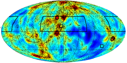
Figure 3.— Left panel: sky maps in equatorial coordinates (RA and DEC) of all halos within a sphere of $20{\>h^{-1}\rm Mpc}$ centered in the MW-like halo in the $\Lambda$CDM simulation for coordinate system $SG_{zero}$. The color scale represents a smoothed mass-weighted count of the number of halos per pixel, going from blue to red for lower to higher counts. The angular positions of all halos with masses larger than $5\times 10^{9}h^{-1}M_{\odot}$ are displayed with black dots. The boxes marked with solid black lines in the center and in the sides are the VdR and aVdR respectively. The locations of the simulated Virgo and Fornax clusters appear as black circles, the correspondent locations of the real clusters appear as black squares. Right panel: same as on the left for coordinate system $SG_{min}$.

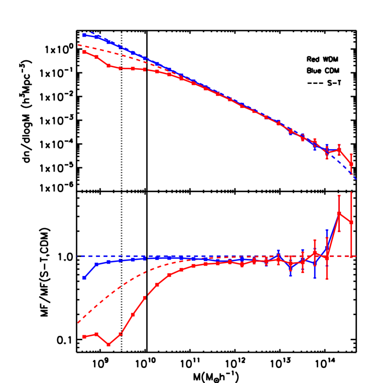
Figure 4.— Upper panel: differential MFs for the $\Lambda$CDM and $\Lambda$WDM constrained simulations (blue and red solid lines respectively). Analytical predictions following the Sheth & Tormen formalism for both cosmologies are shown as dashed lines. Lower panel: ratio of the MFs to the value of the MF given by the Sheth & Tormen formalism for the $\Lambda$CDM cosmology. The solid and dotted vertical lines mark the values of the filtering and limiting mass of the $\Lambda$WDM simulation: $1.1\times 10^{10}h^{-1}$M_⊙ and $3\times 10^{9}h^{-1}$M_⊙ respectively.

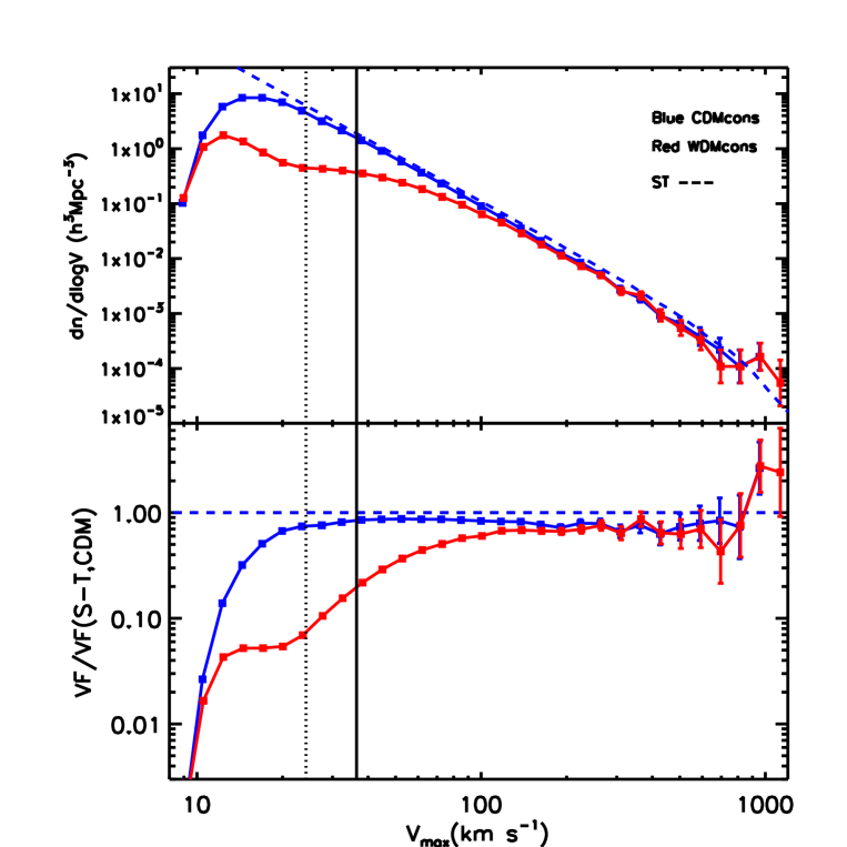
Figure 5.— The same as Fig. 4 but for the VFs instead of the MFs. In this case no analytical prediction is shown for the $\Lambda$WDM cosmology. The vertical lines indicate the maximum velocities corresponding to the filtering and limiting masses, with values of $36\>{\rm km\,s^{-1}}$ and $24\>{\rm km\,s^{-1}}$ respectively.

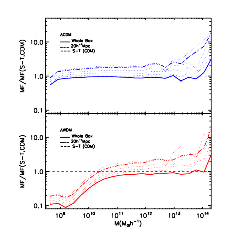
Figure 6.— Ratio of the differential MFs for the $\Lambda$CDM (upper panel) and $\Lambda$WDM (lower panel) CSs to the prediction of the S-T formalism for the $\Lambda$CDM cosmology. The solid lines represent the result for the whole simulation boxes (see Fig. 4). The blue dashed lines are for the S-T prediction. The other lines are for spheres of different radii centered at the LG. The curve for the $20{\>h^{-1}\rm Mpc}$ radius sphere is highlighted with a thick dash-dotted line.

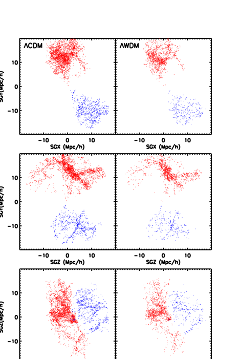
Figure 7.— Projections of the halo distributions in the ALFALFA field of view onto the planes of the supergalactic coordinate system $SG_{min}$. Only halos within $20{\>h^{-1}\rm Mpc}$ from the MW halo and with masses larger than $5\times 10^{9}h^{-1}M_{\odot}$ are shown. The red and blue dots represent halos inside the VdR and aVdR respectively. The left and right panels are for the $\Lambda$CDM and $\Lambda$WDM simulations, respectively.

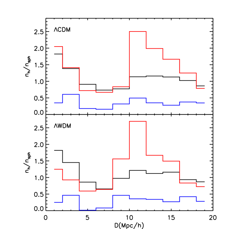
Figure 8.— Upper panel: number density of halos, in the $\Lambda$CDM simulation, as a function of distance to the LG for the halos displayed in Fig. 7. The values are normalized to the number density within the $20{\>h^{-1}\rm Mpc}$ sphere. Red and blue lines are for the VdR and aVdR respectively. The black line gives the radial number density profile for the whole sphere.Lower panel: same as on the left for the $\Lambda$WDM simulation.

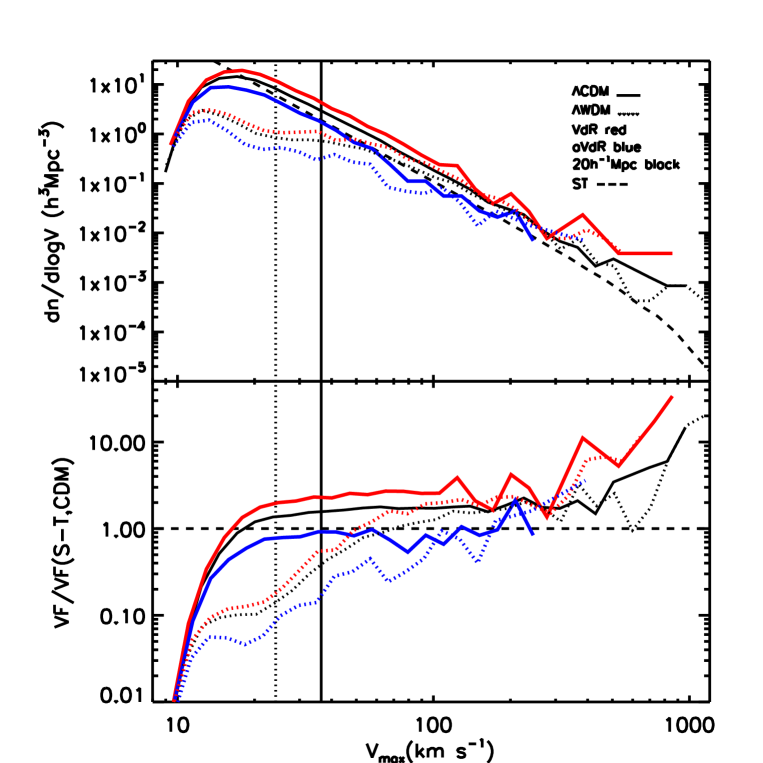
Figure 9.— Upper panel: differential VFs for the $\Lambda$CDM (solid lines) and $\Lambda$WDM (dotted lines) constrained simulations in the VdR (red) and aVdR (blue). The black (solid and dotted) curves are for the sphere of $20{\>h^{-1}\rm Mpc}$ radius centered at the LG. The S-T prediction, only for $\Lambda$CDM cosmology, is shown as a black dashed curve. Lower panel: ratio of the VFs for the simulations to the VF given by the S-T formalism for the $\Lambda$CDM cosmology (same line styles as in the upper panel). The solid and dotted vertical lines mark the values of the filtering and limiting velocities of the $\Lambda$WDM simulation as in previous figures.

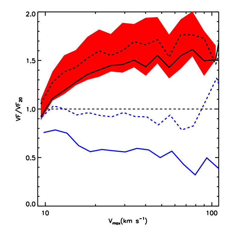
Figure 10.— Ratio of the differential VF of the $\Lambda$CDM simulation for the VdR to the VF in a sphere of $20{\>h^{-1}\rm Mpc}$ radius. The red zone encompasses the value of these ratios for different rotations of the supergalactic coordinate system. The results for two of these rotations, corresponding to the coordinates systems $SG_{zero}$ and $SG_{min}$ defined in section 3, are highlighted as black dashed and solid lines respectively. Also shown are the ratios in the aVdR for these two rotations (blue lines).

Figure 11.— Differential VFs of modeled galaxies (disk+halo). Line-styles and correspondences are as in Fig. 9.

Figure 12.— Upper panel: distribution in equatorial coordinates of the sample of HI sources taken from the ALFALFA public catalogs released so far in the VdR. The position of $M87$ in the Virgo cluster is marked as a red star. Middle panel: sample of sources in the aVdR. Lower panel: the number density of sources as a function of their distance to the MW (red and blue for the VdR and aVdR respectively).

Figure 13.— VF for the sample of galaxies in the VdR taken taken from the ALFALFA catalogs (square symbols with error bars). Predictions from our CSs, using $f_{disk}=0.03$, for the observed field of view appear as the dashed ($\Lambda$CDM) and dotted ($\Lambda$WDM) red areas, delimited by Poisson error bars. The dashed and dotted lines are predictions using a model where $f_{disk}$ is a function of halo mass incorporating the effects of SN feedback. The sensitivity limit of the survey has been included in the results. The vertical solid line marks the value of $V_{max}$ down to which the simulations and observations are both complete.

Figure 14.— The same as Fig. 13 but for the limited survey coverage of the aVdR.

Table 1Main properties of the LG, Virgo and Fornax. The first line is the mass of the object and the second the relative distance to the LG. Distances are given in $h^{-1}$Mpc and masses in $10^{12}h^{-1}$M_⊙.

Object/Case	LG(MW+M31)	Virgo	Fornax
$\Lambda$CDM	$1$	$100$	$27$
	$0.9$	$10.8$	$10.5$
$\Lambda$WDM	$1$	$94$	$31$
	$0.5$	$10.2$	$10.6$
Obs.	1.6	204	31
	0.6	11.4	15.0

References

- Barkana et al. (2001) Barkana, R., Haiman, Z., & Ostriker, J. P. 2001, ApJ, 558, 482
- Benson et al. (2002a) Benson, A. J., Frenk, C. S., Lacey, C. G., Baugh, C. M., & Cole, S. 2002a, MNRAS, 333, 177
- Benson et al. (2002b) Benson, A. J., Lacey, C. G., Baugh, C. M., Cole, S., & Frenk, C. S. 2002b, MNRAS, 333, 156
- Bistolas & Hoffman (1998) Bistolas, V. & Hoffman, Y. 1998, ApJ, 492, 439
- Blanton et al. (2008) Blanton, M. R., Geha, M., & West, A. A. 2008, ApJ, 682, 861
- Blanton & Roweis (2007) Blanton, M. R. & Roweis, S. 2007, AJ, 133, 734
- Bode et al. (2001) Bode, P., Ostriker, J. P., & Turok, N. 2001, ApJ, 556, 93
- Boyarsky et al. (2008a) Boyarsky, A., Lesgourgues, J., Ruchayskiy, O., & Viel, M. 2008a, ArXiv e-prints
- Boyarsky et al. (2008b) Boyarsky, A., Ruchayskiy, O., & Iakubovskyi, D. 2008b, ArXiv e-prints
- Catinella et al. (2006) Catinella, B., Giovanelli, R., & Haynes, M. P. 2006, ApJ, 640, 751
- Catinella et al. (2007) Catinella, B., Haynes, M. P., & Giovanelli, R. 2007, AJ, 134, 334
- Colín et al. (2000) Colín, P., Avila-Reese, V., & Valenzuela, O. 2000, ApJ, 542, 622
- Colín et al. (2008) Colín, P., Valenzuela, O., & Avila-Reese, V. 2008, ApJ, 673, 203
- de Vaucouleurs et al. (1991) de Vaucouleurs, G., de Vaucouleurs, A., Corwin, Jr., H. G., Buta, R. J., Paturel, G., & Fouque, P. 1991, Third Reference Catalogue of Bright Galaxies (Volume 1-3, XII, 2069 pp. 7 figs.. Springer-Verlag Berlin Heidelberg New York)
- Diemand et al. (2007) Diemand, J., Kuhlen, M., & Madau, P. 2007, ApJ, 657, 262
- Diemand et al. (2005) Diemand, J., Moore, B., & Stadel, J. 2005, Nature, 433, 389
- Dutton & van den Bosch (2008) Dutton, A. A. & van den Bosch, F. C. 2008, ArXiv e-prints
- Eke et al. (1998) Eke, V. R., Navarro, J. F., & Frenk, C. S. 1998, ApJ, 503, 569
- Evans & Wilkinson (2000) Evans, N. W. & Wilkinson, M. I. 2000, MNRAS, 316, 929
- Font et al. (2008) Font, A. S., Bower, R. G., McCarthy, I. G., Benson, A. J., Frenk, C. S., Helly, J. C., Lacey, C. G., Baugh, C. M., & et al.,. 2008, MNRAS, 389, 1619
- Gavazzi et al. (2003) Gavazzi, G., Boselli, A., Donati, A., Franzetti, P., & Scodeggio, M. 2003, A&A, 400, 451
- Giovanelli et al. (2005a) Giovanelli, R., Haynes, M. P., Kent, B. R., Perillat, P., Catinella, B., Hoffman, G. L., Momjian, E., Rosenberg, J. L., & et al.,. 2005a, AJ, 130, 2613
- Giovanelli et al. (2005b) Giovanelli, R., Haynes, M. P., Kent, B. R., Perillat, P., Saintonge, A., Brosch, N., Catinella, B., Hoffman, G. L., & et al.,. 2005b, AJ, 130, 2598
- Giovanelli et al. (2007) Giovanelli, R., Haynes, M. P., Kent, B. R., Saintonge, A., Stierwalt, S., Altaf, A., Balonek, T., Brosch, N., & et al.,. 2007, AJ, 133, 2569
- Girardi et al. (1998) Girardi, M., Giuricin, G., Mardirossian, F., Mezzetti, M., & Boschin, W. 1998, ApJ, 505, 74
- Gnedin & Kravtsov (2006) Gnedin, N. Y. & Kravtsov, A. V. 2006, ApJ, 645, 1054
- Gonzalez et al. (2000) Gonzalez, A. H., Williams, K. A., Bullock, J. S., Kolatt, T. S., & Primack, J. R. 2000, ApJ, 528, 145
- Górski et al. (2005) Górski, K. M., Hivon, E., Banday, A. J., Wandelt, B. D., Hansen, F. K., Reinecke, M., & Bartelmann, M. 2005, ApJ, 622, 759
- Hernández-Toledo et al. (2008) Hernández-Toledo, H. M., Vázquez-Mata, J. A., Martínez-Vázquez, L. A., Avila Reese, V., Méndez-Hernández, H., Ortega-Esbrí, S., & Núñez, J. P. M. 2008, AJ, 136, 2115
- Hoeft et al. (2006) Hoeft, M., Yepes, G., Gottlöber, S., & Springel, V. 2006, MNRAS, 371, 401
- Hoffman & Ribak (1991) Hoffman, Y. & Ribak, E. 1991, ApJ, 380, L5
- Jing (2000) Jing, Y. P. 2000, ApJ, 535, 30
- Karachentsev et al. (2004) Karachentsev, I. D., Karachentseva, V. E., Huchtmeier, W. K., & Makarov, D. I. 2004, AJ, 127, 2031
- Kent et al. (2008) Kent, B. R., Giovanelli, R., Haynes, M. P., Martin, A. M., Saintonge, A., Stierwalt, S., Balonek, T. J., Brosch, N., & et al.,. 2008, AJ, 136, 713
- Kilborn et al. (2005) Kilborn, V. A., Koribalski, B. S., Forbes, D. A., Barnes, D. G., & Musgrave, R. C. 2005, MNRAS, 356, 77
- Klypin et al. (2003) Klypin, A., Hoffman, Y., Kravtsov, A. V., & Gottlöber, S. 2003, ApJ, 596, 19
- Klypin et al. (1999) Klypin, A., Kravtsov, A. V., Valenzuela, O., & Prada, F. 1999, ApJ, 522, 82
- Knollmann & Knebe (2009) Knollmann, S. R. & Knebe, A. 2009, ArXiv e-prints
- Komatsu et al. (2008) Komatsu, E., Dunkley, J., Nolta, M. R., Bennett, C. L., Gold, B., Hinshaw, G., Jarosik, N., Larson, D., & et al.,. 2008, ArXiv e-prints
- Koposov et al. (2009) Koposov, S. E., Yoo, J., Rix, H.-W., Weinberg, D. H., Macciò, A. V., & Miralda-Escudé, J. 2009, ArXiv e-prints
- Kravtsov et al. (2002) Kravtsov, A. V., Klypin, A., & Hoffman, Y. 2002, ApJ, 571, 563
- Lahav et al. (2000) Lahav, O., Santiago, B. X., Webster, A. M., Strauss, M. A., Davis, M., Dressler, A., & Huchra, J. P. 2000, MNRAS, 312, 166
- Lukić et al. (2007) Lukić, Z., Heitmann, K., Habib, S., Bashinsky, S., & Ricker, P. M. 2007, ApJ, 671, 1160
- Macciò et al. (2008) Macciò, A. V., Dutton, A. A., & van den Bosch, F. C. 2008, MNRAS, 391, 1940
- Macciò et al. (2005) Macciò, A. V., Governato, F., & Horellou, C. 2005, MNRAS, 359, 941
- Martinez-Vaquero et al. (2007) Martinez-Vaquero, L. A., Yepes, G., & Hoffman, Y. 2007, MNRAS, 378, 1601
- Mathis et al. (2002) Mathis, H., Lemson, G., Springel, V., Kauffmann, G., White, S. D. M., Eldar, A., & Dekel, A. 2002, MNRAS, 333, 739
- Miranda & Macciò (2007) Miranda, M. & Macciò, A. V. 2007, MNRAS, 382, 1225
- Mo et al. (1998) Mo, H. J., Mao, S., & White, S. D. M. 1998, MNRAS, 295, 319
- Moore et al. (1999) Moore, B., Ghigna, S., Governato, F., Lake, G., Quinn, T., Stadel, J., & Tozzi, P. 1999, ApJ, 524, L19
- Peebles (1969) Peebles, P. J. E. 1969, ApJ, 155, 393
- Reed et al. (2007) Reed, D. S., Bower, R., Frenk, C. S., Jenkins, A., & Theuns, T. 2007, MNRAS, 374, 2
- Reiprich & Böhringer (2002) Reiprich, T. H. & Böhringer, H. 2002, ApJ, 567, 716
- Saintonge et al. (2008) Saintonge, A., Giovanelli, R., Haynes, M. P., Hoffman, G. L., Kent, B. R., Martin, A. M., Stierwalt, S., & Brosch, N. 2008, AJ, 135, 588
- Schmidt (1968) Schmidt, M. 1968, ApJ, 151, 393
- Seljak et al. (2006a) Seljak, U., Makarov, A., McDonald, P., & Trac, H. 2006a, Physical Review Letters, 97, 191303
- Seljak et al. (2006b) Seljak, U., Slosar, A., & McDonald, P. 2006b, Journal of Cosmology and Astro-Particle Physics, 10, 14
- Sheth et al. (2001) Sheth, R. K., Mo, H. J., & Tormen, G. 2001, MNRAS, 323, 1
- Sheth & Tormen (1999) Sheth, R. K. & Tormen, G. 1999, MNRAS, 308, 119
- Sheth & Tormen (2002) —. 2002, MNRAS, 329, 61
- Sigad et al. (2000) Sigad, Y., Kolatt, T. S., Bullock, J. S., Kravtsov, A. V., Klypin, A. A., Primack, J. R., & Dekel, A. 2000, ArXiv Astrophysics e-prints
- Solanes et al. (2001) Solanes, J. M., Manrique, A., García-Gómez, C., González-Casado, G., Giovanelli, R., & Haynes, M. P. 2001, ApJ, 548, 97
- Somerville (2002) Somerville, R. S. 2002, ApJ, 572, L23
- Spergel et al. (2007) Spergel, D. N., Bean, R., Doré, O., Nolta, M. R., Bennett, C. L., Dunkley, J., Hinshaw, G., Jarosik, N., & et al.,. 2007, ApJS, 170, 377
- Springel (2005) Springel, V. 2005, MNRAS, 364, 1105
- Springel et al. (2008) Springel, V., Wang, J., Vogelsberger, M., Ludlow, A., Jenkins, A., Helmi, A., Navarro, J. F., Frenk, C. S., & et al.,. 2008, MNRAS, 391, 1685
- Springob et al. (2005) Springob, C. M., Haynes, M. P., Giovanelli, R., & Kent, B. R. 2005, ApJS, 160, 149
- Steffen (2006) Steffen, F. D. 2006, Journal of Cosmology and Astro-Particle Physics, 9, 1
- Sulentic et al. (2006) Sulentic, J. W., Verdes-Montenegro, L., Bergond, G., Lisenfeld, U., Durbala, A., Espada, D., Garcia, E., Leon, S., & et al.,. 2006, A&A, 449, 937
- Swaters et al. (2009) Swaters, R. A., Sancisi, R., van Albada, T. S., & van der Hulst, J. M. 2009, A&A, 493, 871
- Tikhonov & Klypin (2009) Tikhonov, A. & Klypin, A. 2009, MNRAS in print
- Tonry et al. (2000) Tonry, J. L., Blakeslee, J. P., Ajhar, E. A., & Dressler, A. 2000, ApJ, 530, 625
- Tonry et al. (2001) Tonry, J. L., Dressler, A., Blakeslee, J. P., Ajhar, E. A., Fletcher, A. B., Luppino, G. A., Metzger, M. R., & Moore, C. B. 2001, ApJ, 546, 681
- Tully et al. (2009) Tully, R., Rizzi, L., Shaya, E., Courtois, H., Makarov, D., & Jacobs, B. 2009, ArXiv e-prints
- Verheijen & Sancisi (2001) Verheijen, M. A. W. & Sancisi, R. 2001, A&A, 370, 765
- Viel et al. (2005) Viel, M., Lesgourgues, J., Haehnelt, M. G., Matarrese, S., & Riotto, A. 2005, Phys. Rev. D, 71, 063534
- Viel et al. (2006) —. 2006, Physical Review Letters, 97, 071301
- Wang & White (2007) Wang, J. & White, S. D. M. 2007, MNRAS, 380, 93
- Wang et al. (2007) Wang, L., Li, C., Kauffmann, G., & De Lucia, G. 2007, MNRAS, 377, 1419
- Weinmann et al. (2006) Weinmann, S. M., van den Bosch, F. C., Yang, X., Mo, H. J., Croton, D. J., & Moore, B. 2006, MNRAS, 372, 1161
- Willick et al. (1997) Willick, J. A., Courteau, S., Faber, S. M., Burstein, D., Dekel, A., & Strauss, M. A. 1997, ApJS, 109, 333
- Xue et al. (2008) Xue, X. X., Rix, H. W., Zhao, G., Re Fiorentin, P., Naab, T., Steinmetz, M., van den Bosch, F. C., Beers, T. C., & et al.,. 2008, ApJ, 684, 1143
- Zaroubi et al. (1999) Zaroubi, S., Hoffman, Y., & Dekel, A. 1999, ApJ, 520, 413
- Zavala (2003) Zavala, J. 2003, The luminous and baryonic fundamental plane of disk galaxies. B.Sc. Thesis
- Zavala et al. (2008) Zavala, J., Okamoto, T., & Frenk, C. S. 2008, MNRAS, 387, 364
- Zheng et al. (2007) Zheng, Z., Coil, A. L., & Zehavi, I. 2007, ApJ, 667, 760