Dynamically Slow Processes in Supercooled Water Confined Between Hydrophobic Plates

Abstract

We study the dynamics of water confined between hydrophobic flat surfaces at low temperature. At different pressures, we observe different behaviors that we understand in terms of the hydrogen bonds dynamics. At high pressure, the formation of the open structure of the hydrogen bond network is inhibited and the surfaces can be rapidly dehydrated by decreasing the temperature. At lower pressure the rapid ordering of the hydrogen bonds generates heterogeneities that are responsible for strong non-exponential behavior of the correlation function, but with no strong increase of the correlation time. At very low pressures, the gradual formation of the hydrogen bond network is responsible for the large increase of the correlation time and, eventually, the dynamical arrest of the system and of the dehydration process.

1 Introduction

1.1 Supercooled Water and Polyamorphism

Supercooled water is a metastable state of the liquid water with respect to the crystal ice and occurs when H₂O is cooled slowly below the freezing point. It can be easily prepared by cooling relatively pure commercial water and is commonly observed in nature, especially under confinement as for example in plants where water is still liquid at $-47^{o}$C. It may crystallize into ice by catalysts, such as an ice crystal, or by a large exchange of mechanical energy, such as a strong vibration. However, without catalysts or external work, it is a useful example of a liquid whose dynamics slows down when the temperature decreases toward the homogeneous nucleation temperature $T_{H}$ (with $T_{H}=-41^{o}$C at 1 atm and $T_{H}=-92^{o}$C at 2000 atm) [1]. The study of supercooled water is important in the long-lasting efforts to understand the physics of the hydrogen bonds, which characterize water and are the origin of its unique properties [2].

Below $T_{H}$ water crystallizes, but a fast quench from ambient $T$ to $T<T_{X}=-123^{o}$C (at 1 atm) freezes the liquid into a disordered (not crystalline) ice, leading to the formation of (amorphous) glassy water [3]. By increasing the pressure it has been observed that glassy water changes from low density amorphous (LDA) to high density amorphous (HDA) [4] and from HDA to very-high density amorphous (VHDA) [5]. Therefore, water shows polyamorphism and this phenomenon has been related to the possible existence of more than one liquid phase of water [6]. Other thermodynamically consistent scenarios have been proposed, such as a first-order liquid-liquid phase transition with no critical point [7] or the absence of liquid-liquid phase transition itself [8], and their experimental implications are currently debated [9].

1.2 Confined Water

Confinement is an effective way to suppress the crystal nucleation. Water molecules in plants, rocks, carbon nanotubes, living cells or on the surface of a protein, are confined to the nanometer scale. Many recent experiments show a rich phenomenology which is the object of an intense debate (see for example [10, 11, 12, 13, 7, 14, 15, 16, 17, 18, 19]). The relation between the properties of confined and bulk supercooled water is not fully understood, therefore it is useful to elaborate handleable models that could help in developing a consistent theory.

1.3 Models for Water

Since the experiments in the supercooled region are difficult to perform, numerical simulations are playing an important role in the interpretation of the data. These simulations are based on models with different degree of detailed description and complexity. Among the most commonly used, there are the ST2 [20] (two positive and two negative charges in tetrahedral position plus a central Lennard-Jones or LJ), the SPC and its modification SPC/E (three negative and one positive charges plus a central LJ) [21], the TIP3P, TIP4P, and TIP5P with three, four and five charges, respectively [22], the models with internal degrees of freedom [23], polarizability and three body interactions [24], and ab initio models for the evaluation of the significance of quantum effects [25].

Models with increasing details lead to improved accuracy in the simulations, but suffer from important technical limitations in time and size of the computation. Due to their complexity, an analysis of how each of their internal parameter affects the properties of the model is in general very computationally expensive and a theoretical prediction of their behavior is unfeasible, limiting their capacity to offer an insight into unifying concepts in terms of universal principles and hampering their ability to study thermodynamics properties.

On the other hand, simplified theoretical models, such as the Ising model, can be very drastic in their approximations, but are able to offer a general view on global, and possibly universal, issues such as thermodynamics and dynamics. They can be studied analytically or by simulations, providing theoretical predictions that can be tested by numerical computation. Therefore, they offer a complementary approach to the direct simulation of detailed models. Their characterization in terms of few internal parameters make them more flexible and versatile, offering unifying views of different cases. Their study by theoretical methods, such as mean field, leads to analytic functional relations for their properties, allowing to predict their behavior over all the possible values of the external parameters. Their reduced computational cost permits direct test of the theoretical forecasts in any condition. Furthermore, their study helps in defining improved detailed models for greater computational efficiency. Therefore, there is a strong need for simplified models of water that can keep the physical information and provide a more efficient simulation tool.

In the following we will describe a simple model for water in two dimensions (2D). The model can be easily extended to 3D, however we consider here only the 2D case. It can be thought as a monolayer of water between two flat hydrophobic plates where the water-wall interaction is purely repulsive (steric hard-core exclusion). It has been shown that the properties of confined water are only weakly dependent on the details of the confining potential between smooth walls and that the plate separation is the relevant parameter determining whether or not a crystal forms [26]. The case we consider here corresponds to the physical situation in which the distance between the plates inhibits the crystallization.

2 Cooperative Cell Model Confined Between Partially Hydrated Hydrophobic Plates

2.1 General Definition of the Model

Cell models with variable volume are particularly suitable to describe fluids at constant pressure $P$, temperature $T$ and number of molecules $N$ as in the majority of experiments with water. Here we consider a cell model based on the idea of including a three-body interaction, as well as an isotropic and a directional term for the hydrogen bonds [27, 28]. The three-body term takes into account the cooperative nature of the hydrogen bond. This model reproduces the experimental phase diagram of liquid water [29, 30] and, by varying its parameters, the different scenarios for the anomalies of water [31, 32].

We consider water confined between two hydrophobic plates within a volume $V$ that accommodates $N$ molecules. To minimize the boundary effects, we consider double periodic conditions. We assume that the distance between the plates is such that water forms a monolayer on a square surface, similar to the one observed in molecular dynamics simulations for TIP5P water, where each water molecule has four nearest neighbors [33]. The system is divided into $L^{2}$ cells of equal volume $v=V/L^{2}$. Differently from previous works on this model [34, 27, 35, 29, 28, 9, 2, 30, 31, 32], here we consider partially hydrated walls with a hydration level corresponding to a water concentration of 75% with respect to the available surface of one wall. This concentration is well above the site percolation threshold (59.3%) on a square lattice [36]. We assume that in each cell $i=1,2,\ldots L^{2}$ there is at most one water molecule and we assign the variable $n_{i}=1$ if the cell is occupied, and $n_{i}=0$ otherwise.

The water-water interaction is described by three terms. One takes into account all the isotropic contributions (short-range repulsion of the electron clouds, weak attractive van der Waals or London dispersion interaction, strong attractive isotropic component of the hydrogen bond interaction). This term is given by a hard-core repulsive at distance volume $R_{0}=v_{0}^{1/2}$ plus a LJ potential

$$U(r)=\left\{\begin{array}[]{lll}\infty&{\rm for}&\ r\leq R_{0}\\ \displaystyle\epsilon\left[\left(\frac{R_{0}}{r}\right)^{12}-\left(\frac{R_{0}}{r}\right)^{6}\right]&{\rm for}&\ r>R_{0},\end{array}\right.$$ (1)

where $r$ is the distance between two molecules.

The second term takes into account the directionality of the hydrogen bonds interaction. Each molecule participates in at most four hydrogen bonds when each donor O-H forms an angle with the acceptor O that deviates from linear (180^o) within 30^o or 40^o approximately. To incorporate this feature to the model, we associate to each water molecule $i$ four indices $\sigma_{ij}\in[1,2,\ldots q]$, one for each possible hydrogen bond with the nearest neighbors molecules $j$. The parameter $q$ is chosen by selecting 30^o as maximum deviation from the linear bond, hence $q=180/30\equiv 6$. With this choice, every molecule has $q^{4}=6^{4}\equiv 1296$ possible orientations. This directional interaction can be accounted for by the energy term

$$E_{J}=-J\sum_{\langle i,j\rangle}n_{i}n_{j}\delta_{\sigma_{ij},\sigma_{ji}}=-JN_{HB},$$ (2)

where the sum runs over all nearest-neighbor cells, $J>0$ is the energy associated to the formation of a hydrogen bond, and $N_{HB}$ is the total number of hydrogen bonds in the system.

As a consequence of their directionality, the hydrogen bonds induce a rearrangement of the molecules in an open network (tetrahedral in 3D), in contrast with the more dense arrangement that can be observed at higher $T$ or higher $P$ [37]. This effect can be included in the model by associating a small volume contribution $v_{HB}$, due to the formation of each bond, to the total volume of the system

$$V=V_{0}+N_{HB}v_{HB}$$ (3)

where $V_{0}=Nv_{0}$ is the volume of the liquid with no hydrogen bonds.

Finally, experiments show that the relative orientations of the hydrogen bonds of a water molecule are correlated [38]. As an effect of the cooperativity between the hydrogen bonds, the O–O–O angle distribution becomes sharper at lower $T$ [11]. Therefore, the accessible $q$ values are reduced. We include this effect in the model by the energy term

$$E_{\sigma}=-J_{\sigma}\sum_{i}n_{i}\sum_{(k,l)_{i}}\delta_{\sigma_{ik},\sigma_{il}},$$ (4)

where $J_{\sigma}$ is the energy gain due to the cooperative ordering of the hydrogen bonds, $(k,l)_{i}$ stands for the 6 different pairs of bond indices (arms) of a molecule $i$. At low $T$ this terms induces the reduction of accessible values of $q$ (orientational ordering). In the limiting case $J_{\sigma}=0$ there is no correlation between bonds [8]. This case corresponds to consider as negligible the observed change in O–O–O angle distribution with $T$. The case $J_{\sigma}\gg 1$ corresponds to a drastic reduction of orientational states for the molecule from $q^{4}$ to $q$, with all the relative orientation between the hydrogen bonds kept fixed independently from $T$ and $P$.

2.2 The Parameters Dependence of Phase Diagram of the Model

The complete enthalpy for the fluid reads

$$H=U(r)+E_{J}+E_{\sigma}+PV.$$ (5)

Each of the energy terms of (5) provides an energy scale, and depending on their relative importance different physical situations emerge. For instance, the choice $J<\epsilon$ guarantees that the hydrogen bonds are mainly formed in the liquid phase. As showed in [32], when $J_{\sigma}=0$ the model gives rise to the scenario with no liquid-liquid coexistence [8]; at larger $J_{\sigma}/J$ the model displays the scenario with a liquid-liquid critical point at positive pressure [6]; further increase of $J_{\sigma}/J$ brings to a liquid-liquid critical point at negative pressure [39]; finally more increase of $J_{\sigma}/J$ brings to the scenario where the liquid-liquid phase transition extends to the negative pressure of the limit of stability of the liquid phase [7].

The term

$$E_{J}+PV\equiv-(J-Pv_{HB})N_{HB}+PV_{0}$$ (6)

is proportional to the number of hydrogen bonds $N_{HB}$ and the associated gain in enthalpy decreases linearly with increasing pressure, being maximum at the lowest accessible $P$ for the liquid, and being zero at $P=J/v_{HB}$. For $P>J/v_{HB}$ the formation of hydrogen bonds increases the total enthalpy.

In the following we choose $J/\epsilon=0.5$, $J_{\sigma}/\epsilon=0.05$, $v_{HB}/v_{0}=0.5$ as in Ref. [29], for sake of comparison. In the next sections we describe the simulation method adopted here and the results.

3 Kawasaki Monte Carlo Method

Monte Carlo (MC) simulations are performed in the ensemble with constant $N$, $P$, $T$ for $N=1875$ water molecules distributed in a mesh of $L^{2}=2500$ cells, corresponding to 75% water concentration. We do not observe appreciable size effects at constant water concentration for ($N=300$, $L^{2}=400$) and ($N=1200$, $L^{2}=1600$). Preliminary results at 90% water concentration display no significant differences with the present case.

Since we are interested in studying the dynamic behavior of the system when diffusion is allowed, we adopt a MC method a la Kawasaki [40]. This method consists in exchanging the content of two stochastically selected nearest neighbors (n. n.) cells and accepting the exchange with probability

$$\left\{\begin{array}[]{ll}\exp[-\Delta H/k_{B}T]&{\rm if}\ \Delta H>0\cr 1&{\rm if}\ \Delta H<0\cr\end{array}\right.$$ (7)

where $\Delta H$ is the difference between the enthalpy of the final state and that of the initial state.

The same probability is adopted for every attempt to change the state of any of the bond indices $\sigma_{ij}$. One MC step consists of $5N$ trials of exchanging n. n. cells $i$ and $j$ or changing the state of the bond indices $\sigma_{ij}$ (every time selecting at random which kind of move and which $i$ and $j$ are considered) followed by a volume change attempt. In the latter case, the new volume is selected at random in the interval $[V-\delta V,V+\delta V]$ with $\delta V=0.5v_{0}$.

For sake of simplicity, in the Lennard-Jones energy calculation we do not consider the volume changes due to the hydrogen bonds formation and we allow the formation of hydrogen bonds independently from the size of the n. n. cells. We include a cut-off for the Lennard-Jones interaction at a distance equal to three times the size of a cell. Despite with this choice the cut-off is density dependent, we tested that in this way we largely reduce the computational cost and that the results do not change in a significant way with respect to the case without the cut-off.

In the simulations we follow an annealing protocol, by preparing a random configuration and equilibrating it at high $T$ and low $P$ (gas phase). We equilibrate the system over $5\times 10^{5}$ MC steps, and calculate the observable averaging over at least $2\times 10^{6}$ MC steps. We use the final equilibrium configuration at a given temperature as the starting configuration for the next lower temperature.

4 Results and Discussion

4.1 The Phase Diagram

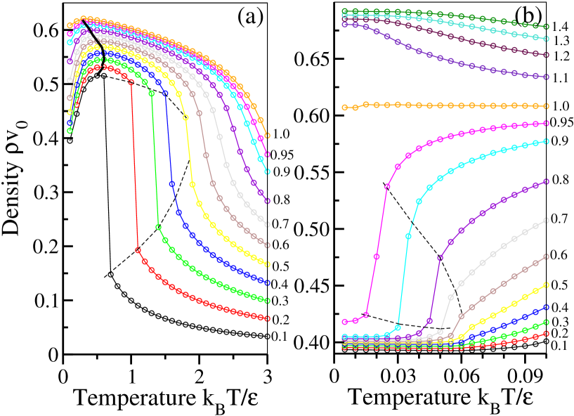
Figure 1: Density $\rho$ of fluid water as function of temperature $T$ at different values of pressure $P$. (a) At high $T$ a discontinuity in $\rho$ appears below $Pv_{0}/\epsilon=0.5$, marking the first order phase transition between gas (at low $\rho$) and liquid (at high $\rho$), ending in a critical point at approximately $k_{B}T_{C}/\epsilon=1.9\pm 0.1$, $P_{C}v_{0}/\epsilon=0.50\pm 0.05$. In the liquid phase, isobars show a temperature of maximum density (TMD line, marked by the thick black line) one of the characteristic features of water. (b) At low $T$ the density rapidly decreases for $P<J/v_{HB}=1\epsilon/v_{0}$ with a discontinuity marking the first order phase transition between high density liquid (at high $\rho$) and low density liquid (at low $\rho$), ending in a critical point at approximately $k_{B}T_{C^{\prime}}/\epsilon=0.06\pm 0.01$, $P_{C^{\prime}}v_{0}/\epsilon=0.60\pm 0.15$. In both panels, symbols are results of the MC calculation, lines are guides for the eyes, errors are comparable to the size of the symbols, labels on the right of each panel are the values of $Pv_{0}/\epsilon$ of the nearest curve.

From the calculation of the density of the system at fixed $P$ as function of $T$ we find a liquid-gas first order phase transition ending in a critical point $C$ at approximately $k_{B}T_{C}/\epsilon=1.9\pm 0.1$, $P_{C}v_{0}/\epsilon=0.50\pm 0.05$ (Fig. 1a). In the liquid phase, we observe a temperature of maximum density (TMD) for any isobar with $Pv_{0}/\epsilon\leq 1$. This anomalous behavior in density is one of the characteristic features of water. Here we note that $Pv_{0}/\epsilon\leq 1$ corresponds to the limiting value $P=J/v_{HB}$ above which the formation of bonds increases the enthalpy in Eq.(6), consistent with the intuitive idea that the density maximum in water is a consequence of the open structure due to the hydrogen bond formation. For $P>J/v_{HB}$ the formation of hydrogen bonds is no longer convenient in terms of free energy and the system recovers the behavior of a normal liquid (with no open structures).

At lower $T$ and for $P\leq J/v_{HB}=1\epsilon/v_{0}$, the isobars display another discontinuity between high density and low density (Fig.1b), both at $\rho$ higher than the gas density. As in the case with no diffusion [29], we associate this discontinuity in $\rho$ to a first order phase transition between a high density liquid (HDL) and a low density liquid (LDL) ending in critical point $C^{\prime}$ at $k_{B}T_{C^{\prime}}/\epsilon=0.06\pm 0.01$ and $P_{C^{\prime}}v_{0}/\epsilon=0.60\pm 0.15$. The values of the critical temperature and pressure for $C$ and the critical temperature for $C^{\prime}$ are consistent, within the error bars, to those previously estimated [29, 28], while the value of $P_{c^{\prime}}$ is somehow smaller. This is due to the difficulty in estimating the position of $C^{\prime}$ from the discontinuity of $\rho$ and it will be discussed in a future work. Here, instead, we focus on the analysis of the dynamics of the system at low $T$.

4.2 The Dynamics at Low Temperature

To get an insight into the processes at low $T$ associated with the hydrogen bond dynamics, we calculate the the quantity $M_{i}\equiv\frac{1}{4}\sum_{j}\sigma_{ij}$, that gives the orientational order of the four bond indices of molecule $i$, and its correlation function

$$C_{M}(t)\equiv\frac{1}{N}\sum_{i}\frac{\langle M_{i}(t_{0}+t)M_{i}(t_{0})\rangle-\langle M_{i}\rangle^{2}}{\langle M_{i}^{2}\rangle-\langle M_{i}\rangle^{2}}$$ (8)

where the $\langle\cdot\rangle$ stands for the thermodynamic average [30, 31].

As we have discussed in the previous section, the effect of the hydrogen bond is evident only at pressure $P\leq J/v_{HB}$ and below the TMD line. Therefore we focus on state points at $P\leq 1\epsilon/v_{0}$ and $T\leq 0.4\epsilon/k_{B}$.

• We first observe that for $P=1\epsilon/v_{0}$ the correlation function is always exponential for all the temperatures with $0.005\leq k_{B}T/\epsilon\leq 0.4$ (Triangles in Fig.2). From the exponential fits (dotted lines in Fig.2) the characteristic decay time is $\tau\simeq 1.3$ MC Steps (MCS) at $k_{B}T/\epsilon=0.4$ (green symbols), $\tau\simeq 2.2$ MCS at $k_{B}T/\epsilon=0.1$ (red symbols), $\tau\simeq 10$ MCS at $k_{B}T/\epsilon=0.05$ (black symbols). Therefore, the correlation time increases of one order of magnitude for a decrease of $T$ of one order of magnitude, but $\tau$ is always much shorter than the simulation time.

  This behavior is consistent with the observation of the typical configurations of hydrogen bonds at these $P$ and $T$ (upper row in Fig. 3). The water molecules condense on the hydrophobic surface, leaving a large dehydrated area, but the number of hydrogen bonds does not increase in an evident way and no orientational order is observed even at the lowest $T$.

• Next we decrease the pressure to $P=0.7\epsilon/v_{0}$ (Diamonds in Fig.2), close to the the liquid-liquid critical pressure. At $k_{B}T/\epsilon=0.4$ (green symbols), the correlation function is exponential with $\tau\simeq 1$ MCS. At lower $T$ the correlation function is no longer exponential. It can be well described with a stretched exponential function

  $$C_{M}(t)=C_{0}\exp\left[-\left(t/\tau\right)^{\beta}\right]$$ (9)

  where $C_{0}$, $\tau$ and $\beta\leq 1$ are fitting constant. For $\beta=1$ the function is exponential, and the more stretched is the function, the smaller is the power $0<\beta\leq 1$.

  At $k_{B}T/\epsilon=0.1$ (red symbols), the stretched exponential (continuous red line) has $\beta=0.8$ and $\tau\simeq 3.1$ MCS, while at $k_{B}T/\epsilon=0.05$ (black symbols), the stretched exponential (continuous black line) has $\beta=0.4$ and $\tau\simeq 5$ MCS.

  Hence, along isobars close to the liquid-liquid critical pressure, the dynamics of the liquid is not much slower than that at $Pv_{0}/\epsilon=1$, but it becomes non exponential below the TMD, a typical precursor phenomenon of glassy systems [41]. This phenomenology is usually associated with the presence of heterogeneity in the system. While in a homogeneous system the characteristic relaxation time is determined by some characteristic energy scale, in a heterogeneous system the presence of many characteristic energies induces the occurrence of many typical time scales, giving rise to a non exponential behavior.

  This is consistent with the increasing number of hydrogen bonds that can be observed at this pressure in the high density liquid phase (central panel on the second row in Fig. 3). The formation of many hydrogen bonds inhibits the free diffusion of the molecules, determining heterogeneities.

  This effect is extremely evident at the lower $k_{B}T/\epsilon=0.05$, where the non exponential behavior of the correlation function is very strong ($\beta=0.4$) and the hydrogen bond network is fully developed, but with many isolated locally disordered regions (left panel on the second row in Fig. 3). This is the typical configuration of the hydrophobic surface at low $T$ at this $P$. The surface is partially hydrated by low density liquid water forming an open network of bonded molecules. The network is almost complete, but many small heterogeneities are present.

• By further decreasing the pressure to $P=0.4\epsilon/v_{0}$ (Squares in Fig.2), we observe an exponential decay of the correlation function at $k_{B}T/\epsilon=0.4$ (dotted line) with $\tau\simeq 1.3$ MCS and a stretched exponential behavior when the liquid-liquid critical temperature is approached. Differently from the case at $P=0.7\epsilon/v_{0}$, at $P=0.4\epsilon/v_{0}$ the stretched exponent does not decrease in a strong way, but the relaxation time largely increases at lower $T$.

  In particular, at $k_{B}T/\epsilon=0.1$ (red symbols), the stretched exponential (dashed red line) has $\beta=0.9$ and $\tau\simeq 18$ MCS, while at $k_{B}T/\epsilon=0.05$ (black symbols), the stretched exponential (dashed black line) has $\beta=0.7$ and $\tau\simeq 100$ MCS. Therefore, the correlation time slows down of two order of magnitudes by decreasing the $T$ from $k_{B}T/\epsilon=0.4$ to $k_{B}T/\epsilon=0.05$.

  This different behavior with respect to the case at $P=0.7\epsilon/v_{0}$ could be associated to the different evolution of the hydrogen bond network. Previous mean field [28] and MC results [2] have shown that the increase of the number of hydrogen bonds with decreasing $T$ is much more gradual at low $P$ than at high $P$. Therefore, at high $P$ this process could generate quenched-in heterogeneities and strong non-exponentiality. At low $P$, instead, the gradual building up of the hydrogen bond network freezes the system, inducing a large slowing down. As a consequence, the systems has large relaxation times, but the hydrogen bond network develops in a more ordered way (third row in Fig. 3).

  The gradual increase of the number of hydrogen bonds is also responsible for the slower dehydration of the hydrophobic surface. Many small dehydrated regions seem to be annealed at a very slow rate by the progressive network formation.

• We finally consider the lowest pressure $P=0.1\epsilon/v_{0}$ (Circles in Fig.2). In this case, the correlation time is exponential for $k_{B}T/\epsilon=0.4$ (dotted green line) and $k_{B}T/\epsilon=0.1$ (dotted red line), with $\tau\simeq 1.3$ MCS and $\tau\simeq 2.2$ MCS, respectively.

  At these temperatures the system is homogeneous, with no order at $k_{B}T/\epsilon=0.4$ (right panel on the bottom row in Fig. 3) and with small orientationally ordered regions at $k_{B}T/\epsilon=0.1$ (central panel on the bottom row in Fig. 3). These regions are the effect of the slowly increasing number of hydrogen bonds $N_{HB}$ and are possible only at low $P$, because only at low values of $P$ the enthalpy increase proportional to $N_{HB}$ [Eq.(6)] is small.

  As a consequence of the gradual increase of these locally ordered regions of bonded molecules, at lower $T$ the system is trapped in a metastable excited state where large regions of ordered bonded molecules, with different orientations, compete in their growth process (left panel on the bottom row in Fig. 3). These process resembles the arrested dynamics of other model systems for glassy dynamics [42]. It is characterized by non exponential correlation behavior with characteristic times that are several order of magnitudes larger than those at slightly higher $T$. In our case the correlation time largely exceeds the simulation time of $10^{6}$ MCS (Full Circles in Fig. 2).

5 Conclusions

We have studied the dynamics of the hydrogen bond network of a monolayer of water between hydrophobic plates at partial hydration. We adopt a model for water with cooperative interactions [35, 27, 43]. The model can reproduce the different scenarios proposed for water [32]. We consider the parameters that give rise to a liquid-liquid phase transition ending in a critical point [29, 28]. It has been shown that in the supercooled regime, below the TMD line, the system has slow dynamics [30, 2, 31]. Here we adopt a diffusive MC dynamics to study the case at partial hydration.

Our results show a complex phenomenology. At high $P$ the effect of the hydrogen bond network is negligible due to the high increase of enthalpy for the hydrogen bond formation. This is reflected in the dynamics by a moderate increase of the correlation time also at very low $T$. Therefore, the system reaches the equilibrium easily. As a consequence, we typically observe the formation of a single large dehydrated region.

At a pressure close to the liquid-liquid critical pressure, the rapid formation of the hydrogen bond network determines the presence of large amount of heterogeneity in the system. As a consequence the correlation function shows a strong non-exponential behavior at low $T$, where we typically observe a well developed hydrogen bond network with many local heterogeneities. Nevertheless, the hydrogen bond network is fully developed only at very low $T$, keeping the correlation time short and allowing the formation of large dehydrated regions on the hydrophobic surface.

At lower $P$, the number of hydrogen bonds grows in a gradual and more homogeneous way when the temperature decreases. This process slows down the correlation decay of orders of magnitudes. Nevertheless, the effect on the exponential character of the correlation function is small, because the system has only a small amount of heterogeneity. However, the effect on the process of dehydration of the surface is evident.

This effect is extremely strong at very low $P$, where regions of ordered bonded molecules with different orientation grow in a competing fashion. This process give rise to an arrested dynamics, typical of many glassy systems, with the correlation time that increases of many orders of magnitude for a small decrease in temperature. The dehydration process in this case is almost completely frozen on the time scale of our simulations.

References

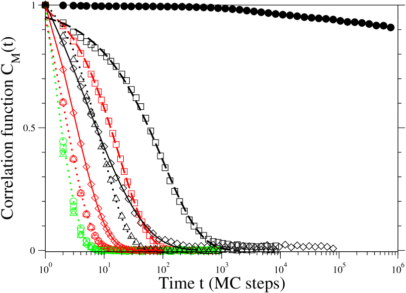
Figure 2: The correlation function $C_{M}(t)$ for different pressure and temperature below the temperature of maximum density (TMD). The correlation decays as an exponential (dotted lines) at any $T\geq 0.4\epsilon/k_{B}$, just below the TMD, for any $P<1.0\epsilon/v_{0}$ (green symbols) and for all $T$ at $P=1\epsilon/v_{0}$ (Triangles). The correlation $C_{M}(t)$ is well described by a stretched exponential (see text) for $P=0.7\epsilon/v_{0}$ (Diamonds) and $P=0.4\epsilon/v_{0}$ (Squares) for $T\leq 0.1\epsilon/k_{B}$ with a stretched exponent $\beta$ that is larger at lower $T$. At low pressure $P=0.1\epsilon/v_{0}$ (Circles), $C_{M}(t)$ is non-exponential only at very low $T=0.05\epsilon/k_{B}$ (full Circles).

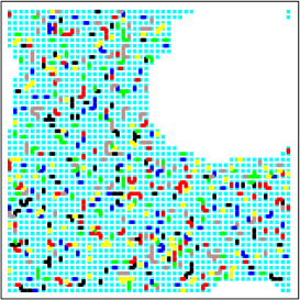
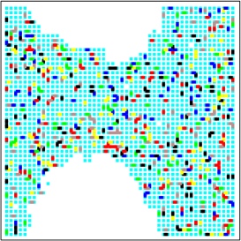
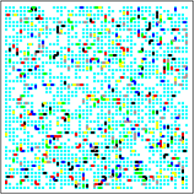
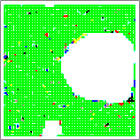
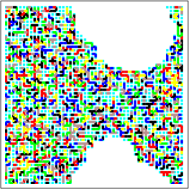
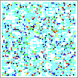
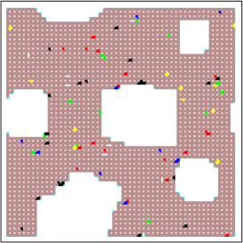
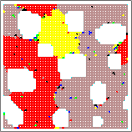
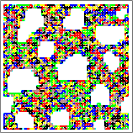
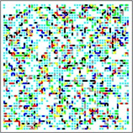
Figure 3: Hydrogen bonds configurations showing the hydrogen bond ordering at low $T$ and at $P<J/v_{HB}=1\epsilon/v_{HB}$. Symbols: Turquoise dots represent cells containing water molecules with at least one bond free; colored lines represent hydrogen bonds between molecules in n. n. cells, with six possible colors corresponding to the $q=6$ possible values of the orientational state. Every row corresponds to a different $P$: from top, $P=1\epsilon/v_{0}$, $P=0.7\epsilon/v_{0}$, $P=0.4\epsilon/v_{0}$, $P=0.1\epsilon/v_{0}$. Every column corresponds to a different $T$: from right, $T=0.4\epsilon/k_{B}$, $T=0.1\epsilon/k_{B}$, $T=0.05\epsilon/k_{B}$. The size of the box is not in scale with the total volume of the system at the different values of $P$ and $T$.

References

- [1] Debenedetti P G and Stanley H E 2003 Physics Today 56 40–46
- [2] Kumar P, Franzese G and Stanley H E 2008 Journal of Physics: Condensed Matter 20 244114
- [3] Loerting T and Giovambattista N 2006 Journal of Physics: Condensed Matter 18 R919–R977
- [4] Mishima O, Calvert L and Whalley E 1985 Nature 314 76–78
- [5] Loerting T, Salzmann C, Kohl I, Mayer E and Hallbrucker A 2001 Physical Chemistry Chemical Physics 3 5355–5357
- [6] Poole P, Sciortino F, Essmann U and Stanley H 1992 Nature 360 324–328
- [7] Angell C A 2008 Science 319 582–587
- [8] Sastry S, Debenedetti P G, Sciortino F and Stanley H E 1996 Physical Review E 53 6144–6154
- [9] Franzese G, Stokely K, Chu X Q, Kumar P, Mazza M G, Chen S H and Stanley H E 2008 Journal of Physics: Condensed Matter 20 494210
- [10] Faraone A, Liu K H, Mou C Y, Zhang Y and Chen S H 2009 Journal of Chemical Physics 130 134512
- [11] Ricci M A, Bruni F and Giuliani A 2009 Faraday Discussussion 141 347-358
- [12] Soper A K 2008 Molecular Physics 106 2053 – 2076
- [13] Bellissent-Funel M C 2008 Journal of Physics: Condensed Matter 20 244120
- [14] Giovambattista N, Lopez C F, Rossky P J and Debenedetti P G 2008 Proceeding of the National Academy of Science of the United States of America 105 2274–2279
- [15] Vogel M 2008 Physical Review Letters 101 181801
- [16] Pawlus S, Khodadadi S and Sokolov A P 2008 Physical Review Letters 100 108103
- [17] Gallo P and Rovere M 2007 Physical Review E 76 061202–7
- [18] Mallamace F, Branca C, Broccio M, Corsaro C, Mou C Y and Chen S H 2007 Proceedings of the National Academy of Sciences 104 18387–18391
- [19] Chen S H, Liu L, Fratini E, Baglioni P, Faraone A and Mamontov E 2006 Proceeding of the National Academy of Science of the United States of America 103 9012–9016
- [20] Stillinger F and A R 1974 Journal of Chemical Physics 60 1545
- [21] Berendsen H, Grigera J and Straatsma T 1987 Journal of Physical Chemistry 91 6269–6271
- [22] Jorgensen W, Chandrasekhar J, Madura J, Impey R and Klein M 1983 Journal of Chemical Physics 79 926–935
- [23] Ferguson D 1995 Journal of Computational Chemistry 16 501
- [24] Sprik M and Klein M 1988 Journal of Chemical Physics 89 7556
- [25] Sprik M, Huttel J and Parrinello M 1996 Journal of Chemical Physics 105 1142
- [26] Kumar P, Starr F W, Buldyrev S V and Stanley H E 2007 Physical Review E 75 011202
- [27] Franzese G and Stanley H E 2002 Journal of Physics-Condensed Matter 14 2201–2209
- [28] Franzese G and Stanley H E 2007 Journal of Physics-Condensed Matter 19 205126
- [29] Franzese G, Marques M I and Stanley H E 2003 Physical Review E 67 011103
- [30] Kumar P, Franzese G and Stanley H E 2008 Physical Review Letters 100 105701
- [31] Mazza M G, Stokely K, Strekalova E G, Stanley H E and Franzese G 2009 Computer Physics Communications 180 497–502
- [32] Stokely K, Mazza M G, Stanley H E and Franzese G 2008 Effect of hydrogen bond cooperativity on the behavior of water, cond-mat/0805.3468
- [33] Kumar P, Buldyrev S V, Starr F W, Giovambattista N and Stanley H E 2005 Physical Review E 72 051503 (pages 12)
- [34] Franzese G, Yamada M and Stanley H E 2000 3rd Tohwa University International Conference on Statistical Physics, AIP Conference Proceedings 519 508–513, ed Tokuyama M and Stanley H E
- [35] Franzese G and Stanley H E 2002 Physica A-Statistical Mechanics and its Applications 314 508–513
- [36] Chang K C and Odagaki T 1984 Journal of Statistical Physics 35 507–516
- [37] Botti A, Bruni F, Ricci M A, Pietropaolo A, Senesi R and Andreani C 2007 Journal of Molecular Liquids 136 236–240
- [38] Kern C and Karplus M 1972 Water: A Comprehensive Treatise vol 1 (Plenum Press, New York) pp 21–91
- [39] Tanaka H 1996 Nature 380 328
- [40] Kawasaki K 1972 Phase Transitions and Critical Phenomena vol 4 (Academic, London)
- [41] Franzese G and Coniglio A 1999 Physical Review E 59 6409–6412
- [42] Dawson K 2002 Current Opinion in Colloidal & Interface Science 7 218–227
- [43] de los Santos F and Franzese G 2009 Modeling and Simulation of New Materials: Proceedings of Modeling and Simulation of New Materials: Tenth Granada Lectures, AIP Conference Proceedings 1091 185–197, ed Marro J, Garrido P L and Hurtado P I