Production of bright entangled photons from moving optical boundaries

Abstract

We discuss a mechanism of generating two separable beams of light with high degree of entanglement in momentum using a fast and sharp optical boundary. Three regimes of light generation are identified depending on the number of resonant interactions between the optical perturbation and the electromagnetic field. The intensity of the process is discussed in terms of the relevant physical parameters: variation of refractive index and apparent velocity of the optical boundary. Our results suggest a different class of generation entangled light robust against thermal degradation by exciting zero point fluctuations using parametric resonant optical modulations.

Introduction. Many of the theoretical schemes and experimental applications being proposed and developed in the context of Quantum Information (QI) (including quantum computation and information processing QC , teleportation Teleportation , etc.) rely on the generation of entanglement between different quantum systems. Though entanglement can arise in nature even from the simplest interactions and even at high temperature Aires ; Vlatko , the degree of entanglement achieved is usually very small. An important exception are photons, which combined with their resilience to thermal effects, can be used, for example, to establish quantum communication at long-distances Zeilinger . Till now, entangled photons are produced experimentally via parametric down conversion (PDC), which is in general a nonlinear process with small efficiency Boyd ; Valencia .

This Rapid Communication is motivated by the need of sources of photonic entanglement with finer brightness and improved contrast PDCHighlyEfficient ; Braunstein . In our proposal, high quality two-photon entangled states are spontaneously emitted out of the vacuum (or a thermal state) by a superluminal modulation of the refractive index of an optical medium, such as a semiconductor where the sudden creation of electron-hole pairs can reduce the refractive index from $\sim 3.5$ to almost $0$ Yablonovitch , or a gas sweeped by a laser or electron beam and producing a plasma via photoionization Oliveira ; Fisher ; Lampe . Recently, a gaussian beam was sent into a plasma inducing a superluminal two-photon ionization fronts and used for optical-to-Thz photon conversion Experiments ; Kostin . We show that similar techniques can generate highly-entangled photons with a mean number of pairs that can be made arbitrarily high by increasing the sharpness of the induced refractive index variation and by tuning the apparent velocity of the optical modulation and the phase velocity of the electromagnetic modes (superluminal resonance). For current state-of-art experimental values, our estimates suggest that it is possible to produce photons in excess of $10^{10}s^{-1}$. The main limitation comes from the difficulty in producing an optical modulation close enough to the resonance conditions. These results open doors to the efficient generation of entangled photons with very high signal-to-noise ratio via time-dependent optical perturbations, and to potential application for QI and quantum metrology experiments.

Optical moving boundaries. Recently, a series of papers Time Refraction ; Mendoncabook ; Review introduced the concept of Time Refraction (TR) to describe how the classical and quantum properties of light are altered by the sudden change of the optical properties of a medium. TR results from the symmetry between space and time, extending the usual concept of refraction into the time domain. Like the Unruh effect Unruh , the Hawking mechanism Hawking and the dynamical Casimir effect Schultzhold , the quantum theory of TR predicts the excitation of virtual particle from the turmoil of Zero-Point Fluctuations (ZPF) and the emission of pairs of real counter-propagating photons, which (as we will show) are higly entangled. The number of pairs emitted is proportional to the variation of the refractive index of light associated with the optical perturbation. For any realistic experimental parameters, the mean photon number produced in the optical domain from the vacuum state is smaller than $1$. To overcome this limitation, a different process of excitation of ZPF was proposed in a recent work Guerreiro2005 , using a non-accelerated optical boundary moving with apparent superluminal velocity across an optical medium. Like TR, this effect also leads to the emission of photons pairs, but now the moving optical boundary works as a relativistic partial mirror, producing a considerable Doppler shift, altering radically the intensity of the interaction between light and matter, yielding a potentially measurable number of photons by choosing adequately the velocity of the optical boundary.

Extending the results in Guerreiro2005 from a one dimensional to a three dimensional geometry, we consider an infinite optical medium swept by an optical perturbation, described as a sharp variation of the refractive index of the medium with apparent superluminal velocity $\mathbf{u}$ (see Figure 1). In this context, the apparent velocity $\mathbf{u}$ describes a delay of the change of refractive index between different points of space and does not refer to an actual velocity of propagation of the optical profile. Hence $u\equiv|\mathbf{u}|$ can take values arbitrarily large, even larger than $c$.

We describe the process of interaction between the ZPF and the optical perturbation in a reference frame $S^{\prime}$, with velocity $v_{\infty}\equiv-c^{2}/u<c$ relative to the laboratory reference frame $S$, where this optical boundary is perceived as moving with a infinite velocity: $u^{\prime}=\underset{v\rightarrow v_{\infty}}{\lim}\left(u+v\right)/\left(1+(vu)/c^{2}\right)\rightarrow\infty.$ As a consequence of the relativistic phase invariance, the refractive index of the medium in the $S$ frame and in the $S^{\prime}$ frame (respectively $n$ and $n^{\prime}$) are different Mendoncabook

$$n^{\prime}=n\frac{\left[\gamma^{2}(\cos\theta-\beta/n)^{2}+\sin^{2}\theta\right]^{1/2}}{\gamma^{2}(1-\beta n\cos\theta)},$$ (1)

where $\beta\equiv v/c=-c/u$, $\gamma=\left(1-\beta^{2}\right)^{-1/2}$ and $\theta$ is the angle between the velocity $\mathbf{u}$ and the wave vector $\mathbf{k}$.

In the $S^{\prime}$ frame the problem is identical to a TR and can be solved by imposing the continuity of the dielectric displacement and the magnetic induction fields and corresponding field operators Cirone during the time discontinuity of the refractive index, or equivalently, by imposing phase matching conditions at the optical boundary. Back in the $S$ frame, the optical perturbation can be perceived as a four-port device, coupling two initial complex plane wave modes: $\phi_{i}(\mathbf{r})=\exp[-i\mathbf{k}_{i}\cdot\mathbf{r}]$ and $\phi_{a}(\vec{r})=\exp[-i\mathbf{k}_{a}\cdot\mathbf{r}]$ existing for $\mathbf{r}>\mathbf{u}t$, with two final complex plane wave modes $\phi_{t}(\mathbf{r})=\exp[-i\mathbf{k}_{t}\cdot\mathbf{r}]$ and $\phi_{r}(\mathbf{r})=\exp[-i\mathbf{k}_{r}\cdot\mathbf{r}]$ existing for $\mathbf{r}<\mathbf{u}t$, which satisfy

$$\mathbf{k}_{t} = k_{i}\gamma^{2}\left[f+\sigma_{it}g_{t}\right]\mathbf{u}_{\parallel}+k_{i}\sin\theta_{i}\mathbf{u}_{\perp}$$ (2)

$$\mathbf{k}_{r} = -k_{i}\gamma^{2}\left[f-\sigma_{ir}g_{r}\right]\mathbf{u}_{\parallel}-k_{i}\sin\theta_{i}\mathbf{u}_{\perp}$$ (3)

$$\mathbf{k}_{a} = -k_{i}\gamma^{2}\left[f+g_{i}\right]\mathbf{u}_{\parallel}-k_{i}\sin\theta_{i}\mathbf{u}_{\perp},$$ (4)

where $f\equiv(\cos\theta_{i}-\beta/n_{i})$, $\sigma_{it}\equiv h_{i}/h_{t}$, $\sigma_{ir}\equiv h_{i}/h_{r}$, $h_{i,t,r}\equiv\left[\gamma^{2}(\cos\theta_{i}-\beta/n_{i,t,r})^{2}+\sin^{2}\theta_{i}\right]^{1/2}$, $g_{t,r}\equiv\beta(1-\beta n_{t,r}\cos\theta_{i})/n_{t,r}$, $\theta_{i}$ now is the angle between the velocity of the optical perturbation $\mathbf{u}$ and the wave vector $\mathbf{k}_{i}$. The different values of the refractive index $n_{i}$, $n_{t}$, $n_{r}$ and $n_{a}$ for the incident, transmitted, reflected and anti-incident waves take into account the dispersion of the medium prior and after optical perturbation has passed.

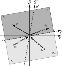
Figure 1: Space-time schematic diagram of superluminal space-time refraction. In the $S$ frame (bold), the optical perturbation is observed as moving along the $x$ axis (from left to right) with apparent velocity $u$ whereas, in the $S^{\prime}$ frame (dashed), the optical perturbation alters the refractive index of the medium simultaneously for all point of space at instant $t^{\prime}=0$. Both frames can be related using a standard Lorentz boost with $\beta=v_{\infty}/c=-c/u<1$.

Like Eq. (1), Eqs. (2) to (4) are also derived from the invariance of the phase of light between any two different inertial frames Mendoncabook and correspond to a double Doppler shift. For values $\theta_{i}\neq 0,\pi$, $\phi_{t}$ and $\phi_{r}$ are calculated as

$$\theta_{t} = \arctan\left[\sin\theta_{i}/\gamma^{2}\left(f+\sigma_{it}g_{t}\right)\right],$$ (5)

$$\theta_{r} = \arctan\left[\sin\theta_{i}/\gamma^{2}\left(f-\sigma_{ir}g_{r}\right)\right].$$ (6)

These expressions correspond to the generalized Fresnel formula for a moving superluminal partial mirror.

Using the continuity conditions for dielectric displacement and the magnetic induction fields Cirone ; Time Refraction at time $\mathbf{r}=t\mathbf{u}$, the annihilation and creation operators for these modes can be related as

$$a_{i}=Aa_{t}-Ba_{r}^{\dagger}\text{ and }a_{a}=Aa_{r}-Ba_{t}^{\dagger},$$ (7)

where $A=\left(1+\alpha^{2}\right)/2\alpha$, $B=\left(1-\alpha^{2}\right)/2\alpha$ and $\alpha=\left[n_{i}^{2}g_{i}h_{i}/n_{t}^{2}g_{t}h_{t}\right]^{1/2}$, satisfying $A^{2}-B^{2}=1$.

As demonstrated in Refs. Leonhardt ; Gilles , the two-mode squeezing transformation (7) implies that, after the optical perturbation has passed, an initial vacuum can be expressed in terms of the new eigenstates of the field as

$$\left|0\right\rangle_{i}\left|0\right\rangle_{a}=\sum{}_{n}C_{n}\left|n\right\rangle_{t}\left|n\right\rangle_{r},$$ (8)

with $C_{n}=\sqrt{1-\left|z\right|^{2}}z^{n}$ and $z=B/A$. Eq. (8) implies the emission of photon pairs moving along the different directions of $\mathbf{k}_{t}$ and $\mathbf{k}_{r}$, according to Eqs. (2) to (4). The mean photon number for wave vectors $\mathbf{k}_{t}$ and $\mathbf{k}_{r}$ is

$$\left\langle N_{t}\right\rangle=\left\langle N_{r}\right\rangle=\frac{|z|^{2}}{1-|z|^{2}}=\frac{\left[n_{i}^{2}h_{i}g_{i}-n_{t}^{2}h_{t}g_{t}\right]^{2}}{4n_{i}^{2}n_{t}^{2}h_{i}h_{t}g_{i}g_{t}}.$$ (9)

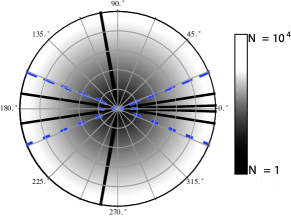
Figure 2: Emission spectrum: Angular distribution of the number of photons emitted by the optical boundary corresponding to a change of refractive index from $n_{i}=n_{a}=1.1$ to $n_{t}=n_{r}=1.5$ and for $\beta=0.9$ (dashed) and for $\beta=0.99$ (bold). Notice that the emission predominantly concentrated in a very small solid angle around the resonance angles. With $\beta=0.9$ there is only the resonance for $\beta n_{i}\cos\theta_{i}^{res}\rightarrow 1$, whereas with $\beta=0.99$, both resonances $\beta n_{i}\cos\theta_{i}^{res}\rightarrow 1$ and $\beta n_{r}\cos\theta_{r}^{res}\rightarrow 1$ exist.

According to Eq. (9) the number of photons emitted diverges for $z\rightarrow 1$. In the one-dimensional case studied in Guerreiro2005 this could only be achieved if a perfect matching between the velocity of the optical perturbation $u$ and $n_{i}$ such that $\beta n_{i}=cn_{i}/u\rightarrow 1$. However, in the three-dimensional case there is an extra degree of freedom corresponding to the angle between the wave vector and the direction of the apparent motion of the optical perturbation, and the condition $z\rightarrow 1$ can be achieved for both $\beta n_{i}\cos\theta_{i}^{res}\rightarrow 1$ and/or $\beta n_{r}\cos\theta_{r}^{res}\rightarrow 1$. Unlike the case of TR, the photon emission produced by a superluminal optical perturbation is not limited by the maximum variation of refractive index produced by optical perturbation. Instead, when the phase velocity of the waves $\phi_{i}$ and $\phi_{r}$ along $\mathbf{u}$ are identical to $\mathbf{u}$, corresponding respectively to $\beta n_{i}\cos\theta_{i}^{res}\rightarrow 1$ and/or $\beta n_{r}\cos\theta_{r}^{res}\rightarrow 1$, the optical perturbation and the waves $\phi_{i}$ and $\phi_{r}$ move together and can interact for longer times producing an arbitrarily large number of photons. This process can be described as a form of superluminal resonance. We identify three regimes: i) for $\beta n_{i}<1$ and $\beta n_{r}<1$ there are no resonances; ii) for either $\beta n_{i}>1$ or $\beta n_{r}>1$ there is only one pair of resonant emission angles; and iii) for both $\beta n_{i}>1$ or $\beta n_{r}>1$ two pairs of resonant light are emitted. An extra resonance also exists for $\beta=n$ in media such as plasmas, where the refractive index is lower than $1$ Guerreiro2005 , for simplicity we neglect this resonance herein. These resonances can be achieved for a wide range of experimental parameters and configurations. The angular distribution corresponding to Eq. (9) is represented in Figure 2 where we can clearly identify $\theta_{t}^{res}$ and $\theta_{r}^{res}$, calculated from $\theta_{i}^{res}$ using Eqs. (5) and (6) respectively. Notice that emission is mainly limited to a narrow solid angle, resulting in colimated beams.

Photonic entanglement generation. The field can be separated into two subsystems ($S$ and $S^{\prime}$) corresponding to the two distinct sets of photons emitted, i.e. $\phi_{r}$ and $\phi_{t}$. Depending on the initial state of the field, these two subsystems may become entangled after the optical perturbation. We discuss and compare the degree of entanglement between two situation: an initial vacuum and a thermal state (which is the experimental case).

According to Eq. (7), an initial vacuum state is changed into another pure state for which the entanglement entropy $E_{VN}(\rho_{SS^{\prime}})\equiv-\textrm{Tr}\left[\rho^{S}\ln\rho^{S}\right]$ (with $\rho^{S}=Tr_{S^{\prime}}\left[\rho_{SS^{\prime}}\right]$) is the canonical entanglement measure Shumacher , yielding $E_{VN}=\ln\left(1+\left\langle N_{t}\right\rangle\right)\left(1+\left\langle N_{t}\right\rangle\right)-\left\langle N_{t}\right\rangle\ln\left\langle N_{t}\right\rangle$. Notice that $E_{VN}$ is basically the Shannon entropy introduced by increasing a photon pair in the system. For $z\rightarrow 1$, the entanglement diverges as the system approaches the resonance condition and the maximal entanglement state is achieved, i.e.

$$\underset{z\rightarrow 1}{\lim}\left|0\right\rangle_{i}\left|0\right\rangle_{a}=\underset{N\rightarrow\infty}{\lim}\underset{n=0}{\overset{N}{\sum}}\frac{1}{\sqrt{N}}\left|n\right\rangle_{t}\left|n\right\rangle_{r}.$$ (10)

If the system is initially in a thermal state of both wave modes, $\phi_{i}$ and $\phi_{a}$, i.e. $\rho_{ia}(\bar{n})=\rho(\bar{n})\otimes\rho(\bar{n})$, with

$$\rho(\bar{n})=\frac{1}{1+\bar{n}}\sum_{n=0}^{\infty}\left(\frac{\bar{n}}{1+\bar{n}}\right)^{n}|n\rangle\langle n|,$$ (11)

where $\bar{n}$ is the thermal mean occupancy, then after the optical perturbation has passed, the state $\rho_{tr}(z)$ describing the $\phi_{t}$ and $\phi_{r}$ modes becomes $\rho_{tr}(z)=S(z)\rho_{ia}(\bar{n})S(z)^{\dagger}$, which is a squeezed thermal state Marian and for which $E_{VN}$ is not an adequate entanglement measure Plenio . However $\rho_{tr}$ is a Gaussian state, and its entanglement can be completely characterized using continuous variable methods (see Ferraro for a review), namely via the logarithmic negativity, $E_{N}(\rho)=\max\left[0,-\ln\mu\right]$, where $\mu$ is the smallest sympletic eigenvalue of the Gaussian state $\rho_{tr}$. The expression for $\mu$ (see Laurat for a derivation) is $\mu=\left(2\bar{n}+1\right)\exp\left(-2\text{arctanh}z\right)$. The latter defines a thermal occupancy $n_{c}$, above which all entanglement vanishes, yielding $2\bar{n}_{c}+1=\exp\left(2\text{arctanh}z\right).$ Close to resonance ($z\rightarrow 1$) the maximum allowable thermal occupancy diverges $\bar{n}_{c}\rightarrow\infty$; entailing that entanglement extraction from optical boundaries is very robust regarding temperature by choosing a sufficiently high $z$.

Discussion of efficiency. Now we consider an optical perturbation in a frame $S$ of the form, $n(x-ut)=n_{0}+\delta n\ f[K(x-ut)]$, where $K$ is a spatial scale describing the sharpness and duration of the optical perturbation and $f(x)=0$ for $x\leq 0$, $f(x)=x$ for $0<x\leq 1$ and $f(x)=1$ for $x>1$. In the $S^{\prime}$ frame, the creation and annihilation operators in the interaction picture satisfy Tito2005

$$\frac{d}{dt^{\prime}}a_{t}=\nu(t^{\prime})a_{r}^{\dagger},\ \frac{d}{dt^{\prime}}a_{r}^{\dagger}=\nu^{*}(t^{\prime})a_{t},$$ (12)

with $\nu(t^{\prime})=\nicefrac{{1}}{{2}}exp[2i\psi(t^{\prime})][\nicefrac{{d}}{{dt^{\prime}}}ln\ n^{\prime}]$, where $\psi(t^{\prime})$ is a phase. The total photon number $N=N_{t}+N_{r}$ satisfies

$$\frac{d^{2}}{dt^{\prime 2}}(N+2)=4\left|\nu(t^{\prime})\right|^{2}(N+2).$$ (13)

For a small variation of refractive index (i.e. $\delta n\ll n_{0}$), the total number of photons produced, the maximum and average rate of photon generation from initial thermal states are respectively

$$N_{total} \approx (N_{0}+2)\ \cosh(\eta\delta n)$$ (14)

$$R_{max} \equiv \frac{dN}{dt}\approx(N_{0}+2)\eta\delta nKu\ \sinh(\eta\delta n)$$ (15)

$$R_{mean} \approx (N_{0}+2)Ku\gamma^{-1}\ \cosh(\eta\delta n)$$ (16)

where $\eta\equiv\nicefrac{{d}}{{dn_{0}}}ln\ n_{0}^{\prime}$. For conditions close the resonances, $\eta\sim 1/(n_{0}\Delta)$, where $\Delta\equiv 1-\beta n\cos\theta$ is the detuning from the resonance conditions.

Conclusions. We presented an emission mechanism of entangled radiation using a sharp optical perturbation with an apparent superluminal velocity. The emission spectrum and the emissivity depend on the apparent velocity and the change of refractive index of the optical perturbation. These results extend those of reference Guerreiro2005 from a one-dimensional configuration to one that includes all complex plane-wave modes in a three-dimensional space and is valid for an arbitrary dispersive medium. For our particular configuration, the optimum direction of emission is defined by the resonances $\Delta_{i}\rightarrow 0$ and $\Delta_{r}\rightarrow 0$. The resonance angles $\theta_{t}^{res}$ and $\theta_{r}^{res}$ correspond to both the best radiance and to the optimally entangled photons. From a purely theoretical point of view, this process has considerable advantages over PDC as a source of entangled light, namely, since it is capable of delivering two well separable and highly entangled beams with large intensities. In our case the photons are entangled in momentum whereas in PDC the photons are entangled in polarization; however, these two types of entanglement can be interconverted Boschi . From a more experimental point of view, it is not easy to produce a sharp and sudden optical perturbation at scales inferior to the optical wavelengths to allow the large number of photon pairs necessary to make this process competitive with PDC. A conservative estimate based on parameters from present day experimental demonstrations of superluminal ionization frontsExperiments ; Kostin ; TeraHz Pulses ($\beta\approx 0.9995$, $K/c\approx 0.02fs$, assuming $\delta n/n_{0}\approx 1\%$) predicts photon yields in excess of $R_{max}\sim 10^{10}s^{-1}$ ($R_{mean}\sim 10^{9}s^{-1}$) for $\Delta\sim 0.01$. Moreover, a recent work has shown that this quantum mechanism of extracting photon pairs out of ZPF can be extended to optical perturbations with arbitrary shape as long as they have an apparent superluminal velocity Tito2005 . These results suggest the possibility of generating high intensity entangled photons via specific time-dependent optical perturbations, including dynamical Casimir effect.

A. G. acknowledges the support of the Casimir network of the European Science Foundation. A.F. acknowledges the support of FCT (Portugal) through grant PRAXIS no. SFRH/BD/18292/04.

References

- (1) C. H. Bennett, D. P. DiVincenzo, Nature (London), 404, 247 (2000).
- (2) D. Bouwmeester, et al., Nature (London), 390, 6660 (1997).
- (3) A. Ferreira, A. Guerreiro, and V. Vedral, Phys. Rev. Lett. 96, 060407 (2006).
- (4) S. Bose, et al., Phys. Rev. Lett. 87, 050401 (2001).
- (5) R. Ursin, et al., Nature Physics 3, 481 (2007).
- (6) R. Boyd, Nonlinear Optics, Academic Press (1992).
- (7) A. Valencia, et al., Phys. Rev. Lett., 88, 183601 (2002).
- (8) S. Tanzilli et al., Electron. Lett. 37, 26-28 (2001).
- (9) S.L. Braunstein, Quantum computation, tutorial. In: Quantum Computation: Where Do We Want to Go Tomorrow?, Wiley-VCH, Weinheim (1999).
- (10) E. Yablonovitch, Phys. Rev. Lett., 62, 1743 (1989).
- (11) L.O. Silva and J.T. Mendonça, IEEE Trans. Plasma Sci., 24, 2 (1996).
- (12) D.L. Fisher and T. Tajima, Phys. Rev. Lett., 71, 4338 (1993).
- (13) D.L. Lampe, E. Ott and J.H. Walker, Phys. Fluids., 10, 43 (1978).
- (14) K. B. Kuntz et al., Phys. Rev. A 79, 043802 (2009).
- (15) V. A. Kostin and N. V. Vedenskii, Opt. Lett. 35, 247 (2010).
- (16) J.T. Mendonça, A. Guerreiro and A.M. Martins, Phys. Rev. A, 62, 033805 (2000).
- (17) J.T. Mendonça, The Theory of Photon Acceleration., Institute of Physics Publishing Bristol (2000).
- (18) A. Guerreiro, Journal of Plasma Physics, 76, 833-843 (2010).
- (19) W.G. Unruh, Phys. Rev. D, 14, 870 (1976).
- (20) S.W. Hawking, Nature(Lond.), 248 30 (1974); ibidem, Commn. Math. Phys., 43 199 (1975).
- (21) V.V. Dodonov, A. B. Klimov, V. I. Man’ko, Phys. Lett. A, 149, 225 (1990); C. K. Law, Phys. Rev.A, 49, 433 (1994); V. V. Dodonov, Phys. Rev. Lett., 207, 126 (1995); M. Cirone, O. Méplan and C. Gignoux, Phys. Rev. Lett., 76, 408 (1996); R. Rgazewsky and Mostowski, Phys. Rev. A, 55, 62 (1997) and R. Schültzhold, G. Plunien, and G. Soff, Phys. Rev. A, 57, 2311 (1998).
- (22) A. Guerreiro, J.T. Mendonça and A.M. Martins, J. Opt. B: Quantum Semiclass. Opt., 7, S69 (2005).
- (23) M. Cirone, R. Rgazewsky, and J. Mostowsky, Phys. Rev. A, 55, 62 (1997).
- (24) U. Leonhardt, Phys. Rev. A, 49, 1231 (1994).
- (25) L. Gilles and P.L. Knight, J. Mod. Opt., 39, 1411 (1992).
- (26) C.H. Bennett, et al., Phys. Rev. A 53, 2046 (1996). C.H. Bennett, et al., Phys. Rev. Lett. 76, 722 (1996).
- (27) P. Marian, and T. A. Marian, Phys. Rev. A, 45, 4474 (1993).
- (28) M. B. Plenio, and S. Virmani, Quant. Inf. Comp. 7, 1 (2007).
- (29) A. Ferraro, S. Olivares, M. G. A. Paris, pre-print: quant-ph/0503237 (2005).
- (30) J. Laurat et. al., J. Opt. B, 7, S577 (2005).
- (31) J. T. Mendonça, and A. Guerreiro, Phys. Rev. A, 72, 063805 (2005).
- (32) D. Boschi, et. al., Phys. Rev. Lett., 80, 1121 (1998).
- (33) Klaas Wynne and Dino A. Jaroszynski, Optics Letters, 24, 25 (1999).