Radiative corrections in $K_{e4}$ decay

Yu.ย M.ย Bystritskiy bystr@theor.jinr.ru Joint Institute for Nuclear Research, 141980 Dubna,Russia โ€ƒโ€ƒ S.ย R.ย Gevorkyan111On leave of absence from Yerevan Physics Institute gevs@jinr.ru Joint Institute for Nuclear Research, 141980 Dubna,Russia โ€ƒโ€ƒ E.ย A.ย Kuraev kuraev@theor.jinr.ru Joint Institute for Nuclear Research, 141980 Dubna,Russia
Abstract

The final state interaction of pions in the decay $K^{\pm}\to\pi^{+}\pi^{-}e^{\pm}\nu$ allows to obtain the value of the isospin and angular momentum zero pion-pion scattering length $a_{0}^{0}$. To extract this quantity from experimental data the radiative corrections (RC) have to be taken into account. Basing on the lowest order results and the factorization hypothesis, we get the expressions for RC in the leading and next-to leading logarithmical approximation. It is shown that the decay width dependence on the lepton mass $m_{e}$ through the parameter $\sigma=\frac{\alpha}{2\pi}\left(\ln\frac{M^{2}}{m_{e}^{2}}-1\right)$ has a standard form of the Drell-Yan process and is proportional to the Sommerfeld-Sakharov factor. The numerical estimations are presented.

I Introduction

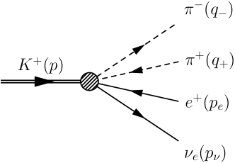
Kaons decay with two or three pions in the final state could give the unique information on the value of the s๐‘ s and $p$-wave pion-pion scattering lengths, whose values are predicted very precisely within Chiral Perturbation Theoryย Colangelo:2001df . The semi-leptonic decay known as $K_{e4}$ decay (for definiteness we will discuss the $K^{+}$ decay) (see Fig.ย 1):

Refer to caption
Figure 1: The semi-leptonic decay $K_{e4}$.
$\displaystyle K^{\pm}(p)\to\pi^{+}(q_{+})+\pi^{-}(q_{-})+e^{\pm}(p_{e})+\nu(p_{\nu})$ (1)

is very clean environment for the measurement of $\pi\pi$ scattering lengths, since the two pions are the only hadrons in the final state produced close to threshold.
Recently the high statistics measurement of $K_{e4}$ decay has been done by NA48/2 collaboration at the CERN SPSย Batley:2007zz .The high quality of this data allows one to extract the scattering length $a_{0}^{0}$ with accuracy comparable with theoretical predictions. From the other hand to obtain such high precision in scattering length determination from experimental data one would take into account all effects, which can have impact on the value of extracting quantity. One of such effects crucial in obtaining the scattering length value from experimental data is the correct accounting of radiative corrections in the decay (1). For RC calculations in decays like the Monte Carlo package PHOTOS has been developed ย Barberio:1990ms ; Barberio:1993qi and widely used in data processing. Unfortunately the PHOTOS does not take into account the electromagnetic interaction between charged pions in the final state effect, which is important near production thresholdย Gevorkyan:2006rh when the relative velocity in the pion pair becomes small. Moreover the Monte Carlo calculations are not transparent and require the special consideration of accuracy for any particular decay.
From the other hand a large improvement in accounting the RC in the decays with several hadrons in final state has been done recentlyย Isidori:2007zt ; Bissegger:2008ff . Later on we consider the full set of RC in the $K_{e4}$ decay and obtain the relevant expressions, which can be easily applied to actual calculations in the decay (1). Our expressions are in accordance with ones fromย Isidori:2007zt with two main difference. Despite the expressions in ย Isidori:2007zt our formulas are suitable for the case when one of the particle in the final state (lepton) differ from other (pions). Moreover we take into account also the radiation of hard photons, which leads to disappearance of cut in photon energy.
Before consideration of the proper RC let us shortly discuss the widely exploited approach ย Pais:1968zz to the process (1) without electromagnetic effects.The relevant matrix element can be expressed as

T=GF2โ€‹Vuโ€‹sโˆ—โ€‹(Vฮผโˆ’Aฮผ)โ€‹uยฏโ€‹(pฮฝ)โ€‹ฮณฮผโ€‹(1โˆ’ฮณ5)โ€‹vโ€‹(pe),๐‘‡subscript๐บ๐น2superscriptsubscript๐‘‰๐‘ข๐‘ superscript๐‘‰๐œ‡superscript๐ด๐œ‡ยฏ๐‘ขsubscript๐‘๐œˆsubscript๐›พ๐œ‡1subscript๐›พ5๐‘ฃsubscript๐‘๐‘’\displaystyle T=\frac{G_{F}}{\sqrt{2}}V_{us}^{*}\left(V^{\mu}-A^{\mu}\right)\bar{u}(p_{\nu})\gamma_{\mu}(1-\gamma_{5})v(p_{e}), (2)

where the axial and vector hadronic currents

$\displaystyle A^{\mu}$ $\displaystyle=$ $\displaystyle\frac{-i}{M}\left(\left(q_{+}+q_{-}\right)^{\mu}F+\left(q_{+}-q_{-}\right)^{\mu}G+\left(p_{e}+p_{\nu}\right)^{\mu}R\right);$
$\displaystyle V^{\mu}$ $\displaystyle=$ $\displaystyle\frac{-H}{M^{3}}\epsilon^{\mu\nu\rho\sigma}p_{\nu}\left(q_{+}+q_{-}\right)_{\rho}\left(q_{+}-q_{-}\right)_{\sigma},$ (4)

where $M$ is the K-meson mass. The contribution of the axial form factor R to the differential width is proportional to the square of electron mass and would be omitted. Confining by s and p waves and assuming the same p-wave phases for different form-factors:

F=Fsโ€‹eiโ€‹ฮดs+Fpโ€‹eiโ€‹ฮดp;G=Gpโ€‹eiโ€‹ฮดp;H=Hpโ€‹eiโ€‹ฮดp.formulae-sequence๐นsubscript๐น๐‘ superscript๐‘’๐‘–subscript๐›ฟ๐‘ subscript๐น๐‘superscript๐‘’๐‘–subscript๐›ฟ๐‘formulae-sequence๐บsubscript๐บ๐‘superscript๐‘’๐‘–subscript๐›ฟ๐‘๐ปsubscript๐ป๐‘superscript๐‘’๐‘–subscript๐›ฟ๐‘\displaystyle F=F_{s}e^{i\delta_{s}}+F_{p}e^{i\delta_{p}};\qquad G=G_{p}e^{i\delta_{p}};\qquad H=H_{p}e^{i\delta_{p}}. (5)

The aim of experimental investigation is to measure the quantities Fssubscript๐น๐‘ F_{s}, $F_{p}$, $G_{p}$, $H_{p}$ and the phases difference ฮด=ฮดsโˆ’ฮดp๐›ฟsubscript๐›ฟ๐‘ subscript๐›ฟ๐‘\delta=\delta_{s}-\delta_{p} as a function of dimensionless invariants sฯ€=(q++qโˆ’)2subscript๐‘ ๐œ‹superscriptsubscript๐‘žsubscript๐‘ž2s_{\pi}=(q_{+}+q_{-})^{2}, se=(pฮฝ+pe)2subscript๐‘ ๐‘’superscriptsubscript๐‘๐œˆsubscript๐‘๐‘’2s_{e}=(p_{\nu}+p_{e})^{2}.

Besides these variables there are three angles in use. Azimuthal angle $\phi$ between the plane containing the pions momenta in the kaon rest frame and the plane containing the electron and neutrino momenta; the polar angle $\theta_{\pi}$ between the positive charged pion and the dipion line and finally the polar angle $\theta_{e}$ between the electron momentum and the dilepton line.
The differential width has the form ย Pais:1968zz

dโ€‹ฮ“B=GF2โ€‹|Vuโ€‹s|22โ€‹(4โ€‹ฯ€)6โ€‹ฮ›1/2โ€‹(M2,sฯ€,se)โ€‹ฮฒโ€‹(1โˆ’me2se)2โ€‹Jโ€‹dโ€‹sฯ€โ€‹dโ€‹seโ€‹dโ€‹cosโกฮธฯ€โ€‹dโ€‹cosโกฮธeโ€‹dโ€‹ฯ•,๐‘‘subscriptฮ“๐ตsuperscriptsubscript๐บ๐น2superscriptsubscript๐‘‰๐‘ข๐‘ 22superscript4๐œ‹6superscriptฮ›12superscript๐‘€2subscript๐‘ ๐œ‹subscript๐‘ ๐‘’๐›ฝsuperscript1superscriptsubscript๐‘š๐‘’2subscript๐‘ ๐‘’2๐ฝ๐‘‘subscript๐‘ ๐œ‹๐‘‘subscript๐‘ ๐‘’๐‘‘subscript๐œƒ๐œ‹๐‘‘subscript๐œƒ๐‘’๐‘‘italic-ฯ•\displaystyle d\Gamma_{B}=\frac{G_{F}^{2}|V_{us}|^{2}}{2(4\pi)^{6}}\Lambda^{1/2}(M^{2},s_{\pi},s_{e})\beta(1-\frac{m_{e}^{2}}{s_{e}})^{2}Jds_{\pi}ds_{e}d\cos\theta_{\pi}d\cos\theta_{e}d\phi, (6)

where

$\displaystyle\Lambda(a,b,c)$ $\displaystyle=$ $\displaystyle a^{2}+b^{2}+c^{2}-2(ab+ac+bc)$

The structure J=Jโ€‹(sฯ€,se,ฮธฯ€,ฮธe,ฯ•)๐ฝ๐ฝsubscript๐‘ ๐œ‹subscript๐‘ ๐‘’subscript๐œƒ๐œ‹subscript๐œƒ๐‘’italic-ฯ•J=J(s_{\pi},s_{e},\theta_{\pi},\theta_{e},\phi) is the rather complicate function of four form-factorsย  Pais:1968zz , whereas ฮฒ=1โˆ’4โ€‹m2sฯ€๐›ฝ14superscript๐‘š2subscript๐‘ ๐œ‹\beta=\sqrt{1-\frac{4m^{2}}{s_{\pi}}} (m is the charged pion mass) is the relative velocity of pions in the kaon rest frame.

Calculation of radiative corrections , which is the motivation of our paper is performed in frames of unrenormalized theory. We introduce the fictitious mass of the photon $\lambda$ and momentum cut-off parameter $\Lambda$. The final result which takes into account emission of virtual and real photons would be free from infrared divergences connected with photon mass. Keeping in mind the renormalizability of the Standard Model the cut-off parameter $\Lambda$ at the final stage must be replaced by the W boson mass $M_{W}$.

Our paper is organized as follows. The explicit calculation of contributions of channels with virtual and real (soft and hard) photons in lowest order in fine structure constant are presented in the first two sections. The combined result in the lowest order of perturbation theory and its generalization to higher orders are given in two following sections.

Appendixย A contains the details of calculations of virtual and real photons emissions. Appendixย B contains the explicit forms of $K$, $K_{v}$, Kssubscript๐พ๐‘ K_{s} factors using in numerical calculations.

In Tableย 1 the result of a numerical estimations of a width and $K$ factors are given for several typical values of the kinematical invariants.

II Virtual photons emission

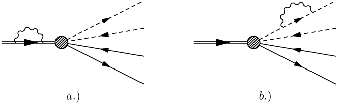
Let us at first shortly discuss the corrections arising from the virtual photon emission. An important ingredient in such consideration is the wave functions renormalization constants of electron and pseudoscalar mesons (see Fig.ย 2)

Refer to caption
Figure 2: Some typical graphs responsible for the renormalization of the wave functions.
$\displaystyle Z_{e}$ $\displaystyle=$ $\displaystyle\frac{\alpha}{2\pi}\left[-\frac{1}{2}L_{\Lambda}-\frac{3}{2}L_{e}+L_{\lambda}-\frac{9}{4}\right];\quad Z_{P}=\frac{\alpha}{2\pi}\left[L_{\Lambda}+L_{\lambda}-\frac{3}{4}\right]$
$\displaystyle L_{\Lambda}$ $\displaystyle=$ $\displaystyle\ln\frac{\Lambda^{2}}{m^{2}},\quad L_{e}=\ln\frac{m^{2}}{m_{e}^{2}},\quad L_{\lambda}=\ln\frac{m^{2}}{\lambda^{2}}.$ (7)

The relevant contribution to the differential widths (6) can be introduced by replacement

$\displaystyle J\to J\left(1+3Z_{p}+Z_{e}\right)$ (8)

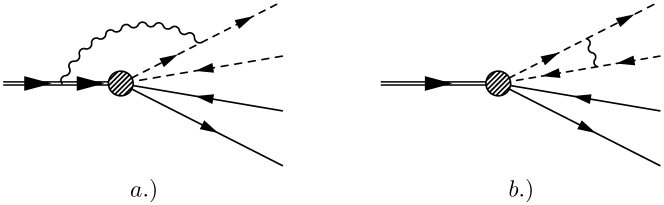
Neglecting structure emission (when photons are emitted from โ€hardโ€ hadronic or weak blocks) we have to consider six Feynman amplitudes with virtual photon attached to charged particles (see Fig.ย 3).

Refer to caption
Figure 3: Some graphs describing the virtual corrections to $K_{e4}$ decay.

Neglecting as well by the virtual photon momentum in the โ€hardโ€ block we obtain

$\displaystyle T^{v}$ $\displaystyle=$ $\displaystyle\frac{G_{F}V_{us}^{*}}{\sqrt{2}}(V^{\mu}-A^{\mu})\frac{\alpha}{4\pi}\int\frac{d^{4}k}{i\pi^{2}(k^{2}-\lambda^{2})}[\sum_{i=1}^{3}R_{i}\bar{u}(p_{\nu})\gamma_{\mu}(1-\gamma_{5})v(p_{e})$ (9)
$\displaystyle+$ $\displaystyle\sum_{i=1}^{3}Q_{i}^{\eta}\bar{u}(p_{\nu})\gamma_{\mu}(1-\gamma_{5})(-\hat{p}_{e}-\hat{k}+m_{e})\gamma_{\eta}v(p_{e})],$

with the following notations

$\displaystyle R_{1}$ $\displaystyle=$ $\displaystyle\frac{(-2q_{+}-k)_{\sigma}(-2p-k)^{\sigma}}{dd_{+}};\quad R_{2}=\frac{(2q_{-}+k)_{\sigma}(-2p-k)^{\sigma}}{dd_{-}};$
$\displaystyle R_{3}$ $\displaystyle=$ $\displaystyle\frac{(-2q_{+}+k)_{\sigma}(2q_{-}+k)^{\sigma}}{d_{-}d_{+}},$
$\displaystyle Q_{1}^{\eta}$ $\displaystyle=$ $\displaystyle\frac{(-2p-k)^{\eta}}{dd_{e}};\quad Q_{2}^{\eta}=\frac{(-2q_{+}k)^{\eta}}{d_{+}d_{e}};\quad Q_{3}^{\eta}=\frac{(2q_{-}-k)^{\eta}}{d_{-}d_{e}},$
$\displaystyle d$ $\displaystyle=$ $\displaystyle(p+k)^{2}-M^{2}+i0;\quad d_{+}=(-q_{+}+k)^{2}-m^{2}+i0;$
$\displaystyle d_{-}$ $\displaystyle=$ $\displaystyle(q_{-}-k)^{2}-m^{2}+i0;\quad d_{e}=(p_{e}+k)^{2}-m_{e}^{2}+i0.$ (10)

The contribution of virtual photon loops to the decay rate (6) is determined by the real part of the interference between the single loop and the Born amplitude (2). The standard integration of expression (9) leads to the following form of this interference

$\displaystyle J\left(1+3Z_{p}+Z_{e}+\frac{\alpha}{2\pi}\left[I_{1}+I_{2}+I_{4}+I_{3}+I_{5}+I_{6}\right]\right).$ (11)

The explicit form of the six integrals $I_{i}$ are given in Appendixย A. The assumption about smooth behavior of the structure Jโ€‹(sฯ€,sl,โ€ฆ)=J0๐ฝsubscript๐‘ ๐œ‹subscript๐‘ ๐‘™โ€ฆsubscript๐ฝ0J(s_{\pi},s_{l},...)=J_{0} allow us to write down the contribution from the emission of virtual photons as

$\displaystyle\frac{d\Gamma^{v}}{d\Gamma_{B}}$ $\displaystyle=$ $\displaystyle\frac{\alpha}{2\pi}\left[L_{\lambda}\left(4+\frac{1}{\beta_{-}}L_{-}-\frac{1}{\beta_{+}}L_{+}-2\rho-\frac{1+\beta^{2}}{\beta}L_{\beta}+2\ln{\frac{p_{e}q_{+}}{p_{e}q_{-}}}\right)\right.$ (12)
$\displaystyle+$ $\displaystyle\left.\pi^{2}\frac{1+\beta^{2}}{\beta}-2l\rho+4\rho+\frac{1}{2}\ln^{2}\frac{M^{2}}{m_{e}^{2}}+\frac{9}{4}L_{\Lambda}+K_{v}\right],$

Here $\rho=\ln\frac{2E_{e}}{m_{e}}$ is the โ€large logarithmโ€ ($E_{e}$, $E_{\pm}$ is the positron and pions energies in the kaon rest frame)

$\displaystyle L_{\pm}$ $\displaystyle=$ $\displaystyle\ln\frac{1+\beta_{\pm}}{1-\beta_{\pm}};\qquad\beta_{\pm}=\sqrt{1-\frac{m^{2}}{E_{\pm}^{2}}}$
$\displaystyle l$ $\displaystyle=$ $\displaystyle\ln\frac{M^{2}}{m^{2}};\qquad L_{\beta}=\ln\frac{1+\beta}{1-\beta};$ (13)

The explicit form of $K_{v}$ is cited in Appendixย B.

III Real photons emission

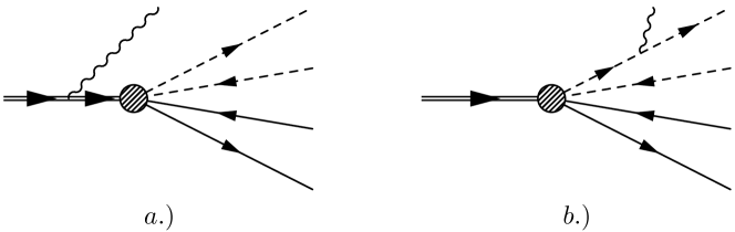
Let us now discuss the emission of real photons. The contribution of soft (in the kaon rest frame) photons is proportional to the decay width in Born approximation (see Fig.ย 4):

Refer to caption
Figure 4: Real photon emission corrections to $K_{e4}$ decay.
dโ€‹ฮ“sโ€‹oโ€‹fโ€‹tdโ€‹ฮ“B๐‘‘superscriptฮ“๐‘ ๐‘œ๐‘“๐‘ก๐‘‘subscriptฮ“๐ต\displaystyle\frac{d\Gamma^{soft}}{d\Gamma_{B}} $\displaystyle=$ $\displaystyle-\frac{\alpha}{4\pi^{2}}\int\frac{d^{3}k}{\omega}\left(\frac{p}{pk}+\frac{q_{-}}{q_{-}k}-\frac{q_{+}}{q_{+}k}-\frac{p_{e}}{p_{e}k}\right)^{2}_{\omega<\Delta\epsilon}$ (14)
$\displaystyle=$ ฮฑฯ€โ€‹ฮ”s,ฮ”โ€‹ฯตโ‰ชEe.much-less-than๐›ผ๐œ‹superscriptฮ”๐‘ ฮ”italic-ฯตsubscript๐ธ๐‘’\displaystyle\frac{\alpha}{\pi}\Delta^{s},\qquad\Delta\epsilon\ll E_{e}.

The standard calculations give

ฮ”ssuperscriptฮ”๐‘ \displaystyle\Delta^{s} $\displaystyle=$ $\displaystyle\ln\left(\frac{2\Delta\epsilon}{\lambda}\right)\left[-4-\frac{1}{\beta_{-}}L_{-}+\frac{1}{\beta_{+}}L_{+}+2\rho+\frac{1+\beta^{2}}{\beta}L_{\beta}-2\ln\frac{2p_{e}q_{+}}{2p_{e}q_{-}}\right]$ (15)
$\displaystyle+$ ฯโˆ’ฯ2+Ks.๐œŒsuperscript๐œŒ2subscript๐พ๐‘ \displaystyle\rho-\rho^{2}+K_{s}.

with expression for Kssubscript๐พ๐‘ K_{s} given in Appendix B.

It is easy to see that the sum of soft (eq. (14)) and virtual (eq.(12)) photons does not depend on the introduced above fictitious photon mass $\lambda$.

At small relative velocity of pions $\beta$ the term $\frac{\pi\alpha(1+\beta^{2})}{2\beta}$ in (12) corresponds to the well known Sommerfeld-Sakharov factor Sommerfeld:1939 ; Sakharov:1948yq

$\displaystyle S(\beta)=\frac{t}{1-exp(-t)}=1+\frac{1}{2}t+\frac{t^{2}}{12}+O(t^{3}),\qquad t=\frac{\pi\alpha(1+\beta^{2})}{\beta}.$ (16)

Due to the general statements of quantum mechanics this factor is factorized out from the differential width for the case of small $\beta$.
All terms containing the positron mass singularities (which contains the quantity $\rho$) can be written in form of the so called delta-part of positron non-singlet structure function $P_{\delta}$. As a result the contribution of soft and virtual photons can be written as

$\displaystyle 1$ $\displaystyle+$ dโ€‹ฮ“s+dโ€‹ฮ“vdโ€‹ฮ“B=[1+ฯƒโ€‹Pฮด]โ€‹(1+ฮฑฯ€โ€‹K)โ€‹Sโ€‹(ฮฒ)โ€‹SEโ€‹W,๐‘‘superscriptฮ“๐‘ ๐‘‘superscriptฮ“๐‘ฃ๐‘‘subscriptฮ“๐ตdelimited-[]1๐œŽsubscript๐‘ƒ๐›ฟ1๐›ผ๐œ‹๐พ๐‘†๐›ฝsubscript๐‘†๐ธ๐‘Š\displaystyle\frac{d\Gamma^{s}+d\Gamma^{v}}{d\Gamma_{B}}=\left[1+\sigma P_{\delta}\right]\left(1+\frac{\alpha}{\pi}K\right)~{}S(\beta)~{}S_{EW}, (17)
$\displaystyle P_{\delta}$ $\displaystyle=$ $\displaystyle 2\ln\Delta+\frac{3}{2},\quad\sigma=\frac{\alpha}{2\pi}(2\rho-1),\quad S_{EW}=1+\frac{9\alpha}{4\pi}\ln\frac{M_{W}^{2}}{m^{2}},$

where $\Delta=\frac{\Delta\epsilon}{E_{e}}\ll 1$.

The factor $S_{EW}$ is absorbed, when we use the renormalized quantities instead of bare ones

(GF2โ€‹Vuโ€‹s2)bโ€‹aโ€‹rโ€‹eโ€‹SEโ€‹W=GF2โ€‹Vuโ€‹s2.superscriptsuperscriptsubscript๐บ๐น2superscriptsubscript๐‘‰๐‘ข๐‘ 2๐‘๐‘Ž๐‘Ÿ๐‘’subscript๐‘†๐ธ๐‘Šsuperscriptsubscript๐บ๐น2superscriptsubscript๐‘‰๐‘ข๐‘ 2\displaystyle(G_{F}^{2}V_{us}^{2})^{bare}S_{EW}=G_{F}^{2}V_{us}^{2}. (18)

The expression for the quantity $K$ given in Appendixย B. The values of $K$, $K_{v}$, Kssubscript๐พ๐‘ K_{s} for several typical sets of the kinematic parameters are tabulated in Tableย 1.

It is convenient to separate the contribution from the emission of hard photons $\omega>\Delta\epsilon$ in two parts. First one takes into account the emission along the positron direction. Another one takes into account the remaining part of the angular phase volume.

The first one can be calculated using the so called โ€quasi-real electronsโ€ method Baier:1973ms :

dโ€‹ฮ“hโ€‹(sฯ€,sl,โ€ฆ)=โˆซslโ€‹(1+ฮ”)smโ€‹aโ€‹xdโ€‹ssโ€‹[Pฮธโ€‹(sls)โ€‹ฯƒ+ฮฑ2โ€‹ฯ€โ€‹(1โˆ’sls)]โ€‹๐‘‘ฮ“Bโ€‹(sฯ€,s,โ€ฆ),๐‘‘superscriptฮ“โ„Žsubscript๐‘ ๐œ‹subscript๐‘ ๐‘™โ€ฆsuperscriptsubscriptsubscript๐‘ ๐‘™1ฮ”subscript๐‘ ๐‘š๐‘Ž๐‘ฅ๐‘‘๐‘ ๐‘ delimited-[]subscript๐‘ƒ๐œƒsubscript๐‘ ๐‘™๐‘ ๐œŽ๐›ผ2๐œ‹1subscript๐‘ ๐‘™๐‘ differential-dsubscriptฮ“๐ตsubscript๐‘ ๐œ‹๐‘ โ€ฆ\displaystyle d\Gamma^{h}(s_{\pi},s_{l},...)=\int\limits_{s_{l}(1+\Delta)}^{s_{max}}\frac{ds}{s}\left[P_{\theta}(\frac{s_{l}}{s})\sigma+\frac{\alpha}{2\pi}(1-\frac{s_{l}}{s})\right]d\Gamma_{B}(s_{\pi},s,...), (19)

with smโ€‹aโ€‹x=(pโˆ’q+โˆ’qโˆ’)2=M2+sฯ€โˆ’2โ€‹Mโ€‹(E++Eโˆ’)subscript๐‘ ๐‘š๐‘Ž๐‘ฅsuperscript๐‘subscript๐‘žsubscript๐‘ž2superscript๐‘€2subscript๐‘ ๐œ‹2๐‘€subscript๐ธsubscript๐ธs_{max}=(p-q_{+}-q_{-})^{2}=M^{2}+s_{\pi}-2M(E_{+}+E_{-})

$\displaystyle P_{\theta}(z)=\frac{1+z^{2}}{1-z}.$ (20)

As for the contributions which is not enhanced by the โ€large logarithmโ€ factor their contribution can be estimated in the soft photon emission approximation. It can be obtained from the quantity ฮ”ssuperscriptฮ”๐‘ \Delta^{s} putting $\Delta\epsilon=\omega_{0}=M-2m$. Soft photons approximation turns out to be rather realistic. The typical error compared with the exact calculation in the same order of perturbation theory looks as

$\displaystyle 1+O\left(\left(\frac{\omega}{M}\right)^{2}\right),\quad\omega<\omega_{max}=M-2m,\quad\left(\frac{\omega}{M}\right)^{2}\sim 0.1.$ (21)

Combining the Born approximation and the lowest order results obtained above we get the following expression for decay width

dโ€‹ฮ“โ€‹(sฯ€,sl,โ€ฆ)=โˆซslsmโ€‹aโ€‹xdโ€‹ssโ€‹[ฮดโ€‹(1โˆ’sls)โ€‹Pฮด+ฯƒโ€‹Pโ€‹(sls)+ฮฑฯ€โ€‹Kโ€‹(sls)]โ€‹๐‘‘ฮ“Bโ€‹(sฯ€,s,โ€ฆ),๐‘‘ฮ“subscript๐‘ ๐œ‹subscript๐‘ ๐‘™โ€ฆsuperscriptsubscriptsubscript๐‘ ๐‘™subscript๐‘ ๐‘š๐‘Ž๐‘ฅ๐‘‘๐‘ ๐‘ delimited-[]๐›ฟ1subscript๐‘ ๐‘™๐‘ subscript๐‘ƒ๐›ฟ๐œŽ๐‘ƒsubscript๐‘ ๐‘™๐‘ ๐›ผ๐œ‹๐พsubscript๐‘ ๐‘™๐‘ differential-dsubscriptฮ“๐ตsubscript๐‘ ๐œ‹๐‘ โ€ฆ\displaystyle d\Gamma(s_{\pi},s_{l},...)=\int\limits_{s_{l}}^{s_{max}}\frac{ds}{s}\left[\delta(1-\frac{s_{l}}{s})P_{\delta}+\sigma P(\frac{s_{l}}{s})+\frac{\alpha}{\pi}K(\frac{s_{l}}{s})\right]d\Gamma_{B}(s_{\pi},s,...), (22)

with

$\displaystyle P(x)=\left(\frac{1+x^{2}}{1-x}\right)_{+}=\lim_{\Delta\to 0}\left[\theta(1-x-\Delta)P_{\theta}+\delta(1-x)P_{\delta}(x)\right],$ (23)

and the quantities $P_{\Delta},P_{\theta}(x)$ given above. The generalized function $P(x)$ is the kernel of the evolution equation of partonic operators of twist two Kuraev:1985hb .

IV Generalization to higher orders

The obtained result for the decay width with the radiative corrections in the lowest order of perturbation theory (PT) taken into account, permits the generalization to higher orders of PT in the so called leading logarithmic approximation (LLA).

Moreover the terms of order $\sigma^{n}\alpha$ (next to leading approximation (NLO)) as well can be taken into account if the explicit form of a $K$-factor is known.

In such a way we obtain

dโ€‹ฮ“โ€‹(sฯ€,sl,โ€ฆ)=โˆซslsmโ€‹aโ€‹xdโ€‹ssโ€‹๐‘‘ฮ“Bโ€‹(sฯ€,s,โ€ฆ)โ€‹Dโ€‹(sls,ฯƒ)โ€‹(1+ฮฑฯ€โ€‹Kโ€‹(sls)),๐‘‘ฮ“subscript๐‘ ๐œ‹subscript๐‘ ๐‘™โ€ฆsuperscriptsubscriptsubscript๐‘ ๐‘™subscript๐‘ ๐‘š๐‘Ž๐‘ฅ๐‘‘๐‘ ๐‘ differential-dsubscriptฮ“๐ตsubscript๐‘ ๐œ‹๐‘ โ€ฆ๐ทsubscript๐‘ ๐‘™๐‘ ๐œŽ1๐›ผ๐œ‹๐พsubscript๐‘ ๐‘™๐‘ \displaystyle d\Gamma(s_{\pi},s_{l},...)=\int\limits_{s_{l}}^{s_{max}}\frac{ds}{s}d\Gamma_{B}(s_{\pi},s,...)D\left(\frac{s_{l}}{s},\sigma\right)\left(1+\frac{\alpha}{\pi}K\left(\frac{s_{l}}{s}\right)\right), (24)

with the structure function $D^{NS}(x,\sigma)=D(x,\sigma)$ has a form:

$\displaystyle D^{NS}(x,\sigma)$ $\displaystyle=$ $\displaystyle\delta(1-x)+\sigma P(x)+\frac{1}{2!}\sigma^{2}P^{(2)}(x)+...$
$\displaystyle P^{(n)}(x)$ $\displaystyle=$ $\displaystyle\int\limits_{x}^{1}\frac{dy}{y}P\left(y\right)P^{(n-1)}\left(\frac{x}{y}\right),\quad P^{(1)}(x)=P(x),$
$\displaystyle\sigma$ $\displaystyle=$ $\displaystyle\frac{\alpha}{2\pi}(2\rho-1),\quad n=2,3,...$ (25)

In applications it is convenient to use the smoothed form of $D(x,\sigma)$

$\displaystyle D(x,\sigma)=2\sigma(1-x)^{2\sigma-1}\left(1+\frac{3}{2}\sigma\right)-(1+x)\sigma+O(\sigma^{2}).$ (26)

The quantity $K$ accumulates all terms which are nonsingular in the limit of zero positron mass. It includes the contribution from emission of virtual and real photons. Its explicit form is given in Appendixย B. In the Tableย 1 we cite the values of $K$ for several typical values of the kinematic parameters.

Using the above expressions we can written the final expression for decay width in the form (we imply the smooth behavior of the Born width)

dโ€‹ฮ“dโ€‹ฮ“B=Sโ€‹(ฮฒ)โ€‹(1+ฮฑฯ€โ€‹K)โ€‹Fโ€‹(slsmโ€‹aโ€‹x,ฯƒ)๐‘‘ฮ“๐‘‘subscriptฮ“๐ต๐‘†๐›ฝ1๐›ผ๐œ‹๐พ๐นsubscript๐‘ ๐‘™subscript๐‘ ๐‘š๐‘Ž๐‘ฅ๐œŽ\displaystyle\frac{d\Gamma}{d\Gamma_{B}}=S(\beta)\left(1+\frac{\alpha}{\pi}K\right)F\left(\frac{s_{l}}{s_{max}},\sigma\right) (27)
$\displaystyle F(z,\sigma)=2\sigma\left(1+\frac{3}{2}\sigma\right)\int_{z}^{1}\frac{dx}{x}(1-x)^{2\sigma-1}-\sigma\left(\ln\frac{1}{z}+1-z\right).$ (28)

In experimental set-up when the averaging on the positron spectrum is accepted all the dependence on positron mass disappears in correspondence with Kinoshita-Lee-Nauenberg theorem

โˆซ0smโ€‹aโ€‹xdโ€‹ฮ“dโ€‹slโ€‹๐‘‘sl=Sโ€‹(ฮฒ)โ€‹โˆซ0smโ€‹aโ€‹xdโ€‹ฮ“Bdโ€‹slโ€‹(1+ฮฑฯ€โ€‹K)โ€‹๐‘‘sl.superscriptsubscript0subscript๐‘ ๐‘š๐‘Ž๐‘ฅ๐‘‘ฮ“๐‘‘subscript๐‘ ๐‘™differential-dsubscript๐‘ ๐‘™๐‘†๐›ฝsuperscriptsubscript0subscript๐‘ ๐‘š๐‘Ž๐‘ฅ๐‘‘subscriptฮ“๐ต๐‘‘subscript๐‘ ๐‘™1๐›ผ๐œ‹๐พdifferential-dsubscript๐‘ ๐‘™\displaystyle\int\limits_{0}^{s_{max}}\frac{d\Gamma}{ds_{l}}ds_{l}=S(\beta)\int\limits_{0}^{s_{max}}\frac{d\Gamma_{B}}{ds_{l}}\left(1+\frac{\alpha}{\pi}K\right)ds_{l}. (29)

The vanishing of dependence on positron mass in our case it due to the structure function normalization $\int_{0}^{1}D(x,\sigma)dx=1$.

The values of $K$-factors for different kinematic variables (see eqs. (39), (40), (41)) and the function $F(z,\sigma)$ (eq. (28)) for $\sigma=0.0156$ are presented in the Tableย 1 and on Fig.ย 5.

V Summary

We calculated the full set of radiation correction for the decay width of the $K_{e4}$ in the lowest order in fine structure constant. It is shown that the sum of contribution from virtual and soft real photons emission is independent of fictitious mass of photon $\lambda$. The ratio of the decay width to its Born approximation is proportional to Sommerfeld-Sakharov factor, leading to the enhancement of the radiation correction at small relative velocity of two charged pions in the final state. The radiation of hard photons has been taken in account. It has been shown that all terms including large logarithms (including parameter $\rho=\ln{\frac{2E_{e}}{m_{e}}}$) are factorized in separate factor which depends on the correlation between electron and pions energies. The utilized approach allow us to generalize the low order results to higher orders of perturbative theory not only in leading logarithmic approximation (LLA), but even in next to leading order approximation (NLA). The numerical calculations are done for K factor and fragmentation function Fโ€‹(slsmโ€‹aโ€‹x,ฯƒ)๐นsubscript๐‘ ๐‘™subscript๐‘ ๐‘š๐‘Ž๐‘ฅ๐œŽF(\frac{s_{l}}{s_{max}},\sigma).

Acknowledgements.
We are grateful to Alexander Tarasov for interest in this problem and useful discussions. The work of two of us (Yu.ย M.ย B. and E.ย A.ย K.) was partially supported by INTAS grant 05-1000008-8528.
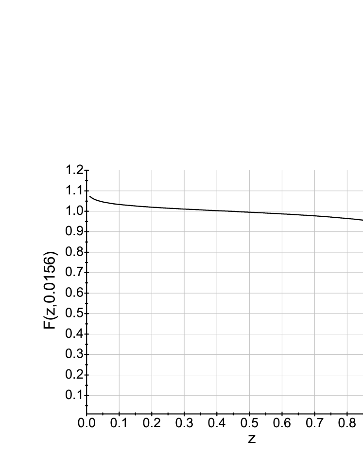
Refer to caption
Figure 5: The dependence of fragmentation function on lepton energy (see (28)).
$x_{+}$ $x_{-}$ $x_{e}$ $y_{+}$ $y_{-}$ Kssubscript๐พ๐‘ K_{s} $K_{v}$ K
0.3 0.3 0.4 2 2 -1.99 -6.12 -5.72
0.3 0.3 0.4 3 1 0.83 -8.06 -5.79
0.3 0.3 0.3 1 2 -3.42 -4.45 -5.01
0.3 0.3 0.3 1.5 1.5 -1.71 -5.85 -5.30
0.3 0.3 0.2 0.9 0.9 -1.37 -5.86 -4.82
0.3 0.3 0.1 0.25 0.25 -0.91 -6.79 -4.14
0.3 0.4 0.2 2 1 -0.14 -7.54 -5.81
0.3 0.4 0.2 1.5 1.5 -1.59 -6.14 -5.26
0.4 0.4 0.1 1 2 -3.01 -6.31 -4.68
Table 1: The values of the $K$-factors at some typical values of kinematical variables (see eqs. (39), (40), (41)).

Appendix A Integrals

A.1 Virtual photons emission

Applying the Feynman denominators joining procedure and performing the loop momentum integration, we obtain the explicit expressions for the integrals $I_{i}$ in interference term (11) through the Feynman parameter

$\displaystyle I_{1}$ $\displaystyle=$ $\displaystyle 1+L_{\Lambda}-l+\int_{0}^{1}\frac{dx}{X_{1}}\left(2x+2(1-x)x_{+}-2x_{+}(\ln X_{1}+l+L_{\lambda})\right);$
$\displaystyle I_{2}$ $\displaystyle=$ $\displaystyle-I_{1}(x_{+}\to x_{-});\quad X_{1}=x^{2}+(1-x)^{2}\eta^{2}+2x(1-x)x_{+};$
$\displaystyle I_{3}$ $\displaystyle=$ $\displaystyle 1+L_{\Lambda}-l+\int\limits_{0}^{1}\frac{dx}{X_{3}}\left(2x+4(1-x)x_{e}-2x_{e}(\ln(\frac{X_{3}}{\eta^{2}})+L_{\lambda})\right),$
$\displaystyle X_{3}$ $\displaystyle=$ $\displaystyle x^{2}+(1-x)^{2}\frac{m_{e}^{2}}{M^{2}}+2x(1-x)x_{e};$
$\displaystyle I_{4}$ $\displaystyle=$ $\displaystyle 1+L_{\Lambda}+\frac{2}{1-\beta^{2}}\int\limits_{0}^{1}\frac{dx}{X_{4}}\left((1+\beta^{2})(\ln{X_{4}}+L_{\lambda})-\beta^{2}\right),$
$\displaystyle X_{4}$ $\displaystyle=$ $\displaystyle 1-\frac{4x(1-x)}{1-\beta^{2}};$
$\displaystyle I_{5}$ $\displaystyle=$ $\displaystyle 1+L_{\Lambda}+\int\limits_{0}^{1}\frac{dx}{X_{5}}\left(2x-2(1-x)y_{-}-y_{-}(\ln{X_{5}}+L_{\lambda})\right);$
$\displaystyle I_{6}$ $\displaystyle=$ $\displaystyle-I_{5}(q_{-}\to q_{+});\quad X_{5}=x^{2}+\frac{m_{e}^{2}}{m^{2}}(1-x)^{2}-y_{-}x(1-x)].$ (30)

Here we use the following notations:

$\displaystyle x_{\pm}$ $\displaystyle=$ $\displaystyle\frac{E_{\pm}}{M};\quad x_{e}=\frac{E_{e}}{M};\quad y_{+}=\frac{2q_{+}p_{e}}{m^{2}};\quad y_{-}=\frac{2q_{-}p_{e}}{m^{2}};$
$\displaystyle y_{q}$ $\displaystyle=$ $\displaystyle\frac{2q_{+}q_{-}}{m^{2}}=\frac{2(1+\beta^{2})}{1-\beta^{2}};\quad\eta=\frac{m}{M}.$ (31)

Using the neutrino shell mass condition ($p_{\nu}^{2}=0$) one obtains the following relation between these variables

$\displaystyle y_{q}=\frac{2}{\eta^{2}}(-\frac{1}{2}+x_{+}+x_{-}+x_{e})-2-y_{+}-y_{-}.$ (32)

The integration in (30) can be done with the result (we systematically omit the terms which do not contribute in the limit of zero positron mass)

$\displaystyle\frac{2pq_{+}}{M^{2}}\int_{0}^{1}{\frac{dx}{X_{1}}}$ $\displaystyle=$ $\displaystyle\frac{1}{\beta_{+}}L_{+};\quad\frac{2q_{-}q_{+}}{m^{2}}Re\int_{0}^{1}\frac{dx}{X_{4}}=-\frac{1+\beta^{2}}{\beta}L_{\beta};$
$\displaystyle\frac{2pp_{e}}{M^{2}}\int_{0}^{1}\frac{dx}{X_{3}}$ $\displaystyle=$ $\displaystyle 2\rho;\quad\frac{2p_{e}q_{-}}{m^{2}}Re\int_{0}^{1}\frac{dx}{X_{5}}=-\ln{y_{-}}-\ln{\frac{m}{m_{e}}}$
$\displaystyle\frac{2pp_{e}}{M^{2}}\int_{0}^{1}\frac{dx}{X_{3}}\ln X_{3}$ $\displaystyle=$ $\displaystyle\ln^{2}2x_{e}-\frac{1}{2}\ln^{2}\frac{M^{2}}{m_{e}^{2}}-2Li_{2}(1-\frac{1}{2x_{e}});$
$\displaystyle\frac{2q_{+}q_{-}}{m^{2}}Re\int_{0}^{1}\frac{dx}{X_{4}}\ln X_{4}$ $\displaystyle=$ $\displaystyle\frac{1+\beta^{2}}{\beta}\left(\pi^{2}+Li_{2}(-\frac{2\beta}{1-\beta})-Li_{2}(\frac{2\beta}{1+\beta})\right);$
$\displaystyle\frac{2p_{e}q_{-}}{m^{2}}Re\int_{0}^{1}\frac{dx}{X_{5}}\ln X_{5}$ $\displaystyle=$ $\displaystyle\pi^{2}-\ln^{2}y_{-}+\frac{1}{2}\ln^{2}\frac{m^{2}}{m_{e}^{2}}+2Li_{2}(1+\frac{1}{y_{-}}).$ (33)

A.2 Soft photons emission

The integration in (14) has been done using the relation

$\displaystyle\int_{0}^{\Delta\epsilon}\frac{k^{2}dk}{\omega^{3}}f\left(\frac{k}{\omega}\right)=\int_{0}^{\Delta\epsilon}\frac{dk}{\omega}f\left(\frac{k}{\omega}\right)-\int_{0}^{\Delta\epsilon}\frac{\lambda^{2}dk}{\omega^{3}}f\left(\frac{k}{\omega}\right)$ (34)

where $\omega=\sqrt{k^{2}+\lambda^{2}}$ with $\lambda$ the โ€photon massโ€. Introducing the variable $t=k/\omega$ one obtains

$\displaystyle\int_{0}^{\Delta\epsilon}\frac{k^{2}dk}{\omega^{3}}f\left(\frac{k}{\omega}\right)=f\left(1\right)\ln\left(\frac{2\Delta\epsilon}{\lambda}\right)+\int_{0}^{1}\frac{dt}{1-t^{2}}\left[t^{2}f\left(t\right)-f\left(1\right)\right].$ (35)

Angular integration has been done using the relation ย Kuraev:1980

$\displaystyle d\Omega=2\frac{dc_{1}dc_{2}}{\sqrt{1-c_{1}^{2}-c_{2}^{2}-c^{2}+2cc_{1}c_{2}}},$ (36)

Here $c_{1,2}$ are the cosine of the angles between 3-vectors $\vec{k}$ and $\vec{p}_{1,2}$ and $c$ is the cosine of the angle between the 3-vectors $\vec{p}_{1}$ and $\vec{p}_{2}$.
Using these relations one gets

$\displaystyle\left.\frac{1}{4\pi}\int\frac{d^{3}k}{\omega}\frac{p_{1}p_{2}}{(p_{1}k)(p_{2}k)}\right|_{\omega<\Delta\epsilon}$ $\displaystyle=$ $\displaystyle f_{12}(1)\ln(\frac{2\Delta\epsilon}{\lambda})+\int_{0}^{1}\frac{dt}{1-t^{2}}(t^{2}f_{12}(t)-f_{12}(1));$
$\displaystyle f_{12}(t)=\frac{1}{4\pi}\int\frac{d\Omega}{(1-b_{1}c_{1})(1-b_{2}c_{2})}\frac{(p_{1}p_{2})}{\epsilon_{1}\epsilon_{2}}$ $\displaystyle=$ $\displaystyle\frac{1-\beta_{1}\beta_{2}c}{\sqrt{d}}\ln\frac{1-b_{1}b_{2}c+\sqrt{d}}{\sqrt{(1-b_{1}^{2})(1-b_{2}^{2})}};$
$\displaystyle\beta_{1}\beta_{2}c=1-\frac{(p_{1}p_{2})}{\epsilon_{1}\epsilon_{2}};\quad b_{1,2}=t\beta_{1,2},\quad\beta_{i}$ $\displaystyle=$ $\displaystyle\sqrt{1-m_{i}^{2}/\epsilon_{i}^{2}};$
$\displaystyle d$ $\displaystyle=$ $\displaystyle(1-b_{1}b_{2}c)^{2}-(1-b_{1}^{2})(1-b_{2}^{2}).$ (37)

Substituting in this expression the relevant momenta we obtain the terms determining the contribution of soft photons emission in considered decay rate

$\displaystyle\left.\frac{1}{4\pi}\int\frac{d^{3}k}{\omega}\frac{q_{+}q_{-}}{(q_{+}k)(q_{-}k)}\right|_{\omega<\Delta\epsilon}$ $\displaystyle=$ $\displaystyle\frac{1+\beta^{2}}{2\beta}\ln(\frac{2\Delta\epsilon}{\lambda})+I_{q};I_{q}=\int_{0}^{1}\frac{dt}{1-t^{2}}(t^{2}f_{q}(t)-f_{q}(1));$
$\displaystyle\left.\frac{1}{4\pi}\int\frac{d^{3}k}{\omega}\frac{p_{e}q_{+}}{(p_{e}k)(q_{+}k)}\right|_{\omega<\Delta\epsilon}$ $\displaystyle=$ $\displaystyle\ln\frac{2p_{e}q_{+}}{m_{e}m}\ln(\frac{2\Delta\epsilon}{\lambda})-\frac{1}{4}(2\rho^{2}+\frac{\pi^{2}}{6})+I_{e+};$
$\displaystyle I_{e_{+}}$ $\displaystyle=$ $\displaystyle(1-\beta_{+}c_{+})\int_{0}^{1}\frac{dt}{1-t^{2}}[-\frac{1}{2}(\frac{t^{2}}{\sqrt{d_{e}(t)}}-\frac{1}{1-\beta_{+}c_{+}})\ln(1-t^{2})$
$\displaystyle+$ $\displaystyle\frac{t^{2}}{\sqrt{d_{e}(t)}}\ln\frac{1-t^{2}\beta_{+}c_{+}+\sqrt{d_{e}(t)}}{\sqrt{1-t^{2}\beta_{+}^{2}}}-\frac{1}{1-\beta_{+}c_{+}}\ln\frac{2(1-\beta_{+}c_{+})}{\sqrt{1-\beta_{+}^{2}}}];$
$\displaystyle I_{q}$ $\displaystyle=$ $\displaystyle\int_{0}^{1}\frac{dt}{1-t^{2}}(t^{2}f_{q}(t)-f_{q}(1));\quad f_{q}(t)=\frac{1-\beta_{+}\beta_{-}c}{\sqrt{d_{q}(t)}}\ln\frac{1-t^{2}\beta_{+}\beta_{-}c+\sqrt{d_{q}(t)}}{\sqrt{(1-t^{2}\beta_{+}^{2})(1-t^{2}\beta_{-}^{2})}};$
$\displaystyle d_{q}(t)$ $\displaystyle=$ $\displaystyle(1-\beta_{+}\beta_{-}t^{2}c)^{2}-(1-\beta_{+}^{2}t^{2})(1-\beta_{-}^{2}t^{2});\quad\beta_{+}\beta_{-}c=1-\frac{\eta^{2}y_{q}}{2x_{+}x_{-}};$
$\displaystyle d_{e}(t)$ $\displaystyle=$ $\displaystyle(1-t^{2}\beta_{+}c_{+})^{2}-(1-t^{2})(1-t^{2}\beta_{+}^{2});\quad\beta_{+}c_{+}=1-\frac{\eta^{2}y_{+}}{2x_{+}x_{e}}.$ (38)

Finally we cited the result of integration of the squares of terms in (14)

$\displaystyle\left.\frac{1}{4\pi}\int\frac{d^{3}k}{\omega}(\frac{p}{pk})^{2}\right|_{\omega<\Delta\epsilon}$ $\displaystyle=$ $\displaystyle\ln\frac{2\Delta\epsilon}{\lambda}-1;$
$\displaystyle\left.\frac{1}{4\pi}\int\frac{d^{3}k}{\omega}(\frac{q_{\pm}}{q_{\pm}k})^{2}\right|_{\omega<\Delta\epsilon}$ $\displaystyle=$ $\displaystyle\ln\frac{2\Delta\epsilon}{\lambda}-\frac{1}{\beta_{\pm}}L_{\pm};$
$\displaystyle\left.\frac{1}{4\pi}\int\frac{d^{3}k}{\omega}\frac{pq_{\pm}}{(pk)(q_{\pm}k)}\right|_{\omega<\Delta\epsilon}$ $\displaystyle=$ $\displaystyle\frac{1}{2\beta_{\pm}}\left[\ln\frac{2\Delta\epsilon}{\lambda}L_{\pm}+\frac{1}{2}Li_{2}(-\frac{2\beta_{\pm}}{1-\beta_{\pm}})-\frac{1}{2}Li_{2}(\frac{2\beta_{\pm}}{1+\beta_{\pm}})\right].$

Appendix B K-factors

As an independent set of kinematical variables we choose the five independent variables: $x_{+}$, $x_{-}$, $x_{e}$, $y_{+}$, $y_{-}$.

The sum of terms independent from lepton mass is written in the form of so called $K$-factor has the form

$\displaystyle K$ $\displaystyle=$ Kv+Ks+ln2โก(2โ€‹xe)โˆ’32โ€‹lnโกฮท+lnโก(1โˆ’2โ€‹ฮท)+lnโก2+12โ€‹lnโก(2โ€‹xe)+34subscript๐พ๐‘ฃsubscript๐พ๐‘ superscript22subscript๐‘ฅ๐‘’32๐œ‚12๐œ‚2122subscript๐‘ฅ๐‘’34\displaystyle K_{v}+K_{s}+\ln^{2}(2x_{e})-\frac{3}{2}\ln\eta+\ln(1-2\eta)+\ln 2+\frac{1}{2}\ln(2x_{e})+\frac{3}{4} (39)
$\displaystyle+$ $\displaystyle\ln\left(\frac{1-2\eta}{\eta}\right)\left[-4-\frac{1}{\beta_{-}}L_{-}+\frac{1}{\beta_{+}}L_{+}+\frac{1+\beta^{2}}{\beta}L_{\beta}+2\ln\frac{y_{-}}{y_{+}}\right];$
$\displaystyle K_{v}$ $\displaystyle=$ $\displaystyle\int_{0}^{1}\frac{dx}{X_{1}}\left[-x_{+}\ln X_{1}+x+2(1-x)x_{+}+2x_{+}\ln\eta\right]+\frac{1}{2}\ln^{2}y_{+}-Li_{2}\left(1+\frac{1}{y_{+}}\right)$ (40)
$\displaystyle-$ $\displaystyle\frac{5}{2}\ln y_{+}-\left[x_{+}\to x_{-},y_{+}\to y_{-}\right]-\frac{5}{4}+\ln\eta-\frac{1}{2}\ln^{2}(2x_{e})+Li_{2}\left(1-\frac{1}{2x_{e}}\right)-\ln(2x_{e})$
$\displaystyle+$ $\displaystyle\frac{\beta}{2}L_{\beta}+\frac{1+\beta^{2}}{2\beta}\left[Li_{2}\left(-\frac{2\beta}{1-\beta}\right)-Li_{2}\left(\frac{2\beta}{1+\beta}\right)\right];$
Kssubscript๐พ๐‘ \displaystyle K_{s} $\displaystyle=$ $\displaystyle\frac{1}{2\beta_{+}}\left[Li_{2}\left(-\frac{2\beta_{+}}{1-\beta_{+}}\right)-Li_{2}\left(\frac{2\beta_{+}}{1+\beta_{+}}\right)\right]$ (41)
$\displaystyle-$ $\displaystyle 2I_{e+}-\left[x_{+}\to x_{-}\right]+1-\frac{\pi^{2}}{6}+\frac{1}{2\beta_{-}}L_{-}+\frac{1}{2\beta_{+}}L_{+}+2I_{q}.$

References

  • (1) G.ย Colangelo, J.ย Gasser, and H.ย Leutwyler, Nucl. Phys. B603, 125 (2001), hep-ph/0103088.
  • (2) NA48/2, J.ย R. Batley etย al., Eur. Phys. J. C54, 411 (2008).
  • (3) E.ย Barberio, B.ย van Eijk, and Z.ย Was, Comput. Phys. Commun. 66, 115 (1991).
  • (4) E.ย Barberio and Z.ย Was, Comput. Phys. Commun. 79, 291 (1994).
  • (5) S.ย R. Gevorkyan, A.ย V. Tarasov, and O.ย O. Voskresenskaya, Phys. Lett. B649, 159 (2007), hep-ph/0612129.
  • (6) G.ย Isidori, Eur. Phys. J. C53, 567 (2008), 0709.2439.
  • (7) M.ย Bissegger, A.ย Fuhrer, J.ย Gasser, B.ย Kubis, and A.ย Rusetsky, Nucl. Phys. B806, 178 (2009), 0807.0515.
  • (8) A.ย Pais and S.ย B. Treiman, Phys. Rev. 168, 1858 (1968).
  • (9) A.ย Sommerfeld, โ€Atombau und Spectrallinienโ€, 2 (1939), Vieweg, Braunschweig.
  • (10) A.ย D. Sakharov, Zh. Eksp. Teor. Fiz. 18, 631 (1948).
  • (11) V.ย N. Baier, V.ย S. Fadin, and V.ย A. Khoze, Nucl. Phys. B65, 381 (1973).
  • (12) E.ย A. Kuraev and V.ย S. Fadin, Sov. J. Nucl. Phys. 41, 466 (1985).
  • (13) E.ย A. Kuraev, Preprint INP, Novosibirsk 80-155, 1 (1980).