Fully 3D Multiple Beam Dynamics Processes Simulation for the Tevatron

Abstract

We present validation and results from a simulation of the Fermilab Tevatron including multiple beam dynamics effects. The essential features of the simulation include a fully 3D strong-strong beam-beam particle-in-cell Poisson solver, interactions among multiple bunches and both head-on and long-range beam-beam collisions, coupled linear optics and helical trajectory consistent with beam orbit measurements, chromaticity and resistive wall impedance. We validate individual physical processes against measured data where possible, and analytic calculations elsewhere. Finally, we present simulations of the effects of increasing beam intensity with single and multiple bunches, and study the combined effect of long-range beam-beam interactions and transverse impedance. The results of the simulations were successfully used in Tevatron operations to support a change of chromaticity during the transition to collider mode optics, leading to a factor of two decrease in proton losses, and thus improved reliability of collider operations.

I Motivation

The Fermilab Tevatron Tevatron is a $p$-$\bar{p}$ collider operating at a center-of-mass energy of $1.96\,\rm{TeV}$ and peak luminosity reaching $3.53\times 10^{32}\,\rm{cm}^{-2}\,~{}\rm{s}^{-1}$. The colliding beams consist of 36 bunches moving in a common vacuum pipe. For high-energy physics operations, the beams collide head-on at two interation points (IPs) occupied by particle detectors. In the intervening arcs the beams are separated by means of electrostatic separators; long-range (also referred to as parasitic) collisions occur at 136 other locations. Effects arising from both head-on and long-range beam-beam interactions impose serious limitations on machine performance, hence constant efforts are being exerted to better understand the beam dynamics. Due to the extreme complexity of the problem a numerical simulation appears to be one of the most reliable ways to study the performance of the system.

Studies of beam-beam interactions in the Tevatron Run II mainly concentrated on the incoherent effects, which were the major source of particle losses and emittance growth. This approach was justified by the fact that the available antiproton intensity was a factor of 10 to 5 less than the proton intensity with approximately equal transverse emittances. Several simulation codes were developed and used for the optimization of the collider performance lifetrac ; BBSim .

With the commissioning of electron cooling in the Recycler, the number of antiprotons available to the collider substantionally increased. During the 2007 and 2008 runs the initial proton and antiproton intensities differed by only a factor of 3. Moreover, the electron cooling produces much smaller transverse emittance of the antiproton beam ($\simeq 4\pi\,\textrm{mm}\,\textrm{mrad}$ 95% normalized vs. $\simeq 20\pi\,\textrm{mm}\,\textrm{mrad}$ for protons), leading to the head-on beam-beam tune shifts of the two beams being essentially equal. The maximum attained total beam-beam parameter for protons and antiprotons is 0.028.

Under these circumstances coherent beam-beam effects may become an issue. A number of theoretical works exist predicting the loss of stability of coherent dipole oscillations when the ratio of beam-beam parameters is greater than $\simeq 0.6$ due to the suppression of Landau dampingAlexahin . Also, the combined effect of the machine impedance and beam-beam interactions in extended length bunches couples longitudinal motion to transverse degrees of freedom and may produce a dipole or quadrupole mode instability combinedbb .

Understanding the interplay between all these effects requires a comprehensive simulation. This paper presents a macroparticle simulation that includes the main features essential for studying the coherent motion of bunches in a collider: a self-consistent 3D Poisson solver for beam-beam force computation, multiple bunch tracking with the complete account of sequence and location of long-range and head-on collision points, and a machine model including our measurement based understanding of the coupled linear optics, chromaticity, and impedance.

In Sections II–V we describe the simulation subcomponents and their validation against observed effects and analytic calculations. Section VI shows results from simulation runs which present studies of increasing the beam intensity. Finally, in Section VII we study the coherent stability limits for the case of combined resistive wall impedance and long-range beam-beam interactions.

II BeamBeam3d code

The Poisson solver in the BeamBeam3d code is described in Ref. Qiang1 . Two beams are simulated with macroparticles generated with a random distribution in phase space. The accelerator ring is conceptually divided into arcs with potential interaction points at the ends of the arcs. The optics of each arc is modeled with a $6\times 6$ linear map that transforms the phase space $\{x,x^{\prime},y,y^{\prime},z,\delta\}$ coordinates of each macroparticle from one end of the arc to the other. There is significant coupling between the horizontal and vertical transverse coordinates in the Tevatron. For our Tevatron simulations, the maps were calculated using coupled lattice functions Optim1 obtained by fitting a model ColOptics of beam element configuration to beam position measurements. The longitudinal portion of the map produces synchrotron motion among the longitudinal coordinates with the frequency of the synchrotron tune. Chromaticity results in an additional momentum-dependent phase advance $\delta\mu_{x(y)}=\mu_{0}C_{x(y)}\Delta p/p$ where $C_{x(y)}$ is the normalized chromaticity for $x$ (or $y$) and $\mu_{0}$ is the design phase advance for the arc. This is a generalization of the definition of chromaticity to apply to an arc, and reduces to the normalized chromaticity $({\Delta\nu}/\nu)/({\Delta p/p})$ when the arc encompasses the whole ring. The additional phase advance is applied to each particle in the decoupled coordinate basis so that symplecticity is preserved.

The Tevatron includes electrostatic separators to generate a helical trajectory for the oppositely charged beams. The mean beam offset at the IP is included in the Poisson field solver calculation.

Different particle bunches are individually tracked through the accelerator. They interact with each other with the pattern and locations that they would have in the actual collider.

The impedance model applies a momentum kick to the particles generated by the dipole component of resistive wall wakefields Chao1 . Each beam bunch is divided longitudinally into slices containing approximately equal numbers of particles. As each bunch is transported through an arc, particles in slice $i$ receive a transverse kick from the wake field induced by the dipole moment of the particles in forward slice $j$:

$${\Delta\vec{p}_{\perp}\over p}={2\over{\pi b^{3}}}\sqrt{{4\pi\epsilon_{0}c}\over\sigma}\,\,{N_{j}r_{0}\,{<\!\vec{r}_{j}\!>}\over{\beta\gamma}}{L\over\sqrt{z_{ij}}}$$ (1)

The length of the arc is $L$, $N_{j}$ is the number of particles in slice $j$, $r_{0}$ is the classical electromagnetic radius of the beam particle $e^{2}/4\pi\epsilon_{0}m_{0}c^{2}$, $z_{ij}$ is the longitudinal distance between the particle in slice $i$ that suffers the wakefield kick and slice $j$ that induces the wake. $\vec{r}_{j}$ is the mean transverse position of particles in slice $j$, $b$ is the pipe radius, $c$ is the speed of light, $\sigma$ is the conductivity of the beam pipe and $\beta\gamma$ are Lorentz factors of the beam. Quantities with units are specified in the MKSA system.

III Synchrobetatron comparisons

We will assess the validity of the beam-beam calculation by comparing simulated synchrobetatron mode tunes with a measurement performed at the VEPP-2M $500\,{\rm MeV}$ $e^{+}e^{-}$ collider and described in Ref. Nesterenko . These modes are an unambiguous marker of beam-beam interactions and provide a sensitive tool for evaluating calculational models. These modes arise in a colliding beam accelerator where the longitudinal bunch length and the transverse beta function are of comparable size. Particles at different $z$ positions within a bunch are coupled through the electromagnetic interaction with the opposing beam leading to the development of coherent synchrobetatron modes. The tune shifts for different modes have a characteristic evolution with beam-beam parameter $\xi=Nr_{0}/4\pi\gamma\epsilon$, in which $N$ is the number of particles, $r_{0}$ is the classical electromagnetic radius of the beam particle, and $\epsilon$ is the unnormalized one-sigma beam emittance.

There are two coherent transverse modes in the case of simple beam-beam collisions between equal intensity beams without synchrotron motion: the $\sigma$ mode where the two beams oscillate with the same phase, and the $\pi$ mode where the two beams oscillate with opposite phases piwinski . Without synchrotron motion, the $\sigma$ mode mode has the same tune as unperturbed betatron motion while the $\pi$ mode frequency is offset by $K\xi$, where the parameter $K$ is approximately equal to and greater than 1 and depends on the transverse shape of the beams yokoya . The presence of synchrotron motion introduces a more complicated spectrum of modes whose spectroscopy is outlined in Fig. 1 in Ref. Nesterenko .

We simulated the VEPP-2M collider using Courant-Snyder uncoupled maps. The horizontal emittance in the VEPP-2M beam is much larger than the vertical emittance. The bunch length ($4\,{\rm cm}$) is comparable to $\beta^{*}_{y}=6\,{\rm cm}$ so we expect to see synchrobetatron modes. In order to excite synchrobetatron modes, we set an initial $y$ offset of one beam sigma approximately matching the experimental conditions.

Longitudinal effects of the beam-beam interaction were simulated by dividing the bunch into six slices. At the interaction point, bunches drift through each other. Particles in overlapping slices are subjected to a transverse beam-beam kick calculated by solving the 2D Poisson equation for the electric field with the charge density from particles in the overlapping beam slice.

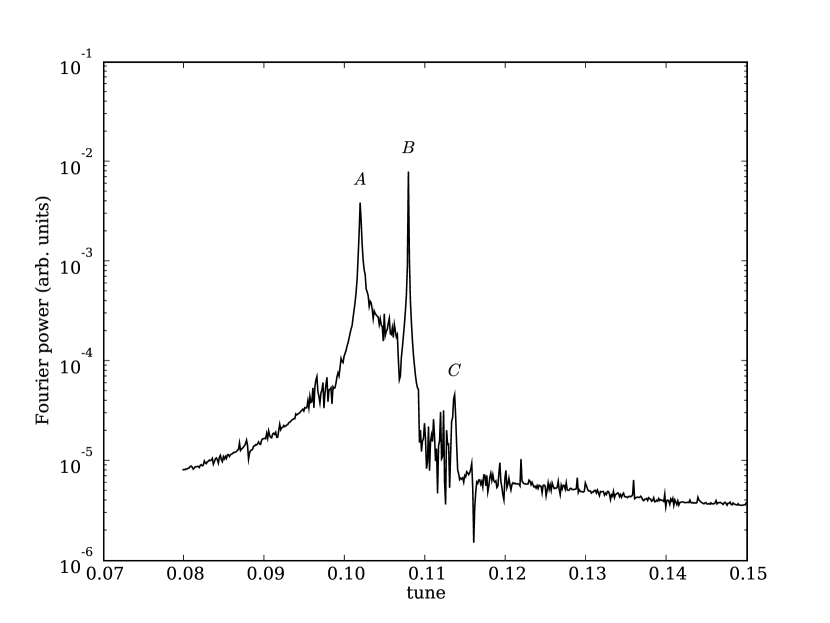
Figure 1: Simulated mode spectra in the VEPP-2M collider with $\xi=.008$ showing synchrobetatron modes. The line indicated by A is the base tune, B is the first synchrobetatron mode, C is the beam-beam $\pi$ mode.

Simulation runs with a range of beam intensities corresponding to beam-beam parameters of up to 0.015 were performed, in effect mimicking the experimental procedure described in Ref. Nesterenko . For each simulation run, mode peaks were extracted from the Fourier transform of the mean bunch vertical position. An example of the spectrum from such a run is shown in Fig. 1 with three mode peaks indicated. In Fig. 2, we plot the mode peaks from the BeamBeam3d simulation as a function of $\xi$ as red diamonds overlaid on experimental data from Ref. Nesterenko and a model using linearized coupled modes referred to as the matrix model described in that reference and Ref. Perevedentsev_Valishev ; Danilov_Perevedentsev . As can be seen, there is good agreement between the observation and simulation giving us confidence in the beam-beam calculation.

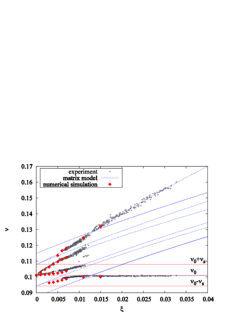
Figure 2: The diamonds show simulated synchrobetatron modes as a function of beam-beam parameter $\xi$ (diamonds) and of observed modes (points).

IV Impedance tests

Wakefields or, equivalently, impedance in an accelerator with a conducting vacuum pipe gives rise to well known instabilities. Our aim in this section is to demonstrate that the wakefield model in BeamBeam3d quantitatively reproduced these theoretically and experimentally well understood phenomena. The strong head-tail instability examined by Chao Chao1 arises in extended length bunches in the presence of wakefields. For any particular accelerator optical and geometric parameters, there is an an intensity threshold above which the beam becomes unstable.

The resistive wall impedance model applies an additional impulse kick in addition to the application of the map derived from beam optics. The tune spectrum is computed from the Fourier transform of the beam bunch positions sampled at the end of each arc. In order for the calculation to be a good approximation of the wakefield effect, the impedance kick should be much smaller than the $x^{\prime}$ or $y^{\prime}$ change due to regular beam transport so we divide the ring into multiple arcs. which brings up the question is how many is sufficient. The difference in calculated impedance tune shift for a 12 arc division of the ring or a 24 arc division is only $2\times 10^{-4}$, which is less than 3% of the synchrotron tune (0.007 in this study), the relevant scale in these simulations. We perform the calculation with 12 arcs for calculational efficiency.

In the absence of impedance, we would expect to see the tune spectrum peak at 20.574, the betatron tune of the lattice. With a pipe radius of $3\,{\rm cm}$ and a bunch length of $20\,{\rm cm}$, resistive wall impedance produces the spectrum shown in Fig. 3 for a bunch of $4\times 10^{12}$ protons at $150\,{\rm GeV}$. In this simulation, the base tune $\nu_{\beta}$ is $20.574$ and the synchrotron tune is $0.007$. Three mode peaks are clearly evident corresponding to synchrobetatron modes with frequencies $\nu_{\beta}-\nu_{s}$ shifted up by the wakefield (point $A$), $\nu_{\beta}$ shifted down (point $B$), and $\nu_{\beta}+\nu_{s}$ shifted upward (point $C$) as would be expected in Ref. chao_strong_headtail .

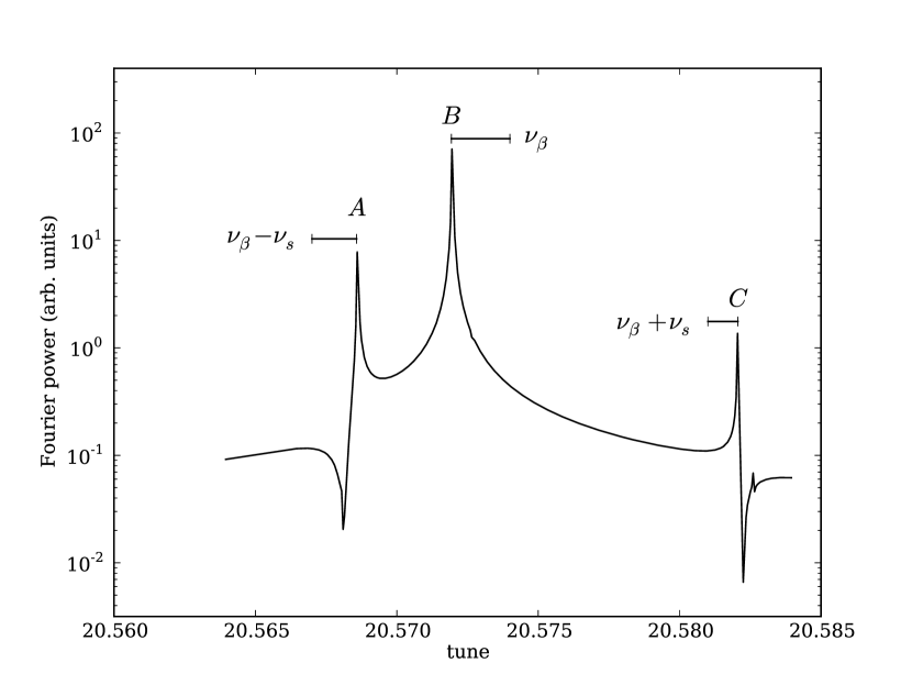
Figure 3: Simulated spectrum of a two slice bunch in the presence of wakefields and synchrotron motion showing three synchrobetatron modes $A$, $B$, and $C$ induced by wakefields.

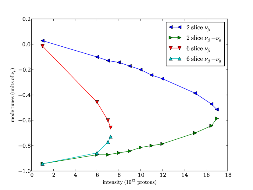
Figure 4: Evolution of the base tune and lower synchrobetatron mode frequencies as a function of beam intensity showing the two modes approaching a common frequency due to impedance. The $y$ scale is in units of the synchrotron tune. The simulations are shown for a two slice aond six slice wakefield calculation.

In Fig. 4, we show the evolution of the two modes as a function of beam intensity. With the tune and beam environment parameters of this simulation, Chao’s two particle model predicts instability development at intensities of about $9\times 10^{12}$ particles, which is close to where the upper and lower modes meet. We show two sets of curves for two slice and six slice wakefield calculations. The difference between the two slice and six slice simulations is accounted for by the effective slice separation, $\hat{z}$, that enters Eq. 1. With two slices, the effective $\hat{z}$ is larger than than the six slice effective $\hat{z}$, resulting in a smaller $W_{0}$. With the smaller wake strength, a larger number of protons is necessary to drive the two modes together as is seen in Fig. 4.

When the instability occurs, the maximum excursion of the bunch dipole moment grows exponentially as the beam executes turns through the accelerator. The growth rate can be determined by reading the slope of a graph of the absolute value of bunch mean position as a function of turn number plotted on a log scale. The growth rate per turn of dipole motion at the threshold of strong head-tail instability has a parabolic dependence on beam intensity. The wakefield calculation reproduces this feature, as shown in Fig. 5. The growth rate is slowly increasing up to the instability threshold at $5.42\times 10^{12}$, after which it has the explicitly quadratic dependence on beam intensity ($I$) of $\textrm{growth rate}=-0.100+0.0304I-0.00207I^{2}$.

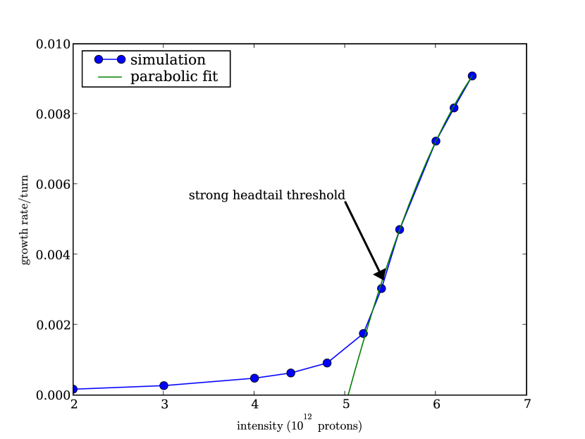
Figure 5: The growth rate of dipole motion in the simulated accelerator with impedance as a function of beam intensity as the strong head-tail threshold is reached superimposed with a parabolic fit.

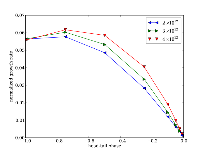
Figure 6: The normalized growth rate of dipole motion in the simulated accelerator with impedance and chromaticity as a function of head-tail phase $\chi$ at three beam intensities demonstrating their linear relationship close to $0$ and the near-universal relationship for head-tail phase between $-1$ and $0$.

Chromaticity interacts with impedance to cause a different head-tail instability. We simulated a range of beam intensities and chromaticity values. The two particle model and the more general Vlasov equation calculation Chao1 indicate that the growth rate scales by the head-tail phase $\chi=2\pi C\nu_{\beta}{\hat{z}}/c\eta$, where $\eta$ is the slip factor of the machine and $\hat{z}$ is roughly the bunch length. The head-tail phase gives the size of betatron phase variation due to chromatic effects over the length of the bunch.

Some discussion of the meaning of the slip factor in the context of a simulation is necessary. In a real accelerator, the slip factor has an unambiguous meaning: $\eta=(\alpha_{C}-1/\gamma^{2})$. The momentum compaction parameter $\alpha_{c}$ is determined by the lattice and $\gamma$ is the Lorentz factor. We simulate longitudinal motion by applying maps to the particle coordinates $z$ and $\delta$ in discrete steps. The simulation parameters specifying longitudinal transport are the longitudinal beta function $\beta_{z}$ and synchrotron tune $\nu_{s}$. Note that these parameters do not make reference to path length travelled by a particle. However, path length enters into the impedance calculation because wake forces are proportional to path length. In addition, analytic calculations of the effect of wake forces depend on the evolution of the longitudinal particle position which in turn depend explicitly on the slip factor. For our comparisons with analytic results to be meaningful, we need to use a slip factor that is consistent with the longitudinal maps and the path lengths that enter the wake force calculations. The relationship between the slip factor $\eta$ and the simulation parameters is $\beta_{z}=\eta L_{\bigcirc}/2\pi\nu_{s}$, where $L_{\bigcirc}$ is the length of the accelerator and $\beta_{z}=\sigma_{z}/\sigma_{\delta}$ is the longitudinal beta functionChao2 ; Syphers which may be derived by identifying corresponding terms in the solution to the differential equations of longitudinal motion and a one term linear map.

When the growth rate is normalized by $Nr_{0}W_{0}/2\pi\beta\gamma\nu_{\beta}$, which includes the beam intensity and geometric factors, we expect a universal dependence of normalized growth rate versus head-tail phase that begins linearly with head-tail phaseChao3 and peaks around -1.

Fig. 6 shows the simulated growth rate at three intensities with a range of chromaticites from $-.001$ to $-0.5$ to get head-tail phases in the $0$ to $-1$ range. The normalized curves are nearly identical and peak close to head-tail phase of unity. The deviation from a universal curve is again due to differences between the idealized model and detailed simulation.

V Bunch-by-bunch emittance growth at the Tevatron

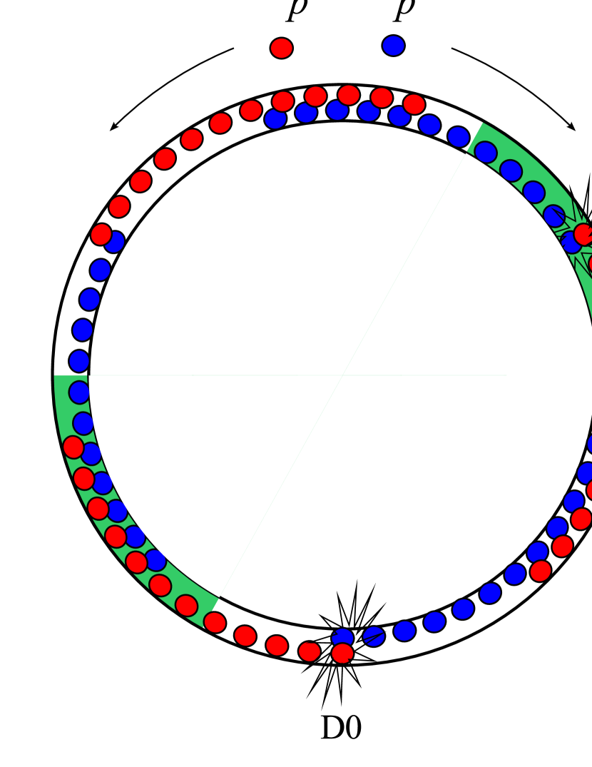
Figure 7: Schematic of the position of proton and antiproton bunches in the Tevatron with 36 proton and 36 antiproton bunches. The diagram shows the positions at a time when the lead bunch of the trains are at the head-on collision location. Head-on collisions occur at location B0 and D0. The green shading indicates the part of the ring where beam-beam collisions may occur in the simulations with six-on-six bunches.

Understanding the effect of unwanted long-range collisions among multiple beam bunches in the design and operation of hadron colliders has received attention from other authors pieloni ; lifetrac which underscores the importance for this kind of simulation. A schematic of the fill pattern of proton and antiproton bunches in the Tevatron is shown in Fig. 7. There are three trains of twelve bunches for each species. A train occupies approximately $81.5^{\circ}$ separated by a gap of about $38.5^{\circ}$. The bunch train and gap are replicated three times to fill the ring. Bunches collide head-on at the B0 and D0 interaction points but undergo long range (electromagnetic) beam-beam interactions at 136 other locations around the ring.

Running the simulation with all 136 long-range IPs turns out to be very slow so we only calculated beam-beam forces at the two main IPs and and the long-range IPs immediately upstream and downstream of them. The transverse beta functions at the long-range collision locations are much larger than the bunch length, so the beam-beam calculation at those locations can be performed using only the 2D solver.

One interesting consequence of the fill pattern and the helical trajectory is that any one of the 12 bunches in a train experiences collisions with the 36 bunches in the other beam at different locations around the ring, and in different transverse positions. This results in a different tune and emittance growth for each bunch of a train, but with the three-fold symmetry for the three trains. In the simulation, emittance growth arises from the effects of impedance acting on bunches that have been perturbed by beam-beam forces. The phenomenon of bunch dependent emittance growth is observed experimentallyshiltsev_beambeam .

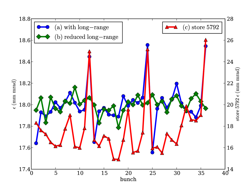
Figure 8: The simulated and measured emittance of each Tevatron proton bunch after running with 36 proton and 36 antiproton bunches. Curves (a) and (b) which show the emittance after 50000 simulated turns are read with the left vertical axis. Curve (a) results from a simulation with the nominal beam spacing at the long-range IPs. Curve (b) results from a simulation with the hypothetical condition where the beam separation at the long-range IPs is 100 times normal, suppressing the effect of those long-range IPs. Curve (c) is the measured emittance of bunches after 15 minutes of a particular store (#5792) of bunches in the Tevatron, and is read with the right vertical axis.

The beam-beam simulation with 36-on-36 bunches shows similar effects. We ran a simulation of 36 proton on 36 antiproton bunches for 50000 turns with the nominal helical orbit. The proton bunches had $8.8\times 10^{11}$ particles (roughly four times the usual to enhance the effect) and the proton emittance was the typical $20\pi\,\textrm{mm}\,\textrm{mrad}$. The antiproton bunch intensity and emittance were both half the corresponding proton bunch parameter. The initial emittance for each proton bunch was the same so changes during the simulation reflect the beam-beam effect.

Curve (a) in Figure 8 shows the emittance for each of the 36 proton bunches in a 36-on-36 simulation after 50000 turns of simulation. The three-fold symmetry is evident. The end bunches of the train (bunch 1, 13, 25) are clearly different from the interior bunches. For comparison, curve (c) shows the measured emittance taken during accelerator operations. The observed bunch emittance variation is similar to the simulation results. Another beam-beam simulation with the beam separation at the closest head-on IP expanded 100 times its nominal value resulted in curve (b) of Figure 8 showing a much reduced bunch-to-bunch variation. We conclude that the beam-beam effect at the long-range IPs is the origin of the bunch variation observed in the running machine and that our simulation of the beam helix is correct.

VI Tevatron applications

VI.1 Single bunch features

We looked at the tune spectrum with increasing intensity for equal intensity $p$ and $\bar{p}$ beams containing one bunch each. As the intensity increases, the beam-beam parameter $\xi$ increases. Fig. 9 shows the spectrum of the sum and difference of the two beam centroids for $\xi=0.01,0.02,0.04$, corresponding to beam bunches containing $2.2\times 10^{11}$, $4.4\times 10^{11}$ and $8.8\times 10^{11}$ protons. The abscissa is shifted so the base tune is at 0 and normalized in units of the beam-beam parameter at a beam intensity of $2.2\times 10^{11}$. The coherent $\sigma$ and $\pi$ mode peaks are expected to be present in the spectra of the sum and difference signals of the two beam centroids. The coherent $\sigma$ modes are evident at 0, while the coherent $\pi$ modes should slightly greater than 1, 2, and 4 respectively. Increasing intensity also causes larger induced wake fields which broaden the mode peaks, especially the $\pi$ mode, as shown in Fig. 9.

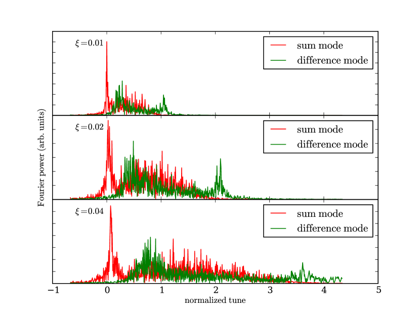
Figure 9: Dipole mode spectra of the sum and difference offsets of two beam centroids at three beam intensities corresponding to beam-beam parameter values for each beam of 0.01, 0.02 and 0.04. The vertical scale is in arbitrary units.

The 4D emittances at higher intensities show significant growth over 20000 turns as shown in Fig. 10. The kurtosis excess of the two beams remains slightly positive for the nominal intensity, but shows a slow increase at higher intensities indicating the the beam core is being concentrated as shown in Fig. 11. Concentration of the bunch core while emittance is growing indicates the development of filamentation and halo.

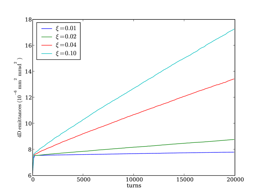
Figure 10: The evolution of 4D emittances for beam-beam parameters of 0.01, 0.02, and 0.04 which correspond to intensities of (a) $2.2\times 10^{11}$, (b) $4.4\times 10^{11}$, (c) $8.8\times 10^{11}$, and (d) $1.1\times 10^{12}$ protons per bunch.

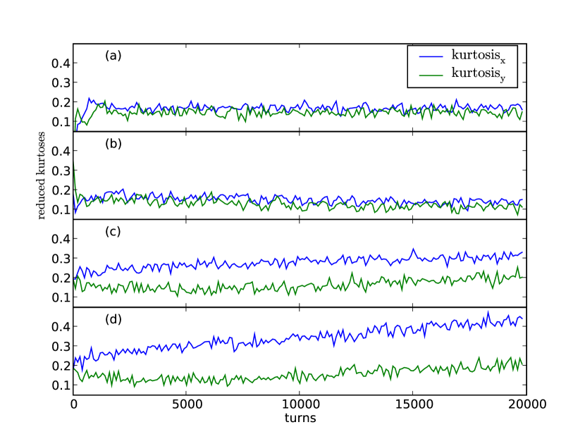
Figure 11: The evolution of (reduced) kurtosis of the particle distribution for intensities of (a) $2.2\times 10^{11}$, (b) $4.4\times 10^{11}$, (c) $8.8\times 10^{11}$, and (d) $1.1\times 10^{12}$ protons per bunch.

VI.2 Simulation of bunch length, synchrotron motion and beam-beam interactions

Synchrotron motion in extended length bunches modifies the effects of the beam-beam interaction by shifting and suppressing the coherent modes. The plots in Fig. 12 show simulated spectra for sum and difference signals of the beam centroid offsets for one-on-one bunch collisions in a ring with Tevatron-like optics, with both short and long bunches, at three different synchrotron tunes. The sum signal will contain the $\sigma$ mode while the difference signal will contain the $\pi$ mode. In this Tevatron simulation, the beam strength is set so that the beam-beam parameter is 0.01, the base tune in the vertical plane is 0.576, and $\beta_{y}$ is approximately $30\,{\rm cm}$. Subplots a and b of Fig. 12 show that with small synchrotron tune both the $\sigma$ and $\pi$ mode peaks are evident with short and long bunches. The $\sigma$ mode peak is at the proper place, with the $\pi$ mode peak shifted upwards by the expected amount, but with longer bunches (subplots c and d) the incoherent continuum is enhanced and the strength of the coherent peaks is reduced. When the synchrotron tune is the same as or larger than the beam-beam splitting (subplots e and f), short bunches still exhibit strong coherent modes, but with long bunches the coherent modes are significantly diluted. In the case of long bunches, the $\sigma$ mode has been shifted upwards to 0.580, and the $\pi$ mode is not clearly distinguishable from the continuum. At $\nu_{s}$ of $0.01$ and $0.02$, the synchrobetatron side bands are clearly evident.

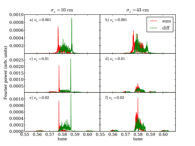
Figure 12: Simulated one-on-one bunch $y$ plane $\sigma$ and $\pi$ mode tune spectra for short bunches (a, c, e) and long bunches (b, d, f), for three different synchtrotron tunes, with a Tevatron-like lattice.

VI.3 Multi-bunch mode studies

When the Tevatron is running in its usual mode, each circulating beam contains 36 bunches. Every bunch in one beam interacts with every bunch in the opposite beam, though only two interaction points are useful for high energy physics running. The other 136 interaction points are unwanted and detrimental to beam lifetime and luminosity. The beam orbit is deflected in a helical shape by electrostatic separators to reduce the impact of these unwanted collisions, so the beams are transversely separated from each other in all but the two high-energy physics interaction points. Because of the helical orbit, the beam separation is different at each parasitic collision location. For instance, a bunch near the front of the bunch train will undergo more long-range close the the head-on interaction point, compared to a bunch near the rear of the bunch train. A particular bunch experiences collisions at specific interaction points with other bunches each of which has its own history of collisions. This causes bunch-to-bunch variation in disruption and emittance growth as will be demonstrated below.

We will begin the validation and exploration of the multi-bunch implementation starting with runs of two-on-two bunches and six-on-six bunches before moving on to investigate the situation with the full Tevatron bunch fill of 36-on-36 bunches. Two-on-two bunches will demonstrate the bunches coupling amongst each other, but will not be enough to demonstrate the end bunch versus interior bunch behavior that characterizes the Tevatron. For that, we will look at six-on-six bunch runs.

In these studies, we are only filling the ring with at most six bunches in a beam. Referring to Fig. 7, we see that only the head-on location at B0 is within the green shaded region where beam-beam collisions may occur with six bunches in each beam. Because of the beam-beam collisions, each bunch is weakly coupled to every other bunch which gives rise to multi-bunch collective modes.

We began the investigation of these effects with a simulation of beams with two bunches each. The bunches are separated by 21 RF buckets as they are are in normal Tevatron operations. Collisions occur at the head-on location and at parasitic locations 10.5 RF buckets distant on either side of the head-on location. To make any excited modes visible, we ran with $2.2\times 10^{11}$ particles, which gives a single bunch beam-beam parameter of $0.01$. There are four bunches in this problem. We label bunch 1 and 3 in beam 1 (proton) and bunch 2 and 4 in beam 2 (antiproton) with mean $y$ positions of the bunches $y_{1},\ldots y_{4}$. By diagonalizing the covariance matrix of the turn-by-turn bunch centroid deviations, we determine four modes, shown in Fig. 13. Fig. 13(a) shows the splitting of the $\sigma$ mode. The coefficients of the two modes indicate that this mode is primarily composed of the sum of corresponding beam bunches (1 with 2, 3 with 4) similar to the $\sigma$ mode in the one-on-one bunch case. The other two modes in Fig 13(b) have the character and location in tune space of the $\pi$ mode, from their coefficients and also their reduced strength compared to the $\sigma$ mode.

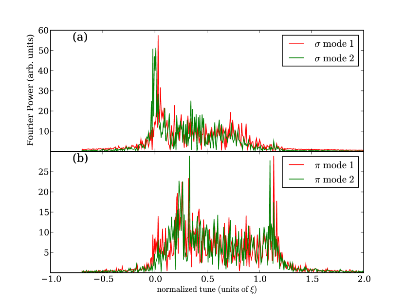
Figure 13: Mode tune spectrum for a two on two bunch run at $2.2\times 10^{11}$ particles/bunch ($\xi=0.01$). Figure (a) shows the two modes that are most like $\sigma$ modes. $\sigma$ mode 1 is $0.53y_{1}+0.53y_{2}+0.59y_{3}-0.31y_{4}$, $\sigma$ mode 2 is $0.39y_{1}+0.49y_{2}-0.46y_{3}-0.63y_{4}$. Figure (b) shows the two $\pi$-like modes. $\pi$ mode 1 is $0.74y_{1}-0.66y_{2}-0.08y_{3}$, $\pi$ mode 2 is $0.12y_{1}+0.20y_{2}-0.66y_{3}+0.31y_{4}$. The absolute scale of the Fourier power is arbitrary, but the relative scales of plots (a) and (b) are the same.

With six on six bunches, features emerge that are clearly bunch position specific. Fig. 14(a) shows the turn-by-turn evolution of 4D emittance and (b) $y$ kurtosis for each of the six proton bunches. It is striking that bunch 1, the first bunch in the sequence, has a lower emittance growth than all the other bunches. Emittance growth increases faster with increasing bunch number from bunches 2–5, but bunch 6 has a lower emittance growth than even bunch 4. The kurtosis of bunch 1 changes much less than that of any of the other bunches, but bunches 2–5 have a very similar evolution, while bunch 6 is markedly closer to bunch 1. One difference between the outside bunches (1 and 6) and the inside bunches (2–5) is that they have only one beam-beam interaction at the parasitic IP closest to the head-on collision, while the inside bunches have one collision before the head-on IP, and one after it. The two parasitic collision points closest to the head-on collision point have the smallest separation of any of the parasitics, so interaction there would be expected to disrupt the beam more than interactions at other parasitic locations.

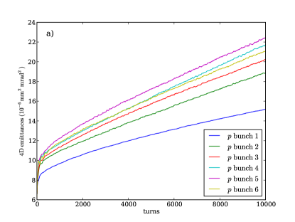
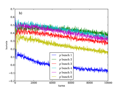
Figure 14: A six-on-six bunch Tevatron run with $8.8\times 10^{11}$ particles/bunch: (a) The turn-by-turn evolution of 4D emittance of each of the six bunches. (b) The turn-by-turn evolution of $y$ kurtosis of the six bunches.

To test this hypothosis, we did two additional runs. In the first, the beam separation at the parasitic IP immediately downstream of the head-on IP was artificially increased in the simulation so as to have essentially no effect. The effect of this is that the first proton bunch will not have any beam-beam collisions at an IP close to the head-on IP, while all the other bunches will have one collision at a near-head-on IP. The corresponding plots of emittance and kurtosis are shown in Fig. 15. The kurtosis data shows that bunches 2–5 which all suffer one beam-beam collision at a close parasitic IP are all together while bunch 1 which does not have a close IP collision is separated from the others.

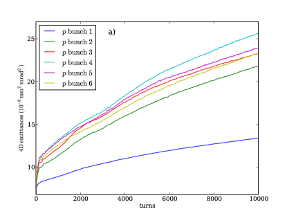
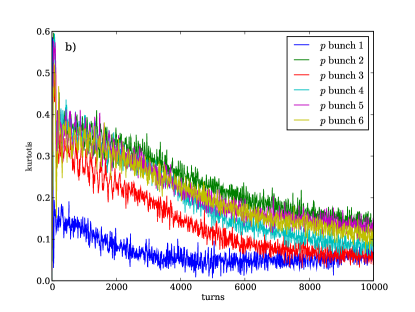
Figure 15: In a six-on-six bunch Tevatron run with $8.8\times 10^{11}$ particles/bunch, with the beam spacing at the first parasitic IP downstream of the head-on location artificially increased: (a) The 4D emittance of each of the six bunches as a function of turn. (b) the $y$ kurtosis of the six bunches as a function of turn.

Emittance and kurtosis growth in simulations where the beam separation at the closest upstream and downstream parasitic IPs was increased is shown in Fig. 16. In this configuration no bunch suffers a strong beam-beam collision at a parasitic IP close to the head-on location so the kurtosis of all the bunches evolves similarly.

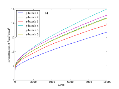
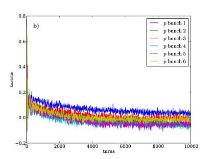
Figure 16: In a six-on-six bunch Tevatron run with $8.8\times 10^{11}$ particles/bunch, with the both nearest upstream and downstream parasitic IP artificially widened: (a) The 4D emittance of each of the six bunches as a function of turn. (b) the $y$ kurtosis of the six bunches as a function of turn.

VII Lower chromaticity threshold

During the Tevatron operation in 2009 the limit for increasing the initial luminosity was determined by particle losses in the so-called squeeze phase AVPAC09 . At this stage the beams are separated in the main interaction points (not colliding head-on), and the machine optics is gradually changed to decrease the beta-function at these locations from 1.5 m to 0.28 m.

With proton bunch intensities currently approaching $3.2\times 10^{11}$ particles, the chromaticity of the Tevatron has to be managed carefully to avoid the development of a head-tail instability. It was determined experimentally that after the head-on collisions are initiated, the Landau damping introduced by beam-beam interaction is strong enough to maintain beam stability at chromaticity of +2 units (in Tevatron operations, chromaticity is $\Delta\nu/({\Delta p}/p)$.) At the earlier stages of the collider cycle, when beam-beam effects are limited to long-range interactions the chromaticity was kept as high as 15 units since the concern was that the Landau damping is insufficient to suppress the instability. At the same time, high chromaticity causes particle losses which are often large enough to quench the superconducting magnets, and hence it is desireable to keep it at a reasonable minimum.

Table 1: Beam parameters for Tevatron simulation

Parameter	value
beam energy	$980\,\mbox{GeV}$
$p$ particles/bunch	$3.0\times 10^{11}$
$\bar{p}$ particles/bunch	$0.9\times 10^{11}$
$p$ tune $(\nu_{x},\nu_{y})$	(20.585,20.587)
$p$ (normalized) emittance	$20\pi\,\textrm{mm}\,\textrm{mrad}$
$\bar{p}$ tune $(\nu_{x},\nu_{y})$	(20.577,20.570)
$\bar{p}$ (normalized) emittance	$6\pi\,\textrm{mm}\,\textrm{mrad}$
synchrotron tune $\nu_{s}$	0.0007
slip factor	0.002483
bunch length (rms)	$43\,{\rm cm}$
$\delta p/p$ momentum spread	$1.2\times 10^{-4}$
effective pipe radius	$3\,{\rm cm}$

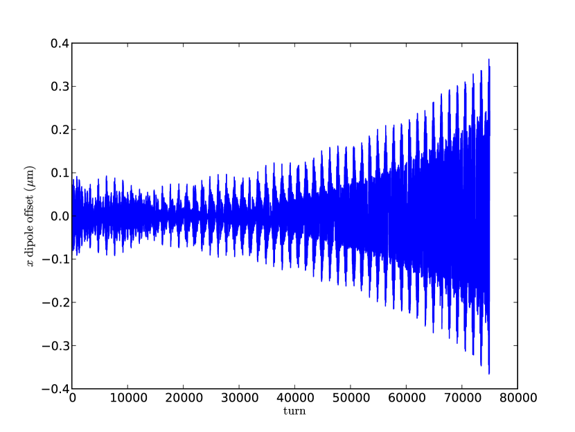
Figure 17: The x dipole moment in a simulation with $C=-2$ and no beam-beam effect showing the development of instability.

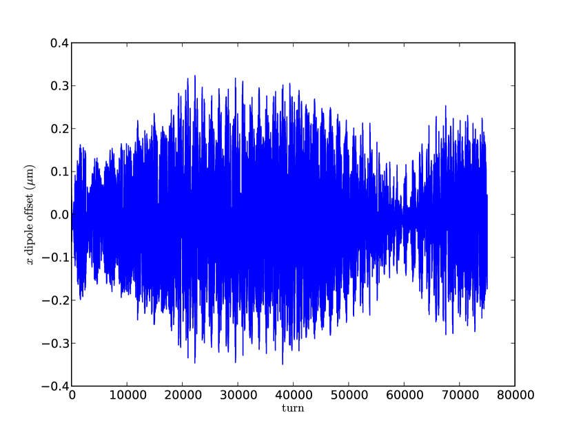
Figure 18: The x dipole moment of a representative bunch in a 36-on-36 simulation with $C=-2$ with beam-beam effects and beams separated showing no obvious instability within the limits of the simulation.

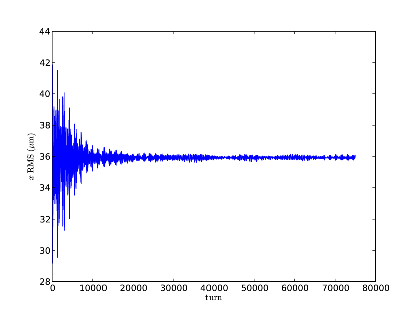
Figure 19: The x RMS moment of a representative bunch in a 36-on-36 simulation with $C=-2$ with beam-beam effects and beams separated showing no obvious instability within the limits of the simulation.

Our multi-physics simulation was used to determine the safe lower limit for chromaticity. The simulations were performed with starting beam parameters listed in Table 1. With chromaticity set to -2 units, and no beam-beam effect, the beams are clearly unstable as seen in Fig. 17. With beams separated, turning on the beam-beam effect prevents rapid oscillation growth during the simulation as shown in Fig. 18. The bursts of increased amplitude is sometimes indicative of the onset of instability, but it is not obvious within the limited duration of this run. The RMS size of the beam also does not exhibit any obvious unstable tendencies as shown in Fig. 19.

Based on these findings the chromaticity in the squeeze was lowered by a factor of two, and presently is kept at 8-9 units. This resulted in a significant decrease of the observed particle loss rates (see, e.g., Fig. 5 in AVPAC09 ).

VIII Summary

The key features of the developed simulation include fully three-dimentional strong-strong multi-bunch beam-beam interactions with multiple interaction points, transverse resistive wall impedance, and chromaticity. The beam-beam interaction model has been shown to reproduce the location and evolution of synchrobetatron modes characteristic of the 3D strong-strong beam-beam interaction observed in experimental data from the VEPP-2M collider. The impedance calculation with macroparticles excites both the strong and weak head-tail instabilities with thresholds and growth rates that are consistent with expectations from a simple two-particle model and Vlasov calculation. Simulation of the interplay between the helical beam-orbit, long range beam-beam interactions and the collision pattern qualitatively matches observed patterns of emittance growth.

The new program is a valuable tool for evaluation of the interplay between the beam-beam effects and transverse collective instabilities. Simulations have been successfully used to support the change of chromaticity at the Tevatron, demonstrating that even the reduced beam-beam effect from long-range collisions may provide enough Landau damping to prevent the development of head-tail instability. These results were used in Tevatron operations to support a change of chromaticity during the transition to collider mode optics, leading to a factor of two decrease in proton losses, and thus improved reliability of collider operations.

- (1) Run II handbook, http://www-bd.fnal.gov/runII
- (2) A. Valishev et al., “Observations and Modeling of Beam-Beam Effects at the Tevatron Collider”, PAC2007, Albuquerque, NM, 2007
- (3) M. Xiao et al., “Tevatron Beam-Beam Simulation at Injection Energy”, PAC2003, Portland, OR, 2003
- (4) Y. Alexahin, “On the Landau Damping and Decoherence of Transverse Dipole Oscillations in Colliding Beams”, Part. Acc. 59, 43 (1996)
- (5) E.A. Perevedentsev and A.A. Valishev, “Simulation of Head-Tail Instability of Colliding Bunches”, Phys. Rev. ST Accel. Beams 4, 024403, (2001)
- (6) J. Qiang, M.A. Furman, R.D. Ryne, J.Comp.Phys., 198 (2004), pp. 278–294, J. Qiang, M.A. Furman, R.D. Ryne, Phys. Rev. ST Accel. Beams, 104402 (2002).
- (7) V. Lebedev, http://www-bdnew.fnal.gov/pbar/ organizationalchart/lebedev/OptiM/optim.htm
- (8) A. Valishev et al., “Progress with Collision Optics of the Fermilab Tevatron Collider”, EPAC06, Edinburgh, Scotland, 2006
- (9) A. Chao, Physics of Collective Beam Instabilities in High Energy Accelerators., pp. 56–60, 178–187, 333-360 John Wiley and Sons, Inc., (1993)
- (10) A. Piwinski, IEEE Trans. Nucl. Sci. NS-26 (3), 4268 (1979).
- (11) K. Yokoya, Phys. Rev. ST-AB 3, 124401 (2000).
- (12) I.N. Nesterenko, E.A. Perevedentsev, A.A. Valishev, Phys.Rev.E, 65, 056502 (2002)
- (13) E.A. Perevedentsev and A.A. Valishev, Phys. Rev. ST Accel. Beams 4, 024403 2001 ; in Proceedings of the 7th European Particle Accelerator Conference, Vienna, 2000 unpub- lished , p. 1223; http://accelconf.web.cern.ch/AccelConf/e00/ index.html
- (14) V.V. Danilov and E.A. Perevedentsev, Nucl. Instrum. Methods Phys. Res. A 391, 77 1997 .
- (15) A. Chao, Physics of Collective Beam Instabilities in High Energy Accelerators., Figure 4.8 on p. 183, John Wiley and Sons, Inc., (1993).
- (16) A. Chao, Physics of Collective Beam Instabilities in High Energy Accelerators., p. 9, John Wiley and Sons, Inc., (1993)
- (17) D.A. Edwards and M.J. Syphers, An Introducution to the Physics of High Energy Accelerators, pp. 30–46, John Wiley and Sons Inc., 1993.
- (18) A. Chao, Physics of Collective Beam Instabilities in High Energy Accelerators., p. 351, John Wiley and Sons, Inc., (1993).
- (19) F.W. Jones, W. Herr, T. Pieloni, Parallel Beam-Beam Simulation Incorporating Multiple Bunches and Multiple Interaction Regions, THPAN007 in Proceedings of PAC07, Albuquerque, NM (2007), T. Pieloni, W. Herr, Models to Study Multi Bunch Coupling Through Head-on and Long-range Beam-Beam Interactions, WEPCH095 in Proceedings of EPAC06, Edinburgh, Scotland, (2006), T. Pieloni and W. Herr, Coherent Beam-beam Modes in the CERN Large Hadron Collider (LHC) for Multiple Bunches, Different Collision Schemes and Machine Symmetries, TPAT078 in Proceedings of PAC05, Knoxville, TN, (2005).
- (20) V. Shiltsev, et al., “Beam-Beam Effects in the Tevatron,” PRSTAB, 8, 101001 (2005).
- (21) A. Valishev et al., “Recent Tevatron Operational Experience”, PAC2009, Vancouver, BC, 2009