Intrinsic torsion classes of
Riemannian structures

Abstract

This article introduces the notion of intrinsic torsion varieties associated to $G$-structures on a parallelizable Riemannian manifold. As an illustration, the intrinsic torsion varieties of orthogonal almost product structures are analysed on the Iwasawa manifold.

Introduction

Determining integrability of a geometrical structure is a fundamental problem in differential geometry. A suitable formulation relates the equivalence problem for $G$-structures with the theory of $k$-jets. In this context, the intrinsic torsion of a $G$-structure is a first-order obstruction to integrability. In certain circumstances, vanishing of the intrinsic torsion is not only a necessary but also a sufficient integrability condition. The celebrated Darboux and Newlander–Nirenberg theorems assert exactly this for almost symplectic and almost complex structures respectively. On the other hand, in the Riemannian situation, non-vanishing intrinsic torsion impedes a reduction of the holonomy group.

Symmetry properties of the intrinsic torsion tensor $\tau$ have been exploited in various cases for classifying manifolds with $G$-structure. The prototype classification is given by Gray and Hervella in [7], and regards almost Hermitian and almost symplectic manifolds. Later in [11], Naveira applied analogous approach to the classification of almost product manifolds, Cabrera and Swann studied the case of quaternion-Hermitian manifolds [4] etc. Applications of a Gray–Hervella type classification intervene in the construction of specific $G_{2}$-structures on 7-manifolds (see [5]). Constructions of symplectic and other structures of special classes are described in [6] and in other articles by Salamon, Fino, Chiossi and others.

In this article we consider a manifold $M$ with a fixed Riemanian metric and subgroup $G$ of $O(N)$. Different $G$-reductions of the Riemannian structure are parametrized by a suitable space.

A favorable context to start our analysis is the case in which $M$ is a nilmanifold. Nilmanifolds are parallelizable in a natural way, their geometry reflects properties of the underlying nilpotent algebra in terms of invariant tensors. An invariant $G$-structure becomes a point of the homogeneous space $O(N)/G$, and this space contains the subsets parameterizing special $G$-structures as real subvarieties. These are the intrinsic torsion varieties (ITV’s) associated to the problem.

In the first section, we introduce the precise definition of ITV’s. In the rest of the article we analyse a specific case, namely the classification of orthogonal almost product structures on the Iwasawa manifold. Similar analysis on almost Hermitian structures (using different methods) has been developed in [1]. The method described in the present article exploits essentially basic definitions and so appears more general. The rich geometry of the ITV’s highlighted in these cases (by rather simple calculations) motivates the research of a general theory which explains the variation of the intrinsic torsion of distinguished reductions of a $G$-structure.

1 Intrinsic torsion varieties

The restriction of the canonical soldering form $\theta$ on the frame bundle $LM$ of a smooth manifold to a $G$-structure $P$ allows one to view the tangent space in each point of $M$ as a representation $\rho_{P}$ of $G$ on $\mathbb{R}^{n}$. The covariant derivative $\nabla_{\phi}\theta$ associated to a connection $\phi$ on $LM$ defines a horizontal torsion form $\Theta$, with values in $\mathrm{Hom}(\mathbb{R}^{n}\wedge\mathbb{R}^{n},\mathbb{R}^{n})$. The structure function on $P$ represents, the component of $\Theta$ independent of the choice of connection compatible with the structure, i.e. the image of $\Theta$ in the space

$$\mathscr{W}=\mathrm{Hom}(\mathbb{R}^{n}\wedge\mathbb{R}^{n},\mathbb{R}^{n})/\alpha(\mathrm{Hom}(\mathbb{R}^{n},\mathfrak{g})).$$ (1)

Here $\alpha$ is the skew-symmetrization in $\mathrm{Hom}(\mathbb{R}^{n},\mathfrak{g})$, and $\mathfrak{g}$ is the Lie algebra of $G$. The structure function defines over $M$ a section $\tau$ of a vector bundle with fibre (1) called the intrinsic torsion of $P$. The variation of $\Theta$ along a fibre of $P$ defines a representation $\rho_{P}$ on $\mathscr{W}$. If at a point $p\in P$ $\Theta$ belongs to a $\rho_{P}$-submodule $\mathscr{U}$, in the projected point $\tau$ belongs to the same subspace. Equivalently, we say that $\tau$ maps to zero in the quotient $\mathscr{W}/\mathscr{U}$. Adopting the expression coined in [9]:

Definition 1.

A null-torsion structure on a manifold is a $G$-structure for which $\tau$ belongs to a proper $G$-submodule $\mathscr{U}$ of $\mathscr{W}$.

The space (1) decomposes into a direct sum of $G$-irreducible subspaces $\mathscr{W}_{i}$. A classification of $G$-structures based on criteria whereby $\tau$ belongs to a specific subset of these components appears “natural” as $\Theta$ is basic tensorial form and “geometrically relevant” as the obstructions determined by the intrinsic torsion reduce to a specific subspace of $\mathscr{W}$.

Consider a fixed Riemannian manifold $M$. For $O(N)$, the space (1) is trivial, and the consequent vanishing of the structure function explains the existence of a canonical (Levi-Civita) torsion-free connection $\phi_{LC}$. Let $G$ be a closed subgroup of $O(N)$. A reduction to a $G$-structure $P_{\xi}$ can be defined by detecting $G$ as the stabilizer $Satb(\xi)$ of a tensor $\xi$. The parameter space of such reductions can be point-wise identified with the $O(N)$-orbit $\mathscr{O}_{\xi}$ of $\xi$, so a $G$-structure on $M$ is a smooth section of a bundle with fibre $\mathscr{O}\cong O(N)/G$.

The torsion of the reduced structure comes from the restriction of $\theta$ to $P_{\xi}$ eliminating the dependence of $\nabla\theta$ on connections compatible with $P_{\xi}$. In general, the Levi-Civita connection does not reduce to $P_{\xi}$, so $\tau_{\xi}$ does not vanish. This incompatibility arises from the non-zero projection onto $\mathfrak{g}^{\bot}_{\xi}$ (the orthogonal complement of $\mathfrak{g}_{\xi}$ inside the vertical space of $P$) of a vector horizontal with respect to $\phi_{LC}$. In other words, $\tau_{\xi}$ depends on the mutual positions of the horizontal spaces of $\phi_{LC}$ and the connections compatible with $P_{\xi}$. For this reason in the Riemannian case:

$$\mathscr{W}\cong\mathbb{R}^{n}\otimes\mathfrak{g}^{\bot}_{\xi}.$$ (2)

Fact: Reductions of an $O(N)$-structure may belong to different null-torsion classes.

This fact has been remarked in [1, 9]. We can consider a “local problem” i.e. given a small open neighborhood of a point on $M$ (using a single coordinate chart domain), determine the mechanism which causes the class-variation of $\tau_{\xi}$ between distinguished reductions of $P$.

Consider a Riemannian reduction $P_{\xi}$. A well-known fact is that:

$$\mathrm{Stab}(g\xi)=g\kern 2.0pt\kern 2.0pt\mathrm{Stab}(\xi)\kern 2.0pt\kern 2.0ptg^{-1},\kern 2.0pt\kern 2.0pt\kern 2.0pt\kern 2.0pt\kern 2.0ptg\in O(N).$$ (3)

Given a decomposition $\mathscr{W}=\oplus_{i}\mathscr{W}_{i}$, the action of $g\in O(N)$ transforms it in $\oplus_{i}g\mathscr{W}_{i}$. In fact given $h\in\mathrm{Stab}(\xi)$, suppose $\tau_{\xi}\in\mathscr{W}_{i}$. As $(ghg^{-1})(g\mathscr{W}_{i})=g(h\mathscr{W}_{i})$, $ghg^{-1}$ acts on $g\mathscr{W}_{i}$ as $h$ acts on $\mathscr{W}$. So $P_{\xi}$ and $P_{g\xi}$ belong to the same class if:

$$\tau_{\xi}\in\oplus_{i}\mathscr{W}_{i}\kern 2.0pt\kern 2.0pt\kern 2.0pt\kern 2.0pt\kern 2.0ptand\kern 2.0pt\kern 2.0pt\kern 2.0pt\kern 2.0pt\kern 2.0pt\tau_{g\xi}\in\oplus_{i}g\mathscr{W}_{i}$$ (4)

The mere $O(N)$-action on the fibres on $P$ keeps $\tau_{\xi}$ in the same submodule.

The Levi-Civita connection form restricted to $P_{\xi}$ can be written as

$$\phi_{LC}=\phi_{\xi}+\psi_{\xi}.$$

Here $\phi_{\xi}$ is a connection compatible with $P_{\xi}$ and $\psi_{\xi}$ represents the projection on the specific orthogonal complement $\mathfrak{g}^{\bot}_{\xi}$. Along a fibre of $P$ the form $\phi_{LC}$ varies via the adjoint representation of $O(N)$ and the variation of the splitting $\mathfrak{g}_{\xi}\oplus\mathfrak{g}^{\bot}_{\xi}$ follows the rule (3). This implies that $Ad_{g}\phi_{\xi}$ defines point-wise a connection compatible with $P_{g\xi}$. As we just project on the subspaces of the splitting, the variation of $\psi_{\xi}$ along the vertical directions transversal to the fibres of $P_{\xi}$ is determined to first order by the $O(N)$-action. So apparently the variation of all elements (the representation on $\mathscr{W}$ and the obstruction $\psi$) is determined by the $O(N)$-action. But this cannot justify the null-torsion class variation. This means that a point-wise first-order $G$-structure theory approach cannot explain this phenomenon. The mechanism, which induces the “jumps” of the reductions from one class to another should be expressed in terms a higher-order prolongation of $P$. This consideration appears quite natural in the context of the theory of prolongations of $G$-structures (see for example [13]). In fact the splitting of the tangent space in each point of $P$ determines a $G$-structure over the total space of the $P$ i.e. a prolongation. In [9] has been already underlined the relation between the intrinsic torsion and the second fundamental form of the embedding $P_{\xi}\subset P$, which contains more information.

A problem closely related to the local-one appears when $M$ is a parallelizable manifold. If we declare a global section $s$ of the frame bundle to be orthonormal, we define a Riemannian metric on $M$. The bundle of orthonormal frames is a product $M\times O(N)$. We call a $G$-structure invariant if (relative to the parallelization $s$) $\xi$ is constant. Invariant $G$-structures are parametrized by a single classifying orbit $\mathscr{O}$.

Definition 2.

Intrinsic torsion variety (ITV) is a subset of $\mathscr{O}=O(N)/G$ composed by invariant reductions which belong to a given null-torsion class.

Problem: Analyse the geometry of the Intrinsic Torsion Varieties of invariant structures on a parallelizable Riemannian manifold.

Each point $\xi$ in $\mathscr{O}$ defines an invariant reduction $P_{\xi}$, and determines both, the intrinsic torsion $\tau_{\xi}$ and the $G$-representation on the space (1). The intrinsic torsion can be regarded as a map from $\mathscr{O}$ to $\mathscr{W}$. The $G$-representation on $\mathscr{W}$ varies over $\mathscr{O}$ by (3). Equation (4) suggests a special class of ITV’s, namely constant torsion varieties (CTV’s) can be defined by the condition:

$$\tau_{g\xi}=g\tau_{\xi}.$$ (5)

The $O(N)$-action on the tensor components can be expressed in terms of polynomials, so $\xi\longrightarrow g\xi$ and $\tau_{\xi}\longrightarrow g\tau_{\xi}$ are polynomial functions. This means that CTV’s can be described as zero-sets of polynomial functions on $\mathscr{O}$ and so CTV’s are varieties in some general algebraic sense. This observation, involving invariant polynomial functions, suggests that tools of Geometric Invariant Theory can be applied to the study of ITV’s. The key point of the general description of ITV’s is the variation of the intrinsic torsion “transversal” to the $O(N)$ action.

Remark 3.

We expect that an ITV is fibration of algebraic CTV’s over a “cross section” in the set of $O(N)$ orbits in $\mathscr{W}$.

2 Almost product structures

Consider a smooth section $\mathfrak{F}$ of the tensor bundle $T^{*}M\otimes TM$ over a differentiable manifold. The “value” in $p$ of $\mathfrak{F}$ is an endomorphism of $T_{p}M$. If $\mathfrak{F}$ is stabilized by a subgroup $G$ of $GL(N,\mathbb{R})$, it defines a $G$-structure on $M$. The action of $\mathfrak{F}_{p}$ can be analysed in terms of its eigenspaces which give rise to vector distributions in $TM$. The integrability of these distributions characterizes $M$. Almost complex, $f$-structures [2, 14], mixed structures [9, 10] etc. are relevant examples.

The almost product structures (APS’s) introduced by Naveira in [11] can be included in this setup. An APS corresponds to a splitting of the tangent space at each point of $M$ into a direct sum of vertical and horizontal subspaces $T_{p}M=\mathcal{V}\oplus\mathcal{H}$. Denoting by $\mathfrak{v},\mathfrak{h}$ the projections on $\mathcal{V}$ and $\mathcal{H}$, an APS can be defined stabilizing:

$$\mathfrak{P}=\mathfrak{v}-\mathfrak{h}\kern 2.0pt\kern 2.0pt\kern 2.0pt\in\kern 2.0pt\kern 2.0pt\kern 2.0ptT^{*}M\otimes TM.$$ (6)

An orthogonal almost product structure (OPS) is a reduction of a Riemannian structure with group $O(p)\times O(q)$, $\mathcal{V}$ and $\mathcal{H}$ are orthogonal subspaces. The same splitting regards the cotangent space and the summands $\mathcal{V}$ and $\mathcal{H}$ can be identified with their dual spaces via the metric. The parameter space of these reductions is the Grassmannian of $p$-planes in $\mathbb{R}^{N}$.

The intrinsic torsion of an OPS is given by the Levi-Civita derivative $\nabla\mathfrak{P}$, equivalently by the Levi-Civita derivative of the covariant 2-tensor $\Phi=g(\mathfrak{P}\kern 2.0pt\kern 2.0pt\kern 2.0pt,\kern 2.0pt\kern 2.0pt\kern 2.0pt)$. As

$$\mathfrak{so}(N)\ \cong\ \Lambda^{2}(\mathcal{V}\oplus\mathcal{H})=\Lambda^{2}\mathcal{V}\oplus\Lambda^{2}\mathcal{H}\\ \oplus(\mathcal{V}\wedge\mathcal{H})\cong\mathfrak{so}(p)\oplus\mathfrak{so}(q)\oplus(\mathcal{V}\otimes\mathcal{H}),$$

the space of intrinsic torsion (2) is:

$$\mathbb{R}^{N}\otimes\mathfrak{g}^{\perp}\cong(\mathcal{V}\oplus\mathcal{H})\otimes(\mathcal{V}\otimes\mathcal{H}).$$ (7)

OPS’s has been classified by Naveira in [11] by means of the following $O(p)\times O(q)$-irreducible components of the intrinsic torsion space (7):

$$\begin{array}[]{lll}\mathscr{W}_{1}=\Lambda^{2}\mathcal{V}\otimes\mathcal{H},\kern 2.0pt\kern 2.0pt&\mathscr{W}_{2}=S_{0}^{2}\mathcal{V}\otimes\mathcal{H},\kern 2.0pt\kern 2.0pt&\mathscr{W}_{3}=Tr(\mathcal{V}\otimes\mathcal{V})\otimes\mathcal{H},\\ \mathscr{W}_{4}=\Lambda^{2}\mathcal{H}\otimes\mathcal{V},\kern 2.0pt\kern 2.0pt&\mathscr{W}_{5}=S_{0}^{2}\mathcal{H}\otimes\mathcal{V},\kern 2.0pt\kern 2.0pt&\mathscr{W}_{6}=Tr(\mathcal{H}\otimes\mathcal{H})\otimes\mathcal{V}.\end{array}$$ (8)

The null-torsion conditions detect thirty-six classes of OPS’s obtained by summing two or more of these subspaces and exchanging “vertical” and “horizontal”.

Let $v$ denote a section of the distribution $\mathcal{V}$. The Levi-Civita connection on $P$ defines a connection on the vector bundle $\mathcal{V}$ via the projections of $\nabla v$ on $\mathcal{V}$. Vice versa the incompatibility of the Levi-Civita connection with an OPS is determined by the projection of $\nabla v$ on $\mathcal{H}$. More precisely:

Theorem 4.

The intrinsic torsion of an OPS is completely determined by the maps:

$$\tau_{v}:\mathcal{V}\to\mathcal{H}\otimes\mathcal{H},\kern 2.0pt\kern 2.0pt\kern 2.0pt\kern 2.0pt\kern 2.0pt\kern 2.0pt\tau_{h}:\mathcal{H}\to\mathcal{V}\otimes\mathcal{V}$$

defined by the orthogonal projections of $\nabla v$ on $\mathcal{H}\otimes\mathcal{H}$ and $\nabla h$ onto $\mathcal{V}\otimes\mathcal{V}$.

Proof. We take an orthonormal basis of forms $\{v^{i},h^{j}\}$, and express $\Phi$ as:

$$\Phi=\sum_{i=1}^{p}v^{i}\otimes v^{i}-\sum_{j=1}^{q}h^{j}\otimes h^{j}$$

Thus $\nabla_{w}\Phi$ with $w\in TM$ is determined by terms of the form:

$$\sum_{i=1}^{p}(\nabla_{w}v^{i})\otimes v^{i}-\sum_{j=1}^{q}(\nabla_{w}h^{i})\otimes h^{i}$$ (9)

The tensor $\Phi$ restricted to $\mathcal{V}$ and $\mathcal{H}$ is proportional to the metric. This implies $\nabla_{x}\Phi(y,z)=0$ for each $x\in TM$ if $y$ and $z$ are both vertical or horizontal. The non-zero contributions of $\nabla_{w}v^{i}$ and $\nabla_{w}h^{i}$ to (9) belong respectively to $\mathcal{H}$ and $\mathcal{V}$ and (9) belongs to the space $(\mathcal{V}\oplus\mathcal{H})\mathcal{V}\mathcal{H}$. So setting $w=\sum_{k=1}^{p}a_{k}v_{i}+\sum_{l=1}^{q}b_{l}h_{l}$, we re-write (9) as:

$$\begin{array}[]{l}\sum_{i=1}^{p}\sum_{k=1}^{p}a_{k}(\nabla_{v_{k}}v^{i})\otimes v^{i}+\sum_{i=1}^{p}\sum_{l=1}^{q}b_{l}(\nabla_{h_{l}}v^{i})\otimes v^{i}-\\ \kern 2.0pt\kern 2.0pt\kern 2.0pt\kern 2.0pt\kern 2.0pt\kern 2.0pt\kern 2.0pt\kern 2.0pt\kern 2.0pt\kern 2.0pt\kern 2.0pt\kern 2.0pt\kern 2.0pt\kern 2.0pt\kern 2.0pt\kern 2.0pt\kern 2.0pt\kern 2.0pt\kern 2.0pt\kern 2.0pt\kern 2.0pt\kern 2.0pt\kern 2.0pt\kern 2.0pt\kern 2.0pt\kern 2.0pt\kern 2.0pt\kern 2.0pt\kern 2.0pt\kern 2.0pt\kern 2.0pt\kern 2.0pt\kern 2.0pt\kern 2.0pt\kern 2.0pt\kern 2.0pt\kern 2.0pt\kern 2.0pt\sum_{j=1}^{q}\sum_{k=1}^{p}a_{i}(\nabla_{v_{i}}h^{j})\otimes h^{j}-\sum_{j=1}^{q}\sum_{l=1}^{q}b_{l}(\nabla_{h_{l}}h^{j})\otimes h^{j}.\end{array}$$

Compare now the first term, say $I$, (which belongs to $\mathcal{V}\otimes\mathcal{H}\otimes\mathcal{V}$) to the third term $III$ (which belongs to $\mathcal{V}\otimes\mathcal{V}\otimes\mathcal{H}$). Let us write $I$ (respectively $III$) in terms of the basis $\{h^{j}\}$ (respectively $\{v^{i}\}$):

$$\begin{array}[]{rl}I&=\sum_{i=1}^{p}\sum_{k=1}^{p}a_{k}\sum_{n=1}^{q}(\nabla_{v_{k}}v^{i},h^{n})h^{n}\otimes v^{i}\\ -III&=\sum_{j=1}^{q}\sum_{k=1}^{p}a_{i}\sum_{m=1}^{p}(\nabla_{v_{i}}h^{j},v^{m})v^{m}\otimes h^{j}\end{array}$$

As $g(v,h)=0$ and $\nabla g=0$ we have $(\nabla_{w}v,h)=-(v,\nabla_{w}h)$, so:

$$\begin{array}[]{rl}I&=\sum_{i=1}^{p}\sum_{k=1}^{p}a_{k}\sum_{n=1}^{q}(h^{n},\nabla_{v_{k}}v^{i})h^{n}\otimes v^{i}\\ III&=\sum_{j=1}^{q}\sum_{k=1}^{p}a_{i}\sum_{m=1}^{p}(h^{j},\nabla_{v_{i}}v^{m})v^{m}\otimes h^{j}\end{array}$$

as the order of the summations and the names of the indices are irrelevant, these terms are equivalent from the point of view of the representation. The same consideration applied to the second and the fourth term completes the proof.∎

As the vertical space $\mathfrak{so}(n)\cong\Lambda^{2}T_{p}$, a suitable starting point for the general analysis of ITV’s might be the Riemannian $G$-reductions defined by stabilizing a $2$-form. In the case of an (oriented) Riemannian manifold “contraction” of a $2$-form with the metric determines skew-symmetric endomorphisms $\mathfrak{F}_{p}$. We can define an OPS by setting $\mathcal{V}=\mathrm{Im}\mathfrak{F}_{p},\mathcal{H}=\mathrm{ker}\mathfrak{F}_{p}$. In particular a simple $2$-form (one which with a suitable basis can be written as $e\wedge f$ with $e$ and $f$ $1$-forms) determines a reduction of the structure group to $SO(2)\times O(N-2)$.

In [1] the Gray–Hervella classes of invariant Hermitian structures on real six-dimensional nilmanifolds were embedded in $\mathbb{CP}^{3}$. The null-torsion conditions has been re-formulated in terms of differential, Hodge star operator and wedge product. This approach fails in our case. Consider $SO(2)\times SO(4)$ structures on $\mathbb{R}^{6}$.

$$d\alpha\in\begin{array}[]{rcl}\Lambda^{3}(\mathbb{R}^{6})^{*}\ =\ \Lambda^{3}(\mathcal{V}\oplus\mathcal{H})&\cong&\Lambda^{2}\mathcal{V}\kern 2.0pt\mathcal{H}\oplus\mathcal{V}\kern 2.0pt\Lambda^{2}\mathcal{H}\oplus\Lambda^{3}\mathcal{H}\end{array},$$ (10)

where $\alpha$ is the simple $2$-form. A “complementary” simple 4-form is $\beta=\ast\alpha$. Then

$$d\beta\ \in\ \Lambda^{5}(\mathbb{R}^{6})\kern 2.0pt\cong\mathcal{V}\oplus\mathcal{H}.$$ (11)

Comparing (7) and (8) to (10) and (11), we conclude that, between them, $d\alpha$ and $d\beta$ determine only four of the six irreducible components of intrinsic torsion. In [3] a subgroup $G$ of $GL(n,R)$ is called admissible if $G$ is the largest subgroup that fixes the space $\Lambda^{\ast}(\mathbb{R}^{N})^{G}$ of invariant forms on $\mathbb{R}^{n}$, $G$ is strongly admissible if, on $G$-structures, the closedness of the invariant forms is (point wise) equivalent to the vanishing of the intrinsic torsion.

3 Invariant SO(4)$\times$SO(2) structures on the Iwasawa manifold

The Iwasawa manifold $\mathscr{I}$ is the set of right cosets of the complex Heisenberg group over a lattice. So $\mathscr{I}$ is a complex manifold. As a real manifold $\mathscr{I}$ admits a left-invariant basis of real 1-forms $e^{i}$ such that:

$$de^{1}=0,\kern 2.0pt\kern 2.0pt\kern 2.0ptde^{2}=0,\kern 2.0pt\kern 2.0pt\kern 2.0ptde^{3}=0,\kern 2.0pt\kern 2.0pt\kern 2.0ptde^{4}=0,\kern 2.0pt\kern 2.0pt\kern 2.0ptde^{5}=e^{13}+e^{42},\kern 2.0pt\kern 2.0pt\kern 2.0ptde^{6}=e^{14}+e^{23}$$ (12)

where $e^{ij}=e^{i}\wedge e^{j}$. The Heisenberg group is 2-step nilpotent. The real geometry of $\mathscr{I}$ reflects the natural decomposition of $\mathfrak{g}^{*}=\mathscr{K}\oplus\langle e^{5},e^{6}\rangle$, where:

$$\mathscr{K}=\ker(d|\mathfrak{g}^{*}).$$

The map $\pi:G_{H}\to\mathbb{C}^{2}$ defined for $g\in G_{H}$ by $g\to(z^{1},z^{2})$ induces a fibration $\mathscr{I}\to T^{4}$ with fibre $T^{2}$. The space tangent to the fibre is $\mathscr{K}^{\bot}=\langle e_{5},e_{6}\rangle$. The fact that $\mathscr{I}$ is a $2$-torus bundle over a $4$-torus reflects a general property of nilmanifolds, their geometry can be understood in terms of tower of toric fibrations.

An invariant tensor on $\mathscr{I}$ can be expressed in terms of the bases $\mathrm{e}^{i}$ and $e_{i}$ with constant coefficients. Declaring $e^{i}$ are orthonormal, we determine an invariant Riemannian metric on $\mathscr{I}$. An invariant $SO(2)\times SO(4)$-structure is determined by an invariant simple $2$-form. These OPS’s are parametrized by the Grassmannian $\mathbb{G}\mathrm{r}_{2}(\mathbb{R}^{6})$. We single out a generic $2$-plane in $\mathbb{R}^{6}$ by a couple of orthogonal unit $1$-forms $v^{1}$ and $v^{2}$, or equivalently by the simple $2$-form $\omega=v^{1}\wedge v^{2}$. Obviously such a parametrization of the Grassmannian is $SO(2)$-overabundant.

We can apply the Frobenius Theorem for establishing the integrability of the distributions of an $SO(2)\times SO(4)$-structure on $\mathscr{I}$:

Proposition 5.

Given on $\mathscr{I}$ an orthonormal basis of vector fields $\{h_{i}\}$,

1) the distribution $\langle h_{1},...,h_{4}\rangle$ is integrable if and only if $d(h^{56})=0$

2) the distribution $\langle h_{1},h_{2}\rangle$ is integrable if and only if $d(h^{3456})=0$.

Proof. A tangent distribution $V\subset TM$ is integrable if and only if its annihilator $V^{\circ}\subset\Omega^{1}M$ generates a differential ideal. Consider $V^{\circ}=\langle v^{1},v^{2}\rangle$.

$$dv^{1}=v^{1}\wedge\alpha+v^{2}\wedge\beta,\qquad dv^{2}=v^{1}\wedge\alpha^{\prime}+v^{2}\wedge\beta^{\prime},$$

and so

$$d(v^{1}\wedge v^{2})=(v^{1}\wedge v^{2})\wedge\gamma$$ (13)

for some 1-form $\gamma$. The nilpotency condition forces $d(v_{1}\wedge v_{2})=0$. We can set:

$$\omega=v^{1}\wedge v^{2}=f^{1}\wedge f^{2}+f^{3}\wedge e^{5}+f^{4}\wedge e^{6}+ae^{56}$$ (14)

with $f^{1},...,f^{4}\in\mathscr{K}$, then (13) becomes:

$$d\omega=f^{3}\wedge e^{13}+f^{3}\wedge e^{42}+f^{4}\wedge e^{14}+f^{4}\wedge e^{23}+a(e^{514}+e^{523}+e^{613}+e^{642})$$ (15)

$$=f^{12}\wedge\gamma+f^{3}\wedge e^{5}\wedge\gamma+f^{4}\wedge e^{6}\wedge\gamma+ae^{56}\wedge\gamma$$

The lack of $f^{12}$ term on the left side forces $\gamma$ to be a linear combination of $f^{1}$ and $f^{2}$. If $a\neq 0$, the same consideration applied to the $e^{56}$-term shows that $\gamma$ is a linear combination of $e^{5}$ and $e^{6}$, which is a contradiction. If $a=0$,

$$f^{3}\wedge(e^{13}+e^{42})=f^{3}\wedge e^{5}\wedge\gamma\kern 2.0pt\kern 2.0pt\kern 2.0pt\kern 2.0pt\kern 2.0pt,\kern 2.0pt\kern 2.0pt\kern 2.0pt\kern 2.0pt\kern 2.0ptf^{4}\wedge(e^{14}+e^{23})=f^{3}\wedge e^{6}\wedge\gamma$$

which again contradicts the above condition. We conclude that the equality (15) cannot be realized except in the case $v_{1},v_{2}\in\mathscr{K}$ when both sides are zero. On a nilmanifold, analogous argument works for any subspace with annihilator whose generators define a simple $k$-form with $k\geq 2$. This includes the second item.∎

Obviously from (15) follows that for a simple $2$-form $\omega$:

$$d\omega=0\kern 2.0pt\kern 2.0pt\kern 2.0pt\kern 2.0pt\Leftrightarrow\kern 2.0pt\kern 2.0pt\kern 2.0pt\kern 2.0pt\omega\in\Lambda^{2}\mathscr{K}.$$ (16)

In this light we determine the set of OPS’s characterized by closed $4$-form complementary to the 2-form in (14). The simple $4$-form in question equals

$$\ast\omega=g^{34}\wedge e^{56}-g^{234}\wedge e^{6}-g^{134}\wedge e^{5}+g^{1234},$$ (17)

in terms of suitable 1-forms $g^{i}$. The last term gives no contribution to $d\ast\omega$, so there is no constraint on the $e^{56}$-component of $\omega$. Furthermore we have

$$d(g^{234}\wedge e^{6})=g^{234}\wedge(e^{14}+e^{23})=0,\kern 2.0pt\kern 2.0pt\kern 2.0pt\kern 2.0pt\kern 2.0pt\kern 2.0pt\kern 2.0ptd(g^{134}\wedge e^{5})=g^{134}\wedge(e^{13}+e^{42})=0,$$

these terms being $5$-forms on a four-dimensional space. Finally,

$$d(g^{34}\wedge e^{56})=g^{34}\wedge(e^{13}+e^{42})\wedge e^{6}-g^{34}\wedge e^{5}\wedge(e^{14}+e^{23}).$$

The vanishing of $d\ast\omega$ is now seen to be equivalent to the equations:

$$g^{34}\wedge\beta_{2}=0,\qquad g^{34}\wedge\beta_{3}=0,$$ (18)

where $\beta_{i}$ is the following basis of the space $\Lambda^{2}_{+}\mathscr{K}$ of self-dual 2-forms on $\mathscr{K}$.

$$\beta_{1}=e^{12}+e^{34},\kern 2.0pt\kern 2.0pt\kern 2.0pt\kern 2.0pt\kern 2.0pt\beta_{2}=e^{13}+e^{42},\kern 2.0pt\kern 2.0pt\kern 2.0pt\kern 2.0pt\kern 2.0pt\beta_{3}=e^{14}+e^{23}$$ (19)

Any simple $2$-form $\gamma\in\Lambda^{2}(\mathbb{R}^{4})^{*}$ can be written as $\gamma=\sigma+\tau$ with $\sigma\in\Lambda_{-}^{2}$ and $\tau\in\Lambda_{+}^{2}$ of equal norm. If $\gamma=g^{34}$, Equation (18) forces $\sigma=\pm\beta_{1}$, so we obtain:

$$g^{34}=\pm\beta_{1}+\tau,$$ (20)

where $\tau$ is any unit element of $\Lambda^{2}_{-}$. Such 2-forms in $\Lambda^{2}\mathscr{K}$ represent oriented real planes $\left<v,J_{1}v\right>$ or $\left<v,-J_{1}v\right>$ invariant under the action of the complex structure $J_{1}$ associated to the $2$-form $\beta_{1}$. The entire set of such planes is parametrized by two disjoint 2-spheres, determined by the sign in (20) and the choice of $\tau$.

Returning to (14) a simple form $\omega$ compatible with the correct choice of $g^{34}$, has orthogonal projection on the span $\langle\beta_{2},\beta_{3}\rangle$ equal to zero. The set of such forms is thus the real six-dimensional “slice” determined by the kernel of this projection. We see that $\ast(f^{12})$ must be $J_{1}$-invariant so $f^{12}$ is itself $J_{1}$ invariant.

Remark 6.

In conclusion the 2-forms characterized by a closed complenetary 4-form determine a 2-plane with a $J_{1}$-invariant projection on $\mathbb{G}\mathrm{r}_{2}(\mathscr{K})$. We will frequently refer to this property as “condition $(\ast)$”.

Combining Proposition 5, (16) and (20) we conclude:

Proposition 7.

The set $\mathscr{V}$ of invariant $SO(2)\times SO(4)$-reductions of the standard Riemannian structure on $\mathscr{I}$ such that $[\mathcal{V},\mathcal{V}]\subseteq\mathcal{V}$ is the real 6-dimensional set of 2-planes satisfying condition ($\ast$). The set $\mathscr{H}$ characterized by $[\mathcal{H},\mathcal{H}]\subseteq\mathcal{H}$ is $\mathbb{G}\mathrm{r}_{2}(\mathscr{K})$. The set $\mathscr{D}=\mathscr{H}\cap\mathscr{V}$ is a disjoint union of two 2-spheres.

The integrability of both $\mathscr{H}$ and $\mathscr{V}$ does not imply that the OPS is parallel. The holonomy of the $\mathscr{I}$ cannot reduce and $SO(2)\times SO(4)$ is not in Berger’s list.

4 ITV’s of invariant OPS’s on the Iwasawa manifold

In this section we analyse the intrinsic torsion of invariant OPS’s on the Iwasawa manifold, exploiting the global orthonormal basis $e^{i}$ (12). We denote by $\nabla$ the Levi-Civita derivative, by $J_{i}$ the orthogonal almost complex structures induced on $\mathscr{K}$ by the $2$-forms $\beta_{i}$ in (19) and by $e^{i}\odot e^{j}=\hbox{$\textstyle\frac{1}{2}$}(e^{i}\otimes e^{j}+e^{j}\otimes e^{i})$ the symmetric product. The following result is easily verified using the methods of [12].

Proposition 8.

Let $v$ denote a $1$-form on $\mathscr{I}$, $v_{K}$ its orthogonal projection on $\mathscr{K}$ and $ae^{5}+be^{6}$ the one on $\mathscr{K}^{\bot}$. For the standard Riemannian structure on $\mathscr{I}$:

$$2\nabla v=(J_{2}v_{K})\odot e^{5}+(J_{3}v_{K})\odot e^{6}+a\beta_{2}+b\beta_{3}.$$ (21)

In view of Proposition 21 we characterize an OPS on $\mathscr{I}$ by the intersections of $\mathcal{V}$ with $\mathscr{K}$ and $\mathscr{K}^{\bot}$ i.e. by the $(\dim P\cap\mathscr{K},\dim P\cap\mathscr{K}^{\bot})$. We denote by $\mathbf{T}_{(\dim P\cap\mathscr{K},\dim P\cap\mathscr{K}^{\bot})}$ the subsets of $\mathbb{G}\mathrm{r}_{2}(\mathbb{R}^{6})$ of OPS’s of a fixed type. Given an orthonormal basis $v^{1},v^{2}$ of $\mathcal{V}$, we put in evidence the components

$$v^{1}=\mathbf{f}+\mathbf{d},\kern 2.0pt\kern 2.0pt\kern 2.0ptv^{2}=\mathbf{g}+\mathbf{e},\kern 2.0pt\kern 2.0pt\kern 2.0pt\kern 2.0pt\kern 2.0pt\kern 2.0pt\mathbf{f},\mathbf{g}\in\mathscr{K},\kern 2.0pt\kern 2.0pt\mathbf{d},\mathbf{e}\in\mathscr{K}^{\bot}$$ (22)

Such a basis can be completed to a basis of $T^{*}\mathscr{I}$ in two steps. First we take an orthonormal basis $\{v^{1},v^{2},v^{3},v^{4}\}$ of the span $\langle\mathbf{f},\mathbf{d},\mathbf{g},\mathbf{e}\rangle$. Then we get an orthonormal basis of $\mathcal{H}$, by choosing $v^{5}$, $v^{6}$ in $\langle\mathbf{f},\mathbf{g}\rangle^{\bot}\subset\mathscr{K}$. The precise expressions and normalizing coefficients of the $v^{i}$-s are irrelevant and therefore omitted. Contrarily the form of the basis with emphasis on the components in $\mathscr{K}$ and $\mathscr{K}^{\bot}$ is relevant.

Type	Orthonormal basis $\mathcal{V\oplus\mathcal{H}}$	$\mathbf{T}_{nm}$
(0,2)	$\langle e^{5},\pm e^{6}\rangle\oplus\langle v^{1},v^{2},v^{3},v^{4}\rangle$ with $v_{1},v_{2},v_{3},v_{4}\in\mathscr{K}$	two points
(2,0)	$\langle v^{1},v^{2}\rangle\oplus\langle v^{3},v^{4},e^{5},e^{6}\rangle$ with $v_{1},v_{2},v_{3},v_{4}\in\mathscr{K}$	$\mathbb{G}\mathrm{r}_{2}(\mathscr{K})$
(1,1)	$\langle\mathbf{f},\mathbf{e}\rangle\oplus\langle J_{1}\mathbf{f},J_{2}\mathbf{f},J_{3}\mathbf{f},\mathbf{d}\rangle$ with $\mathbf{f}\in\mathscr{K}$, $\mathbf{e}\bot\mathbf{d}\in\mathscr{K}^{\bot}$	$(S^{3}\times S^{1})/\mathbb{Z}^{2}$
(0,1)	$\langle\mathbf{f}+\mathbf{e},\mathbf{d}\rangle\oplus\langle J_{1}\mathbf{f},J_{2}\mathbf{f},J_{3}\mathbf{f},\mathbf{f}-\mathbf{e}\rangle$ with $\mathbf{e}\bot\mathbf{d}$	$S^{5}/\mathbb{Z}^{2}$
(1,0)	$\langle\mathbf{f},\mathbf{g}+\mathbf{e}\rangle\oplus\langle\mathbf{g}-\mathbf{e},v_{3},v_{4},d\rangle$ with $\mathbf{e}\bot\mathbf{d}$, $\mathbf{f}\bot\mathbf{g}$	$S^{4}$ bundle over $S^{3}$ $/\mathbb{Z}^{2}$
(0,0)	$\langle v^{1},v^{2}\rangle\oplus\langle v^{3},v^{4},v^{5},v^{6}\rangle$ as in (22)…	$\mathbb{G}\mathrm{r}_{2}(\mathbb{R}^{6})$

Table 1: Types of $SO(2)\times SO(4)$-structures and compatible bases.

In case $(0,1)$ we denote by $\mathbf{f}-\mathbf{e}$ a unit form orthogonal to $\mathbf{f}+\mathbf{e}$ in the span $\langle\mathbf{f},\mathbf{e}\rangle$, analogously $\mathbf{g}-\mathbf{e}$ in the case $(1,0)$. The topological description of each of these sets is easily obtained by consecutive choices of the relevant elements of the bases in the second column. The first two cases are obvious. In the case $(1,1)$ we can choose $\mathbf{f}\in S^{3}$ and $\mathbf{e}\in S^{1}$ and such a choice eliminates the $SO(2)$ overabundance of bases of the plane. The only residual ambiguity arises from the fact that $(\mathbf{f},\mathbf{g})$ and $(-\mathbf{f},-\mathbf{g})$ represent the same point in $\mathbb{G}\mathrm{r}_{2}{\mathbb{R}^{6}}$. This is true for all the remaining types of OPS’s with fixed non-zero intersection with $\mathscr{K}$ or $\mathscr{K}^{\bot}$. In the case $(1,0)$ the basis is fixed by the decomposition $v_{1}=\mathbf{f}+\mathbf{e}$ of any unit $1$-form, $\mathbf{d}$ is then determined automatically. In the case $(1,0)$ we choose a unit form $f\in S^{3}\subset\mathscr{K}$, then a unit form in the span of $\langle J_{1}\mathbf{f},J_{2}\mathbf{f},J_{3}\mathbf{f},e^{5},e^{6}\rangle$.

Remark 9.

Given $\pi\in\mathbb{G}\mathrm{r}_{2}(\mathscr{K})$ spanned by $v_{1},v_{2}$, let $\varphi:\pi\longrightarrow\mathscr{K}^{\bot}$ be a linear map, then $v_{1}+\varphi(v_{1})$ and $v_{2}+\varphi(v_{2})$ span a lifted plane $\pi^{*}\in\mathbb{G}\mathrm{r}_{2}(\mathbb{R}^{6})$. We can identify $\mathbb{G}\mathrm{r}_{2}(\mathbb{R}^{6})$ with the total space of a fibre bundle $\mathcal{G}$ over $\mathbb{G}\mathrm{r}_{2}(\mathscr{K})$ with fibre $\mathrm{Hom}(\pi,\mathscr{K})\cong\mathbb{R}^{4}$. In these terms we describe the subset $\mathscr{V}$. It can be identified with the total space of a bundle $\mathcal{J}$ with fibre $\mathbb{R}^{4}$ over $\mathscr{D}\cong\mathbb{CP}^{1}\sqcup\mathbb{CP}^{1}$. The “compactification” of $\mathcal{G}$ and $\mathcal{J}$ is done performing in each fibre the limits:

– the zero section of $\mathcal{G}$ and $\mathcal{J}$ gives $\mathbf{T}_{20}$ and $\mathbb{CP}^{1}\sqcup\mathbb{CP}^{1}\subset\mathbf{T}_{02}$;

– for $\|\varphi(v)\|\longrightarrow\infty$ in each direction in $\pi$ we reach $\mathbf{T}_{02}$;

– for $\|\varphi(v)\|\longrightarrow\infty$ on a one-dimensional subspace of $\pi$ we reach $\mathbf{T}_{01}$;

– for $\|\varphi(v)\|\longrightarrow 0$ on a one-dimensional subspace of $\pi$ we reach $\mathbf{T}_{10}$;

– for $\|\varphi(v)\|\longrightarrow 0$, $\|\varphi(v)\|\longrightarrow\infty$ on distinguished subspaces we get $\mathbf{T}_{11}$.

OPS’s in $\mathbf{T}_{02}$, $\mathbf{T}_{11}$ and $\mathbf{T}_{01}$ satisfy trivially the condition $(\ast)$ (recall Remark 6).

Notation: We call $\mathscr{C}_{i}$ the null-torsion class complementary to $\mathscr{W}_{i}$ (recall (8)) i. e. the $i$-th is the only missing component. Then $\mathscr{W}_{ijk...}:=\mathscr{W}_{i}\oplus\mathscr{W}_{j}\oplus\mathscr{W}_{k}\oplus...$ and $\mathscr{C}_{ijk...}:=\mathscr{C}_{i}\cap\mathscr{C}_{j}\cap\mathscr{C}_{k}\cap...\kern 2.0pt\kern 2.0pt\kern 2.0pt$. We call $\mathbf{W}_{ijk...},\kern 2.0pt\kern 2.0pt\kern 2.0pt\mathbf{C}_{ijk...}\subset\mathbb{G}\mathrm{r}_{2}(\mathbb{R}^{6})$ the ITV’s of points belonging respectively to the null-torsion classes $\mathscr{W}_{ijk...}$ and $\mathscr{C}_{ijk...}$.

Theorem 10.

The ITV’s of invariant $SO(2)\times SO(4)$ reductions of the standard Riemannian structure on the Iwasawa manifold are given by the following table:

ITV	topological description	geometric properties
$\mathbf{W}_{4}$	two points	totally geodesic horizontal foliations
$\mathbf{W}_{5}\kern 2.0pt\kern 2.0pt\kern 2.0pt\kern 2.0pt\kern 2.0pt\kern 2.0pt\kern 2.0pt\kern 2.0pt\kern 2.0pt(\equiv\mathscr{D})$	$\mathbb{CP}^{1}\sqcup\mathbb{CP}^{1}$	totally geodesic horizontal foliations
$\mathbf{W}_{15}\kern 2.0pt\kern 2.0pt\kern 2.0pt\kern 2.0pt\kern 2.0pt(\equiv\mathscr{H})$	$\mathbb{G}\mathrm{r}_{2}(\mathbb{R}^{4})$	vertical foliations
$\mathbf{W}_{345}$	$\mathbb{CP}^{2}\sqcup\mathbb{CP}^{2}$	horizontal foliations
$\mathbf{W}_{245}$	$S^{3}\times S^{1}\times S^{1}$	horizontal foliations
$\mathbf{W}_{2345}\kern 2.0pt\kern 2.0pt(\equiv\mathscr{V})$	$\mathbb{R}^{4}$ bundle over $\mathbb{CP}^{1}\sqcup\mathbb{CP}^{1}$	horizontal foliations
$\mathbf{W}_{12345}$	$S^{1}\times S^{1}$ bundle over $S^{3}$	horizontal distributions of type $D_{1}$
$\mathbf{W}_{12456}$	$S^{1}\times S^{1}$ bundle over $S^{3}$	vertical distributions of type $D_{1}$
$\mathbf{W}_{123456}$	generic point in $\mathbb{G}\mathrm{r}_{2}(\mathbb{R}^{6})$	generic OPS

Proof. We analyse separately the types of OPS’s.

Type (0,0). We first determine the sets $\mathbf{T}_{00}\cap\mathbf{C}_{i}:=\mathbf{C}_{i}^{0}$.

–$\mathbf{C}_{1}^{0}$. In view of Theorem 4 the restriction of the map $\tau_{h}:\mathcal{H}\to\Lambda^{2}\mathcal{V}$ must be identically zero, $\Lambda^{2}\mathcal{V}$ is generated by $v_{1}\wedge v_{2}$. The choice of basis of $\mathcal{H}$ imposes that $\nabla v_{5}$ and $\nabla v_{6}$ have no skew part, and the projection of $\nabla v_{3}$ and $\nabla v_{4}$ on $\Lambda^{2}\mathcal{V}$ produces a linear combination of $\beta_{2}$ and $\beta_{3}$. The lack of this component means that the projection of $v_{1}\wedge v_{2}$ on $\Lambda^{2}\mathscr{K}$ should be orthogonal to $\beta_{1}$ and $\beta_{2}$. In conclusion $\mathbf{f}\wedge\mathbf{g}$ must satisfy equation (20), so $\mathbf{C}_{1}^{0}$ is determined by the condition $(\ast)$.

–$\mathbf{C}_{2}^{0}$. The space $S^{2}_{0}\mathcal{V}$ is generated by $v_{1}\odot v_{2}$ and $v_{1}^{2}-v_{2}^{2}$. An OPS is in $\mathscr{C}_{2}$ if

$$(\tau(\mathbf{h}),v_{1}\odot v_{2})=0=(\tau(\mathbf{h}),v_{1}^{2}-v_{2}^{2})$$ (23)

where $\mathbf{h}$ is a generic element of $\mathcal{H}$. In the case $(0,0)$ the projection of $\mathcal{H}$ fills the entire space $\mathscr{K}$, so the equations (23) must be satisfied by $\nabla\mathbf{k}$ for any $\mathbf{k}\in\mathscr{K}$.

The computation becomes more explicit if we write the basis (22) in the form:

$$v_{1}=\mathbf{f}+ae^{5},\kern 2.0pt\kern 2.0pt\kern 2.0pt\kern 2.0pt\kern 2.0ptv_{2}=\mathbf{g}+be^{5}+ce^{6}.$$

Keeping in mind Proposition 21 we are interested in the ”mixed terms” in the space $\mathscr{K}\odot\mathscr{K}^{\bot}$. The term $v_{1}^{2}-v_{2}^{2}$ produces $(a\mathbf{f}-b\mathbf{g})\odot e^{5}-c\mathbf{g}\odot e^{6}$ and $v_{1}\odot v_{2}$ gives $(b\mathbf{f}+a\mathbf{g})\odot e^{5}+c\mathbf{f}\odot e^{6}$. In these terms equations (23) become ($\forall\mathbf{k}\in\mathscr{K}$):

$\begin{array}[]{lcl}\left\{\begin{array}[]{l}(J_{2}\mathbf{k},a\mathbf{f}-b\mathbf{g})-(J_{3}\mathbf{k},c\mathbf{g})=0\\ (J_{2}\mathbf{k},b\mathbf{f}-a\mathbf{g})+(J_{3}\mathbf{k},c\mathbf{f})=0\end{array}\right.&\Longrightarrow&\left\{\begin{array}[]{l}J_{2}(a\mathbf{f}-b\mathbf{g})+J_{3}c\mathbf{g}=0\\ J_{2}(b\mathbf{f}-a\mathbf{g})+J_{3}c\mathbf{f}=0\end{array}\right.\end{array}$

Acting by $J_{2}$ we obtain:

$$\left\{\begin{array}[]{l}a\mathbf{f}=b\mathbf{g}-cJ_{1}\mathbf{g}\\ a\mathbf{g}=-b\mathbf{f}+cJ_{1}\mathbf{f}\end{array}\right.$$ (24)

We re-write the first equation as $a^{2}\mathbf{f}=b(a\mathbf{g})-c(aJ_{1}\mathbf{g})$ and substitute the second and the second transformed by $J_{1}$:

$$(a^{2}+b^{2}-c^{2})\mathbf{f}=2bcJ_{1}\mathbf{f}$$

As $\mathbf{f}$ is orthogonal to $J_{1}\mathbf{f}$ a solution is possible if either $\mathbf{f}=0$ or the coefficients of the left-hand and the right-hand term both vanish. If $\mathbf{f}=0$, (24) implies that also $\mathbf{g}=0$ i.e. $v_{1}\wedge v_{2}=\pm e^{56}$. Otherwise must be $a^{2}+b^{2}-c^{2}=0$ and $b=0$ or $c=0$.

If $c=0$ the obvious solution $a=b=c=0$ means that $v_{1}\wedge v_{2}\in\mathbb{G}\mathrm{r}_{2}(\mathscr{K})$, these are $(2,0)$-type structures which we will consider later on.

If $b=0$ should be $c=\pm a$, which implies $a\mathbf{g}=\pm J_{1}\mathbf{f}$. In other words:

$$\mathcal{V}=\langle\mathbf{f}+ae^{5},\kern 2.0pt\kern 2.0pt\pm(J_{1}\mathbf{f}+ae^{6})\rangle.$$

These are planes invariant under the action of the standard complex structure $J_{0}$ on $\mathscr{I}$ (defined by the $2$-form $\omega_{0}=e^{12}+e^{34}+e^{56})$. We know from [8] that the subset of $\mathbb{G}\mathrm{r}_{2}(\mathbb{R}^{6})$ invariant under the action of $J_{0}$ is a disjoint union of two $\mathbb{CP}^{2}$’s one containing $e^{56}$, the other $-e^{56}$ and each intersecting $\mathbb{G}\mathrm{r}_{2}(\mathscr{K})$ in a $\mathbb{CP}^{1}$.

–$\mathbf{C}_{3}^{0}$. The space $Tr(\mathcal{V}\otimes\mathcal{V})$ is generated by $v_{1}^{2}+v_{2}^{2}$. A computation completely analogous to the previous case leads to the following condition determining $\mathscr{C}_{3}$:

$$a\mathbf{f}=-b\mathbf{g}+cJ_{1}\mathbf{g}$$

acting by $J_{1}$ and summing term by term we get $\mathbf{g}=-(ab\mathbf{f}+acJ_{1}\mathbf{f})/(b^{2}+c^{2})$. Denoting by $d^{2}=b^{2}+c^{2}$ and $\mathbf{f}=d\mathbf{h}$, we see that:

$$\mathcal{V}=\langle d\mathbf{h}+ae^{5},\kern 2.0pt\kern 2.0pt-a(\frac{b}{d}\mathbf{h}+\frac{c}{d}J_{1}\mathbf{h})+d(\frac{b}{d}e^{5}+\frac{c}{d}e^{6})\rangle$$

we can interpret $(b/d,c/d)=(\cos\theta,\sin\theta)$ and thus re-write this equation as:

$$\mathcal{V}=\langle d\mathbf{h}+ae^{5},\kern 2.0pt\kern 2.0pt\kern 2.0pte^{J_{0}\theta}(-a\mathbf{h}+de^{5})\rangle$$ (25)

This expression is easily interpreted. Given a unit form in $\langle\mathbf{h},e^{5}\rangle$, we rotate it in the same plane by $\pi/2$. The resulting form is rotated by $\theta$ in the direction determined by $J_{0}$. The choice of $\mathbf{h}\in\mathscr{K}$, the position in $\langle\mathbf{h},e^{5}\rangle$ and the last rotation $\theta$ determine a point in $\mathbf{C}_{3}$, which is therefore isomorphic to $S^{3}\times S^{1}\times S^{1}$.

–$\mathbf{C}_{4}^{0}$. The map $\tau:V\to\Lambda^{2}\mathcal{H}$ should be zero. By hypothesis $\mathbf{f},\mathbf{g},v_{5},v_{6}$ are linearly independent, so their wedge products generate $\Lambda^{2}\mathscr{K}$. The skew part of $\nabla v_{1}$ and $\nabla v_{2}$ is a linear combination of $\beta_{2}$ and $\beta_{3}$. We can avoid skew-terms if $v_{1}\wedge v_{2}\in\Lambda^{2}\mathscr{K}$. In conclusion $\mathbf{C}_{2}$ is $\mathbb{G}\mathrm{r}_{2}(\mathscr{K})=\mathbf{T}_{20}$ (to be analized separately).

–$\mathbf{C}_{5}^{0}$. The generators of $S^{2}_{0}\mathcal{H}$ with non-zero projection on $\mathscr{K}\odot\mathscr{K}^{\bot}$ are $v_{3}\odot v_{4}$, $v_{3}\odot v_{5}$, $v_{3}\odot v_{6}$, $v_{4}\odot v_{5}$, $v_{4}\odot v_{6}$. The projections are $a_{i}v_{iK}\odot e^{5}+b_{i}v_{iK}\odot e^{6}$, where $a_{i}$ and $b_{i}$ denote the $e^{5}$ and $e^{6}$ components of $v_{3}$ and $v_{4}$. As $J_{2}v_{1K}\neq J_{3}v_{1K}$, the vector $(J_{2}v_{1K})\odot e^{5}+(J_{3}v_{1K})\odot e^{6}$ is orthogonal to the generators (in $\mathscr{K}\odot\mathscr{K}^{\bot}$) if and only if $J_{2}v_{1K}\bot v_{iK}$ and $J_{3}v_{1K}\bot v_{iK}$ (in $\mathscr{K}$). As $v_{3K}$, $v_{4K}$, $v_{5}$, $v_{6}$ span $\mathscr{K}$ we conclude that $\mathbf{C}_{5}^{0}=\emptyset$ .

–$\mathbf{C}_{6}^{0}$. The generator is $v^{2}_{3}+v^{2}_{4}+v^{2}_{5}+v^{2}_{6}$, its projection on $\mathscr{K}\odot\mathscr{K}^{\bot}$ involves $v_{3}$ and $v_{4}$. The projection of both $\nabla v_{1}$ and $\nabla v_{2}$ is zero if and only if $\langle v_{5},v_{6}\rangle=\langle J_{2}\mathbf{f},J_{3}\mathbf{f}\rangle=\langle J_{2}\mathbf{g},J_{3}\mathbf{g}\rangle$.This means that the OPS’s satisfies condition $(\ast)$.

Some relevant intersections and inclusions of the sets $\mathbf{C}^{0}_{i}$ are listed below:

$$\mathbf{C}^{0}_{1}\cap\mathbf{C}^{0}_{2}=\mathbb{CP}^{2}\sqcup\mathbb{CP}^{2},\kern 2.0pt\mathbf{C}^{0}_{1}\cap\mathbf{C}^{0}_{4}=\mathscr{D},\kern 2.0pt\mathbf{C}^{0}_{3}\subset\mathbf{C}^{0}_{1}\subset\mathbf{C}^{0}_{6},$$

$$\mathbf{C}^{0}_{4}\subset\mathbf{C}^{0}_{2}\subset\mathbf{C}^{0}_{6},\mathbf{C}^{0}_{2}\cap\mathbf{C}^{0}_{3}=\mathbf{C}^{0}_{3}\cap\mathbf{C}^{0}_{4}=\emptyset.$$

The higher-order intersections of $\mathbf{C}_{1}^{0}$ can be easily deduced. The remaining types of structures are analized directly in terms of $\mathscr{W}_{i}$ instead of $\mathscr{C}_{i}$. The reader should keep in mind the bases given in Table 1, Theorem 4 and Proposition 21.

Type (0,2). We see immediately that these OPS’s belong (and exhaust) $\mathbf{W}_{4}$.

Type (2,0). The lack of “mixed” terms determines the absence of $\mathscr{W}_{3}$ and $\mathscr{W}_{6}$ components. As $\mathscr{K}^{\bot}\cap\mathcal{V}=\emptyset$ there are no $\mathscr{W}_{2}$ and $\mathscr{W}_{4}$ components. There is always a $\mathscr{W}_{5}$ component and $\mathscr{W}_{1}$ vanishes for $J_{1}$-invariant planes (in $\mathscr{D}$).

Type (1,1). The absence of $\mathscr{W}_{1}$ is obvious. The lack of “mixed” terms determines again the absence of $\mathscr{W}_{3}$ and $\mathscr{W}_{6}$. Observe that:

$$\begin{array}[]{l}\nabla(J_{1}\mathbf{f})=-(J_{3}\mathbf{f})\odot e^{5}+(J_{2}\mathbf{f})\odot e^{6}\\ \nabla(J_{2}\mathbf{f})=-\mathbf{f}\odot e^{5}-(J_{1}\mathbf{f})\odot e^{6}\\ \nabla(J_{3}\mathbf{f})=(J_{1}\mathbf{f})\odot e^{5}-\mathbf{f}\odot e^{6}.\end{array}$$ (26)

Comparing the above terms to $\Lambda^{2}\langle J_{1}\mathbf{f},J_{2}\mathbf{f},J_{3}\mathbf{f}\rangle$, an easy computation shows that $\mathscr{W}_{2}$ and $\mathscr{W}_{5}$ are always present. In conclusion the $(1,1)$ structures belong to $\mathscr{W}_{245}$.

Type (0,1). The lack of $\mathscr{W}_{1}$ component is obvious. Comparing $\mathbf{f}\odot\mathbf{d}$ and $\mathbf{f}\odot\mathbf{e}$ to (26) we find always a $\mathscr{W}_{2}$ and $\mathscr{W}_{3}$ components. The presence of $\mathscr{W}_{5}$ is obvious and the presence of $\mathscr{W}_{4}$ is motivated in a way analogous to the one used in the previous case. The $\mathscr{W}_{6}$ component is absent as the relevant term in $Tr(\mathcal{H}\otimes\mathcal{H})$ is $\mathbf{f}\odot\mathbf{e}$ which is always orthogonal to $\nabla\mathbf{f}$. In conclusion the $(0,1)$ structures belong to $\mathscr{W}_{2345}$.

Type (1,0). The set $\mathbf{T}_{10}\cap\mathscr{C}_{1}$ is defined by condition $(\ast)$. The relevant terms in $S^{2}_{0}\mathcal{V}$ are $\mathbf{f}\odot\mathbf{e}$ and $-\mathbf{g}\odot\mathbf{e}$. The projection of $\mathcal{H}$ onto $\mathscr{K}$ is $\langle\mathbf{f}\rangle^{\bot}=\langle J_{1}\mathbf{f},J_{2}\mathbf{f},J_{3}\mathbf{f}\rangle$, so the $(1,0)$ structures do have $\mathscr{W}_{2}$ component. Analogous considerations show that there are $\mathscr{W}_{4}$ and $\mathscr{W}_{5}$ components.

The term generating $\mathscr{W}_{6}$ is $\mathbf{g}\odot\mathbf{e}$, orthogonal to $\nabla\mathbf{g}$. Assuming condition $(\ast)$, Proposition 21 implies that there is no trace. If $\mathbf{g}\in\langle J_{2}\mathbf{f},J_{3}\mathbf{f}\rangle$ we can write

$$\mathcal{V}=\langle\mathbf{f}\kern 2.0pt\kern 2.0pt,\kern 2.0pt\kern 2.0ptY_{1}J_{2}\mathbf{f}+Y_{2}J_{3}\mathbf{f}+Y_{3}e^{5}+Y_{4}e^{6}\rangle\kern 2.0pt,\kern 2.0pt\kern 2.0pt\kern 2.0pt\kern 2.0pt\kern 2.0pt\kern 2.0pt\kern 2.0pt\kern 2.0pt\kern 2.0pt\sum Y_{i}^{2}=1$$ (27)

which, up to a proportionality factor, means

$$f=Y_{1}J_{2}\mathbf{g}+Y_{2}J_{3}\mathbf{g},$$ (28)

$$\nabla\mathbf{f}=-Y_{1}\mathbf{g}\odot e^{5}-Y_{2}\mathbf{g}\odot e^{6}+Y_{1}J_{1}\mathbf{g}\odot e^{5}-Y_{2}J_{1}\mathbf{g}\odot e^{6}.$$

Compare $-(Y_{1}\mathbf{g}\odot e^{5}+Y_{2}\mathbf{g}\odot e^{6})$ to $Y_{3}\mathbf{g}\odot e^{5}+Y_{4}\mathbf{g}\odot e^{6}$. The trace vanishes if

$$Y_{1}Y_{3}+Y_{2}Y_{4}=0.$$ (29)

The part in $\mathscr{W}_{3}$ is generated by $\mathbf{g}\odot\mathbf{e}$, so $\nabla\mathbf{g}$ gives no contribution. The non-zero contribution comes from $\nabla v_{3}$ and $\nabla v_{4}$. If $\mathbf{f}=J_{1}\mathbf{g}$, we can set $v_{3}=J_{2}\mathbf{g}$, $v_{4}=J_{3}\mathbf{g}$ and (26) implies that there is trace. Setting $\mathbf{f}=Y_{1}J_{2}\mathbf{g}+Y_{2}J_{3}\mathbf{g}$, $v_{3}=J_{1}\mathbf{g}$ and $v_{4}=Y_{2}J_{2}\mathbf{g}-Y_{1}J_{3}\mathbf{g}$, we see that $\nabla v_{3}$ gives no contribution and we just compare $Y_{3}\mathbf{g}\odot e^{5}+Y_{4}\mathbf{g}\odot e^{6}$ to $Y_{2}\mathbf{g}\odot e^{5}-Y_{1}\mathbf{g}\odot e^{6}$ in $-\nabla v_{4}$. The trace vanishes if

$$Y_{2}Y_{3}-Y_{1}Y_{4}=0.$$ (30)

So if we take $\mathbf{f}\in S^{3}$, a $(1,0)$ structure with $\mathbf{g}$ generically in $\langle J_{1}\mathbf{f},J_{2}\mathbf{f},J_{3}\mathbf{f}\rangle$ belongs to $\mathscr{W}_{123456}$. Condition $(\ast)$ detects a $\mathbb{CP}^{1}\sqcup\mathbb{CP}^{1}$ of planes in $\mathscr{K}$ and no condition on $\mathbf{e}$, so $\mathbf{T}_{10}\cap\mathbf{W}_{2345}$ is an $\mathbb{R}^{2}$ bundle over $\mathbb{CP}^{1}\sqcup\mathbb{CP}^{1}$ (a subset of $\mathscr{V}$).

Condition (27) determines in $\mathbf{T}_{10}$ a subbundle over $S^{3}$ with fibre $S^{3}$. Equations (29) and (30) define cones in the same space. So the fibres are intersections of quadrics in $\mathbb{R}^{4}$, a sphere and a cone. An easy computation shows that with a suitable choice of basis the intersection of (29) with the sphere is defined by:

$$X_{1}^{2}+X_{2}^{2}=\frac{1}{2},\kern 2.0pt\kern 2.0pt\kern 2.0pt\kern 2.0pt\kern 2.0ptX_{3}^{2}+X_{4}^{2}=\frac{1}{2}.$$

We conclude that the sets $\mathbf{T}_{10}\cap\mathbf{W}_{12345}$ and $\mathbf{T}_{10}\cap\mathbf{W}_{12456}$ are both diffeomorphic to an $S^{1}\times S^{1}$ bundle over $S^{3}$. Observe that $Y_{1}^{2}+Y^{2}_{2}=0$ and $Y_{3}^{2}+Y^{2}_{4}=0$ belong to the intersection of (27) and (29) but also (27) and (30). These are $(1,1)$ and $(2,0)$-type structures respectively. So on the intersection of the sets $\mathbf{W}_{12345}$ and $\mathbf{W}_{12456}$ both classes “decay” to $\mathbf{W}_{245}$ and $\mathbf{W}_{15}$.

We complete the proof highlighting the following facts. The elements of $\mathbf{C}_{3}$ (recall (25)) satisfy condition $(\ast)$, so $\mathbf{C}_{3}=\mathbf{C}_{136}$. Setting $a=0$ in (25) we obtain a generic element in $\mathbf{T}_{11}$, so this condition detects completely $\mathbf{W}_{245}\cong S^{3}\times S^{1}\times S^{1}$ including $\mathbf{T}_{11}\cong S^{3}\times S^{1}$. The $J_{0}$ invariance is a particular case of condition $(\ast)$ so $\mathbf{C}^{0}_{126}=\mathbf{W}_{345}$. In view of Remark 9 $\mathbf{W}_{2345}$ coincides with $\mathscr{V}$.

The column “geometric properties” is given just for completeness, for more details see [11]. Observe that $\mathbf{W}_{2345}$ and its subvarieties contain horizontal foliations and $\mathbf{W}_{15}$ contains vertical foliations. ∎

The compactification leads a null-torsion class to “decay” to a “smaller”-one. In particular $\mathscr{W}_{2345}$ falls into $\mathscr{W}_{345}$, $\mathscr{W}_{245}$ ect. on disjoint intrinsic torsion sub-varieties. The same occurs with $\mathscr{W}_{5}\subset\mathscr{W}_{15}$. Similarly $\mathbf{T}_{10}$ is compactified by $\mathbf{T}_{20}$ and $\mathbf{T}_{11}$.

5 Constant torsion varieties

We now aim to illustrate the property of ITV’s claimed in Remark 3. Given an OPS $\mathfrak{P}_{1}$ any other OPS $\mathfrak{P}_{2}$ can be obtained by a base change in $O(N)$ such that $\mathcal{V}_{1}\longrightarrow\mathcal{V}_{2}$ and $\mathcal{H}_{1}\longrightarrow\mathcal{H}_{2}$. Keeping this action in mind we combine Equation (5) with Theorem 4 to get the following useful criterion:

Corollary 11.

Given an OPS $\mathfrak{P}$ and $g\in O(N)$, $g\mathfrak{P}$ belongs to the same $CTV$ if and only if for each vertical or horizontal 1-form $v$ occurs that $\nabla gv=g(\nabla v)$.

So in our case we are looking for transformations $g\in SO(6)$ satisfying the above conditions. The tangent space $T\mathscr{I}$ has an invariant basis $\{e_{i}\}$ compatible with the natural splitting $\mathscr{K}\oplus\mathscr{K}^{\bot}$ (Malchev basis) and with the standard complex structure on $\mathscr{I}$ given by the complex Heisenberg group. The Levi-Civita connection involves a tern ($J_{1}$,$J_{2}$,$J_{3}$) of orthogonal almost complex structures on $\mathscr{K}$ which satisfy the quaternion product rule. In other words, there is a standard $Sp(1)$ structure on $\mathscr{K}$. Using the notation of (22), a simple straightforward computation leads to:

Lemma 12.

Given a 1-form $v$ on $\mathscr{I}$ and $\mathbf{k}\in\mathscr{K}$, we define $g\in SO(6)$ by:

$$\begin{array}[]{lcllcl}g\mathbf{f}&=&\cos\theta\mathbf{g}+\sin\theta J_{1}\mathbf{k},\kern 2.0pt\kern 2.0pt\kern 2.0pt\kern 2.0pt\kern 2.0pt\kern 2.0pt&gJ_{1}\mathbf{f}&=&-\sin\theta\mathbf{k}+\cos\theta J_{1}\mathbf{k},\\ gJ_{2}\mathbf{f}&=&\cos\theta J_{2}\mathbf{k}+\sin\theta J_{3}\mathbf{k},\kern 2.0pt\kern 2.0pt\kern 2.0pt\kern 2.0pt\kern 2.0pt\kern 2.0pt&gJ_{3}\mathbf{f}&=&-\sin\theta J_{2}\mathbf{k}+\cos\theta J_{3}\mathbf{k},\\ ge^{5}&=&\cos\theta e^{5}+\sin\theta e^{6},\kern 2.0pt\kern 2.0pt\kern 2.0pt\kern 2.0pt\kern 2.0pt\kern 2.0pt&ge^{6}&=&-\sin\theta e^{5}+\cos\theta e^{6}\end{array}.$$

Then $\nabla v$ keeps its form under this “coupled” action of $Sp(1)\times SO(2)$ i.e.

$g((J_{2}\mathbf{f})\odot e^{5}+(J_{3}\mathbf{f})\odot e^{6}+a\beta_{2}+b\beta_{3})=(J_{2}\mathbf{k})\odot e^{5}+(J_{3}\mathbf{k})\odot e^{6}+a\beta_{2}+b\beta_{3}.$

The requirement of Corollary 11 is satisfied if and only if $\theta=0$ so:

Proposition 13.

The CTV’s of $SO(4)\times SO(2)$-structures on $\mathscr{I}$ are $Sp(1)$-orbits.

Considering the specific compatible bases used in the previous sections, the components in $\mathscr{K}$ undergo the $Sp(1)$-action and the remaining parameters determine the cross-section in the set of $SO(6)$-orbits (Remark 3). Up to $\mathbb{Z}^{2}$ overabundance:

$\mathbf{W}_{4}$ is a degenerate CTV as $Sp(1)\times Id$ is contained in the reduced structure group.

$\mathbf{W}_{5}$ is composed by two $\mathbb{CP}^{1}$-s, each a constant torsion subvariety of $\mathbf{W}_{15}$.

$\mathbf{W}_{15}$ is a $\mathbb{CP}^{1}$ bundle (the coadjoint orbit of $Sp(1)\cong SU(2)$) over $\mathbb{CP}^{1}$.

$\mathbf{W}_{345}$ is an $S^{3}$ bundle (the orbit of $\mathbf{f}$) over $S^{1}$ (the choice of $\mathbf{d}$ in (22)).

$\mathbf{W}_{245}$ is a trivial $S^{3}$ bundle (the orbit of $\mathbf{h}$ in (25)) over $S^{1}\times S^{1}$.

$\mathbf{W}_{2345}$ is a $\mathbb{CP}^{1}$ bundle over $\mathbb{R}^{4}$ compactified as in Remark 9.

$\mathbf{W}_{12456}$ - the $Sp(1)$-orbit of $\mathbf{f}$ is an $S^{3}$ the remaining parameters determine $S^{1}\times S^{1}$.

$\mathbf{W}_{12345}$ is analogous to the previous case.

$\mathbf{W}_{123456}$ is a $\mathbb{CP}^{1}$-bundle over $\mathbb{CP}^{1}$ (the set of orbits in $\mathscr{K}$) times compactified $\mathbb{R}^{4}$.

6 Toric invariance and moment mapping

Given a maximal torus $T\subset O(2N)$, a $T$-structure is a splitting of the tangent space into orthogonal real two-dimensional subspaces. The standard $Sp(1)\times SO(2)$-structure on $\mathscr{I}$ determines a natural invariant $T^{3}$-structure (say $\bar{T}$):

$$P_{1}=\langle e^{1},e^{2}\rangle,\kern 2.0pt\kern 2.0pt\kern 2.0pt\kern 2.0ptP_{2}=\langle e^{3},e^{4}\rangle,\kern 2.0pt\kern 2.0pt\kern 2.0pt\kern 2.0ptP_{3}=\langle e^{5},e^{6}\rangle,$$

The Levi-Civita derivative of Proposition 21 is resumed by maps:

$$\nabla:P_{1}\longrightarrow P_{2}\odot P_{3},\kern 2.0pt\kern 2.0pt\kern 2.0pt\kern 2.0pt\kern 2.0pt\kern 2.0pt\kern 2.0pt\kern 2.0pt\nabla:P_{2}\longrightarrow P_{1}\odot P_{3},\kern 2.0pt\kern 2.0pt\kern 2.0pt\kern 2.0pt\kern 2.0pt\kern 2.0pt\kern 2.0pt\nabla:P_{3}\longrightarrow P_{1}\wedge P_{2}$$

This fact motivates the following:

Theorem 14.

The ITV’s of invariant $SO(4)\times SO(2)$-structures on $\mathscr{I}$ are stable under the action of $\bar{T}$ with the exception of $\mathbf{W}_{12345}$ and $\mathbf{W}_{12456}$.

Proof. The action of $\bar{T}$ preserves the splitting $\mathscr{K}\oplus\mathscr{K}^{\bot}$ and the type of structure. Some conditions defining ITV’s involve $J_{0}$ (recall (25) ) and $J_{i}$-s, but they commute as elements as of $\bar{T}$. This proves the invariance of $\mathbf{W}_{245}$ and $\mathbf{W}_{4}$, $\mathbf{W}_{5}$, $\mathbf{W}_{15}$, $\mathbf{W}_{345}$, $\mathbf{W}_{2345}$. Analogously we see that $\mathbf{W}_{12345}$ and $\mathbf{W}_{12456}$ are stable under the action of the subtorus of $\bar{T}$ acting on $\mathscr{K}$. On the contrary the action of a generic element of $\bar{T}$ on the space $\mathscr{K}^{\bot}$ breaks the “coupling” (29) and (30).∎

As a consequence the “geography” of $\mathbb{G}\mathrm{r}_{2}(\mathbb{R}^{6})$ can be neatly visualized.

The classes of Hermitian structures on six-dimensional nilmanifolds has been described in [1] in terms of faces, edges and other segments in a solid tetrahedron. An accurate geometric interpretation of this fact has been given in [8, 10]. The reductions of a Riemannian structure determined by a $2$-form are parametrized by $SO(N)$ (co)adjoint orbits. The $2$-form in question can be seen as the image of a standard moment mapping associated to the Konstant–Kirillov–Souriau symplectic structure. Typical constructions in symplectic geometry, as symplectic fibrations, quotients etc. can be interpreted in terms of compatibility of $G$-structures, and appear as efficient tools for their parametrization. The restriction of the structural group $SO(2N)$ to a maximum torus gives rise to a Hamiltonian toric action with moment map $\mu_{T}$ to the dual of the Lie algebra $\mathfrak{t}^{*}$. The celebrated Atiyah and Guillemmin–Sternberg Convexity Theorem, implies that the image of each classifying orbit by $\mu_{T}$ is a specific polytope.

In our case the moment mapping associated to $\bar{T}$ is the orthogonal projection onto the subspace $\Lambda^{2}(\mathbb{R}^{6})\supset\langle e^{12},e^{34},e^{56}\rangle\cong\mathfrak{t}^{*}\cong\mathbb{R}^{3}$. The image of $\mathbb{G}\mathrm{r}_{2}(\mathbb{R}^{6})$ is an octahedron with vertices $\pm e^{12},\pm e^{34},\pm e^{56}$ (see Fig. 1). As the dimension of $\mathbb{G}\mathrm{r}_{2}(\mathbb{R}^{6})$ is higher than twice the dimension of $\bar{T}$, the Hamiltonian $T$-action gives rise to a non-trivial symplectic quotient $\mathcal{Q}_{P}=\mu_{T}^{-1}(P)/\bar{T}$ at each point $P$ of the octahedron. In our case a generic $\mathcal{Q}_{P}$ is diffeomorphic to a real $2$-sphere (see [10]). By analogy, in [9] we have defined the intrinsic quotient $\mathcal{IQ}_{P}$ of an ITV to be the subset of $\mathcal{Q}_{P}$ which represents the ITV. The construction (parametrizing the set of $T$-orbits in the inverse image of a point in the moment polytope) is valid also if the ITV is not a symplectic manifold.

Theorem 15.

For the ITV’s of invariant $SO(2)\times SO(4)$-structures on $\mathscr{I}$ occurs:

ITV	$\mu_{T}(\mathbf{W}_{ijk..})$ (see Fig. 1)	$\mathcal{IQ}_{P}$
$\mathbf{W}_{4}$	two points	a point
$\mathbf{W}_{5}$	two disjoint line segments	a point
$\mathbf{W}_{15}$	filled square	a point
$\mathbf{W}_{345}$	two disjoint triangular faces	a point
$\mathbf{W}_{245}$	two triangles in the plane $x+y+z=0$	a point
$\mathbf{W}_{2345}$	two tetrahedra with common edge	a point
$\mathbf{W}_{12345}$	line segment	a curve
$\mathbf{W}_{12456}$	line segment	a curve
$\mathbf{W}_{123456}$	the octahedron	$S^{2}$

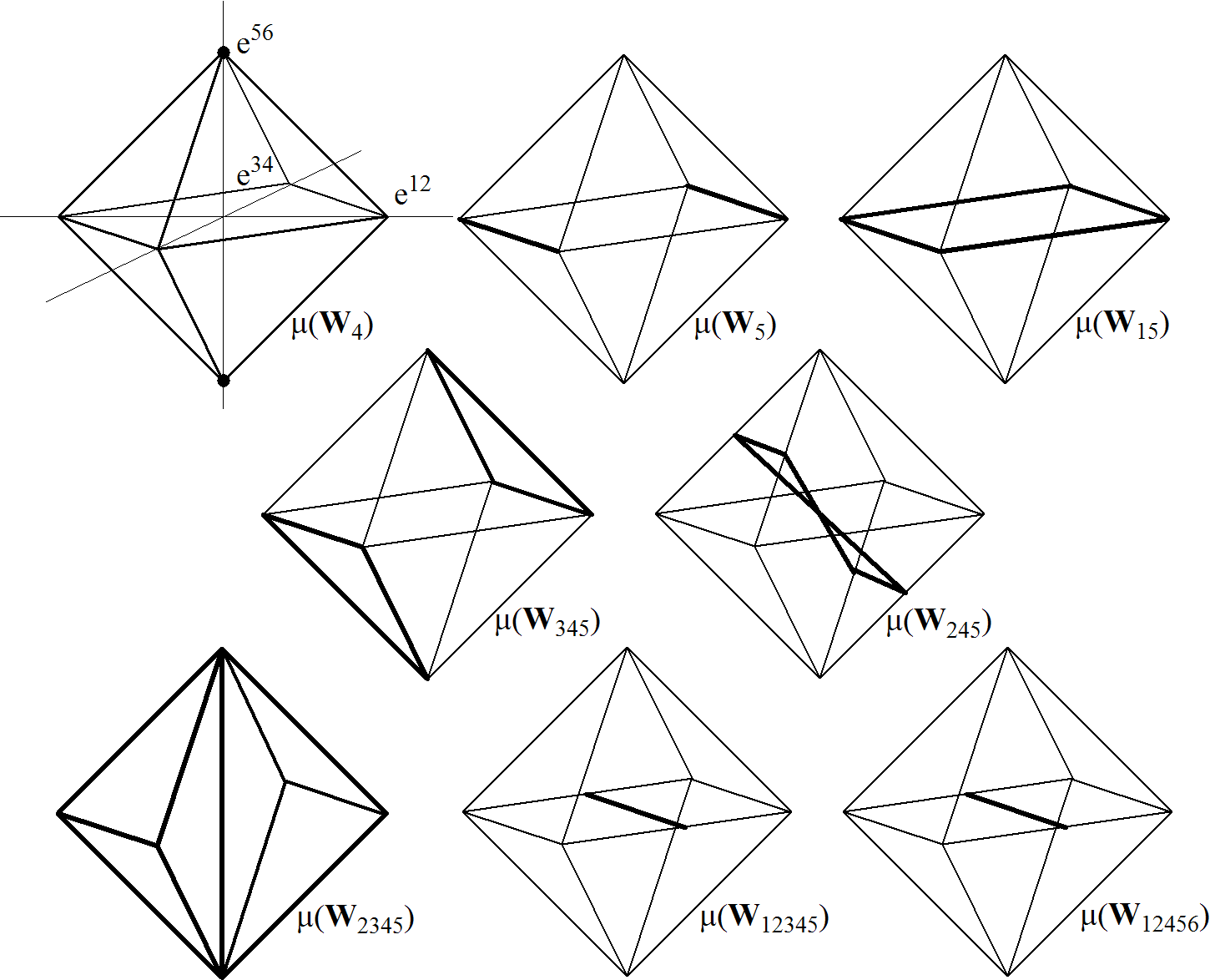
Figure 1: Images by $\mu_{T}$ of the ITV’s of OPS’S in the moment polytope of $\mathbb{G}\mathrm{r}_{2}(\mathbb{R}^{6})$.

Proof. The images of each ITV are obtained by elementary computations taking the projection on $\langle e^{12},e^{34},e^{56}\rangle$ of the simple $2$-form $v^{1}\wedge v^{2}$ associated to the OPS. In particular the points of $\mathbf{W}_{4}$ are fixed by the action of $\bar{T}$, $\mathbf{W}_{5}$, $\mathbf{W}_{15}$ and $\mathbf{W}_{345}$ are toric varieties, and as such can be represented as (well known) $\bar{T}$-orbit fibrations over their images by $\mu_{T}$. As $\mathbf{W}_{245}$ and $\mathbf{W}_{2345}$ are $\bar{T}$-stable and their intrinsic quotient is determined just by a dimensional check.

The sets $\mathbf{W}_{12345}$ $\mathbf{W}_{12456}$ are not $\bar{T}$-stable, but as $J_{2}$ and $J_{3}$ commute with the restriction $\bar{T}^{2}$ of $\bar{T}$ to $\mathscr{K}$, equation (28) is $\bar{T}^{2}$-invariant. The $\bar{T}^{2}$-orbit of the unit form $f=\sum_{1}^{4}x_{i}e^{i}$ depends on the value of $x_{1}^{2}+x_{2}^{2}$ in $[0,1]$. The generic $\bar{T}^{2}$-orbit in the base space of the fibration ($S^{3}$) is a two-torus. Values 0 and 1 correspond to degenerate $S^{1}$ orbits in $\langle e^{3},e^{4}\rangle$ and $\langle e^{1},e^{2}\rangle$. The $\bar{T}^{2}$-orbits of $Y_{1}J_{2}\mathbf{f}+Y_{2}J_{3}\mathbf{f}\in\mathscr{K}$ are analogously described. The couple $(Y_{1},Y_{2})$ determines distinguished $\bar{T}^{2}$-orbits on the fibres but it is easy to see, via standard parametrization of the $\bar{T}^{2}$-action on $\mathscr{K}$, that the orbit depends on $Y_{1}^{2}+Y_{2}^{2}\in(0,1)$. The set of orbits is parametrized by $[0,1]\times(0,1)$. Both $\mathbf{W}_{12345}$ and $\mathbf{W}_{12456}$ project on $\langle e^{12},e^{34}\rangle$ onto the line:

$$X=Y_{1}(x_{1}x_{4}+x_{2}x_{3})+Y_{2}(x_{2}x_{4}-x_{1}x_{3})=-Y.$$ (31)

The projection imposes a one-dimensional constrain, so the set of orbits in the inverse image of each point of $\mu_{T}(\mathbf{W}_{12345})$ and $\mu_{T}(\mathbf{W}_{12456})$ is one-dimensional.∎

For a more precise description of the intrinsic quotient of $\mathbf{W}_{12345}$ and $\mathbf{W}_{12456}$, an explicit parametrization of the symplectic quotient of $\mathbb{G}\mathrm{r}_{2}(\mathbb{R}^{6})$ is needed.

Remark 16.

The inclusions of ITV’s are very well represented by the moment polytopes. The compactification described in Remark 9 can be also visualized, $\mu_{T}(\mathbf{T}_{11})$ is the origin, $\mu_{T}(\mathbf{T}_{01})$ is the vertical segment connecting $\pm e^{56}$ etc.

The author believes that the rich geometry, which emerges in the analysed case, will stimulate the construction of a general theory on Intrinsic Torsion Varieties.

References

$[1]$ E. Abbena, S. Garbiero, and S. Salamon. Almost Hermitian geometry of 6-dimensional nilmanifolds. Ann. Sc. Norm. Sup., $30,\kern 2.0pt147-170,2001$.

$[2]$ D. E. Blair. Geometry of manifolds with structural group $U(n)\times O(s)$. Journal of differential geometry, $4,\kern 2.0pt155-167,\kern 2.0pt1970$.

$[3]$ R. Bryant. Calibrated embeddings in the special lagrangian and coassociative cases. Ann. Global Anal. Geom. – Special issue in memory of Alfred Gray (1939-1998), $18$, no. $3-4,\kern 2.0pt405-435,\kern 2.0pt2000$.

$[4]$ F. M. Cabrera and A. Swann. The intrinsic trosion of almost quaternion-hermitian manifolds. Syddansk Universitet, Preprint No.6 ISSN No. $0903-3920$, July $2007$.

$[5]$ S. Chiossi and A. Swann. $G_{2}$ -structures with torsion from half-integrable nilmanifolds. Journal of Geometry and Physics, $54,\kern 2.0pt265-285,\kern 2.0pt2005$.

$[6]$ D. Conti-A.Tomassini. Special symplectic six-manifolds. Quart J. Math, $58,\kern 2.0pt297-311,\kern 2.0pt2007$.

$[7]$ A. Gray and L. Hervella. The sixteen classes of almost Hermitian manifolds and their linear invariants. Ann. Mat. Pura Appl., $123,\kern 2.0pt35-58,\kern 2.0pt1980$.

$[8]$ G. Mihaylov. Special Riemannian structures in six dimensions. Doctoral thesis, University of Milan, $2008$.

$[9]$ G. Mihaylov. Toric moment mappings and Riemannian structures. Geometriae Dedicata, ISSN $0046-5755$, DOI $10.1007/s10711-012-9720-6,2012$.

$[10]$ G. Mihaylov and S. Salamon. Intrinsic torsion varieries. Note di matematica Universitá di Lecce, Suppl. N. $1,\kern 2.0pt349-376.,\kern 2.0pt2009$.

$[11]$ A. M. Naveira. A classification of Riemannian almost-product manifolds. Rendiconti di Matematica Roma, $3,\kern 2.0pt577-592,1983$.

$[12]$ S. Salamon. A tour of exceptional geometry. Milan J. Math., $59-94,\kern 2.0pt311-333,\kern 2.0pt2003$.

$[13]$ S. Sternberg. Lectures on Differential Geometry. New York Chelsea Publishing Company, $1983$.

$[14]$ K. Yano. On a structure defined by a tensor field f of type $(1,1)$ satisfying $f^{3}+f=0$. Tensor, $14,\kern 2.0pt99-109,\kern 2.0pt1963$.