Determining all gas properties in galaxy clusters from the dark matter distribution alone

Abstract

We demonstrate that all properties of the hot X-ray emitting gas in galaxy clusters are completely determined by the underlying dark matter (DM) structure. Apart from the standard conditions of spherical symmetry and hydrostatic equilibrium for the gas, our proof is based on the Jeans equation for the DM and two simple relations which have recently emerged from numerical simulations: the equality of the gas and DM temperatures, and the almost linear relation between the DM velocity anisotropy profile and its density slope. For DM distributions described by the NFW or the Sersic profiles, the resulting gas density profile, the gas-to-total-mass ratio profile, and the entropy profile are all in good agreement with X-ray observations. All these profiles are derived using zero free parameters. Our result allows us to predict the X-ray luminosity profile of a cluster in terms of its DM content alone. As a consequence, a new strategy becomes available to constrain the DM morphology in galaxy clusters from X-ray observations. Our results can also be used as a practical tool for creating initial conditions for realistic cosmological structures to be used in numerical simulations.

1 Introduction

Galaxy clusters are the largest equilibrated structures in the Universe, consisting mainly of dark matter (DM) and hot ionized gas in hydrostatic equilibrium in the overall potential well. Observations of this X-ray emitting gas allow for an accurate determination of the properties of the dominating DM structure, which can then be compared with the results of numerical N-body simulations.

More specifically, the strategy can be outlined as follows. In the first place, the equation of hydrostatic equilibrium can be used to infer the DM density profile from X-ray data (Fabricant et al., 1980). Application of this technique in conjunction with present-day observations (Voigt & Fabian, 2006; Pointecouteau et al., 2005) yields density profiles which are in excellent agreement with those emerging from numerical simulations of structure formation (Navarro et al., 1996; Moore et al., 1998; Diemand et al., 2004; Stadel et al., 2008; Navarro et al., 2008). Moreover, using a very simple connection between the gas and DM temperatures which has been confirmed by numerical simulations, the equation of hydrostatic equilibrium can be combined with the Jeans equation for the DM to derive both the DM radial velocity dispersion and the velocity anisotropy profile (Hansen & Piffaretti, 2007; Host et al., 2009). Again, the resulting profiles turn out to be in excellent agreement with numerical simulations (Cole & Lacey, 1996; Carlberg et al., 1997).

Measurements of the gas temperature profile have demonstrated its virtually universal properties (De Grandi & Molendi, 2002; Kaastra et al., 2004; Vikhlinin et al., 2005; Pointecouteau et al., 2005; Voigt & Fabian, 2006). This universality appears surprising since the temperature profile should encode information about the violent gravitational processes taking place during the cluster formation, as well as any additional energy input, e.g. from a central heat engine, and these processes are expected to differ significantly from structure to structure. The gas density profile also exhibits a roughly universal behaviour, which has allowed observers to fit remarkably simple forms, e.g. a beta-profile (Cavaliere & Fusco-Femiano, 1976; Sarazin, 1986), to the data.

A natural question arises as to whether the properties of the hot X-ray emitting gas in galaxy clusters can be predicted from first principles starting from the cluster DM distribution alone.

Attempts in that direction have been pioneered by (Makino et al., 1997; Suto et al., 1998). Our goal is to go a step further along this direction, relaying upon information on the internal cluster dynamics which has become available only quite recently.

More specifically, we will show how the gas density profile can be obtained directly from the underlying DM profile, by combining the equation of hydrostatic equilibrium for the gas and the Jeans equation for the DM under the standard assumption of spherical symmetry. Besides the above-mentioned relation between the gas and DM temperatures, our derivation rests upon a very simple connection between the DM velocity anisotropy and the slope of its density profile, which has recently emerged in numerical simulations (Hansen & Moore, 2006; Hansen & Stadel, 2006). We thereby demonstrate that the gas density profile is completely determined once the gravitationally dominant DM density profile is given. Since the gas temperature profile is also known, it turns out that the DM distribution dictates all the gas properties uniquely. Besides conceptually relevant in itself, this fact allows to predict the X-ray luminosity profile of a cluster in terms of its DM content alone by a method similar to the one put forward by Makino et al. (1997); Suto et al. (1998). So, a new strategy becomes available to constrain the DM morphology in galaxy clusters from X-ray observations. Moreover, our findings can be employed as a practical tool for creating initial conditions for realistic cosmological structures to be used in numerical simulations.

2 Background

We start by recalling some basic information which will be instrumental for our analysis. We restrict our attention throughout to regular clusters, which are supposed to be spherically symmetric and relaxed. The condition of hydrostatic equilibrium for the X-ray emitting gas can be written as

$$\frac{k_{B}T_{g}}{\mu m_{p}}\,\left(\frac{\mathrm{d}\ln\rho_{g}}{\mathrm{d}\ln r}+\frac{\mathrm{d}\ln T_{g}}{\mathrm{d}\ln r}\right)+\frac{GM_{\mathrm{tot}}(r)}{r}=0~{},$$ (1)

where $\rho_{g}(r)$ and $T_{g}(r)$ are the gas density and temperature profiles, respectively, $\mu\simeq 0.61$ is the mean molecular weight for the intracluster gas, $m_{p}$ is the proton mass and $M_{\mathrm{tot}}(r)$ represents the total mass inside radius $r$. Two conditions have to be satisfied in order for Eq. (1) to hold. First, it should be applied to a region considerably larger than the gas mean free path, so that local thermodynamic equilibrium is established. Second, the cooling time in that region should be larger than the age of the cluster, so that no bulk motion occurs. The latter condition is generally met outside the central region, where the presence of a cooling flow often requires Eq. (1) to be replaced by the Euler equation (with the velocity term playing a nonnegligible role). Because of collisional relaxation, the gas velocity distribution is isotropic and its temperature can be expressed in terms of the one-dimensional velocity dispersion ${\sigma_{g}^{2}}$ as

$$T_{g}=\frac{\mu m_{p}{\sigma}^{2}_{g}}{k_{B}}~{}.$$ (2)

Assuming complete spherical symmetry for the DM distribution, the two tangential components of the DM velocity dispersion, denoted by ${\sigma}_{t}^{2}$, are necessarily equal, but they are generally allowed to differ from the radial component ${\sigma}_{r}^{2}$, since DM is supposed to be collisionless. It is usual to quantify the DM velocity anisotropy by

$$\beta\equiv 1-\frac{{\sigma}^{2}_{t}}{{\sigma}^{2}_{r}}$$ (3)

and we find it convenient to introduce the mean DM one-dimensional velocity dispersion $\sigma_{\mathrm{DM}}^{2}$ as

$$\sigma^{2}_{\mathrm{DM}}\equiv\frac{1}{3}\left({\sigma}^{2}_{r}+2{\sigma}^{2}_{t}\right)=\left(1-\frac{2}{3}\beta\right){\sigma}^{2}_{r}~{}.$$ (4)

Moreover, in analogy with the case of a gas, we also define the DM temperature as Hansen & Piffaretti (2007)

$$T_{\mathrm{DM}}\equiv\frac{\mu m_{p}{\sigma^{2}_{\mathrm{DM}}}}{k_{B}}=\frac{\mu m_{p}}{k_{B}}\left(1-\frac{2}{3}\beta\right){\sigma}^{2}_{r}~{}.$$ (5)

Of course, the collisionless nature of DM prevents any definition of temperature in the thermodynamic sense and in fact $T_{\mathrm{DM}}$ is simply meant to quantify the average velocity dispersion over the three spatial directions. Any completely spherically symmetric and relaxed DM configuration obeys the Jeans equation

$$\sigma^{2}_{r}\,\left(\frac{\mathrm{d}\ln\rho_{\mathrm{DM}}}{\mathrm{d}\ln r}+\frac{\mathrm{d}\ln\sigma^{2}_{r}}{\mathrm{d}\ln r}+2\beta\right)+\frac{GM_{\mathrm{tot}}(r)}{r}=0~{},$$ (6)

where $\rho_{\mathrm{DM}}(r)$ denotes the DM density profile (Binney & Tremaine, 1987).

3 The temperature profile

Early studies of the X-ray emission from regular clusters were based on the assumption of an isothermal gas distribution, simply because the Einstein observatory and ROSAT were unable to determine the cluster temperature profiles. The observed X-ray emission is produced by thermal bremsstrahlung (Sarazin, 1986), so for $T_{g}=\mathrm{const.}$ it follows that $\rho_{g}(r)$ is proportional to the square root of the deprojected X-ray surface brightness. In such a situation, a good fit to the data was provided by the beta-model (Cavaliere & Fusco-Femiano, 1976; Sarazin, 1986)

$$\rho_{g}(r)=\frac{\rho_{g}(0)}{\left[1+\left(\frac{r}{a_{X}}\right)^{2}\right]^{3{\beta_{\mathrm{fit}}}/2}}~{},$$ (7)

where $a_{X}<0.5\,{\mathrm{Mpc}}$ is the X-ray core radius. Note that $\beta_{\mathrm{fit}}$ has nothing to do with the DM velocity anisotropy. Typically, most of the emission comes from the region $r>0.5\,{\mathrm{Mpc}}$, and so Eq. (7) can be approximated by the power-law

$$\rho_{g}(r)\simeq\rho_{g}(0)\left(\frac{r}{a_{X}}\right)^{-3{\beta_{{\mathrm{fit}}}}}~{}.$$ (8)

Now, by inserting Eq. (8) and $T_{g}=\mathrm{const}.$ into Eq. (1), we find

$$M_{\mathrm{tot}}(r)=\left(\frac{3{\beta}_{\mathrm{fit}}{\sigma}^{2}_{g}}{G}\right)r~{},$$ (9)

where Eq. (2) has been used. As is well known, under the assumption of isotropic velocity distribution ($\beta=0$), a mass profile of the form $M(r)\propto r$ describes a singular isothermal sphere (SIS) model in which the velocity dispersion is everywhere constant (Binney & Tremaine, 1987). Denoting by $\sigma$ the one-dimensional velocity dispersion, we explicitly have $M(r)=\left(2\sigma^{2}/G\right)r$. Owing to the fact that the leading contribution to $M_{\mathrm{tot}}(r)$ comes from DM, it follows that $M_{\mathrm{tot}}(r)\simeq M_{\mathrm{DM}}(r)$. As a consequence, Eq. (9) can be rewritten as

$$M_{\mathrm{DM}}(r)\simeq\left(\frac{2{\sigma^{2}_{\mathrm{DM}}}}{G}\right)r$$ (10)

and the comparison of Eqs. (9) and (10) entails in turn

$${\sigma^{2}_{\mathrm{DM}}}\simeq 1.5\,{\beta}_{\mathrm{fit}}\,{\sigma}^{2}_{g}~{}.$$ (11)

Observations performed with the Einstein observatory and ROSAT yield $0.5<{\beta}_{\mathrm{fit}}<0.9$ with a median ${\beta}_{\mathrm{fit}}\simeq 0.67$ (Bahcall & Lubin, 1994). Thus, on average we get

$${\sigma^{2}_{\mathrm{DM}}}\simeq{\sigma}^{2}_{g}~{},$$ (12)

which implies

$$T_{\mathrm{DM}}\simeq T_{g}~{},$$ (13)

thanks to Eqs. (2) and (5).

Only with the advent of the ASCA and Beppo-SAX satellites did it become possible to measure the cluster temperature profiles, which turned out to be described by a polytropic gas distribution to first approximation. Higher-quality data are currently provided by Chandra and XMM-Newton satellites, which have shown that the gas temperature profiles possess a very simple and nearly universal behaviour (see Vikhlinin et al. (2006) for a thorough discussion). Basically, it increases rapidly from a small (possibly non-zero) value in the centre, to a maximum at a radius about $0.1\,r_{180}$, and then declines slowly by a factor of $2-3$ at $(0.6-0.8)\,r_{180}$. Here, $r_{180}$ is defined as the radius within which the mean total density is 180 times the critical density at the redshift of the cluster. The necessary X-ray background subtraction makes it very difficult to accurately measure the temperature further out.

As mentioned above, our main goal is the determination of the gas density profile ${\rho}_{g}(r)$ once a specific dark matter distribution $M_{\mathrm{DM}}(r)$ is given. Supposing as before that $M_{\mathrm{tot}}(r)\simeq M_{\mathrm{DM}}(r)$, it is evident that ${\rho}_{g}(r)$ follows from Eq. (1) provided that ${T}_{g}(r)$ is specified. Previous studies (Makino et al., 1997; Suto et al., 1998) accomplished this task by assuming

$${T}_{g}(r)\simeq\frac{G\mu m_{p}M_{\mathrm{DM}}(r)}{3k_{B}r}~{},$$ (14)

which was suggested to formalize the condition that the gas temperature is close to the virial temperature of the DM. However, the virial theorem is a global relation that characterizes a cluster as a whole – it just arises by integrating the Jeans equation over the system – and so its validity is open to criticism. Of course, in the lack of any other information about the gas temperature this was the only viable possibility. However, recent progress allows for a considerable improvement on this point.

As a matter of fact, this stumbling block can be side-stepped in a remarkably simple fashion. Because of the equivalence principle, the velocity of a test particle in an external gravitational field is independent of the particle mass. This circumstance leads to the guess

$$T_{\mathrm{DM}}(r)=\kappa\,T_{g}(r)~{}.$$ (15)

This relation was tested against numerical simulations (Host et al., 2009), which demonstrated its validity with $\kappa=1$ to a very good approximation. These numerical simulations (Kay et al., 2007; Springel, 2005; Valdarnini, 2006) are reliable only on scales greater than $\sim 0.1\,r_{2500}$, while the best X-ray observations are sensitive to a radius which is almost a factor 3 smaller. It is therefore possible that heating or cooling may shift $\kappa$ away from unity in the very centre. Hence, outside that region $\kappa=1$ is expected. Actually, a look back at Eq. (13) confirms the remarkable fact that $\kappa=1$ holds regardless of the actual shape of the DM velocity anisotropy profile $\beta(r)$. As we shall see, starting from a specific underlying DM density profile $\rho_{\mathrm{DM}}(r)$, one can evaluate $T_{\mathrm{DM}}(r)$ and then get the gas temperature profile $T_{g}(r)$ uniquely.

Before closing this section, a remark is in order. Observations show that some clusters lack a central cooling flow. In such a situation, hydrostatic equilibrium is expected to hold all the way down to the centre. Actually, for typical central values of the electron number density $n_{e}\simeq 1{\mathrm{cm}}^{-3}$ and temperature $T\simeq 10^{8}\,{\mathrm{K}}\simeq 8.5\,{\mathrm{keV}}$ (Sarazin, 1986), the scattering time turns out to be $t_{\mathrm{scat}}\sim 10^{2}\mathrm{yr}$, which is much smaller than the corresponding gas cooling time $t_{\mathrm{cool}}\sim 10^{7}\mathrm{yr}$, so that local hydrostatic equilibrium is indeed fulfilled outside a central spherical region of radius $\sim 1\,{\rm pc}$. Assuming further that the gas temperature is roughly constant in the inner cluster region, the gas density profile cannot be cuspy as long as $M_{\mathrm{DM}}(r)\propto r^{a}$ with $a>1$ for $r\to 0$. This is at odds with blind extrapolations of fitting formulae for the temperature and density such as those used in Vikhlinin et al. (2006).

4 The density profile

We now proceed to the actual derivation of the gas density profile ${\rho_{g}}(r)$ from the properties of the dominating DM distribution.

As a preliminary step, we notice that Eqs. (1) and (6) can be trivially combined to yield

$$\frac{k_{B}T_{g}}{\mu m_{p}}\,\left(\frac{\mathrm{d}\ln\rho_{g}}{\mathrm{d}\ln r}+\frac{\mathrm{d}\ln T_{g}}{\mathrm{d}\ln r}\right)$$

$$=\sigma^{2}_{r}\,\left(\frac{\mathrm{d}\ln\rho_{\mathrm{DM}}}{\mathrm{d}\ln r}+\frac{\mathrm{d}\ln\sigma^{2}_{r}}{\mathrm{d}\ln r}+2\beta\right)\,.$$ (16)

Owing to Eqs. (5) and (15) with $\kappa=1$, straightforward manipulations permit to recast Eq. (4) into the form

$$\gamma_{g}=\frac{1}{1-\frac{2}{3}\beta}\left(\gamma_{\mathrm{DM}}+2\beta+\textstyle\frac{2}{3}\displaystyle\beta\frac{\mathrm{d}\ln\sigma^{2}_{r}}{\mathrm{d}\ln r}+\frac{2}{3}\frac{\mathrm{d}\beta}{\mathrm{d}\ln r}\right)~{},$$ (17)

where we have defined the density slopes $\gamma_{\mathrm{DM}}(r)$ of the DM and $\gamma_{g}(r)$ of the gas as

$$\gamma_{X}(r)\equiv\frac{\mathrm{d}\ln{\rho}_{X}}{\mathrm{d}\ln r}~{},$$ (18)

with $X$ standing for either $\mathrm{DM}$ or $g$. We stress that Eq. (17) captures a crucial point of the present investigation: only the gas density slope appears on its left-hand side, whereas only quantities pertaining to the DM appear on its right-hand side. It should be appreciated that this result merely relies upon the equality of gas and DM temperatures and – unlike in previous studies (Cavaliere & Fusco-Femiano, 1976; Makino et al., 1997; Suto et al., 1998) – no assumption is being made about the actual gas temperature structure (e.g. isothermal or polytropic).

Next, we use the fact that the DM anisotropy profile ${\beta}(r)$ turns out to be almost linearly related to the slope of the DM density profile $\gamma_{\mathrm{DM}}(r)$. This result has been obtained from numerical simulations and holds with a scatter of about 0.05 (Hansen & Moore, 2006; Hansen & Stadel, 2006). It has recently been confirmed by high-resolution numerical simulations (Navarro et al., 2008) and moreover it has been derived analytically (Hansen, 2008) (see also Zait et al. (2008); Wojtak et al. (2008); Salvador-Solé et al. (2007)).

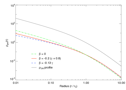
Figure 1: The derived gas density profile, assuming that $\rho_{g}/\rho_{\mathrm{DM}}=10\%$ at $r_{0}$, which is the scale length of the NFW profile. The upper curve (black) is the DM density, and the 3 lower lines show gas profiles modelled with extreme variations in the possible DM velocity anisotropy (green dot-dashed is isotropic ($\beta=0$), red solid is using $\beta=-\,0.2\,(\gamma+0.8)$ (Hansen & Stadel, 2006), and blue dashed is using $\beta=-\,0.13\,\gamma$ (Hansen, 2008)).

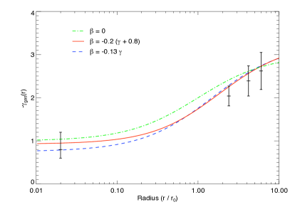
Figure 2: The derived slope of the gas density profile, assuming an NFW profile for the DM. Same notation as in Figure 1. The inner point is taken from Vikhlinin et al. (2006) and the three outer points are taken from Ettori & Balestra (2008).

Getting the gas density profile ${\rho}_{g}(r)$ now involves a few simple steps. Our only input is the DM density profile ${\rho}_{\mathrm{DM}}(r)$, like e.g. an NFW profile. Thanks to Eq. (18), we rewrite the Jeans equation (6) as

$$r\frac{\mathrm{d}\sigma^{2}_{r}}{\mathrm{d}r}+\sigma^{2}_{r}\,\Bigl{(}{\gamma}_{\mathrm{DM}}(r)+2{\beta}(r)\Bigr{)}+\frac{GM_{\mathrm{tot}}(r)}{r}=0~{},$$ (19)

whose solution is easily found to be

$$\sigma^{2}_{r}(r)=\frac{G}{B(r)}\int_{r}^{\infty}{\mathrm{d}}r^{\prime}\,\frac{B(r^{\prime})\,M_{\mathrm{tot}}(r^{\prime})}{{r^{\prime}}^{2}}~{},$$ (20)

with

$$B(r)\equiv\rho_{\mathrm{DM}}(r)\,\mathrm{exp}\left\{-\,2\int_{r}^{\infty}\mathrm{d}r^{\prime}\,\frac{\beta(r^{\prime})}{r^{\prime}}\right\}.$$ (21)

Using the relation between $\beta(r)$ and $\gamma_{\mathrm{DM}}(r)$, we finally obtain the gas density profile from Eqs. (17) and (18).

In practice, such a procedure can be implemented iteratively. In first approximation, we assume that the gas mass contribution is negligible, so that we have $M_{\mathrm{tot}}(r)=M_{\mathrm{DM}}(r)$. In the next iterations, we include the gas mass in the calculation of $\sigma_{r}^{2}(r)$. Although the gas mass is taken into account perturbatively, any desired accuracy can be achieved by a sufficient number of iterations.

An example of the application of this strategy is shown in Figure 1, where the DM density is assumed to follow an NFW profile (black solid line). The three lower lines are the gas density profiles obtained with a range of different possible DM velocity anisotropy profiles. The details of the gas density profile are easier seen in the slope, which is shown in Figure 2. Note that for an inner DM slope of about $1$ (in agreement with the observations (Voigt & Fabian, 2006; Pointecouteau et al., 2005)) the inner gas slope should also be close to $1$. This is in good agreement with the fits from Vikhlinin et al. (2006), which have an average of $0.8$ for the extrapolated inner slope. Also the slopes found by Ettori & Balestra (2008) agrees with an NFW profile.

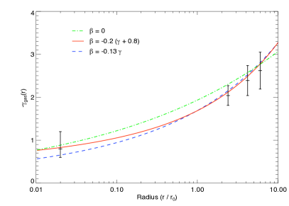
Figure 3: The slope of the gas density profile, assuming a Sersic profile with $n=5$ for the DM. Same notation as in Figures 1 and 2.

A widely used alternative to the NFW profile is the Sersic (or Einasto) profile, which generalizes the de Vaucouleurs profile traditionally used to fit the optical surface brightness of elliptical galaxies. It has been shown that the Sersic profile models the deprojected DM density at least as well as the NFW (Navarro et al., 2004; Merritt et al., 2006; Salvador-Solé et al., 2007). This profile contains 3 free parameters: two scaling constants for the density and the radius – $\rho_{0}$ and $r_{0}$ respectively – and one shape parameter $n$

$$\rho(r)=\rho_{0}\exp\left[-\,b_{n}\left(\left(\frac{r}{r_{0}}\right)^{\frac{1}{n}}-1\right)\right]~{}.$$ (22)

The constant $b_{n}$ is a function of the index $n$ and is tabulated e.g. by Mazure & Capelato (2002). The radial velocity dispersion $\sigma_{r}$ derived from the Sersic profile has, like the NFW profile, the property of reaching its maximum near $r_{0}$ where the slope is $\gamma=2$. In Figure 3 we present the gas density slope, assuming a Sersic profile for the underlying DM density. There is not sufficient statistical power in the data to discriminate between the underlying DM density and/or velocity anisotropy profiles from this analysis.

Both the NFW and the Sersic profile are consistent with observations because they have the appropriate slope in the inner and outer observed region. Since we cannot exclude one or the other by relying upon their shape, we choose the NFW model for the underlying DM in the rest of our treatment.

Since the gas density profile differs from the underlying DM density profile, there will also be a radial variation in the local and cumulative gas fractions, which are defined as

$$\phi_{g}(r)=\frac{\rho_{g}(r)}{\rho_{\mathrm{tot}}(r)}$$ (23)

and

$$f_{g}(r)=\frac{M_{g}(r)}{M_{\mathrm{tot}}(r)}~{},$$ (24)

respectively. In order to test this in more detail, we used the 16 clusters analysed in Host et al. (2009), which is a selection of highly relaxed clusters at both low and intermediate redshifts (Kaastra et al., 2004; Piffaretti et al., 2005; Morandi et al., 2007) observed with XMM-Newton and Chandra. Under the assumption of hydrostatic equilibrium, we find the local gas fraction exhibited in Figure 4. The local gas fraction clearly increases as a function of radius, which demonstrates that the DM velocity anisotropy cannot vanish (green dot-dashed line in Figure 4). The gas density fraction roughly increases as a power-law in radius and we have approximately $f_{g}(r)\sim r^{0.5}$. The solid (red) and dashed (blue) lines are for NFW DM profiles, with different radial DM velocity anisotropies. From Figure 4 there is a clear difference between the data and the predictions in the outer region, which may be due to an underestimation of the total mass due to breakdown of hydrostatic equilibrium (Piffaretti & Valdarnini, 2008).

It is important to keep in mind that these profiles do not contain any free parameters. Every quantity is calculated from the dark matter distribution alone.

The agreement in the inner region is better and it should be kept in mind that different DM density and velocity anisotropy profiles give rise to different curves. It may therefore be possible to use the shape of $\phi_{g}(r)$ to recover these DM profiles in the future.

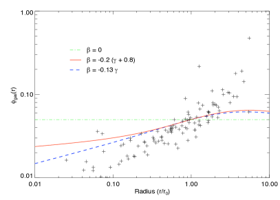
Figure 4: The observed $\phi_{g}$ from 16 relaxed galaxy clusters. We have scaled the gas mass fraction with free parameters, to make the radial variation more visible. There is a rough trend that the gas mass fraction increases as $r^{0.5}$, which is in clear disagreement with the assumption that the DM velocity anisotropy should vanish. The 3 curves all assume an NFW density profile, and different assumed connections between the DM slope and velocity anisotropy, as in Figure 1.

As a further step, we discuss some of the implications of our main result. Indeed, with a full description of the gas that is directly derived from the dark matter distribution, we can predict additional observable quantities besides the gas fraction described above.

One of these quantities is the entropy, which is often characterized by the adiabatic coefficient $K_{g}$ of the gas

$$K_{g}=\frac{k_{B}T}{\mu m_{p}}\rho^{-2/3}=\sigma^{2}_{g}\,\rho^{-2/3}~{}.$$ (25)

Our previous results entail that these profiles are almost perfect power laws regardless of the $\beta$ profile. The slope changes slightly for the different $\beta$ profiles (between 1.1 and 1.3). This theoretical prediction is in good agreement with the X-ray observations, which generally produce power-law entropy profiles (Piffaretti et al., 2005; Pratt, G. W. & Arnaud, M., 2005; Donahue et al., 2006).

Another quantity that we are able to predict is the gas X-ray emissivity $\epsilon$. As a matter of fact, $\epsilon$ can be estimated either analytically – because $\epsilon\propto n^{2}T^{\frac{1}{2}}$ – or by numerical codes like MeKaL (Mewe et al., 1985) in order to include the line emission contribution. The latter strategy is especially well suited for cooler clusters, because a substantial amount of their luminosity stems from emission lines. On the other hand, the luminosity of hotter clusters is dominated by the continuum emission. In either case, the surface brightness can be inferred from a given DM profile and this can in turn be compared with observations. In this way, it is possible to construct an algorithm that adjusts the proposed DM profile until the surface brightness best-fits observations and thereby single out the optimal DM profile. It is clear that this method will be limited due to clumpiness, which may be crucial in the outer parts, and one may have to combine the X-ray analysis with SZ observations to correctly extract all the profiles. We hope to discuss these aspects in more detail in the future.

Whereas numerical simulations have demonstrated that the gas and dark matter temperatures are equal in large parts of a galaxy cluster, they cannot probe the very centre of the clusters. It is therefore possible that $\kappa$ in Eq. (15) departs from unity as $r\to 0$ if there is significant cooling or heating. However, in our derivation of the gas density profile we have assumed $\kappa=1$ everywhere.

It goes without saying that we can turn the argument around and use the observed gas profile to determine $\kappa$. Basically, we can insert Eq. (15) into Eq. (4) and solve for $\kappa$. Furthermore, since we are now interested in the central region where $\beta$ is likely to be vanishingly small, we discard all terms involving $\beta$ in the resulting equation. So, in place of Eq. (17) we presently get

$$\kappa=\frac{\gamma_{g}+{\mathrm{d}}\ln\sigma^{2}_{r}/{\mathrm{d}}\ln r}{\gamma_{\mathrm{DM}}+{\mathrm{d}}\ln\sigma^{2}_{r}/{\mathrm{d}}\ln r}~{},$$ (26)

which in principle allows to measure $\kappa$ directly from X-ray observations. Such measurement can be used or tested in future numerical simulations when the increased particle number will allow simulations to probe closer to the cluster centre.

5 Conclusions

We have shown that all properties of the hot X-ray emitting gas in galaxy clusters are completely determined by its underlying DM structure. Apart from the standard conditions of spherical symmetry and hydrostatic equilibrium for the gas, our proof is based on the Jeans equation for the DM and two simple relations which have recently emerged from numerical simulations. One is the equality of the gas and DM temperatures. The other is an almost linear relationship between the DM velocity anisotropy profile and its density slope. For DM distributions described by the NFW or the Sersic profiles, the resulting gas density profile, the gas-to-total-mass ratio profile and the entropy profile are all in good agreement with X-ray observations. We feel that our result is conceptually relevant in itself. Moreover, it allows to predict the X-ray luminosity profile of a cluster in terms of its DM content alone. Therefore, a new strategy becomes available to constrain the DM morphology in galaxy clusters from X-ray observations (Frederiksen et al., 2009). This strategy may constrain morphology parameters better because of the tighter errors on surface brightness, but requires the structure to be very relaxed, and ignores clumpiness, and thus cannot be used on every cluster. Our results can also be used as a practical tool for creating initial conditions for realistic cosmological structures to be used in numerical simulations.

References

- Allen et al. (2004) Allen, S. W., Schmidt, R. W., Ebeling, H., Fabian, A. C., & van Speybroeck, L. 2004, MNRAS, 353, 457
- Bahcall & Lubin (1994) Bahcall, N. A., & Lubin L. M. 1994, ApJ, 426, 513
- Binney & Tremaine (1987) Binney, J., & Tremaine, S. 1987, Princeton, NJ, Princeton University Press, 1987.
- Carlberg et al. (1997) Carlberg, R. G., et al. 1997, ApJ, 485, L13
- Cavaliere & Fusco-Femiano (1976) Cavaliere, A., & Fusco-Femiano, R. 1976, A&A, 49, 137
- Cole & Lacey (1996) Cole, S., & Lacey, C. 1996, MNRAS, 281, 716
- De Grandi & Molendi (2002) De Grandi, S., & Molendi, S. 2002, ApJ, 567, 163
- Diemand et al. (2004) Diemand, J., Moore, B., & Stadel, J. 2004, MNRAS, 353, 624
- Donahue et al. (2006) Donahue, M., Horner, D. J., Cavagnolo, K. W., & Voit, G. M. 2006, ApJ, 643, 730
- Ettori & Balestra (2008) Ettori, S. & Balestra, I. ArXiv e-prints, 2008, arXiv:0811.3556 [astro-ph].
- Fabricant et al. (1980) Fabricant, D, Lecar, M. & Gorenstein, P. 1980, ApJ241, 552
- Frederiksen et al. (2009) Frederiksen et al. 2009, in preparation
- Merritt et al. (2006) Merritt, D., Graham, A. W., Moore, B., Diemand, J., & Terzić, B. 2006, AJ, 132, 2685
- Hansen & Moore (2006) Hansen S. H., & Moore B 2006, New Astron., 11, 333
- Hansen & Stadel (2006) Hansen, S. H., & Stadel, J. 2006, Journal of Cosmology and Astro-Particle Physics, 5, 14
- Hansen & Piffaretti (2007) Hansen, S. H., & Piffaretti, R. 2007, A&A, 476, L37
- Hansen (2008) Hansen, S. H. 2008, arXiv:0812.1048
- Host et al. (2009) Host, O., Hansen, S. H., Piffaretti, R., Morandi, A., Ettori, S., Kay, S. T., & Valdarnini, R. 2009, Astrophys. J. 690, 358
- Kaastra et al. (2004) Kaastra, J. S., et al. 2004, A&A, 413, 415
- Kay et al. (2007) Kay, S. T., da Silva, A. C., Aghanim, N., Blanchard, A., Liddle, A. R., Puget, J.-L., Sadat, R., & Thomas, P. A. 2007, MNRAS, 377, 317
- Makino et al. (1997) Makino, N., Sasaki, S. & Suto, Y. 1998, ApJ, 497, 555
- Mazure & Capelato (2002) Mazure, A. & Capelato, H. V. A&A, 2002, 383, 384-389
- Mewe et al. (1985) Mewe, R.; Gronenschild, E. H. B. M. & van den Oord, G. H. J. A&AS, 1985, 62, 197-254
- Moore et al. (1998) Moore, B., Governato, F., Quinn, T., Stadel, J. & Lake G. 1998, ApJ, 499, 5
- Morandi et al. (2007) Morandi, A., Ettori, S., & Moscardini, L. 2007, MNRAS, 379, 518
- Navarro et al. (1996) Navarro, J. F., Frenk, C. S., & White, S. D. M. 1996, ApJ, 462, 563
- Navarro et al. (2004) Navarro, J. F., et al. 2004, MNRAS, 349, 1039
- Navarro et al. (2008) Navarro,J. F. et al. 2008, arXiv:0810.1522
- Piffaretti et al. (2005) Piffaretti, R., Jetzer, P., Kaastra, J. S. & Tamura, T. A&A, 2005, 433, 101-111
- Piffaretti & Valdarnini (2008) Piffaretti, R. & Valdarnini, R. 2008, arXiv:0808.1111
- Pratt, G. W. & Arnaud, M. (2005) Pratt, G. W. & Arnaud, M. A&A, 2005, 429, 791-806
- Pointecouteau et al. (2005) Pointecouteau, E., Arnaud, M., & Pratt, G. W. 2005, Astron. & Astrophys, 435, 1
- Salvador-Solé et al. (2007) Salvador-Solé, E., Manrique, A., González-Casado, G., & Hansen, S. H. 2007, ApJ, 666, 181
- Sarazin (1986) Sarazin, C. L. 1986, Reviews of Modern Physics, 58, 1
- Springel (2005) Springel, V. 2005, MNRAS, 364, 1105
- Stadel et al. (2008) Stadel, J. et al. 2008, arXiv:0808.2981
- Suto et al. (1998) Suto, Y., Sasaki, S., & Makino, N. 1998, ApJ, 509, 544
- Valdarnini (2006) Valdarnini, R. 2006, New Astron. 12, 71
- Vikhlinin et al. (2005) Vikhlinin, A., Markevitch, M., Murray, S. S., Jones, C., Forman, W., & Van Speybroeck, L. 2005, ApJ, 628, 655
- Vikhlinin et al. (2006) Vikhlinin, A., Kravtsov, A., Forman, W., Jones, C., Markevitch, M., Murray, S. S., & Van Speybroeck, L. 2006, Astrophys. J. 640, 691
- Voigt & Fabian (2006) Voigt, L. M., & Fabian, A. C. 2006, MNRAS, 368, 518
- Wojtak et al. (2008) Wojtak, R., Łokas, E. L., Mamon, G. A., Gottlöber, S., Klypin, A., & Hoffman, Y. 2008, MNRAS, 388, 815
- Zait et al. (2008) Zait, A., Hoffman, Y., & Shlosman, I. 2008, ApJ, 682, 835