Noisy continuous–opinion dynamics

Abstract

We study the Deffuant et al. model for continuous–opinion dynamics under the influence of noise. In the original version of this model, individuals meet in random pairwise encounters after which they compromise or not depending of a confidence parameter. Free will is introduced in the form of noisy perturbations: individuals are given the opportunity to change their opinion, with a given probability, to a randomly selected opinion inside the whole opinion space. We derive the master equation of this process. One of the main effects of noise is to induce an order-disorder transition. In the disordered state the opinion distribution tends to be uniform, while for the ordered state a set of well defined opinion groups are formed, although with some opinion spread inside them. Using a linear stability analysis we can derive approximate conditions for the transition between opinion groups and the disordered state. The master equation analysis is compared with direct Monte-Carlo simulations. We find that the master equation and the Monte-Carlo simulations do not always agree due to finite-size induced fluctuations that we analyze in some detail.

Keywords: Collective phenomena in economic and social systems: Interacting agent models. Non-equilibrium processes: Stochastic particle dynamics (Theory).

1 Introduction

The application of techniques and tools from nonlinear and statistical physics to understand the dynamics of opinion changes in a society has become a topic of interest in recent years [1]. A society can be thought of as a complex system composed by a large number of interacting individuals with diverse opinions. These opinions are not necessarily static, but they evolve due to a variety of internal as well as external factors, such as the influence of advertising and acquaintances, amongst others. As a result of this evolution, a consensus opinion could emerge (a vast majority on individuals adopting a similar opinion), or the population could fragment into a number of groups. To analyze the process of opinion formation, several models inspired from statistical mechanics have been developed. In those, the opinion held by an individual is a dynamical variable which evolves by some rules, usually with an important stochastic ingredient [2]. Models can be divided in two broad categories: discrete models where the opinion can only adopt a finite set of values [3, 4, 5], and continuous models where the opinion of an individual is expressed as a real number in a finite interval [6, 7, 8, 9]. Discrete models are useful when analyzing cases in which individuals are confronted with a limited number of options (a political election, for example) where one is forced to choose amongst a finite set of parties. Continuous models are more suitable to analyze cases in which a single issue (legalizing abortion, for example) is being considered and opinions can vary continuously from “completely against” to “in complete agreement”.

A continuous model introduced by Deffuant and collaborators [6] has received much attention recently. This model implements the bounded confidence mechanism by which two individuals only influence the opinion of each other if their respective opinions differ less than some given amount. In other words, people holding too distant opinions on an issue will simply ignore each other and will, hence, keep their original opinions. It is only through the interaction of not too distant people that we manage to modify our opinion. This model was in turn inspired by the Axelrod model for the dissemination of culture [10] and general threshold models [11] and has in turn inspired a large number of extensions and modifications [12, 13, 14, 15, 16, 17, 18, 19, 20].

In the Deffuant et al. model individuals meet in random pairwise encounters in a given connectivity network, but the subsequent evolution is completely deterministic. This leads to final states in which either perfect consensus has been reached or the population splits in a finite number of groups such that all individuals in one group have exactly the same opinion. We believe that such uniform states are not very realistic and some degree of discrepancy must appear within otherwise well defined groups. In this paper, we introduce an additional element of randomness in the dynamics. It aims to represent, certainly in a caricaturist manner, the element of free will present in all human decisions by which we do not follow blindly the opinion dictated by our relationships. Our aim is to analyze how the interplay between this free will and the interactions amongst individuals affects group formation in opinion dynamics. In the language of statistical mechanics, what we are doing is to add noise to the deterministic dynamics and analyze which aspects of the model are robust against the introduction of noise. Noise is introduced by allowing an individual opinion to change to another randomly chosen value in the whole opinion space. Under some circumstances this turns out to be equivalent to allowing each agent to return, at some random times, to a specific opinion preferred by him.

Our analysis, based upon numerical integrations of the corresponding master equation as well as Monte-Carlo simulations, reveals new and interesting phenomenology. There exists a critical value $m_{c}$ of the noise intensity, which depends on the confidence range, such that for noise larger than this value the system becomes disorganized and group formation does not occur. We provide a linear stability analysis that reproduces the order-disorder transition that occurs at $m_{c}$. For noise smaller than $m_{c}$, the steady-state probability distributions in opinion space broaden with respect to the noiseless case, but still have large peaks and group formation can be unambiguously defined by looking at the maxima of the distributions. The group formation occurs by a series of bifurcations that mimic those that occur in the noiseless case.

An important aspect of our work, that we want to stress here, is that the numerical Monte-Carlo simulations do not necessarily agree with the results of the master equation. This is due to the inherent finite-size-induced fluctuations that occur in the simulations. A similar warning is required when one tries to infer about possible applications of the model to real situations. For example, it is possible to find regions of bistability where dynamical transitions between a single group and two groups occur. These transitions do not occur in the infinite-size thermodynamic limit taken routinely in most studies. This stresses the role that a finite size has on the dynamics of social systems [25].

This paper is organized as follows. Deffuant et al. model is briefly reviewed in Sec. 2. The main results are presented in section 3, devoted to study this model in the presence of noise. In Sec. 4 we use a linear stability analysis to derive approximately the critical value of the noise intensity for the formation of opinion groups. Summary and conclusions are presented in Sec. 5.

2 Review of Deffuant et al. model

Let us consider a population with $N$ individuals. We will denote by $x_{n}^{i}$ the number representing the opinion on a given topic that individual $i$ has at time-step $n$. As mentioned in the introduction, the opinion is a real variable in a finite interval and, without loss of generality, we take $x_{n}^{i}\in[0,1]$. Initially, it is assumed that the values $x_{0}^{i}$ for $i=1,\dots,N$ are randomly distributed in the interval $[0,1]$. Dynamics is introduced to reflect that individuals interact, discuss, and modify their opinions. In the original version of the model [6], at time-step $n$ two individuals, say $i$ and $j$, are randomly chosen. If their opinions satisfy $|x_{n}^{i}-x_{n}^{j}|<\epsilon$, so that they are close enough, they are modified as:

$$\begin{array}[]{lcr}x_{n+1}^{i}&=&x_{n}^{i}+\mu(x_{n}^{j}-x_{n}^{i}),\cr x_{n+1}^{j}&=&x_{n}^{j}+\mu(x_{n}^{i}-x_{n}^{j}),\end{array}$$ (1)

otherwise they remain unchanged. Whether the opinions have been updated or not, time increases $n\to n+1$. As a consequence of the iteration of this dynamical rule, the system reaches a static final configuration which, depending on the values of the parameters $\epsilon$ and $\mu$, can be a state of full consensus where all individuals share the same opinion, or of fragmentation with several opinion groups. It is customary to introduce the time variable $t=n\Delta t$, where $\Delta t=1/N$, measuring the number of opinion updates per individual, or number of Monte-Carlo steps (MCS).

The parameter $\mu$ is restricted to the interval $(0,0.5]$. It determines the convergence time between individuals as well as the number of final groups [23, 24]. For small values of $\mu$, the individuals slightly change their opinions during meeting, while for $\mu=0.5$ the interacting individuals fully compromise and, after the meeting, they share the same opinion. As in most studies, we will adopt from now on in this paper the value $\mu=0.5$. The parameter $\epsilon$, which runs from $0$ to $1$, is the confidence parameter. Starting from uniformly distributed random values for the initial opinions, the typical realization is that for large values, $\epsilon\geq 0.5$, the system evolves to a state of consensus where all individuals share the same opinion and that, decreasing $\epsilon$, the population splits into opinion groups separated by distances larger than $\epsilon$.

The process can be described in terms of a master equation for the probability density function $P(x,t)$ for an individual opinion $x$ at time $t$. The Appendix contains a derivation of this master equation in the presence of the additional noise term described in section 3. Equation (8) with $m=0$ is the master equation for the noiseless original Deffuant et al. model, first obtained in [12]. A detailed analysis based on its numerical integration [12, 20] shows that there are four basic modes of group appearance, dominance, or splitting, which are called bifurcations [12, 20] in this context (see Fig. 1): nucleation of two minor groups symmetrically from the center of the opinion interval (type-1, such as the birth of two minor groups from the boundaries at $\epsilon=0.5$ in Fig. 1); nucleation of two major groups from the central one (type-2, as occurring at $\epsilon\approx 0.266$ in Fig. 1); nucleation of a minor central group (type-3, as occurring at $\epsilon\approx 0.222$ in the figure); and, finally, sudden increase of the mass of that central group accompanied by a sudden drift outwards in the location of the two major groups (type-4, at $\epsilon\approx 0.182$ in the figure). In this sequence “major” opinion groups contain a high fraction of the population, while “minor” groups contain a much smaller fraction (of the order of $10^{-2}$ or smaller). The bifurcation pattern repeats itself as $\epsilon$ decreases even further.

It is important to emphasize that the situation depicted in Fig. 1 is the result for steady solutions of the master equation attained at long times starting from a uniform initial distribution. Many other steady solutions of the master equation exist. In particular, any combination of delta-functions is a steady solution of the noiseless master equation provided they are separated by more than a distance $\epsilon$. We stress also that this analysis based upon the master equation corresponds to the limit case where the number of individuals $N$ tends to infinity. In Monte-Carlo simulations of the microscopic rules, or in practical applications with a necessarily finite number of individuals, some features need to be considered. It is still true that each realization ends up in a small number of groups (both of major and minor type), all individuals within a group holding exactly the same opinion. However, the exact location of the groups might vary with respect to the master equation prediction and minor groups might not appear depending on the particular realization and the total size of the population. Furthermore, there could be realizations in which even the number of observed major groups differs from the prediction of the master equation. These effects are more pronounced the smaller the number of individuals. In the same Fig. 1 we have plotted the distribution of observed groups, averaged over many realizations for two different number of individuals $N$, where the aforementioned properties can clearly be observed. For instance, for $\epsilon=0.28$, the master equation predicts that there should be only one major group, centered at $x=0.5$, and two minor groups. However, in almost half of the realizations with $N=1000$ individuals the opinions split instead in two major groups centered around $x=0.28$ and $x=0.72$ and, eventually, some minor extreme groups.

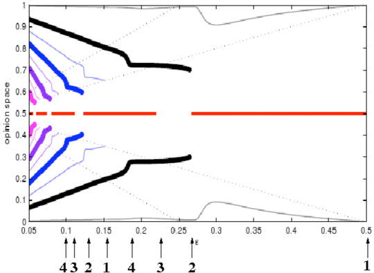
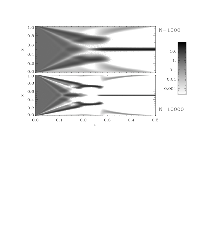
Figure 1: Top panel: bifurcation diagram of the noiseless Deffuant et al., model reproduced from reference [22], coming from a numerical analysis of the master equation of the model [12, 21]. Lines show the position of the opinion groups as a function of $\epsilon$. By arrows we indicate the location of the four basic types of bifurcations: type-1 at $\epsilon\approx 0.5$, type-2 at $\epsilon\approx 0.266$, type-3 at $\epsilon\approx 0.22$, type-4 at $\epsilon\approx 0.182$, and this pattern repeating as $\epsilon$ decreases even further [21]. In the bottom panels we plot in a logarithmic grey-scale the asymptotic probability distribution $P_{\infty}(x)$ (values smaller than $2\times 10^{-4}$ are plotted white), as a function of $\epsilon$, resulting from extensive numerical simulations of the microscopic model with $N=10^{3}$ and $N=10^{4}$ agents, respectively. Note that a single realization using the Monte-Carlo microscopic rules of the model leads to a probability distribution which is a sum of delta-functions. The distributions displayed in the panels are the result of an average over $10^{5}$ realizations for $N=10^{3}$ and $2\times 10^{4}$ realizations for $N=10^{4}$ and a histogram bin size $\Delta x=0.01$. In all cases, both in the master equation as in the Monte-Carlo simulations, the initial condition represents opinions which are random and uniformly distributed in the interval $[0,1]$.

3 Effect of noise

Noise is introduced as a random change of an individual’s opinion. Specifically, we modify the dynamics as follows: at time-step $n$ the original dynamical rule, Eq. (1), applies only with probability $1-m$. Otherwise, a randomly chosen individual $i$ changes his opinion to a new value $x_{n+1}^{i}$ drawn from a uniform distribution in the interval $[0,1]$ and all other opinions remain unchanged. The probability $m$ is a measure of the noise-intensity. Note that, quite generally, this rule is equivalent to allowing each agent to return to a specific, basal, opinion preferred by him, provided that the basal opinions are randomly distributed amongst the agents. In this section, we will study in detail the effect of this new ingredient in the dynamical evolution of the model. We analyze both the results coming from a numerical integration of the master equation as well as numerical Monte-Carlo-type simulations of the microscopic rules of the model.

3.1 Master equation approach

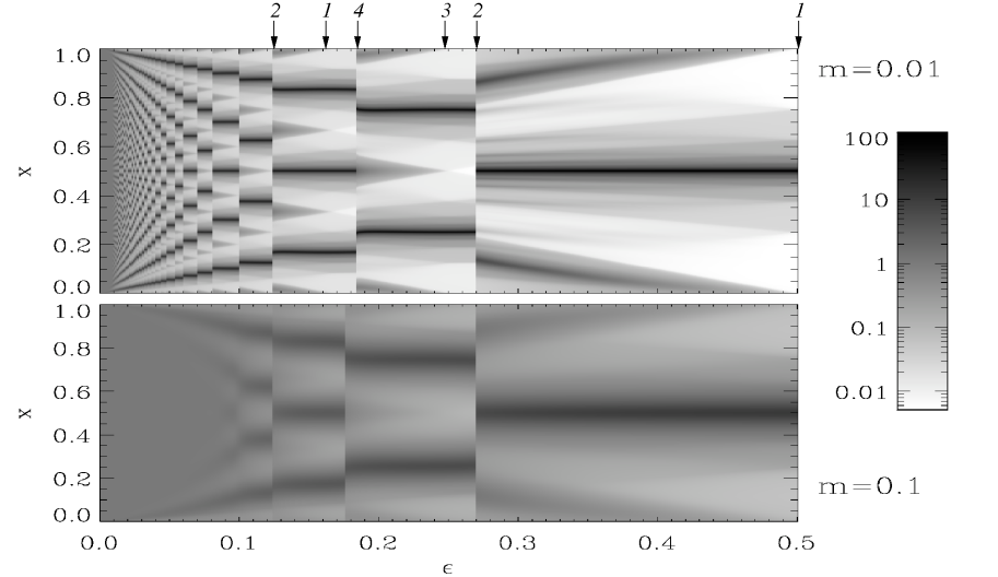
Figure 2: Plot, in a logarithmic grey scale, of the asymptotic probability distributions $P_{\infty}(x)$ as functions of $\epsilon$, obtained after a numerical integration of the master equation (8) for $m=0.01$, top panel, and $m=0.1$, bottom panel. We have used a fourth-order Runge-Kutta method with a time step $\Delta t=0.1$ for the time evolution and Simpson’s rule for the integrals in $x$-space with a discretization $\Delta x=1/M$, $M=2000$. We have checked in some tests cases that smaller time or discretization steps do not change significantly the results. As in Fig.1 we show by arrows the location of the bifurcation points.

The Appendix contains a derivation of the master equation, Eq. (8), appropriate for this process. We have first obtained the asymptotic distribution $P_{\infty}(x)=\lim_{t\to\infty}P(x,t)$ of the master equation starting from a suitable initial condition $P(x,t=0)$. As in other studies, we assume that the initial condition represents a uniform distribution in opinion space, i.e. $P(x,t=0)=1$ for $x\in[0,1]$ and $P(x,t=0)=0$ otherwise. For $m=0$ the steady-state distribution $P_{\infty}(x)$ it is a sum of delta-functions located at particular points. In the case $m>0$ the steady distributions are no longer delta-functions but still are peaked around some particular values if $\epsilon$ is not too small or $m$ not too large. We have plotted in Fig. 2 the master equation steady probability distributions $P_{\infty}(x)$ as a function of the parameter $\epsilon$ for two different values of the noise intensity. In the small noise case $m=0.01$ it is still possible, for not too small $\epsilon$, to identify the same type of bifurcations than in the noiseless case by looking at the maxima of the probability distributions: a type-1 bifurcation at $\epsilon=0.5$ where minor groups begin to form at $x=0$ and $x=1$; a type-2 bifurcation at $\epsilon\approx 0.2695$ where the distribution switches from having one single maximum at $x=0.5$ to having two maxima of equal height located at $x\approx 1/4$ and $x\approx 3/4$; a type-3 bifurcation at $\epsilon\approx 0.250$ where a central maximum begins to grow; a type-4 bifurcation at $\epsilon\approx 0.1835$ where three equally spaced maxima of equal height at $x\approx 1/6$, $x=1/2$ and $x\approx 5/6$ appear. This pattern of bifurcations repeats as $\epsilon$ decreases even further. However, type-1 and type-3 bifurcations are somewhat ambiguous to define since the relative importance of the minor groups actually increases continuously instead of sharply increasing when new maxima begin to form. It is worth stressing that, at variance with the noiseless case, the location of the major groups (defined as the absolute maxima of the distribution) does not vary with $\epsilon$ until a new bifurcation of type-2 or type-4 is reached. These maxima are regularly located at $x\approx 1/k,3/k,\dots,(k-1)/k$ for $k=2,4,6,\dots$

The same general structure can be observed in the case of larger noise $m=0.1$, although the distributions are much broader now. The location of the main bifurcation points can be located at $\epsilon\approx 0.2965$ (type-2) and $\epsilon\approx 0.1755$ (type-4). The type-1 and type-3 transitions are very imprecisely defined, specially for smaller values of $\epsilon$.

For both noise values, one observes that groups become less defined and finally are replaced by a more or less unstructured distribution for $\epsilon$ below a critical value $\epsilon_{c}$ which increases with $m$. Alternatively, one realizes the existence of a critical value $m_{c}=m_{c}(\epsilon)$, increasing with $\epsilon$, above which the group structure disappears from the steady distribution.

A somehow expected feature that emerges from the data shown in Fig. 2 is that the width of the steady distributions grows with the noise intensity. An explicit expression for the width of the single maximum present when $\epsilon\geq 1$ (so that all individuals are allowed to interact) could be obtained from the master equation, since in this case the moments form a closed hierarchy. Defining the moments $M_{1}$ and $M_{2}$ as in the Appendix, the variance $\sigma^{2}=M_{2}-M_{1}^{2}$ satisfies:

$$\frac{d\sigma^{2}}{dt}=-\sigma^{2}+\frac{m}{12}.$$ (2)

In this limiting case (where the main feature of the model, bounded confidence, has been lost since everybody is able to interact with everybody), the variance reaches a steady-state in which the width increases with noise as $\sigma\sim m^{1/2}$.

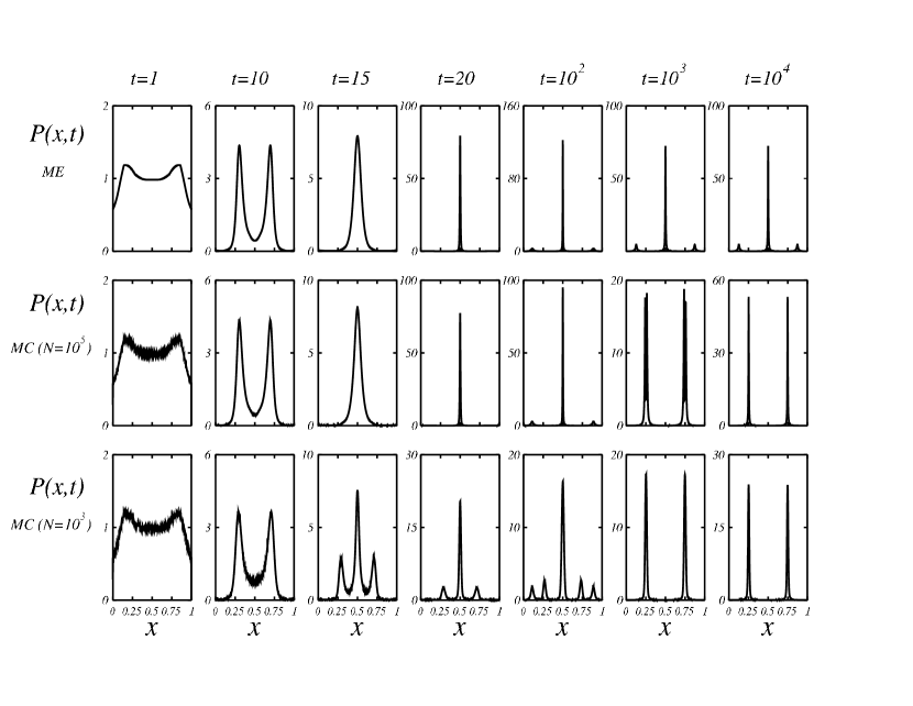
Figure 3: Probability distribution function $P(x,t)$, for intermediate time steps, from Monte-Carlo (MC) simulations (histograms binned with bin size $\Delta x=5\times 10^{-4}$) for two different system sizes $N=10^{3}$ and $N=10^{4}$, and the master equation (ME) integrations of Eq. (8) starting with a flat distribution with $\epsilon=0.28$ and $m=0.01$. The distributions are an average over $10^{5}$ realizations for $N=10^{3}$ and $10^{4}$ realizations for $N=10^{5}$.

3.2 Comparison with Monte-Carlo simulations

Once the master equation predictions have been established, and before comparing with the results coming from the Monte-Carlo numerical simulations using the microscopic rules, a word of warning is, as in the noiseless case, required. In g simulations with a finite number $N$ of individuals the dynamics of the probability distribution as well as its asymptotic, steady-state, values might not coincide with the analysis of the master equation. We have found this deviation to be more pronounced in the case of being close to a bifurcation point. For example, in Fig. 3 we plot the time evolution of the probability coming from Monte-Carlo simulations of the model for different system sizes and the results of the master equation in the case $\epsilon=0.28$, close to a type-2 bifurcation point. It can be seen that, although the Monte-Carlo simulation and the master equation agree initially very well, they start to deviate after a time that depends on the number of individuals $N$: the larger $N$, the longer the time than the Monte-Carlo simulations are faithfully described by the master equation. In this particular case, $\epsilon=0.28$, it can be seen that the master equation agrees with the Monte-Carlo simulations up to a time $t\sim 10$ for $N=10^{3}$ and a time $t\sim 100$ for $N=10^{5}$. In view of this difference, it is surprising that the Monte Carlo steady-state distributions show only small (although observable) finite-size effects. Quite similar functions describe the steady-state data for both $N=10^{3}$ and $N=10^{5}$, see Fig. 4. As can be seen in Fig. 3, however, while the numerical solution of the master equation tends to the steady-state distribution $P_{\infty}(x)$, the Monte-Carlo simulations tend to another distribution, $P_{st}(x)$. These two distributions are very different: $P_{\infty}(x)$ has a large maximum (large group) at $x=0.5$ and two much smaller maxima at $x\approx 0.127$ and $x\approx 0.873$, whereas $P_{st}(x)$ has two equal maxima at $x\approx 0.25$ and $x\approx 0.75$. Although surprising at first, it turns out that the steady-state distribution $P_{st}(x)$ coming from the Monte-Carlo simulations of the model is also very close to a steady-state solution of the master equation (8) having two major groups. However, this last steady-state solution can not be obtained as an asymptotic solution of the master equation $\lim_{t\to\infty}P(x,t)$ starting from a uniform initial condition $P(x,t=0)=1$ for $x\in[0,1]$. It turns out that it is reached when starting instead from an initial condition asymmetric with respect to the center of the interval.

Summing up, for $\epsilon=0.28$ there are two steady-state solutions of the master equation, $P_{st}(x)$ and $P_{\infty}(x)$. Starting from a uniform initial condition, $P_{\infty}(x)$ is the one asymptotically reached as a solution of the master equation. However, $P_{st}(x)$ is, up to finite-size effects, the one reached instead in the Monte-Carlo simulations. We interpret this in terms of the relative stability of both solutions: introducing a fluctuation $\delta P(x)$ on the solution $P_{\infty}(x)$ it is then possible to reach the solution $P_{st}(x)$, but not the reverse. This fluctuation $\delta P(x)$ needs to be asymmetric, $\delta P(x)\neq\delta P(1-x)$ and it appears naturally in Monte-Carlo simulations because of the finite number of individuals $N$ and it is more probable the smaller the value of $N$. This explains that the system with smaller $N$ deviates earlier from the solution of the master equation. If one induces artificially such a non-symmetric perturbation in the solution $P_{\infty}(x)$ or, alternatively, one starts with a non-uniform, asymmetric initial condition, then the master equation tends to $P_{st}(x)$.

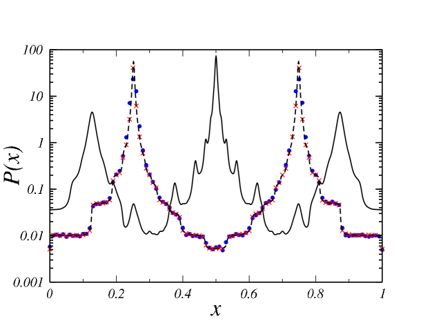
Figure 4: The symbols denote the steady-state probability distribution function $P_{st}(x)$, obtained from Monte-Carlo simulations for system sizes $N=10^{3}$ ($\cdot$) and $N=10^{5}$ ($\times$) in the case $\epsilon=0.28$, $m=0.01$. The dashed line is obtained as an asymptotic solution of the master equation starting with a non-uniform initial condition. These three distributions are very similar in this logarithmic scale, although there are differences in the height of the maxima (see Fig. 3). It turns out that close to each of the two maxima, the distributions can be well fitted by a Lorentzian function[19]. The solid line is the distribution $P_{\infty}(x)$ coming from a numerical solution of the master equation Eq. (8) starting with a uniform distribution.

The existence of more that one steady solution of the master equation seems to be a general feature. In fact, if the distributions in Fig. 2 are recalculated by slowly increasing and decreasing $\epsilon$ without resetting the initial condition to $P(x,t=0)=1$ after each change in $\epsilon$, we observe the hysteresis behavior typical of bistability occurrence close to first-order transitions. Which one of the possible steady solutions is observed in the Monte-Carlo simulations depends on the parameter $\epsilon$. It could even happen that the inherent fluctuations of a finite system take it from one solution to another and back. This sort of bistability is observed, for instance, in Monte-Carlo simulations at $\epsilon=0.31$. As shown in Fig. 5, the evolution displays multiple jumps between two solutions: one with two maxima of equal height and another one with a large central maximum and two smaller maxima near the edges of the opinion interval.

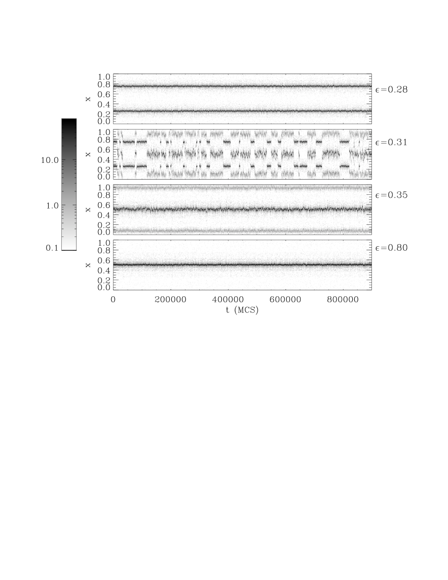
Figure 5: Time series of the opinion distributions $P(x,t)$ at four values of $\epsilon$ and $m=0.01$ and $N=1000$. Grey scale is logarithmic, with values smaller than 0.1 plotted in white. Simulations are initialized with random homogeneous distributions 1000 MCS before the first time shown in the plots. The three first panels are near a type-2 bifurcation. At $\epsilon=0.28$ the system appears polarized in two opinion groups. At $\epsilon=0.35$ a single major opinion has been established, with two lateral minor groups. At $\epsilon=0.31$ the systems fluctuates between these two states. A single group is observed at large $\epsilon$ (bottom panel).

Looking at Fig. 2, one can see that for small $\epsilon$ or, alternatively, for noise intensity $m$ larger than a critical value $m_{c}$ which increases with $\epsilon$, the bifurcations become blurred and the maxima of the distributions are not evident, implying the inhibition of group formation. This happens at $\epsilon\lesssim 0.1$ for $m=0.1$ and at $\epsilon\lesssim 0.01$ for $m=0.01$. A similar effect can be observed in the Monte-Carlo simulations and can be described in terms of an order-disorder transition: order identified with the state with well defined opinion groups and disorder identified with the state without groups. To define in a more quantitative way this transition, we have used the so-called group coefficient $G_{M}$, which aims to characterize the existence of groups [26]. The definition of the group coefficient $G_{M}$ starts by dividing the opinion space $[0,1]$ in $M$ equal boxes and counting the number of individuals $l_{i}$ which, at time step $n$, have their opinion in the box $[(i-1)/M,i/M]$. One next introduces an entropy-like measure $S_{M}=-\sum_{i=1}^{M}\frac{l_{i}}{N}\ln\frac{l_{i}}{N}$. Note that $0\leq S_{M}\leq\ln M$, and that the minimum value $S_{M}$ is obtained when all the individuals are in just one box, while the maximum value, $S_{M}=\ln M$, is reached when $l_{i}=N/M$, i.e. when the opinions are uniformly distributed in the interval $[0,1]$. Finally, the opinion group coefficient is defined as [26]

$$G_{M}=M^{-1}\left\langle e^{\overline{S}_{M}}\right\rangle,$$ (3)

where the over-bar denotes a temporal average in steady conditions and $\langle\cdot\rangle$ indicates an average over different realizations of the dynamics. Note that $1/M\leq G_{M}\leq 1$. Large values $G_{M}\approx 1$ indicate that the opinions are evenly distributed along the full opinion space (a situation identified with disorder), while small values of $G_{M}$ indicate that opinions peak around a finite set of major opinion groups (a situation identified with order).

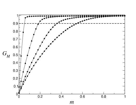
Figure 6: Opinion group coefficient $G_{M=100}$ versus $m$ for $\epsilon=0.05$, $0.2$, $0.4$, and $0.6$, from left to right, respectively as obtained from Monte-Carlo simulations with $N=10^{5}$ individuals (dots, the solid line is a guide to the eye). The location of the order-disorder transition is defined as the value $m_{c}$ for which $G_{M}=0.9$. Note that $m_{c}$ is an increasing function of $\epsilon$ and that the transition is very abrupt for small $\epsilon$.

The data coming from Monte-Carlo simulations, see Fig. 6, show that $G_{M}$ is an increasing function of the noise intensity $m$ and saturates to its maximum value $G_{M}\approx 1$ for large enough values of $m$. The transition from group formation to disorder will be defined, somehow arbitrarily but precisely, as the value $m_{c}$ of the noise intensity for which the group coefficient reaches the value $G_{M}=0.9$. For small values of the confidence parameter $\epsilon$ the transition to the homogeneous state is abrupt and occurs for small values of $m$. If one increases $\epsilon$, the transition becomes less abrupt and a higher noise intensity is needed to obtain the homogeneous, group-free, state. This last feature can be explained by the linear stability analysis that we shall develop in the next section.

4 Linear stability analysis

We have shown that opinion groups still form in presence of small amounts of noise, but an unstructured state without groups dominates the opinion space for noise larger than a critical noise intensity $m_{c}$. Although the transition to group formation is a nonlinear process, one can still derive approximate analytical conditions for the existence of group formation in the parameter space ($\epsilon,m$) by performing a linear stability analysis of the unstructured solution of Eq. (8). This is greatly simplified if one neglects the influence of the boundaries and assumes that the interval $[0,1]$ is wrapped on a circle, i.e. there are periodic boundary conditions at the ends of the interval. This would be a reasonable approximation to describe the distribution far from the boundaries if $\epsilon$, which fixes the interaction range, is sufficiently small. In this case the homogeneous configuration $P_{h}(x)=1$ is an approximation to the unstructured steady solution of the master equation. Analysis of its stability begins by introducing $P(x,t)=P_{h}(x)+A_{q}e^{iqx+\lambda_{q}t}$, where $q$ is the wave number of the perturbation, $\lambda_{q}$ its growth rate and $A_{q}$ the amplitude. After introducing this ansatz in Eq. (8) we find the dispersion relation giving the growth rate of mode $q$:

$$\lambda_{q}=4\epsilon(1-m)\left[\frac{4\sin(q\epsilon/2)}{q\epsilon}-\frac{\sin(q\epsilon)}{q\epsilon}-1\right]-m.$$ (4)

This is plotted in Fig. 7(a), for several values of $m$. The maximum value of $\lambda_{q}$ occurs at $q_{max}=2.7907/\epsilon$. It turns out that he maximum value $\lambda_{q_{max}}$ is negative for $m>m_{c}$ and positive for $\displaystyle m<m_{c}=\frac{\epsilon}{a+\epsilon}$ with $a\approx 0.8676$. Alternatively, for fixed $m$ the maximum growth rate is negative for $\displaystyle\epsilon<\epsilon_{c}=\frac{am}{1-m}$, and positive for $\epsilon>\epsilon_{c}$. Therefore, the homogeneous state is unstable and group formation is possible only for $m<m_{c}$ or $\epsilon>\epsilon_{c}$. The numerical values are $\epsilon_{c}=0.096$ for $m=0.1$ and $\epsilon_{c}=0.0088$ for $m=0.01$, in reasonable agreement with the behavior observed for the master equation dynamics in Fig. 2. Comparison with Monte-Carlo simulations is performed in Fig. 7(b) where we plot the critical value $m_{c}$ obtained from the group coefficient $G_{M}$ as described earlier. We see in the figure that the agreement is very good for small $\epsilon$ but deviates for larger values. This is consistent with the fact that neglecting boundary effects is expected to be appropriate only for small $\epsilon$. Finally, it is possible to estimate roughly the number of groups $n$ by a simple argument: $n$ is related to the wavelength of the maximum growth as $n=q_{max}/2\pi$ or $n=0.444/\epsilon$ for $\epsilon>\epsilon_{c}$. This result is in qualitative agreement with the $\frac{1}{2\epsilon}$-rule, which says that the number of major groups after group formation is roughly determined as the integer part of $\frac{1}{2\epsilon}$ (see [20, 21] for details).

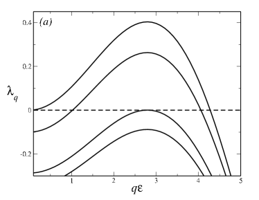
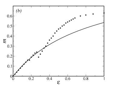
Figure 7: (a) Growth rate, Eq. (4), of a perturbation to the homogeneous solution as a function of $q\epsilon$ for $\epsilon=0.35$ and $m=0.0$, $0.10$, $0.287$, and $0.35$ from top to bottom. It shows that $\lambda_{q}$ becomes negative for high values of $m$. (b) Phase diagram on the plane ($\epsilon,m$) as coming from Monte-Carlo simulations with $N=10^{5}$ individuals (dots), using the criterion based on the group coefficient $G_{M=100}$ as described in the text. The solid line is the prediction of the linear stability analysis. Groups appear below the lines, whereas the unstructured state is stable above.

5 Summary and conclusions

In this paper we have studied the Deffuant et al. model for continuous–opinion dynamics under the presence of noise. Besides the usual rules of the model, we give each individual the opportunity to change, with a certain probability $m$, his opinion to a randomly selected opinion inside the whole opinion space. The final behavior depends of the confidence or interaction parameter $\epsilon$ and the noise intensity $m$.

We have first reviewed the original noiseless version of the model. We have shown that for small number of individuals $N$ and depending of the particular realizations, the exact location of the opinion groups might vary with respect to the predictions of the master equation. In particular, minor groups might not appear and there could be realizations in which even the number of observed major groups differs from the prediction of the master equation.

We have derived (Appendix) a master equation for the probability density function $P(x,t)$ which determines the individuals density or distribution in the opinion space. Numerical integration of this equation from uniform initial conditions reveals that for $m>0$ the steady distributions are no longer delta-functions as for $m=0$, but are still peaked around some well defined maximum value, with some non-vanishing width. By looking at those maxima we are able to identify the same type of bifurcations than in the noiseless case [12, 20]. At variance with the noiseless case, the location of the maxima (the central opinion of the groups) does not depend on $\epsilon$ until a new bifurcation point is reached.

We have also found that in the noisy case the asymptotic steady-state probability distributions reached by Monte-Carlo simulations might not coincide with the ones obtained from the master equation dynamics starting from the same symmetric initial condition. This deviation is more pronounced in the case of being close to a bifurcation point. In particular, we have presented a situation where, starting from a uniform initial condition, a particular stationary distribution, $P_{\infty}(x)$, is actually reached by the master equation but another distribution , $P_{st}(x)$, is the one reached instead in Monte-Carlo simulations. The time in which the Monte-Carlo simulations begin to deviate from the master equation depends on system size: the smaller the size, the earlier the deviation occurs although the final Monte-Carlo distribution $P_{st}(x)$ shows only small size effects. Remarkably, $P_{st}(x)$ turns out to be close to another steady solution of the master equation. Thus, the discrepancy observed during the dynamics does not seem to be simply a trivial finite-$N$ effect. We interpret it in terms of the relative stability of both solutions by adding an asymmetric perturbation to $P_{\infty}(x)$. It is then possible to reach the solution $P_{st}(x)$ obtained from Monte-Carlo simulations, but not the other way around . Asymmetric fluctuations appear naturally in Monte-Carlo dynamics because of the finite number of individuals, and are larger for smaller $N$. We have also shown that the fluctuations present in Monte-Carlo simulations are even able to induce jumps from one solution to another and back.

An order-disorder transition to group formation induced by noise has been characterized using the so-called group coefficient $G_{M}$ for the simulations performed with Monte-Carlo dynamics. We have found that $G_{M}$ is an increasing function of the noise intensity $m$ and saturates to its maximum value $G_{M}\approx 1$ for large enough values of $m$. For small values of the confidence parameter $\epsilon$ the transition to the disordered state is abrupt and occurs for small values of $m$. If one increases $\epsilon$, the transition becomes less abrupt and a higher noise intensity is needed to obtain this state. Using a linear stability analysis of the unstructured (no groups) solution of the master equation we have derived approximate conditions for opinion group formation as a function of the relevant parameters of the system. We have found qualitative agreement between the linear stability analysis and numerical simulations. The agreement is better for small values of $\epsilon$ where boundary effects, neglected to make feasible the linear analysis, are less important. However, we should emphasize that the pattern selection of this model is, with noise and without it, intrinsically a nonlinear phenomenon and obtaining the exact critical conditions for opinion group formation remains a challenge.

Our work stresses the importance that fluctuations and finite-size effects have in the dynamics of social systems for which the thermodynamic limit is not justified [25]. Further work will address the effect that these ingredients have in the dynamics of continuous–opinion models in the presence of an external influence, or forcing, representing the role of advertising.

Appendix

Here we derive the master equation, i.e. the evolution equation for $P_{n}(x)$, the probability density function (pdf) of the opinions at step $n$ for the model introduced in this paper. Note that $P_{n}(x)$ is constructed from the histogram of all individual opinions $x^{i}_{n}$ at step $n$. Let us first find the evolution of the pdf for those two particular individuals $i,j$ that have been selected for updating at step $n$ according to the basic rule Eq. (1). We will denote by $P^{i}_{n+1}(x)$ the pdf of the opinion of individual $i$ at the step $n+1$, i.e the probability that $x^{i}_{n+1}$ adopts the value $x$. According to that rule, it is straightforward to derive the evolution equation

$$P^{i}_{n+1}(x) =\int_{|x^{i}_{n}-x^{j}_{n}|<\epsilon}dx^{i}_{n}dx^{j}_{n}P_{n}(x^{i}_{n})P_{n}(x^{j}_{n})\delta\left(x-\frac{x^{i}_{n}+x^{j}_{n}}{2}\right)$$ (5)

$$+\int_{|x^{i}_{n}-x^{j}_{n}|>\epsilon}dx^{i}_{n}dx^{j}_{n}P_{n}(x^{i}_{n})P_{n}(x^{j}_{n})\delta(x-x^{i}_{n}),$$

and a similar expression for $P^{j}_{n+1}(x)$. The integrals over $x{{}^{i}}_{n}$ and $x{{}^{j}}_{n}$ run both over the interval $[0,1]$. In this equation an independence approximation for the variables $x^{i}_{n},x^{j}_{n}$ has been implicitly assumed, i.e. their joint pdf $P_{n}(x^{i}_{n},x^{j}_{n})$ is supposed to factorize as $P_{n}(x^{i}_{n},x^{j}_{n})=P_{n}(x^{i}_{n})P_{n}(x^{j}_{n})$. This is an uncontrolled approximation whose validity can only be established by an ulterior comparison with the Monte-Carlo simulation of the microscopic rules. For the individuals $k\neq i,j$ whose opinion does not change at time step $n+1$ we have simply $P^{k}_{n+1}(x)=P^{k}_{n}(x)$.

The pdf $P_{n+1}(x)$ has several contributions: (i) With probability $1-m$ two individuals, say $i,j$, are chosen for updating according to the basic evolution rule Eq. (1) and $N-2$ variables remain unchanged. (ii) With probability $m$ one individual is chosen for updating according to the noise rule and $N-1$ variables remain unchanged; the new opinion of the selected individual is sampled from an, in principle, arbitrary distribution $P_{a}(x)$, although in this paper we have taken throughout that $P_{a}(x)$ is the uniform distribution $P_{h}(x)=1$ in the interval $[0,1]$. After consideration of these contributions we are led to the evolution equation

$$P_{n+1}(x) =(1-m)\left[\frac{N-2}{N}P_{n}(x)+\frac{1}{N}P^{i}_{n+1}(x)+\frac{1}{N}P^{j}_{n+1}(x)\right]$$ (6)

$$+m\left[\frac{N-1}{N}P_{n}(x)+\frac{1}{N}P_{a}(x)\right].$$

Replacing $P^{i}_{n+1}(x)$ and $P^{j}_{n+1}(x)$ from Eq. (5) one obtains after some algebra

$$P_{n+1}(x) =P_{n}(x)+\frac{(1-m)}{N}\left[4\int_{|x-x^{\prime}|<\epsilon/2}dx^{\prime}P_{n}(2x-x^{\prime})P_{n}(x^{\prime})\right.$$ (7)

$$\left.-2P_{n}(x)\int_{|x-x^{\prime}|<\epsilon}dx^{\prime}P_{n}(x^{\prime})\right]+\frac{m}{N}\left[P_{a}(x)-P_{n}(x)\right].$$

The integrals over $x^{\prime}$ run over the interval $[0,1]$, and it has to be imposed that $P_{n}(x)=0$ if $x\notin[0,1]$. We now take the continuum limit $P_{n}(x)\rightarrow P(x,t)$ with a time $t=n\Delta t$ and taking the limit $\Delta t=1/N\rightarrow 0$ as $N\rightarrow\infty$, to obtain:

$$\frac{\partial P(x,t)}{\partial t} =(1-m)\left[4\int_{|x-x^{\prime}|<\epsilon/2}dx^{\prime}P(2x-x^{\prime},t)P(x^{\prime},t)\right.$$ (8)

$$\left.-2P(x,t)\int_{|x-x^{\prime}|<\epsilon}dx^{\prime}P(x^{\prime},t)\right]+m\left[P_{a}(x)-P(x,t)\right],$$

which is the master equation of the Deffuant et al. model in the presence of noise and the basis of our analysis. The noiseless case, $m=0$, was first obtained in reference [12]. We note here the symmetry property of the master equation: if the initial condition is symmetric around the central point $x=1/2$, namely that $P(x,t=0)=P(1-x,t=0)$, then this property holds for any later time, $P(x,t)=P(1-x,t),\forall t>0$.

The time evolution of the first moments of $P(x,t)$ can be computed from the master equation. Defining the moments as $M_{k}(t)=\int dxx^{k}P(x,t)$ one finds easily that $\displaystyle\frac{dM_{0}}{dt}=0$ (normalization condition) and that the first moment evolves as $\displaystyle\frac{dM_{1}}{dt}=m\left(M_{1}^{a}-M_{1}\right)$, being $M_{1}^{a}$ the first moment of the distribution $P_{a}(x)$. Therefore, if $m>0$, the average opinion tends to $M_{1}=M_{1}^{a}$ independently of the initial condition, and it is always conserved in the noiseless case $m=0$. Expressions for higher-order moments can only be obtained in the special case $\epsilon\geq 1$, as discussed in the main text.

References

References

- [1] Castellano C, Fortunato S and Loreto V, 2009 Rev. Mod. Phys. 81, 591
- [2] Stauffer D, 2005 AIP Conf. Proc. 779, 56
- [3] S. Galam S, 2002 Eur. Phys. J. B 25, 403
- [4] F. Schweitzer and J. Holyst, 2000 Eur. Phys. J. B 15, 723
- [5] K Sznajd-Weron and J. Sznajd, 2000 Int. J. Mod. Phys. C 11, 1157
- [6] Deffuant G, Neu D, Amblard F, and Weisbuch G, 2000 Adv. Compl. Syst. 3, 87
- [7] Weisbuch G, Deffuant G, Amblard F, and Nadal J P, 2002 Complexity 7, 855
- [8] Weisbuch G, Deffuant G, and Amblard F, 2005 Physica A 353, 555
- [9] Hegselmann R and Krause U, 2002 J. Artif. Soc. Soc. Simul. 5, 2.
- [10] Axelrod R, 1997 J. Conflict Res. 41, 203
- [11] Granovetter M, 1978 American Journal of Sociology 83, 1420
- [12] Ben-Naim E, Krapivsky P L, and Redner S, 2003 Physica D 183, 190
- [13] Amblard F and Deffuant G, 2004 Physica A 343, 725
- [14] Stauffer D, Sousa A, and Schulze C, 2004 J. Artif. Soc. Soc. Simul. 7, 7
- [15] B. Kozma and A. Barrat, 2008 Phys. Rev. E 77, 016102
- [16] Guo L and Cai X, 2009 Commun. Comput. Phys. 5, 1045
- [17] Carletti T, Fanelli D, Grolli S, and Guarino A, 2006 Europhys. Lett 74, 222
- [18] Carletti T, Fanelli D, Guarino A, Bagnoli F, and Guazzinni A, 2008 Eur. Phys. J. B 64, 285
- [19] Ben-Naim E, 2005 Europhys. Lett 69, 671
- [20] Lorenz J, 2005 Physica A 355, 217
- [21] Lorenz J, 2007 Int. J. Mod. Phys. C 18, 1819
- [22] Lorenz J, PhD thesis, Universität Bremen, 2007. http://nbn-resolving.de/urn:nbn:de:gbv:46-diss000106688.
- [23] Laguna M F, Abramson G, and Zanette D H, 2004 Complexity 9, 31
- [24] Porfiri M, Bollt E M, and Stilwell D J, 2007 Eur. Phys. J. B 57, 481
- [25] Toral R and Tessone C J, 2007 Comm. Comp. Phys. 2 177
- [26] López C, 2004 Phys. Rev. E 70, 066205