Homogenization of composites with interfacial debonding using duality-based solver and micromechanics

Abstract.

One of the key aspects governing the mechanical performance of composite materials is debonding: the local separation of reinforcing constituents from matrix when the interfacial strength is exceeded. In this contribution, two strategies to estimate the overall response of particulate composites with rigid-brittle interfaces are investigated. The first approach is based on a detailed numerical representation of a composite microstructure. The resulting problem is discretized using the Finite Element Tearing and Interconnecting method, which, apart from computational efficiency, allows for an accurate representation of interfacial tractions as well as mutual inter-phase contact conditions. The candidate solver employs the assumption of uniform fields within the composite estimated using the Mori-Tanaka method. A set of representative numerical examples is presented to assess the added value of the detailed numerical model over the simplified micromechanics approach.

Keywords

first-order homogenization; particulate composites; debonding; FETI method; micromechanics

1. Introduction

Particle-reinforced composites, and the fibrous composites in particular, present a progressive class of materials with a steadily increasing importance in virtually all areas of structural engineering, e.g., [7, 30]. It is now being generally accepted that one of the key factors governing the mechanical performance of composite materials is the interfacial debonding: the partial separation of reinforcements from matrix phase when the surface tractions locally exceed the interfacial strength. Therefore, a considerable amount of research effort has been invested into the development of a realistic model for debonding-induced damage processes in heterogeneous media in the field of materials science and engineering. Two major classes of models are currently available: (i) computational homogenization methods and (ii) micromechanics-based approaches. In spite of significant advances in understanding the debonding phenomenon accomplished in recent decades, both modelling approaches still suffer from certain limitations.

The essential goal of the computational homogenization is to determine the detailed distribution of local fields within a characteristic heterogeneity pattern of the analyzed composites, usually represented by a Periodic Unit Cell (PUC), employing a suitable discretization technique. In the context of the debonding behavior, the most frequent and versatile approach is based on the primal variant of the Finite Element Method (FEM), e.g., [8, 25, 45, and references therein] or a mixed discretization approach such as the Voronoi Cell FEM [24]. Alternative numerical schemes include the Boundary Element Method (BEM)-based homogenization, e.g., [6] or coupled BEM/FEM simulations [15]. The interfacial behavior is, in all the previously mentioned cases, modeled in the form of a traction-separation constitutive law, with the interfacial stiffness as the basic material parameter. Such concept, however, inevitably leads to problems for the perfect particle/matrix bonding, which formally corresponds to the infinite value of interfacial stiffness. In the actual implementation, of course, the perfect bonding case is approximated using a large penalty-like term, deteriorating the conditioning of the numerical problem manifested in spurious traction oscillations and hence inaccurate prediction of damage initiation, see e.g. [2, 37] and references therein for additional discussion. The finite interfacial stiffness, on the other hand, allows for mutual interpenetration of individual constituents, resulting in a non-physical distribution of some of the mechanical fields within composite. To circumvent these problems, an Uzawa-type algorithm combined with the FEM or BEM discretization were employed by Procházka and Šejnoha in [33, 34] to solve a single fiber pull-out problem including interfacial Coloumb friction. Moreover, the primal approaches of computational contact mechanics were used with some success in [40, 46] to homogenize debonding composites. All these studies, however, suffer from an increased computational cost due to non-optimal convergence rates and as such are not well-suited for the fully coupled FE² computational homogenization [14, 21], where the detailed PUC response serves as an “effective” non-linear constitutive relation seen at the coarser scale of resolution.

The micromechanics-based solvers are, on the other hand, typically based on a specific solution of field equations and limited information of a microstructure, such as volume fractions of individual phases. This makes the analytical approaches extremely efficient from the computational point of view; their accuracy is, however, to a major extent influenced by validity of the adopted assumptions. Early contributions to the micromechanical modelling of debonding composites include the contribution of Benveniste [3] and Pagano and Tandon [29], where the original uniform field theories were extended to treat possible field discontinuities at the fiber-matrix interphase. Additional improvements include introduction of compliant interfaces with linear behavior [18], later extended for non-linear constitutive relations [9, 38]. In addition, layered inclusion models combined with simple numerical procedures were introduced in [39] to simulate specific particle-reinforced composites. Several attempts have also been made to increase the predictive capabilities of effective media models by calibrating their response against the results of detailed numerical simulations, e.g. [19, 35, 42]. However, lacking reliable reference numerical solution, due to the reasons summarized above, such a strategy can hardly reproduce the dominant features of the complex interaction mechanisms in the material systems under investigation.

In this contribution, we present an alternative numerical approach to the numerical homogenization of debonding composites, which circumvents the previously mentioned obstacles. The method itself builds on the Finite Element Tearing and Interconnecting (FETI) solver due to Farhat and Roux [13] and adopts recent ideas in duality-based solvers [11, 23, 41] to the computational homogenization setting. The added value of the duality- and FETI-based framework can be summarized as follows:

• For the perfect complete bonding case, the method reduces to the original FETI algorithm; no artificial penalty-like stiffness is therefore needed to enforce the displacement continuity.

• Since interfacial tractions are introduced independently from the displacement fields in the form of Lagrange multipliers, they are captured rather accurately in the whole loading regime. Therefore, the interfacial strength criteria can be directly adopted, cf. [16].

• In addition, the Lagrange multipliers allow us to efficiently treat frictionless contact conditions [10], making the numerical algorithm well-suited for providing reference solutions to micromechanics schemes.

• As typical of FETI-based methods, the dual problem involves the interface-related quantities only. This not only reduces the problem complexity by an order of magnitude, but also introduces a natural coarse level to the numerical algorithm [10, 12], which opens the way to efficient and scalable iterative solvers.

In the rest of this work, these claims are clarified in more details by addressing the fundamental case of composites with rigid-perfectly brittle interfaces in the two-dimensional setting. The paper starts with a brief overview of the first-order periodic homogenization of composites with imperfect bonding of phases in Section 2. The numerical resolution of the unit cell problem using the FETI method is covered in Section 3, while a simple micromechanical model based on the Mori-Tanaka method is introduced in Section 4. Performance of both approaches is compared in Section 5 for both regular as well as disordered real-world microstructures. Finally, the most important results are summarized in Section 6.

In the whole text, representation of the symmetric second and fourth-order tensors of the Mandel type is systematically employed. In particular, $a$, $\boldsymbol{a}$ and $\mathbf{a}$ denote a scalar value, a vector or a matrix, respectively and the matrix representations are defined, in the two-dimensional setting, via

$$\boldsymbol{a}=\left[\begin{array}[]{c}a_{11}\\ a_{22}\\ \sqrt{2}a_{12}\end{array}\right], \mathbf{a}=\left[\begin{array}[]{ccc}a_{1111}&a_{1122}&\sqrt{2}a_{1112}\\ a_{1122}&a_{2222}&\sqrt{2}a_{2212}\\ \sqrt{2}a_{112}&\sqrt{2}a_{2212}&2a_{1212}\\ \end{array}\right],$$ (7)

cf. [27, Section 2.3]. Other symbols and abbreviations are introduced in the text as needed.

2. Overview of periodic homogenization

In the current Section, the basic notation and essentials of the first-order periodic homogenization theory are briefly summarized, with the aim to provide a continuous setting compatible with the FETI-based discretization discussed next. For more detailed treatment of individual steps, an interested reader is referred to [17, 26].

2.1. Geometry of PUC and averaging

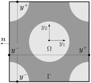
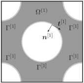
Figure 1. Decomposition of a PUC; (a) Unit cell, (b) matrix phase, (c) inclusion (fiber).

Consider a Periodic Unit Cell (PUC) representing a cross-section of composite material with long fibers, see Figure 1. Formally, the PUC is understood as an open set $\Omega\subset{\mathbb{R}}^{2}$ with boundary $\Gamma$. Within the PUC, we distinguish $n$ disjoint sub-domains $\Omega^{(i)}$. In the following text, the index $i=1$ will be reserved for the multiply-connected matrix phase, whereas simply-connected non-overlapping heterogeneities, i.e. fibers, are enumerated by $i=2,3,\ldots,n$. It will also prove useful to introduce the internal interfaces (denoted by square brackets instead of round ones):

$$\Gamma^{[j]}=\overline{\Omega^{(1)}}\cap\overline{\Omega^{(j)}}, {\Gamma^{[1]}}=\bigcup_{j=2}^{n}{\Gamma^{[j]}},$$ (8)

i.e. the boundary $\Gamma^{[j]}$ corresponds to the interface between $j$-th fiber and the matrix phase, while $\Gamma^{[1]}$ is reserved for the whole internal matrix interface, cf. Figures 1 and 1. The normal to the set $\Omega$, defined on the whole boundary $\Gamma$, is referred to as $\boldsymbol{n}$ with the appropriate adjustment for internal boundaries. Note that for any $\boldsymbol{y}\in\Gamma^{[j]}$, the associated normals for the matrix phase and the $j$-fiber verify

$$\boldsymbol{n}^{[1]}(\boldsymbol{y})=-\boldsymbol{n}^{[j]}(\boldsymbol{y}),$$ (9)

cf. Figures 1 and 1.

Finally, we fix a nomenclature related to the determination of averages for possibly discontinuous fields defined on PUC. To that end, consider a collection of functions $f^{(i)}$ defined independently on sub-domains $\Omega^{(i)}$, jointly denoted as

$$f\left(\boldsymbol{y}\right)=\left\{\begin{array}[]{l@{\quad}l}f^{(1)}\left(\boldsymbol{y}\right),&\boldsymbol{y}\in\Omega^{(1)}\\ f^{(2)}\left(\boldsymbol{y}\right),&\boldsymbol{y}\in\Omega^{(2)}\\ \lx@intercol\hfil\vdots\hfil\lx@intercol\\ f^{(n)}\left(\boldsymbol{y}\right),&\boldsymbol{y}\in\Omega^{(n)}\end{array}\right..$$ (10)

Then, given two functions $f$ and $g$, we introduce the averaging relation in the form, cf. [26, Section 2]:

$${\left\langle\frac{\partial f(\boldsymbol{y})}{\partial y_{k}}g(\boldsymbol{y})\right\rangle}=\frac{1}{{|\Omega|}}\sum_{i=1}^{n}\left(\int_{\Omega^{(i)}}\frac{\partial f^{(i)}(\boldsymbol{y})}{\partial y_{k}}g^{(i)}(\boldsymbol{y}){\mathrm{\,d}{\Omega}}-\int_{\Gamma^{[i]}}f^{[i]}(\boldsymbol{y})g^{[i]}(\boldsymbol{y})n^{[i]}_{k}(\boldsymbol{y}){\mathrm{\,d}{{\Gamma}}}\right),$$ (11)

where ${|\Omega|}$ stands for the area of PUC and, in analogy with Equation (8), $f^{[i]}$ and $g^{[i]}$ denote the traces of functions $f^{(i)}$ and $g^{(i)}$ on $\Gamma^{[i]}$, e.g. [36]. Note that for $\Omega$-continuous functions $f$ and $g$, the second term of the right hand side of (11) vanishes due to identity (9), thus recovering the standard format of the average on the unit cell.

2.2. First-order homogenization framework

In the current work, the strain controlled approach to the first-order computational homogenization (in the terminology introduced in [26]) is adopted. Within this setting, the analysis is split into two independent levels: the microscale corresponding to the behavior on the level of individual constituents and the macroscale providing the overall response of the heterogeneous material under investigation. In the sequel, we restrict our attention to the microscale problem and consider a PUC subject to a macroscopic strain $\boldsymbol{E}$, which, when combined with the governing equations of continuum mechanics and the constitutive description of individual phases, determines the distribution of microscopic fields within the PUC. The average value of the microscopic stress $\boldsymbol{\sigma}$ then yields the value of macroscopic stress $\boldsymbol{\Sigma}$, implicitly defining the homogenized constitutive law.

Following this conceptual lead, we introduce an additive split of displacement and strain fields ${\boldsymbol{u}}$ and $\boldsymbol{\varepsilon}$ in the form:

$${\boldsymbol{u}}^{(i)}(\boldsymbol{y})=\mathbf{X}(\boldsymbol{y}){\sf{}^{T}}\boldsymbol{E}+{{\boldsymbol{u}}^{*}}^{(i)}(\boldsymbol{y}), \boldsymbol{\varepsilon}^{(i)}(\boldsymbol{y})=\mathbf{\boldsymbol{\partial}}{\boldsymbol{u}}^{(i)}(\boldsymbol{y})=\boldsymbol{E}+{\boldsymbol{\varepsilon}^{*}}^{(i)}(\boldsymbol{y}),$$ (12)

where the first part of the decompositions (12) corresponds to an affine displacement field due to $\boldsymbol{E}$, whereas the second part is the correction due to the heterogeneity of the PUC. The matrices $\mathbf{X}$ and $\mathbf{\boldsymbol{\partial}}$ are defined in slightly different form than in the standard approach [5]

$$\mathbf{X}(\boldsymbol{y})=\left[\begin{array}[]{cc}y_{1}&0\\ 0&y_{2}\\ \frac{1}{\sqrt{2}}y_{2}&\frac{1}{\sqrt{2}}y_{1}\end{array}\right], \mathbf{\boldsymbol{\partial}}=\left[\begin{array}[]{cc}\frac{\partial}{\partial y_{1}}&0\\ 0&\frac{\partial}{\partial y_{2}}\\ \frac{1}{\sqrt{2}}\frac{\partial}{\partial y_{2}}&\frac{1}{\sqrt{2}}\frac{\partial}{\partial y_{1}}\end{array}\right],$$ (19)

due to the adopted Mandel notation.

In general, two conditions need to be satisfied to arrive at a thermodynamically consistent macro-micro coupling. We start from the macro-micro strain compatibility condition

$${\left\langle\boldsymbol{\varepsilon}(\boldsymbol{y})\right\rangle}=\boldsymbol{E},$$ (20)

transformed using Equation (12) and the integration formula (11) into a generalized boundary conditions

$${\left\langle\boldsymbol{\varepsilon}^{*}(\boldsymbol{y})\right\rangle}=\boldsymbol{0} \Longleftrightarrow \oint_{\Gamma}\mathbf{\boldsymbol{\nu}}(\boldsymbol{y}){\boldsymbol{u}}^{*}(\boldsymbol{y}){\mathrm{\,d}{{\Gamma}}}=\boldsymbol{0},$$ (21)

imposed on the fluctuating displacement field ${\boldsymbol{u}}^{*}$. The $\mathbf{\boldsymbol{\nu}}$ matrix appearing in (21) stores the components of the normal vector and is defined analogously to (19)₁:

$$\mathbf{\boldsymbol{\nu}}(\boldsymbol{y})=\left[\begin{array}[]{cc}n_{1}(\boldsymbol{y})&0\\ 0&n_{2}(\boldsymbol{y})\\ \frac{1}{\sqrt{2}}n_{2}(\boldsymbol{y})&\frac{1}{\sqrt{2}}n_{1}(\boldsymbol{y})\end{array}\right].$$ (22)

The second ingredient of the macro-micro scale transition is provided by the Hill lemma

$$\boldsymbol{E}{\sf{}^{T}}\boldsymbol{\Sigma}={\left\langle\boldsymbol{\varepsilon}(\boldsymbol{y}){\sf{}^{T}}\boldsymbol{\sigma}(\boldsymbol{y})\right\rangle},$$ (23)

imposing the equality of the work of macroscopic and microscopic stresses and strains. Assuming a self-equilibrated microscopic stress field (i.e. $\mathbf{\boldsymbol{\partial}}{\sf{}^{T}}\boldsymbol{\sigma}=\boldsymbol{0}$) and employing the identity (11), the Hill lemma can be transformed into

$${\left\langle{\boldsymbol{\varepsilon}^{*}}(\boldsymbol{y}){\sf{}^{T}}\boldsymbol{\sigma}(\boldsymbol{y})\right\rangle}=0 \Longleftrightarrow \oint_{\Gamma}{{\boldsymbol{u}}^{*}}(\boldsymbol{y}){\sf{}^{T}}\boldsymbol{\lambda}(\boldsymbol{y}){\mathrm{\,d}{{\Gamma}}}=0,$$ (24)

where $\boldsymbol{\lambda}$ denotes the traction vector defined via

$$\boldsymbol{\lambda}(\boldsymbol{y})=\mathbf{\boldsymbol{\nu}}(\boldsymbol{y}){\sf{}^{T}}\boldsymbol{\sigma}(\boldsymbol{y}).$$ (25)

Note that the two conditions (21) and (24) represent the necessary constraints for a consistent macro-micro scale tying. A particularly convenient choice, especially for the adopted periodic setting, is provided by restricting the heterogeneous displacements ${\boldsymbol{u}}^{*}$ to $\Omega$-periodic fields. Then, for any homologous vectors $\boldsymbol{y}^{+}$ and $\boldsymbol{y}^{-}$ located on the boundary $\Gamma$, cf. Figure 1, the periodicity and anti-periodicity of displacement and tractions holds:

$${\boldsymbol{u}}^{*}(\boldsymbol{y}^{+})={\boldsymbol{u}}^{*}({\boldsymbol{y}^{-}}), \boldsymbol{\lambda}(\boldsymbol{y}^{+})=-\boldsymbol{\lambda}(\boldsymbol{y}^{-}),$$ (26)

which, together with the identity $\boldsymbol{n}(\boldsymbol{y}^{+})=-\boldsymbol{n}(\boldsymbol{y}^{-})$, ensures the satisfaction of both kinematic and energetic consistency conditions.

2.3. Unit cell problem

The distribution of the displacements and interfacial tractions follows from the total energy functional in the form:

$$\Pi\left(\widehat{{\boldsymbol{u}}}(\boldsymbol{y}),\widehat{\boldsymbol{\lambda}}(\boldsymbol{y})\right)=\sum_{i=1}^{n}\left({\textstyle\frac{1}{2}}\int_{\Omega^{(i)}}\widehat{\boldsymbol{\varepsilon}}^{(i)}(\boldsymbol{y}){\sf{}^{T}}\mathbf{L}^{(i)}\widehat{\boldsymbol{\varepsilon}}^{(i)}(\boldsymbol{y}){\mathrm{\,d}{\Omega}}-\int_{\Gamma^{[i]}}\widehat{\boldsymbol{\lambda}}_{\ell}^{[i]}(\boldsymbol{y}){\sf{}^{T}}\widehat{{\boldsymbol{u}}}_{\ell}^{[i]}(\boldsymbol{y}){\mathrm{\,d}{\Gamma}}\right),$$ (27)

where the symbol $\mathbf{L}^{(i)}$ stands for the domain-wise constant material stiffness matrix, $\widehat{a}$ is used to denote the trial value of a quantity $a$; ${\boldsymbol{u}}_{\ell}^{[i]}$ and $\boldsymbol{\lambda}_{\ell}^{[i]}(\boldsymbol{y})$ correspond to displacement and traction fields expressed in the local coordinate system as

$$\left[\begin{array}[]{c}u^{[i]}_{n}(\boldsymbol{y})\\ u^{[i]}_{t}(\boldsymbol{y})\end{array}\right] = \left[\begin{array}[]{c}u^{[i]}_{1\ell}(\boldsymbol{y})\\ u^{[i]}_{2\ell}(\boldsymbol{y})\end{array}\right]=\mathbf{T}^{[i]}(\boldsymbol{y})\left[\begin{array}[]{c}u^{[i]}_{1}(\boldsymbol{y})\\ u^{[i]}_{2}(\boldsymbol{y})\end{array}\right],$$ (34)

$$\left[\begin{array}[]{c}\sigma^{[i]}(\boldsymbol{y})\\ \tau^{[i]}(\boldsymbol{y})\end{array}\right] = \left[\begin{array}[]{c}\lambda^{[i]}_{1\ell}(\boldsymbol{y})\\ \lambda^{[i]}_{2\ell}(\boldsymbol{y})\end{array}\right]=\mathbf{T}^{[i]}(\boldsymbol{y})\left[\begin{array}[]{c}\lambda^{[i]}_{1}(\boldsymbol{y})\\ \lambda^{[i]}_{2}(\boldsymbol{y})\end{array}\right],$$ (41)

with $\mathbf{T}^{[i]}$ denoting the transformation matrix related to the $i$-th interface:

$$\mathbf{T}^{[i]}(\boldsymbol{y})=\left[\begin{array}[]{r}\boldsymbol{n}^{[i]}(\boldsymbol{y}){\sf{}^{T}}\\ \boldsymbol{t}^{[i]}(\boldsymbol{y}){\sf{}^{T}}\end{array}\right],$$ (42)

cf. Figures 1 and 2 for an illustration. Employing the displacement and strain decomposition (12) together with the interfacial equilibrium conditions

$$\boldsymbol{\lambda}^{[1]}(\boldsymbol{y})=-\boldsymbol{\lambda}^{[j]}(\boldsymbol{y})\ \forall\boldsymbol{y}\in\Gamma^{[j]}$$ (43)

leads to a modified energy functional

$$\Theta\left(\widehat{{\boldsymbol{u}}}^{*}(\boldsymbol{y}),\widehat{\boldsymbol{\lambda}}^{[1]}(\boldsymbol{y})\right) = \sum_{i=1}^{n}\left({\textstyle\frac{1}{2}}\int_{\Omega^{(i)}}{{\widehat{\boldsymbol{\varepsilon}}^{*}}{{}^{(i)}}}(\boldsymbol{y}){\sf{}^{T}}\mathbf{L}^{(i)}{\widehat{\boldsymbol{\varepsilon}}^{*}}{{}^{(i)}}(\boldsymbol{y}){\mathrm{\,d}{\Omega}}+\int_{\Omega^{(i)}}{{\widehat{\boldsymbol{\varepsilon}}^{*}}{{}^{(i)}}}(\boldsymbol{y}){\sf{}^{T}}\mathbf{L}^{(i)}\boldsymbol{E}{\mathrm{\,d}{\Omega}}\right)$$ (44)

$$+ \sum_{j=2}^{n}\int_{\Gamma^{[j]}}\widehat{\boldsymbol{\lambda}}_{\ell}^{[1]}(\boldsymbol{y}){\sf{}^{T}}\left({\widehat{{\boldsymbol{u}}}^{*}_{\ell}}{{}^{[j]}}(\boldsymbol{y})-{\widehat{{\boldsymbol{u}}}^{*}_{\ell}}{{}^{[1]}}(\boldsymbol{y})\right){\mathrm{\,d}{\Gamma}},$$

defined on the set of kinematically admissible displacements

$${\mathbb{K}}=\left\{\widehat{{\boldsymbol{u}}}^{*}(\boldsymbol{y})\mbox{ is }\Omega\mbox{-periodic},\widehat{{\boldsymbol{u}}}^{*}(\boldsymbol{y})=\boldsymbol{0}\ \forall\boldsymbol{y}\in\Gamma_{\mathrm{D}}\right\},$$ (45)

with $\Gamma_{\mathrm{D}}$ denoting a part of the boundary, typically the corner nodes of a PUC, where the Dirichlet boundary conditions are imposed to prevent the rigid body modes. The admissible interfacial tractions are constrained to the statically admissible set $\Lambda$ discussed in more detail in Section 3.2. The “true” displacement and traction fields then coincide with the saddle point of the functional:

$$\left({\boldsymbol{u}}^{*}(\boldsymbol{y}),\boldsymbol{\lambda}^{[1]}(\boldsymbol{y})\right)=\arg\max_{\widehat{\boldsymbol{\lambda}}^{[1]}(\boldsymbol{y})\in\Lambda}\min_{\widehat{{\boldsymbol{u}}}^{*}(\boldsymbol{y})\in{\mathbb{K}}}\Theta\left(\widehat{{\boldsymbol{u}}}^{*}(\boldsymbol{y}),\widehat{\boldsymbol{\lambda}}^{[1]}(\boldsymbol{y})\right),$$ (46)

thereby defining the unit cell problem for composites with debonding phases.

3. FETI-based solution to unit cell problem

This Section presents an engineering approach to the solution of non-linear debonding problem (46). In particular, a two-step iterative procedure is employed, where in the outer loop, the static admissibility constraint $\widehat{\boldsymbol{\lambda}}^{[1]}\in\Lambda$ is dropped to arrive at the prediction of traction distribution $\tilde{\boldsymbol{\lambda}}^{[1]}$. Next, in the correction step, the trial tractions are transformed into a physically admissible value using an interfacial constitutive law and the loop is repeated until convergence is achieved. It is fair to mention that, when compared to more sophisticated techniques based on quadratic programming [10, 11, 41], the current technique is definitely less robust due to the missing convergence theory. The definite advantage of the algorithm, on the other hand, is its simplicity; as illustrated in the sequel, the implementation systematically employs a standard FETI solver for linear elasticity, see e.g. [22, Chapter 4]. In the sequel, individual steps of the algorithm are summarized in some detail.

3.1. Prediction step

Following the basic idea of the FETI-based discretization [12, 22], the true fields of fluctuating displacements and the corresponding strains are approximated independently on individual domains $\Omega^{(i)}$

$${\boldsymbol{u}}^{*}{{}^{(i)}}(\boldsymbol{y})\approx\mathbf{N}_{u}^{(i)}(\boldsymbol{y})\boldsymbol{d}_{u}^{(i)}, \boldsymbol{\varepsilon}^{*}{{}^{(i)}}(\boldsymbol{y})\approx\mathbf{B}_{u}^{(i)}(\boldsymbol{y})\boldsymbol{d}_{u}^{(i)} \forall\boldsymbol{y}\in\Omega^{(i)},$$ (47)

where $\mathbf{N}_{u}$ denotes the matrix of basis functions, $\mathbf{B}_{u}=\mathbf{\partial}\mathbf{N}_{u}$ is the displacement-to-strain matrix and $\boldsymbol{d}_{u}$ stores the nodal displacements of individual components, e.g. [5]. The discretization of the interfacial tractions in the predictor step is performed analogously:

$$\tilde{\boldsymbol{\lambda}}^{[1]}(\boldsymbol{y})\approx\mathbf{N}_{\lambda}^{[1]}(\boldsymbol{y})\tilde{\boldsymbol{d}_{\lambda}}^{[1]} \forall\boldsymbol{y}\in\Gamma^{[1]}.$$ (48)

Following the standard Ritz-Galerkin procedure, identical basis functions are used for the discretization of the trial values.

After introducing the approximations (47) and (48) into the energy functional (44), the stationarity conditions for $\boldsymbol{d}_{u}^{(i)}$ and $\tilde{\boldsymbol{d}_{\lambda}}^{[1]}$ reduce to a system of linear equations

$$\mathbf{K}^{(i)}\boldsymbol{d}_{u}^{(i)} = \boldsymbol{f}^{(i)}-\mathcal{E}^{(i)}{\sf{}^{T}}\tilde{\boldsymbol{d}_{\lambda}}^{[1]},$$ (49)

$$\sum_{i=1}^{n}\mathcal{E}^{(i)}\boldsymbol{d}_{u}^{(i)} = \boldsymbol{0},$$ (50)

with the individual matrices expressed in the form:

$$\mathbf{K}^{(i)} = \int_{\Omega^{(i)}}\mathbf{B}_{u}^{(i)}(\boldsymbol{y}){\sf{}^{T}}\mathbf{L}^{(i)}\mathbf{B}_{u}^{(i)}(\boldsymbol{y}){\mathrm{\,d}{\Omega}},$$ (51)

$$\boldsymbol{f}^{(i)} = -\int_{\Omega^{(i)}}\boldsymbol{E}{\sf{}^{T}}\mathbf{L}^{(i)}\mathbf{B}_{u}^{(i)}(\boldsymbol{y}){\mathrm{\,d}{\Omega}},$$ (52)

$$\mathcal{E}^{(1)} = -\sum_{j=2}^{n}\int_{\Gamma^{[j]}}\mathbf{T}^{[1]}(\boldsymbol{y}){\sf{}^{T}}\mathbf{N}_{\lambda}^{[1]}(\boldsymbol{y}){\sf{}^{T}}\mathbf{T}^{[1]}(\boldsymbol{y})\mathbf{N}_{u}^{(1)}(\boldsymbol{y}){\mathrm{\,d}{\Gamma}},$$ (53)

$$\mathcal{E}^{(j)} = \int_{\Gamma^{[j]}}\mathbf{T}^{[1]}(\boldsymbol{y}){\sf{}^{T}}\mathbf{N}_{\lambda}^{[1]}(\boldsymbol{y}){\sf{}^{T}}\mathbf{T}^{[1]}(\boldsymbol{y})\mathbf{N}_{u}^{(j)}(\boldsymbol{y}){\mathrm{\,d}{\Gamma}}.$$ (54)

The solution of Equation (49) exists only if and only if

$$\mathbf{R}^{(i)}{\sf{}^{T}}\left(\boldsymbol{f}^{(i)}-\mathcal{E}^{(i)}{\sf{}^{T}}\tilde{\boldsymbol{d}_{\lambda}}^{[1]}\right)=\boldsymbol{0},$$ (55)

where $\mathbf{R}^{(i)}$ stores the rigid body modes of the $i$-th domain.

Note that in the actual implementation, the consistent compatibility matrices $\mathcal{E}^{(i)}$ appearing in Equations (53) and (54) are replaced with the lumped Boolean sparse matrices, which enforce the displacement continuity discretely at the corresponding nodes of the finite element mesh and furnish $\tilde{\boldsymbol{d}_{\lambda}}^{[1]}$ with the physical meaning of the concentrated nodal forces, see [22, Section 4.2] for a more detailed discussion.

Now we proceed with expressing the coefficients of fluctuating displacements $\boldsymbol{d}_{u}^{(i)}$ from the systems of equations (49) in the form

$$\boldsymbol{d}_{u}^{(i)}=\mathbf{K}^{(i)}{{}^{\dagger}}\left(\boldsymbol{f}^{(i)}-\mathcal{E}^{(i)}{\sf{}^{T}}\tilde{\boldsymbol{d}_{\lambda}}^{[1]}\right)+\mathbf{R}^{(i)}\boldsymbol{d}_{R}^{(i)}$$ (56)

The first term in relation (56) corresponds to the particular solution of the $i$-th component of the system (49), which is expressed using the generalized inverse matrix $\mathbf{K}^{(i)}{{}^{\dagger}}$ replacing the inverse matrix for singular $\mathbf{K}^{(i)}$. The second term then corresponds to a homogeneous solution, expressed as the linear combination of rigid body modes $\mathbf{R}^{(i)}$ with coefficients $\boldsymbol{d}_{R}^{(i)}$ to be determined. Next, we substitute the coefficients of fluctuating displacements $\boldsymbol{d}_{u}^{(i)}$ from relations (56) to system (50) and the solvability conditions (55) to account again for a potential singularity of matrices $\mathbf{K}^{(i)}$:

$$\sum_{i=1}^{n}\mathcal{E}^{(i)}\mathbf{K}^{(i)}{{}^{\dagger}}\mathcal{E}^{(i)}{\sf{}^{T}}\tilde{\boldsymbol{d}_{\lambda}}^{[1]}-\sum_{i=1}^{n}\mathcal{E}^{(i)}\mathbf{R}^{(i)}\boldsymbol{d}_{R}^{(i)} = \sum_{i=1}^{n}\mathcal{E}^{(i)}\mathbf{K}^{(i)}{{}^{\dagger}}\boldsymbol{f}^{(i)},$$ (57)

$$\mathbf{R}^{(i)}{\sf{}^{T}}\left(\boldsymbol{f}^{(i)}-\mathcal{E}^{(i)}{\sf{}^{T}}\tilde{\boldsymbol{d}_{\lambda}}^{[1]}\right) = \boldsymbol{0}.$$ (58)

Observe that the elimination of the primary unknowns $\boldsymbol{d}_{u}^{(i)}$ leads to a substantially smaller dual problem, formulated in terms of variables $\tilde{\boldsymbol{d}_{\lambda}}^{[1]}$ and $\boldsymbol{d}_{R}^{(i)}$. Such system can be efficiently solved using the Modified Conjugate Gradient (MCG) method, augmented by the projection step to enforce the solvability condition (55). As will be reported separately, a special structure of the unit cell problem can be efficiently exploited to construct the pseudoinverses $\mathbf{K}^{(i)}{{}^{\dagger}}$ efficiently. The robustness and scalability of the numerical algorithm can further be extended by applying orthonormalization of matrices $\mathbf{R}^{(i)}$ and appropriate preconditioning procedure.

3.2. Interfacial constitutive law

To close the problem statement, an appropriate interfacial constitutive model needs to be specified. The particular choice adopted in the current work neglects the interaction of the normal and tangential strengths $\sigma_{\max}$ and $\tau_{\max}$ and accommodates the tangential slip in presence of compressive normal stresses. Such assumptions lead to a three-state description appearing in Figure 2. In particular, the following modes are distinguished: (i) perfect bond corresponding to an intact interface, (ii) frictionless contact state, where the local shear strength is exceeded and sliding between fiber and matrix is activated and (iii) complete separation of phases.

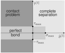
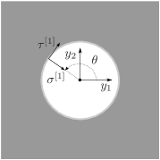
Figure 2. Interfacial constitutive law; (a) three-state model, (b) local coordinate system.

The set of admissible tractions then specializes to

$$\Lambda=\left\{\left(\widehat{\sigma}^{[1]}(\boldsymbol{y})\leq\sigma_{\max}\cap|\widehat{\tau}^{[1]}(\boldsymbol{y})|\leq\tau_{\max}\right)\cup\left(\widehat{\sigma}^{[1]}(\boldsymbol{y})\leq 0\right)\ \forall\boldsymbol{y}\in\Gamma^{[1]}\right\}.$$ (59)

Correspondingly, the constraint $\widehat{\boldsymbol{\lambda}}\in\Lambda$ is simply enforced by setting the traction value to zero whenever the corresponding strength is exceeded by the predicted value $\tilde{\boldsymbol{\lambda}}$. Note that it follows from duality theory that the condition $\widehat{\sigma}^{[1]}\leq 0$ is equivalent to the non-interpenetration for the matrix and fibers ($u_{n}^{[j]}\geq u_{n}^{[1]}$), cf. [11].

3.3. Implementation strategy

The resulting incremental algorithm compatible with the adopted interfacial law (59), inspired by a related study [46], is briefly summarized by means of a pseudo-code shown in Table 1. Note that in order to simplify the exposition, a proportional loading path in the form

$$\boldsymbol{E}(t)=t\boldsymbol{E}_{\max} 0\leq t\leq 1$$ with (60)

is considered. Moreover, the irreversibility of debonding is enforced using the static condensation [5, Section 2.5] of the corresponding entries of $\boldsymbol{d}_{\lambda}^{[1]}$, cf. lines 8 and 12 of Table 1.

i	Initialize material parameters (phase elastic properties) and geometry (mesh)
	assemble stiffness matrices $\mathbf{K}^{(i)}$,	Eqs. (51)
	transformation matrices $\mathbf{T}^{(i)}$ and compatibility matrices $\mathcal{E}^{(i)}$	Eqs. (53,54)
ii	Initialize loading data: macroscopic strain $\boldsymbol{E}_{\max}$
	assemble load vectors $\boldsymbol{f}_{\max}^{(i)}$	Eqs. (52)
iii	Computation FETI-based quantities:
	pseudoinverse $\mathbf{K}^{(i)}{{}^{\dagger}}$ and rigid body $\mathbf{R}^{(i)}$ matrices
iv	Setup interfacial strengths and pseudo-times $t_{1}<t_{2}<\ldots<t_{N}$
1	for $k=1:N$ (cycle through time steps)
2	set $\boldsymbol{f}^{(i)}=t_{k}\boldsymbol{f}_{\max}^{(i)}$ and $\boldsymbol{E}=t_{k}\boldsymbol{E}_{\max}$
3	do (outer loop)
4	predict distribution of interfacial tractions $\tilde{\boldsymbol{d}_{\lambda}}^{[1]}$ using MCG	Eqs. (57,55)
5	for $n=1:M$ (internal cycle though interfacial nodes)
6	extract $\tilde{\sigma}$ and $\tilde{\tau}$ for $n$-th node
7	if $\tilde{\sigma}\leq 0$ and $|\tilde{\tau}|\geq\tau_{\max}$ (contact problem)
8	set $\sigma=\tilde{\sigma}$ and $\tau=0$ by static condensation of $\mathcal{E}^{(i)}$ (without possibility of ”healing”)
9	elseif $\tilde{\sigma}\leq\sigma_{\max}$ and $|\tilde{\tau}|\leq\tau_{\max}$ (perfect bond)
10	set $\sigma=\tilde{\sigma}$ and $\tau=\tilde{\tau}$
11	else (complete separation)
12	set $\sigma=0$ and $\tau=0$ by static condensation of $\mathcal{E}^{(i)}$ (without possibility of ”healing”)
13	endif
14	endfor
15	until interfacial conditions remain unchanged
16	endfor

Table 1. Conceptual implementation of FETI-based solver for debonding problem

4. Micromechanical model

In the current Section, a simplified micromechanics-based solution to the debonding problem is constructed, in order to, at the same time, verify the developed FETI-based algorithm as well as to assess the added value of the the detailed numerical modelling. To that end, a composite is treated as a two-phase material, consisting of a matrix phase (domain ${\Omega^{(1)}}$), occupied by $(n-1)$ indistinguishable particles (related to domains ${\Omega^{(2)}},{\Omega^{(3)}},\ldots,{\Omega^{(n)}}$ in the FETI-based method). Moreover, the available geometrical information is reduced to the phase volume fractions $c^{(1)}$ and $c^{(2)}$, defined as

$$c^{(1)}=\frac{{|{\Omega^{(1)}}|}}{{|{\Omega^{\mathcal{UC}}}|}}, c^{(2)}=1-c^{(1)},$$ (61)

where, in accord with the rest of the current section, a symbol $\bullet^{(1)}$ is reserved for a quantity related to the matrix phase while $\bullet^{(2)}$ collectively describes particle-related unknowns.

Employing the simplified data, the overall stiffness of a two-phase composite reads

$$\mathbf{L}^{\rm eff}=\mathbf{L}^{(1)}+c^{(2)}\left(\mathbf{L}^{(2)}-\mathbf{L}^{(1)}\right)\mathbf{A}^{(2)},$$ (62)

where $\mathbf{L}^{(1)}$ and $\mathbf{L}^{(2)}$ are the matrix and particle stiffnesses, respectively, and $\mathbf{A}^{(2)}$ stands for a strain concentration factor, relating a macroscopic strain $\boldsymbol{E}$ to the average strain in a particle. It follows from the Benveniste’s reformulation [4] of the original Mori-Tanaka method [28] that the strain concentration factor can be accurately approximated as

$$\mathbf{A}^{(2)}\approx\mathbf{A}_{{\rm MT}}^{(2)}=\mathbf{T}^{(2)}\left(c^{(1)}{\mathbf{I}}+c^{(2)}\mathbf{T}^{(2)}\right)^{-1},$$ (63)

with $\mathbf{T}^{(2)}$ denoting the partial strain concentration factor (with a physical meaning of the average strain in a particle due to prescribed average strain in the matrix), expressed in the form

$$\mathbf{T}^{(2)}=\left({\mathbf{I}}+\mathbf{P}^{(2)}\left(\mathbf{L}^{(2)}-\mathbf{L}^{(1)}\right)\right)^{-1}.$$ (64)

The term $\mathbf{P}^{(2)}$ appearing in Equation (64) is the Walpole matrix [44], related to a response of an isolated inclusion embedded in an infinite matrix phase, which, under the assumption of circular fibers, isotropic matrix and plane strain state, can be explicitly expressed as, cf. [44]:

$$\mathbf{P}^{(2)}=\frac{1+{\nu^{(1)}}}{8E^{(1)}\left({\nu^{(1)}}-1\right)}\left[\begin{array}[]{rrr}8{\nu^{(1)}}-5&1&0\\ 1&8{\nu^{(1)}}-5&0\\ 0&0&32{\nu^{(1)}}-24\end{array}\right],$$ (65)

where $E^{(1)}$ a ${\nu^{(1)}}$ are the Young modulus and the Poisson ratio of the matrix phase.

When assuming a phase-wise uniform distribution of mechanical fields within heterogeneities, the stress value in a particle can be estimated as

$$\boldsymbol{\sigma}^{(2)}(\boldsymbol{y})\approx\boldsymbol{\sigma}_{{\rm MT}}^{(2)}=\mathbf{L}^{(2)}\mathbf{A}_{{\rm MT}}^{(2)}\boldsymbol{E},$$ (66)

and, employing the equilibrium conditions (43), converted into the approximate value of boundary tractions at the particle/matrix interface

$${\boldsymbol{\lambda}^{[1]}}(\theta)\approx{\boldsymbol{\lambda}^{[1]}}_{{\rm MT}}(\theta)=\mathbf{\boldsymbol{\nu}}^{[1]}(\theta){\sf{}^{T}}\boldsymbol{\sigma}^{(2)},$$ (67)

where $\theta$ is an angle parameterizing a position on the interface introduced in Figure 2 and the stress-traction transformation matrix $\mathbf{\boldsymbol{\nu}}^{[1]}$ is expressed using Equation (22) with $\boldsymbol{n}=\boldsymbol{n}^{[1]}=\left[\begin{array}[]{cc}-\cos\theta&-\sin\theta\end{array}\right]{\sf{}^{T}}$. The algorithmic implementation of the micromechanics-based solver closely follows the procedure introduced by Table 1. The debonding mechanism is reduced to a two-state description, with one state describing an undamaged composite, whereas the second state corresponds to completely debonded particles. In particular, the perfect bonding at the matrix/particle interface is maintained until the normal or tangential tractions do not exceed the local strengths,

$$\sigma^{[1]}_{{\rm MT}}(\theta)\leq\sigma_{\max}\mbox{ and }|\tau^{[1]}_{{\rm MT}}(\theta)|\leq\tau_{\max}\mbox{ for all }0\leq\theta<2\pi,$$ (68)

where $\sigma^{[1]}_{{\rm MT}}$ and $\tau^{[1]}_{{\rm MT}}$ denote the normal and tangential tractions determined from (67) via relation (41) with $\boldsymbol{t}^{[1]}=\left[\begin{array}[]{cc}\sin\theta&-\cos\theta\end{array}\right]{\sf{}^{T}}$. If the previous condition is violated for at least one value of $\theta$ for a given level of macroscopic strain, we irreversibly set $\mathbf{L}^{(2)}=\mathbf{0}$.

5. Numerical examples

Performance assessment of the numerical homogenization and the micromechanics-based solvers will be performed on the basis of two PUCs representing cross-sections typical of unidirectional composites: a parametric hexagonal unit cell model analyzed in Section 5.1 and a twenty-particle unit cell treated in Section 5.2, which was obtained in [47] by a careful analysis of a graphite/polymer composite sample. All FETI-based examples presented bellow are determined using an in-house code derived from a Matlab implementation of finite element solver introduced in [1] with the DistMesh code, developed by Persson and Strang [31], used to generate finite element meshes. The material properties of individual phases and interface are taken from a related study [19] and appear in Table 2. The plane strain assumption is adopted to reduce the analysis to a two-dimensional cross-section and the displacement fields are discretized using constant strain triangular elements with the characteristic element/fiber diameter ratio approximately equal to $0.05$. In all reported numerical simulations, the following discretization of the time interval $[0,1]$ was considered. First, assuming perfectly bonded phases, the value $t^{*}$ related to the debonding onset was determined. Next, the post-peak branch $(t^{*},1]$ was uniformly sampled using $N$ equisized intervals. An interested reader is referred to [17] for additional implementation-related details.

Matrix
Young’s modulus, $E^{(1)}$	$1$ GPa
Poisson’s ratio, $\nu^{(1)}$	$0.4$
Inclusion
Young’s modulus, $E^{(2)}$	$150$ GPa
Poisson’s ratio, $\nu^{(2)}$	$0.3$
Interface
Normal strength, $\sigma_{\max}$	$0.02$ GPa
Tangential strength, $\tau_{\max}$	$0.02$ GPa

Table 2. Material data of composite system

5.1. Hexagonal packing of particles

As the first example, we consider a hexagonal PUC subject to a bi-axial tensile/compressive strain load characterized by $\boldsymbol{E}_{\max}=\left[\begin{array}[]{ccc}0.02&-0.02&0\end{array}\right]{\sf{}^{T}},$ recall Equation (60). Stress paths for the ${\rm MT}$ scheme correspond to a fine discretization of the overall time ($N=100$), whereas the value $N=10$ was adopted for the FETI-based algorithm. Note that the coarse time stepping of the latter approach is mainly related to a high sensitivity of the post peak branch to inevitable geometrical imperfections of the finite element mesh. As illustrated in Figure 3, taking $N=100$ leads to a non-symmetric debonding mode, resulting in a substantially different distribution of local fields and overall response than for the symmetric deformation mechanism. When the time discretization is set to $N=10$, on the other hand, the larger value of the overall strain increment suppresses the mesh-induced imperfections and the solution symmetry is maintained.

The resulting macroscopic stress-strain relations obtained by the MT and FETI-based approaches for the fiber volume fraction $c^{(2)}=50\%$ appear in Figure 4. For comparison, the ideal debonding mode, corresponding to sufficiently small time increment and perfectly symmetric mesh, is indicated by gray color.

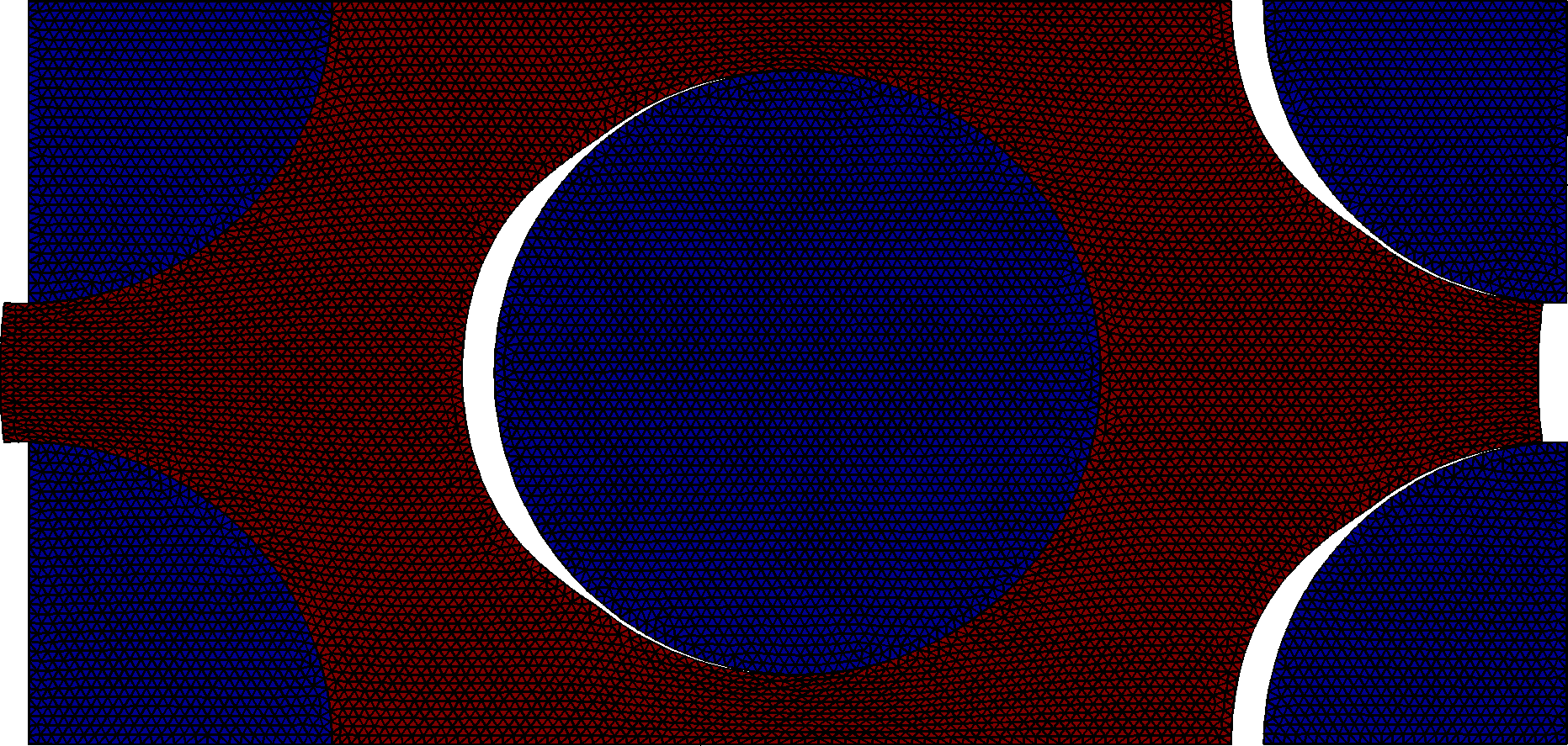
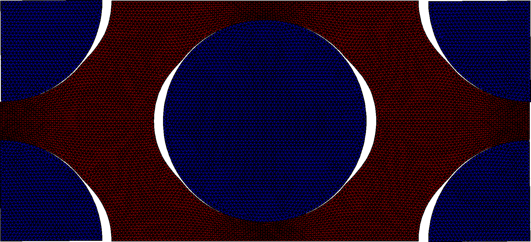
Figure 3. Scheme of debonding initiation for a hexagonal PUC; (a) $N=100$, (b) $N=10$. Displacements are scaled by factor of $20$.

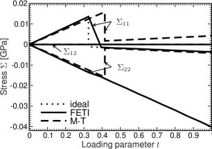
Figure 4. Macroscopic stress-strain diagram for hexagonal PUC; $c^{(2)}=50\%$.

In the elastic regime, both methods predict almost identical values of macroscopic stresses with the MT solver providing a slightly more compliant response than the FEM-based approach. Such behavior is consistent with the fact that the Mori-Tanaka estimates, for material systems with stiffer particles embedded in a weaker matrix phase, coincide with the lower Hashin-Shtrikman variational bounds, cf. [32]. A somewhat higher discrepancy is observed for the prediction of a debonding onset $t^{*}$, where the “unsafe” MT result yields $t^{*}_{{\rm MT}}\doteq 0.41$, which by about $25\%$ exceeds the reference value $t^{*}_{{\rm FETI}}\doteq 0.33$. The difference can be attributed to the value of constant fiber stress field adopted in the MT estimate. Such an assumption is well-justified when determining the mean response of a material with coherent interfaces, as demonstrated by excellent match of the elastic branches in Figure 4, but becomes less accurate when estimating the extreme stresses governing the failure process. This claim is further supported by plots of interfacial tractions at the debonding onset shown in Figure 5. We observe that, for the current case of $50\%$ particle volume fraction, the deviation of the fiber stress from the assumed uniformity in the MT method is further propagated to the values of local tractions. It is also worth noting that, up to some discretization-based effects, the FETI solution is free of spurious traction oscillations appearing when introducing interface elements between fibers and matrix as reported, e.g., in [37].

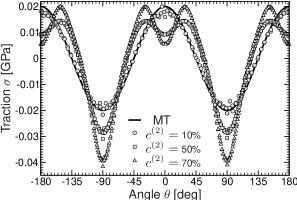
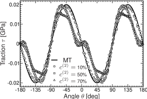
Figure 5. Distribution of interfactial tranctions at the onset of debonding; (a) normal and (b) tangential components; discrete values correspond to the FETI solution, the MT results are independent of $c^{(2)}$.

After the debonding initiation, the discrepancies between both approaches become even more pronounced. The MT solver predicts, due to the assumption of complete interfacial failure, a sudden drop of the stress values in both directions, reaching the values corresponding to an isotropic porous medium in the post-peak regime. The FETI-based model, being capable of capturing partial interfacial debonding, leads to a highly anisotropic mechanism: in the compressive direction, the response remains almost insensitive to the debonding phenomena, whereas the actual stress drop magnitude in the $y_{1}$ direction exceeds the value predicted by the MT scheme, leading eventually to the appearance of overall compressive stresses $\Sigma_{11}$ due to intra-phase contact. As these conclusions remain valid for both “ideal” and actual discretized stress paths, we will perform the assessment on the basis of the latter results in the sequel.

(a) FETI

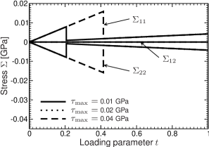
(b) MT

Figure 6. Influence of $\tau_{\max}$ for hexagonal PUC; $c^{(2)}=50\%$.

Next, we investigate the influence of $\tau_{\max}$ parameter on the overall behavior of the hexagonal unit cell, cf. Figure 6. It appears that, for the current test, the MT approach does not capture the change of failure mode when increasing the interfacial strength from $\tau_{\max}$ from $0.02$ to $0.04$ GPa. Such result can be again explained by inspecting traction distribution for $c^{(2)}=50\%$ shown in Figure 5. Due to the fact that $E_{11}=|E_{22}|$, the MT theory predicts identical extereme values of normal and shear tractions, which, in turn, implies that the debonding initiation is governed solely by the minimum value of $\sigma_{\max}$ and $\tau_{\max}$. The slight difference in the extreme shear and tensile tractions predicted by the FETI solver, on the other hand, leads to a three distict stress-strain curves, corresponding to a shear initiation for $\tau_{\max}=0.01$ GPa and $\tau_{\max}=0.02$ GPa, while for $\tau_{\max}=0.04$ GPa the debonding starts in the normal mode. Note that similar results are found when varying the $\sigma_{\max}$ parameter.

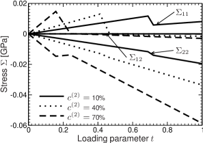
(a) FETI

(b) MT

Figure 7. Influence of volume fractions for hexagonal PUC.

The last aspect to be analyzed remains the particle volume fractions, cf. Figure 7. For the $\Sigma_{11}$ component, the results of the FETI-based solver predict a gradual transition of the debonding branch from tensile to compressive stress values with increasing particle volume fraction $c^{(2)}$. A closely related trend, resulting from stress redistribution due to intra-phase contact, is exhibited by the $\Sigma_{22}$ path, where the stress drop after debonding changes its sign with increasing $c^{(2)}$. The micromechanics-based solver, on the other hand, leads to a symmetric response in terms of normal macroscopic stresses with the difference in debonding time ranging from $7\%$ to $40\%$. This trend is in a perfect agreement with traction plots in Figure 5, demonstrating that the mismatch between traction distribution for the MT and FETI solvers generally increases for densely packed particles due to more complex interaction mechanism. In particular, for low volume fractions, the results of the analytical approach almost exactly duplicate the numerical data; the MT method, however, fails to reproduce the traction redistribution at increased particle volume fractions $c^{(2)}$.

5.2. Real-world microstructure

The universality of the conclusions reached for the hexagonal packing of particles is further supported by an analogous analysis of a twenty-fiber unit cell with particle volume fraction $c^{(2)}\doteq 43.9\%$, subject to a pure shear strain loading path with $\boldsymbol{E}_{\max}=\left[\begin{array}[]{ccc}0&0&0.02\sqrt{2}\end{array}\right]{\sf{}^{T}}$. The mutual comparison of macroscopic stress path appears in Figure 8, storing the results of the MT method and, to illustrate the effect of microstructural modeling, of the FETI solver for the disordered microstructure and the regular hexagonal packing with identical fiber volume fractions.

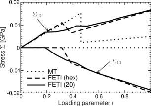
Figure 8. Macroscopic stress-strain response for 20-fiber PUC.

The stress paths predicted by FETI reflect somewhat different failure mechanisms for disordered and regular composite. In particular, the inelastic path for the $20$-fiber unit cell exhibits a piecewise linear evolution of the shear stresses, accompanied by a monotonically descreasing normal stresses. The observed deformation mechanism can be explained by the distribution of the local stress fields captured in Figure 9. In particular, the debonding onset is driven by stress amplification in the form of diagonal shear bands visible in Figure 9(a). After exceeding the interfacial strengths, see Figure 9(c), the concentrations are released at newly formed discontinuity interfaces, resulting in the formation of shifted shear bands connecting non-debonded particles and in local matrix-fiber contacts. Such mechanism is progressively repeated until the fully debonded state is reached, cf. Figure 9(e). For the regular microstructure, the debonding initiates simultaneously at all fibers and the stiffness immediately reaches the residual value (Figs. 9(b), 9(d) and 9(d)). It is worth noting that even the debonded composites we observed (up to minor discretization-induced effects) the stress values $\Sigma_{11}=\Sigma_{22}$, which confirms the spatial isotropy of the samples in question.

The proposed simple MT-based solution, on the other hand, shows a more compliant residual stiffness in the shear mode and predicts appearance zero normal stresses. Such response is again a direct consequence of the “porous” approximation adopted in the post-peak regime. Finally observe that the debonding onset pseudo-times, as predicted by different simulations, verify

$$t^{*}_{{\rm FETI}(20)}\doteq 0.19<t^{*}_{{\rm FETI}(\mathrm{hex})}\doteq 0.32<t^{*}_{{\rm MT}}\doteq 0.46,$$

cf. Figure 8, eventually demonstrating that the differences between the regular and irregular microstructures due to local stress amplicifactions can be well comparable with the value found when comparing the analytical approach to the detailed numerical model.

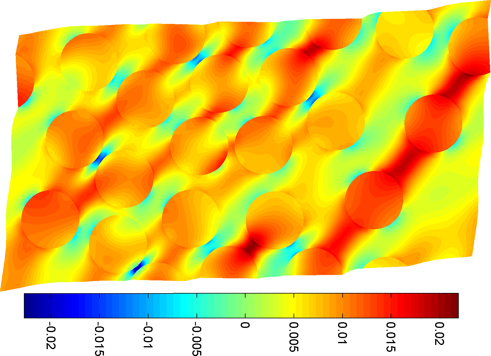
(a) $t\doteq 0.19$ (displacements are scaled by factor of $20$)

(b) $t\doteq 0.32$ (displacements are scaled by factor of $20$)

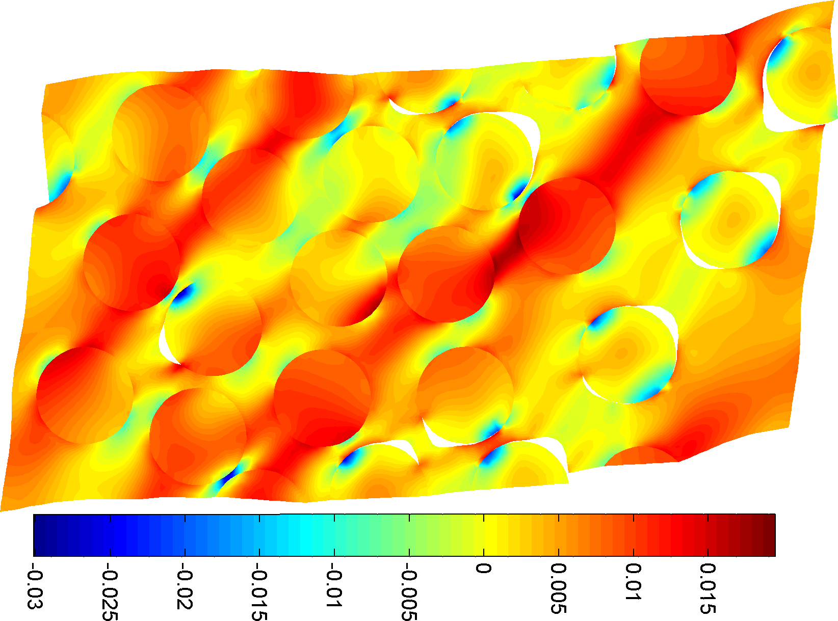
(c) $t\doteq 0.27$ (displacements are scaled by factor of $20$)

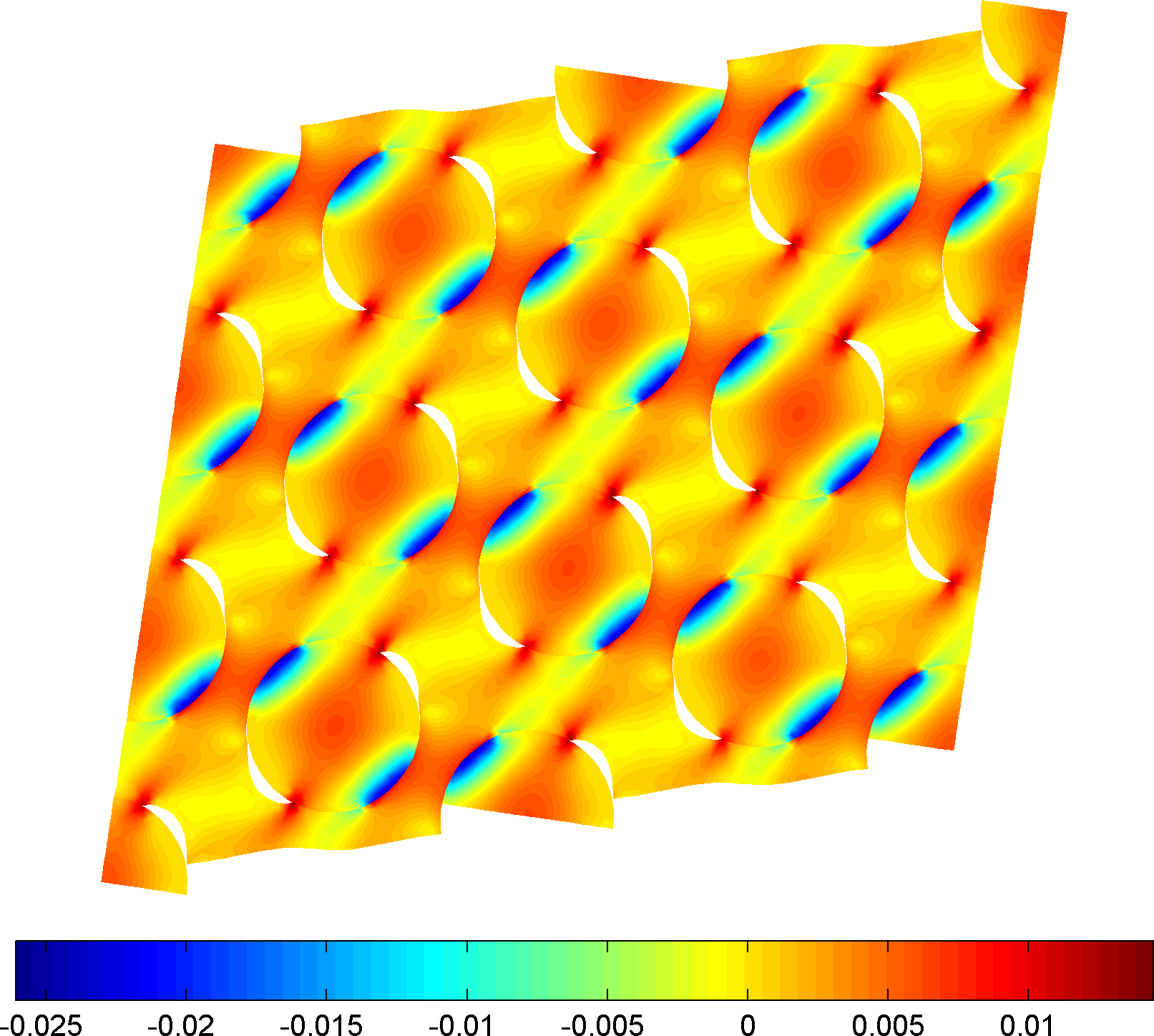
(d) $t\doteq 0.39$ (displacements are scaled by factor of $20$)

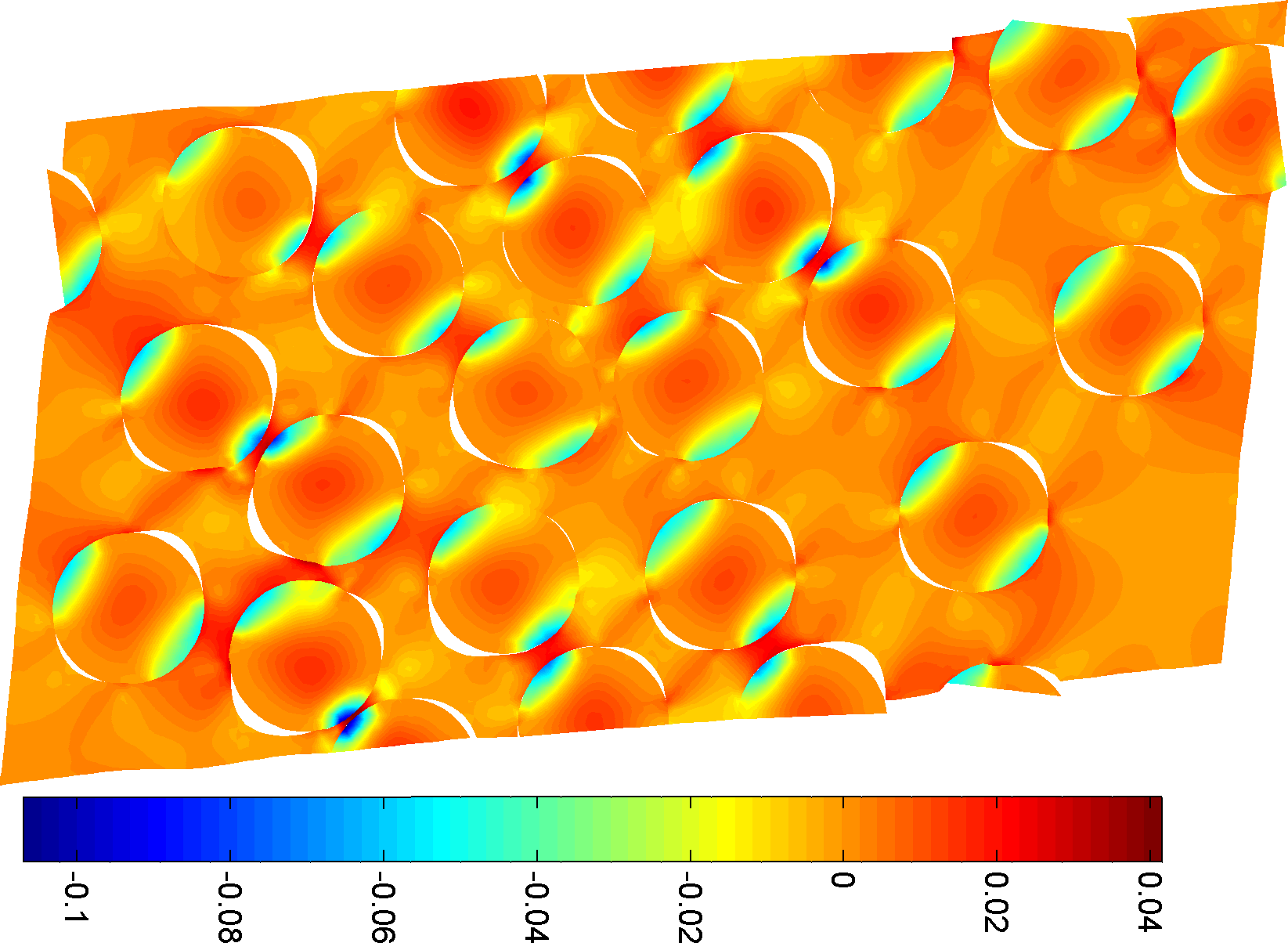
(e) $t=1$ (displacements are scaled by factor of $5$)

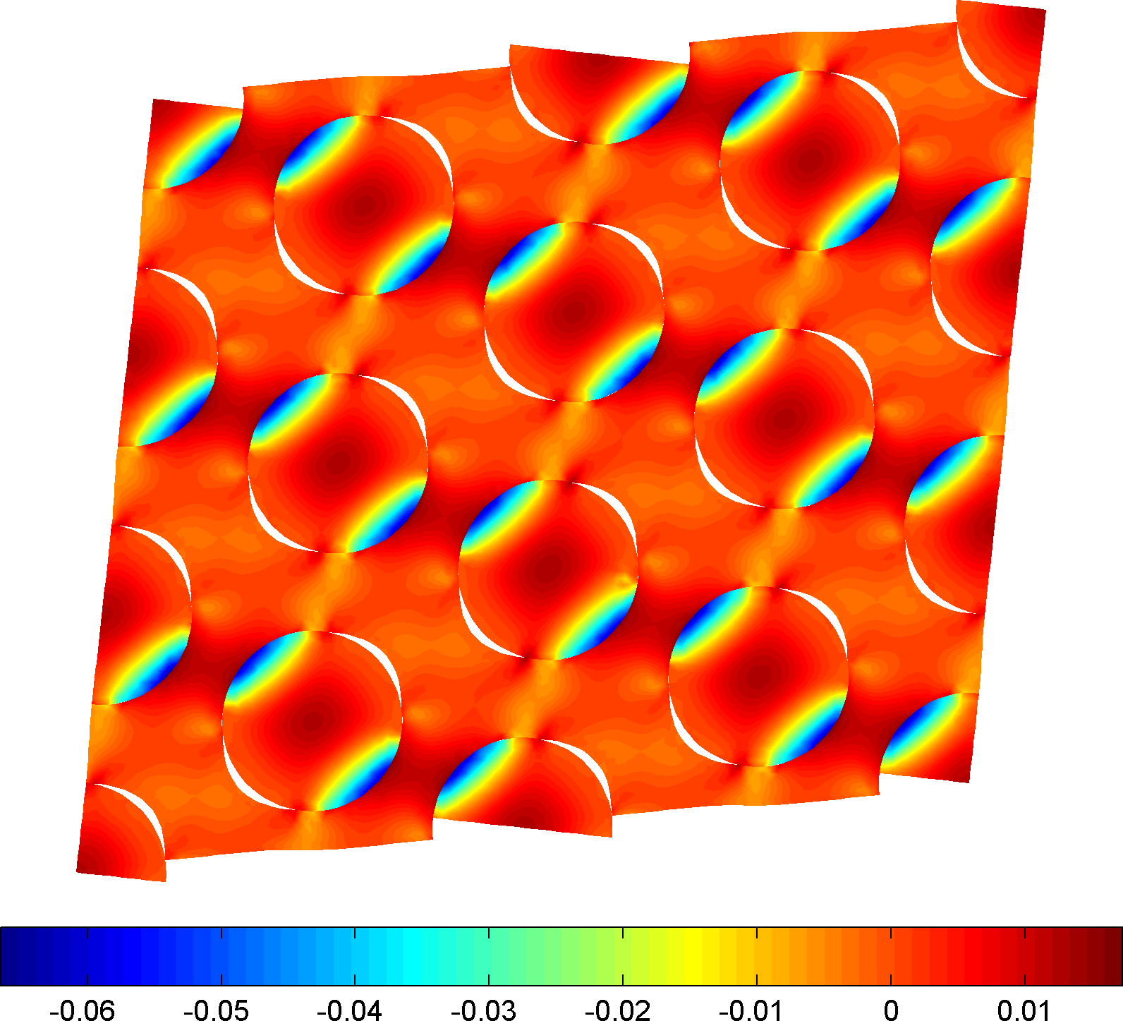
(f) $t=1$ (displacements are scaled by factor of $5$)

Figure 9. Distribution of maximum principal stress for a 20-fiber and equivalent hexagonal PUCs. The values are given in GPa.

6. Conclusions

In the current work, an overview of the FETI-based procedure for the homogenization of debonding composites was presented. In addition, the developed algorithm was used to perform a detailed assessment of a simplified micromechanics-based solver based on the MT method. The results of the performed studies have led to the following conclusions:

• The duality-based solver offers very promising approach to the homogenization of debonding composites, both from the point of view of numerical efficiency as well as the direct treatment of traction-based interfacial constitutive laws.

• The simple micromechanics-based solver is fully capable of accurate prediction of the elastic part of the loading branch. The onset of debonding process is captured with the difference from the numerical results ranging from approximately $10\%$ to $40\%$ for regular packing of particles.

• The assumption of completely debonded interfaces adopted in the MT solver, on the other hand, appear to be quite unrealistic and is mainly responsible for the inconsistent predictions in the post-peak regime.

• The results presented in Section 5.2 clearly confirm that the apparent post-critical response is influenced not only by details of particle arrangement, but also by the PUC size, cf. [43]. When dealing with inherently random real world composites, the choice of an appropriate statistically equivalent PUC becomes rather delicate and generally requires a proper statistical characterization in terms of geometry and mechanical quantities of interest, see [20, 48] for additional discussion.

The future extension of the FETI-based solver would involve a treatment of more realistic interfacial constitutive laws. For the micromechanics-based solver, the essential feature to incorporate seems to be the debonding-induced anisotropy in composite including the effect of contact stresses. Both topics enjoy our current interest and will be reported on separately.

References

- [1] J. Alberty, C. Carstensen, S. A. Funken, and R. Klose, MATLAB implementation of the finite element method in elasticity, Computing 69 (2002), no. 3, 239–263.
- [2] P. M. A. Areias and T. Rabczuk, Quasi-static crack propagation in plane and plate structures using set-valued traction-separation laws, International Journal for Numerical Methods in Engineering 74 (2008), no. 3, 475–505.
- [3] Y. Benveniste, The effective mechanical behaviour of composite materials with imperfect contact between the constituents, Mechanics of Materials 4 (1985), no. 2, 197–208.
- [4] Y. Benveniste, A new approach to the application of Mori-Tanaka theory in composite materials, Mechanics of Materials 6 (1987), no. 2, 147–157.
- [5] Z. Bittnar and J. Šejnoha, Numerical methods in structural mechanics, ASCE Press and Thomas Telford, Ltd, New York and London, 1996.
- [6] M.K. Chati and A.K. Mitra, Prediction of elastic properties of fiber-reinforced unidirectional composites, Engineering Analysis With Boundary Elements 21 (1998), no. 3, 235–244.
- [7] B. Cox and Q. Yang, In quest of virtual tests for structural composites, Science 314 (2006), no. 5802, 1102–1107.
- [8] C. Döbert, R. Mahnken, and E. Stein, Numerical simulation of interface debonding with a combined damage/friction constitutive model, Computational Mechanics 25 (2000), no. 5, 456–467.
- [9] Z. Dong and A. J. Levy, Mean field estimates of the response of fiber composites with nonlinear interface, Mechanics of Materials 32 (2000), no. 12, 739–767.
- [10] Z. Dostál, Optimal quadratic programming algorithms with applications to variational inequalities, Springer Optimization and Its Applications, vol. 23, Springer Verlag, New York, NY, USA, 2009.
- [11] Z. Dostál, D. Horák, and O. Vlach, FETI-based algorithms for modelling of fibrous composite materials with debonding, Mathematics and Computers in Simulation 76 (2007), no. 1–3, 57–64.
- [12] C. Farhat, J. Mandel, and F. X. Roux, Optimal convergence properties of the FETI domain decomposition method, Computer Methods in Applied Mechanics and Engineering 115 (1994), 365–385.
- [13] C. Farhat and F.-X. Roux, A method of finite element tearing and interconnecting and its parallel solution algorithm, International Journal for Numerical Methods in Engineering 32 (1991), no. 6, 1205–1227.
- [14] F. Feyel and J.-L. Chaboche, FE2 multiscale approach for modelling the elastoviscoplastic behaviour of long fibre SiC/Ti composite materials, Computer Methods in Applied Mechanics and Engineering 183 (2000), no. 3–4, 309–330.
- [15] M. Gosz, B. Moran, and J. D. Achenbach, On the role of interphases in the transverse failure of fiber composites, International Journal of Damage Mechanics 3 (1994), no. 4, 357–377.
- [16] P. Gruber, FETI-based homogenization of composites with perfect bonding and debonding of constituents, Bulletin of Applied Mechanics 4 (2008), no. 13, 11–17.
-
[17]
P. Gruber, Homogenization of composite materials with imperfect bonding of
constituents, Master’s thesis, Czech Technical University in Prague, 2008,
(in
Czech)
http://mech.fsv.cvut.cz/~grubepav/download/gruber_master_thesis%.pdf, [January 27, 2009]. - [18] Z. Hashin, Thermoelastic properties of fiber composites with imperfect interface, Mechanics of Materials 8 (1990), no. 4, 333–348.
- [19] H. M. Inglis, P. H. Geubelle, K. Matouš, H. Tan, and Y. Huang, Cohesive modeling of dewetting in particulate composites: Micromechanics vs. multiscale finite element analysis, Mechanics of Materials 39 (2007), no. 6, 580–595.
- [20] T. Kanit, S. Forest, I. Galliet, V. Mounoury, and D. Jeulin, Determination of the size of the representative volume element for random composites: statistical and numerical approach, International Journal of Solids and Structures 40 (2003), no. 13–14, 3647–3679.
- [21] V. Kouznetsova, W. A. M. Brekelmans, and P. T. Baaijens, An approach to micro-macro modeling of heterogeneous materials, Computational Mechanics 27 (2001), no. 1, 37–48.
- [22] J. Kruis, Domain decomposition methods for distributed computing, Saxe-Coburg Publications, Kippen, Stirling, Scotland, 2006.
- [23] J. Kruis and Z. Bittnar, Reinforcement-matrix interaction modeled by FETI method, Domain Decomposition Methods in Science and Engineering XVII (U. Langer, M. Discacciati, D. E. Keyes, O. B. Widlund, and W. Zulehner, eds.), Lecture Notes in Computational Science and Engineering, vol. 60, Springer Verlag, 2008, pp. 567–573.
- [24] S. Li and S. Ghosh, Debonding in composite microstructures with morphological variations, International Journal of Computational Methods 1 (2004), no. 1, 121–149.
- [25] K. Matouš, H. M. Inglis, X. Gu, D. Rypl, T. L. Jackson, and P. H. Geubelle, Multiscale modeling of solid propellants: From particle packing to failure, Composites Science and Technology 67 (2007), no. 7–8, 1694–1708.
- [26] J. C. Michel, H. Moulinec, and P. Suquet, Effective properties of composite materials with periodic microstructure: A computational approach, Computer Methods in Applied Mechanics and Engineering 172 (1999), no. 1–4, 109–143.
- [27] G. W. Milton, The theory of composites, Cambridge Monographs on Applied and Computational Mathematics, vol. 6, Cambridge University Press, 2002.
- [28] T. Mori and K. Tanaka, Average stress in matrix and average elastic energy of elastic materials with misfitting inclusions, Acta Metallurgica 21 (1973), no. 5, 571–573.
- [29] N. J. Pagano and G. P. Tandon, Modeling of imperfect bonding in fiber reinforced brittle matrix composites, Mechanics of Materials 9 (1990), no. 1, 49–64.
- [30] S. S. Pendhari, T. Kant, and Y. M. Desai, Application of polymer composites in civil construction: A general review, Composite Structures 84 (2008), no. 2, 114–124.
- [31] P.-O. Persson and G. Strang, A simple mesh generator in MATLAB, SIAM Review 46 (2004), no. 2, 329–345.
- [32] P. Ponte Castañeda and J.R. Willis, The effect of spatial distribution on the effective behaviour of composite materials and cracked media, Journal of the Mechanics and Physics of Solids 43 (1995), no. 12, 1919–1951.
- [33] P. Procházka, Homogenization of linear and of debonding composites using the BEM, Engineering Analysis with Boundary Elements 25 (2001), no. 9, 753–769.
- [34] P. Procházka and M. Šejnoha, Development of debond region of lag model, Computers & Structures 55 (1995), no. 2, 249–260.
- [35] A. Rekik, F. Auslender, M. Bornert, and A. Zaoui, Objective evaluation of linearization procedures in nonlinear homogenization: A methodology and some implications on the accuracy of micromechanical schemes, International Journal of Solids and Structures 44 (2007), no. 10, 3468–3496.
- [36] K. Rektorys, Variational methods in mathematics, science and engineering, second ed., Springer Verlag, 2007.
- [37] J. C. J. Schellekens and R. De Borst, On the numerical integration of interface elements, International Journal for Numerical Methods in Engineering 36 (1993), no. 1, 43–66.
- [38] H. Tan, Y. Huang, C. Liu, and P. H. Geubelle, The Mori-Tanaka method for composite materials with nonlinear interface debonding, International Journal of Plasticity 21 (2005), no. 10, 1890–1918.
- [39] G. P. Tandon and N. J. Pagano, Effective thermoelastic moduli of a unidirectional fiber composite containing interfacial arc microcracks, Journal of Applied Mechanics 63 (1996), no. 1, 210–217.
- [40] H. Teng, Transverse stiffness properties of unidirectional fiber composites containing debonded fibers, Composites Part A: Applied Science and Manufacturing 38 (2007), no. 3, 682–690.
-
[41]
O. Vlach, Modelling of composites using duality-based solvers, Master’s
thesis, Technical University of Ostrava, 2001, (in Czech)
http://dspace.vsb.cz/handle/10084/41719, [January 27, 2009]. - [42] M. Šejnoha and M. Srinivas, Modeling of effective properties of composites with interfacial microcracks using PHA model, Building Research Journal 46 (1998), no. 2, 99–108.
- [43] M. Šejnoha, R. Valenta, and J. Zeman, Nonlinear viscoelastic analysis of statistically homogeneous random composites, International Journal for Multiscale Computational Engineering 2 (2004), no. 4, 644–672.
- [44] L. J. Walpole, On the overall elastic moduli of composite materials, Journal of the Mechanics and Physics of Solids 17 (1969), no. 4, 235–251.
- [45] M. E. Walter, G. Ravichandran, and M. Ortiz, Computational modeling of damage evolution in unidirectional fiber reinforced ceramic matrix composites, Computational Mechanics 20 (1997), no. 1, 192–198.
- [46] P. Wriggers, G. Zavarise, and T. I. Zohdi, A computational study of interfacial debonding damage in fibrous composite materials, Computational Materials Science 12 (1998), no. 1, 39–56.
- [47] J. Zeman and M. Šejnoha, Numerical evaluation of effective elastic properties of graphite fiber tow impregnated by polymer matrix, Journal of the Mechanics and Physics of Solids 49 (2001), no. 1, 69–90.
- [48] J. Zeman and M. Šejnoha, From random microstructures to representative volume elements, Modelling and Simulation in Materials Science and Engineering 15 (2007), no. 4, S325–S335.
Acknowledgements
Financial support of this work provided by the Grant Agency of the Czech Republic, project no. GAČR 106/08/1379, is gratefully acknowledged.