Odd-Even Crossover in a non-Abelian $\nu=5/2$ Interferometer

Abstract

We compute the backscattered current in a double point-contact geometry of a Quantum Hall system at filling fraction $\nu=5/2$ as a function of bias voltage in the weak backscattering regime. We assume that the system is in the universality class of either the Pfaffian or anti-Pfaffian state. When the number of charge $e/4$ quasiparticles in the interferometer is odd, there is no interference pattern with period $4\Phi_{0}$ at temperatures and source-drain voltages high enough that the coupling between bulk quasiparticles and the edge can be neglected. However, the coupling between a bulk charge $e/4$ quasiparticle and the edge causes it to be effectively absorbed by the edge at low temperatures and voltages. Consequently, even with an odd number of $e/4$ quasiparticles in the interferometer, an interference pattern with period $4\Phi_{0}$ appears at low bias voltages and temperatures, as if there were an even number of quasiparticles in the interferometer. We relate this problem to that of a semi-infinite Ising model with a boundary magnetic field. Using the methods of perturbed boundary conformal field theory, we give an exact expression for this crossover of the interferometer as a function of bias voltage. Finally, we comment on the possible relevance of our results to recent interference experiments.

I Introduction

A two point-contact interferometer Chamon97 ; Fradkin98 ; Camino05 is potentially a valuable probe of the topological properties of quantum Hall states. If the observed state at $\nu=5/2$ Willett87 ; Eisenstein02 ; Xia04 were non-Abelian Moore91 ; Nayak96c ; Ivanov01 , there would be a very dramatic signature in transport through a two point-contact interferometer Bonderson06a ; Stern06 ; Overbosch07 ; Bishara08 . If there is an even number of charge $e/4$ quasiparticles in the interferometer, then Aharonov-Bohm oscillations of the current are observed as the area of the loop is varied, due to the interference between the two possible tunneling paths for current-carrying charge $e/4$ quasiparticles. If there is an odd number of quasiparticles in the loop, then these Aharonov-Bohm oscillations are not observed as a result of the non-Abelian braiding of the current-carrying $e/4$ quasiparticles with those in the bulk. (However, Aharonov-Bohm oscillations with twice the period will still be observed due to the current carried by charge $e/2$ quasiparticles Bishara09 .) A recent experiment Willett09 may have observed this predicted effect.

In this experiment, a side gate is used to vary the area of the quantum Hall droplet in the interferometer. The current oscillates as the area is varied. However, at certain values of the side gate voltage, the interference pattern changes dramatically. According to the non-Abelian interferometry interpretation, such a change occurs when the area is varied beyond a point at which one of the quasiparticles leaves the interference loop. Then the $e/4$ quasiparticle number parity in the interference loop changes, leading to a striking change in the interference pattern. Close to a transition point in the $e/4$ quasiparticle number parity, a quasiparticle comes close to the edge of the quantum Hall droplet and begins to interact with the edge excitations. The leading coupling of the $e/4$ quasiparticle to the edge is through the (resonant) tunneling of Majorana fermions from the edge to the zero mode on the $e/4$ quasiparticle. This coupling makes it possible for $e/4$ Aharonov-Bohm oscillations to be seen even when there is an odd number of quasiparticles in the interference loop. At an intuitive level, this can be understood in the following way. For odd quasiparticle number, a topological qubit straddles one of the point contacts and records when an $e/4$ quasiparticle takes that path; consequently the two paths do not interfere and Aharonov-Bohm oscillations are not seen. This qubit is flipped when a Majorana fermion tunnels from the edge to a bulk zero mode in the interference loop, thereby erasing the record and allowing quantum interference. Over longer time scales, the topological qubit flips so many times that it can no longer carry any information. This eventually leads, at low energies and long time scales, to the absorption of the zero mode by the edge and, therefore, to the effective removal of this quasiparticle from the interference loop, as far as its non-Abelian braiding properties are concerned. Thus, every bulk quasiparticle will appear to be effectively absorbed by the edge if the interferometer is probed at sufficiently low voltages and temperatures – but ‘sufficiently low’ will be exponentially small in the distance of the quasiparticle from the edge, as we will see. Thus, the effect of bulk-edge coupling will only be apparent when the edge is close to a bulk $e/4$ quasiparticle. In this paper, we analyze this coupling in detail, as it effects the behavior of a two point-contact interferometer, with possible relevance to the transition regions of the experiments of Refs Willett09, .

In Ref. Fendley09, , the coupling of a bulk $e/4$ quasiparticle to the edge was formulated in terms of perturbed boundary conformal field theory. It was shown that this problem could be mapped to a semi-infinite Ising model in a boundary magnetic field. As we discuss below, the absence of $e/4$ quasiparticle interference for an odd number of bulk quasiparticles corresponds to the vanishing of the one-point function $\langle\sigma(x)\rangle=0$ when the boundary magnetic field vanishes, while the appearance of $e/4$ quasiparticle interference for an even number of bulk quasiparticles corresponds to $\langle\sigma(x)\rangle=x^{-1/8}$ when the boundary magnetic field is infinite ($x$ is the distance to the boundary of the Ising model which is assumed, for simplicity, to be the $y$-axis). For finite boundary magnetic field, the boundary conditions of the Ising model cross over from free to fixed, which corresponds to the absorption of a bulk quasiparticle. Following the derivation of of the exact crossover function for the magnetization by Chatterjee and Zamolodchikov Chatterjee94 (and of the full boundary state by Chatterjee Chatterjee95 ), we compute the current through the interferometer to lowest order in the backscattering at the point contacts, but treating the bulk-edge coupling exactly. Our results agree with lowest order perturbation theory in the bulk-edge coupling Overbosch07 and numerical solution of a lattice model Rosenow07b . When the point contacts are close together compared to ${v_{n}}/{e^{*}}V$, where $v_{n}$ is the Majorana fermion edge velocity, ${e^{*}}=e/4$, and $V$ is the source-drain voltage, the current-voltage relation takes a particularly simple form. When there is an even number of quasiparticles in the bulk, one of which is close to the edge, an interesting non-equilibrium problem presents itself: suppose the internal topological state of the bulk quasiparticles is fixed to an initial value; what is its subsequent time evolution. This is considered elsewhere.

II Model

We now set up the calculation of the backscattered current in a two point-contact interferometer to lowest order. The Pfaffian and anti-Pfaffian cases are conceptually similar, so we focus on the Pfaffian for the sake of concreteness. The edge theory of the Pfaffian state has a chiral bosonic charge mode and a chiral neutral Majorana modeMilovanovic96 ; Bena06 ; Fendley06 ; Fendley07a

$${\cal L}^{R}_{\rm Pf}(\psi,\phi)=\frac{2}{4\pi}\partial_{x}\phi\left(\partial_{t}+v_{c}\partial_{x}\right)\phi+i\psi\left(\partial_{t}+iv_{n}\partial_{x}\right)\psi$$ (1)

Both modes propagate to the right (the left-moving version of this action, ${\cal L}^{R}_{\rm Pf}$, has time-derivative terms with opposite sign), but will have different velocities in general. The velocities of the charged and neutral modes are $v_{c}$ and $v_{n}$, respectively. Recent numerical calculations and experiments indicate that ${v_{c}}\sim 10^{5}$ m/s, while ${v_{n}}\sim{v_{c}}/10$ (see, for instance, Ref. Wan06, ; Zhang09, ). The electron operator and $e/4$ quasiparticle operators are, respectively, $\Phi_{el}=\psi e^{i\sqrt{2}\phi}$ and $\Phi_{1/4}=\sigma e^{i\phi/2\sqrt{2}}$, where $\sigma$ is the Ising spin field of the Majorana fermion theoryFendley07a .

In the interferometer geometry depicted in Fig. 1, the edge modes are oppositely directed on the bottom and top edges, which we done by the subscripts $1,2$. The two point contacts are at $x_{a}$, $x_{b}$, and the corresponding $e/4$ quasiparticle backscattering amplitudes are $\Gamma_{a}$, $\Gamma_{b}$. Experimental values Willett09 ; Zhang09 of $|{x_{a}}-{x_{b}}|$ can range from approximately $1\mu$m to $5\mu$m, while ${|\Gamma_{a,b}|^{2}}\sim 0.1$. In the absence of backscattering at the point contacts or bulk-edge coupling, the action of the device is:

$${S_{0}}=\int dt\int dx\,\left({\cal L}^{R}_{\rm Pf}({\psi_{1}},{\phi_{1}})+{\cal L}^{L}_{\rm Pf}({\psi_{2}},{\phi_{2}})\right)$$ (2)

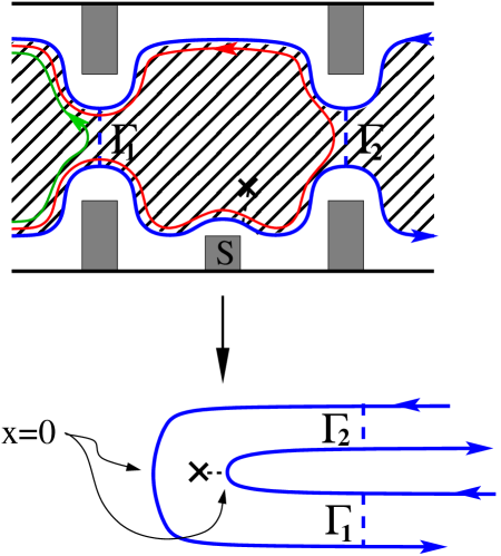
Figure 1: A double point-contact interferometer. Edge quasiparticles tunnel at two point-contacts with amplitudes $\Gamma_{1}$ and $\Gamma_{2}$, respectively. The interferometry area is changed by applying a voltage to gate $S$. A bulk quasiparticle is coupled to the bottom edge by Majorana fermion tunneling. This setup can be reformulated as two semi-infinite non-chiral edges or, equivalently, two semi-infinite Ising models. One Ising model has fixed boundary condition; the other had free boundary condition and a boundary magnetic field.

When inter-edge backscattering is weak, we expect the amplitude $\Gamma$ for charge-$e/4$ to be transferred from one edge to the other to be larger than for higher charges $ne/4$ Bishara09 . It is also the most relevant backscattering operator in the Renormalization Group sense Fendley06 ; Fendley07a , so we will focus on it. Since it is relevant, its effective value grows as the temperature is decreased, eventually leaving the weak backscattering regime. We assume that the temperature or voltage is high enough that the system is still in the weak inter-edge backscattering regime and a perturbative calculation is valid, but still much lower than the bulk energy gap. Following Refs. Chamon97, ; Bishara08, , inter-edge backscattering leads to a term of the form

$$S_{\text{backscatt}}=\int dt\,\,\bigl{(}{\Gamma_{a}}e^{-i{\omega_{J}}t}\,\,{T_{a}}(t)\>+\>\text{c.c.}\>+\\ {\Gamma_{b}}\,e^{2\pi i(\frac{\Phi}{4\Phi_{0}}-\frac{{n_{q}}}{8}+\frac{n_{\psi}}{2})}\>e^{-i{\omega_{J}}t}\,\,{T_{b}}(t)\>+\>\text{c.c.}\bigr{)}$$ (3)

where

$$T_{a}(t)={\sigma_{1}}(x_{a},t)\,{\sigma_{2}}(x_{a},t)\,\,e^{\frac{i}{\sqrt{8}}\left({\phi_{1}}(x_{a},t)-{\phi_{2}}(x_{a},t)\right)}$$ (4)

and similarly for ${T_{b}}(t)$. The Josephson frequency for a charge $e/4$ quasiparticle with voltage $V$ applied between the bottom and top edges is $\omega_{J}={e^{*}}V=\frac{eV}{4}$ (in units in which $\hbar=1$). The difference in the magnetic fluxes enclosed by the two trajectories around the interferometer is $\Phi$. We have chosen a gauge in which the vector potential is concentrated at the second point contact so that $\Phi$ enters only through the second term above. $n_{q}$ is the total electrical charge of the bulk quasiparticles, in units of $e/4$; ${n_{\psi}}=0,1$ is the Majorana fermion number in the interference loop, modulo $2$. The $n_{q}$ and $n_{\psi}$ terms in $\Gamma_{b}$ account for the diagonal (in the fermion number basis) effects of quasiparticle statistics. The product of right- and left-moving spin fields in (4) must be handled with some care to account for the fact that two charge $e/4$ quasiparticles (one on each edge) can fuse in two different ways. The effect of the non-Abelian braiding statistics of the bulk quasiparticles enters in this way through the precise definition of $T_{a,b}$. Fortunately, this can be handled in a simple way in a calculation to lowest-order in the backscattering operator, as we will see in the next section.

We now consider the coupling between a bulk quasiparticle and the edge. Suppose that one of the bulk quasiparticles is close to the bottom edge, at $x=x_{0}$ with ${x_{a}}<{x_{0}}<{x_{b}}$, as depicted in Fig. 1. Each bulk $e/4$ quasiparticle has a Majorana fermion zero mode Read96 ; Read00 ; we will denote the zero mode associated with the $e/4$ quasiparticle close to the edge by $\psi_{0}$. Then, the leading coupling between the edge and this quasiparticle is of the form:

$$S_{\text{bulk-edge}}=\int dt\,\left({\psi_{0}}{\partial_{t}}{\psi_{0}}+2ih\,{\psi_{0}}\,{\psi_{1}}\!({x_{0}})\right)$$ (5)

Here, $2h$ is the amplitude for a Majorana fermion to tunnel from the edge to the zero mode $\psi_{0}$.

Thus, the total action for a two-point contact interferometer with one or more quasiparticles in the interference loop, one of which is close to the bottom edge, is of the form

$$S={S_{0}}+S_{\text{backscattering}}+S_{\text{bulk-edge}}$$ (6)

However, this description is, at the moment, incomplete because we have not precisely defined the product of Ising spin fields in $S_{\text{backscattering}}$. We will do this in the next section, but first we will give the appropriate Kubo formulae for current through the interferometer.

The current operator can be found from the commutator of the backscattering Hamiltonian and the charge on one edge:

$$I(t)=\frac{ie}{4}\left(\Gamma_{a}e^{-i\omega_{J}t}\,{T_{a}}(t)-\text{h.c.}\right)\\ +\frac{ie}{4}\left({\Gamma_{b}}\,e^{2\pi i(\frac{\Phi}{4\Phi_{0}}-\frac{{n_{q}}}{8}+\frac{n_{\psi}}{2})}\>e^{-i{\omega_{J}}t}\,{T_{b}}(t)-\text{h.c.}\right)$$ (7)

To lowest order in perturbation theory, the backscattered current is found to be:

$$\langle I(t)\rangle=-i\int_{-\infty}^{t}dt^{\prime}\,\langle 0|[I(t),H_{\text{backscatt}}(t^{\prime})]|0\rangle$$ (8)

In principle, the current must be computed using a non-equilibrium technique, such as the Schwinger-Keldysh method, when the voltage is finite. However, at first order in the backscattering operators, there is no difference between the Schwinger-Keldysh expression and (8).

At this order, the current naturally breaks into the sum of three terms $I=I_{a}+I_{b}+I_{\rm int}$ where

$$I_{a,b}=\frac{e}{4}\left|\Gamma_{a,b}\right|^{2}\,\int_{-\infty}^{0}\!\!dt\,e^{i{\omega_{J}}t}\bigl{(}\langle{T_{a,b}}(0){T_{a,b}^{\dagger}}(t)\rangle\\ -\langle{T_{a,b}^{\dagger}}(0){T_{a,b}}(t)\rangle\bigr{)}$$ (9)

are the backscattered currents for each point contact independently and, following Chamon et al.Chamon97 , we write the interference term in the form:

$$I_{\rm int} =\frac{e}{4}\,\Gamma_{a}\tilde{\Gamma}_{b}^{*}\,\int_{-\infty}^{0}\!\!dt\,e^{i{\omega_{J}}t}\bigl{(}\langle{T_{a}}(0){T_{b}^{\dagger}}(t)\rangle-\langle{T_{b}^{\dagger}}(0){T_{a}}(t)\rangle\bigr{)}$$ (10)

$$\hskip 19.91684pt+\>\text{c. c.}$$ (11)

$$=\frac{e}{4}\cdot 2\,\text{Re}\Bigl{(}\Gamma_{a}{\tilde{\Gamma}_{b}^{*}}\bigl{[}\tilde{P}({\omega_{J}})-\tilde{P}(-{\omega_{J}})\bigr{]}\Bigr{)}$$ (12)

where $\tilde{\Gamma}_{b}={\Gamma_{b}}\,e^{2\pi i(\frac{\Phi}{4\Phi_{0}}-\frac{{n_{q}}}{8}+\frac{n_{\psi}}{2})}$. and the imaginary part of the response function is

$$\tilde{P}({\omega_{J}})=\int_{-\infty}^{\infty}\!\!dt\,e^{i{\omega_{J}}t}\,\langle{T_{a}}(0){T_{b}^{\dagger}}(t)\rangle$$ (13)

$I_{\rm int}$ is due to interference between the process in which a quasiparticle tunnels between the two edges at $x_{a}$ and the process in which it continues to $x_{a}$ and tunnels there. As a result, $I_{\rm int}$ depends on the magnetic flux and the number of bulk quasiparticles between the two point contacts; it reflects the non-Abelian statistics of quasiparticles. This is implemented through the precise definition of the product of Ising spin fields which appears in the backscattering operators, to which we turn in the next section.

III Backscattering Operators and Interference

We now review the a few essential points in the discussion of inter-edge backscattering in Refs. Fendley06, ; Fendley07a, . In the chiral Ising model, a pair of $\sigma$s can fuse to either $1$ or $\psi$ (or any linear combination of the two). Consequently, when we consider the correlation function of a string of $2n$ (chiral) $\sigma$ fields at a single edge, there is not a unique answer but, instead, a vector space of $2^{n-1}$ conformal blocks which are defined by specifying the fusion channels of the $\sigma$s (e.g. by dividing them arbitrarily into $n$ pairs and specifying how each pair fuses; different pairings lead to different bases in the vector space).

When a charge $e/4$ quasiparticle backscatters from one edge to another, a pair of $\sigma$ quasiparticles is created, one in the non-Abelian sector of each edge (recall that a $\sigma$, which is the non-Abelian part of an $e/4$ quasiparticle, is its own anti-particle). When there is only a single point contact and all bulk quasiparticles are far from the point contact, we can take this pair of $\sigma$s to fuse to $1$ since the backscattering process is a very small motion of a quasiparticle which does not involve any braiding and, therefore, does not create a $\psi$. An alternative way to understand this is to note that one can choose a gauge in which the non-Abelian gauge field due to bulk quasiparticles vanishes at the point contact. In this way, we can give a precise meaning to operators such as $T_{a,b}$. However, when we compute perturbatively in the backscattering, we would like to know how successive $\sigma$ fields on the same edge fuse. Fortunately, the condition that the pair of $\sigma$s which is created on opposite edges by a backscattering event can be converted (using a feature of anyon systems called the $F$-matrix) into a condition on the fusion channels of successive $\sigma$ fields on the same edge. This leads, according to the arguments of Refs. Fendley06, ; Fendley07a, , to a mapping of the single point contact problem to a Kondo-esque impurity problem.

When there are two point contacts, the quasiparticle history associated with a backscattering process at one of the point contacts must necessarily wind around the bulk quasiparticles in the interferometer. Equivalently, the non-Abelian gauge field due to bulk quasiparticles is non-vanishing at one of the point contacts or along one of the edges between the two point contacts; the simplest gauge is one in which the gauge field is concentrated at one of the point contacts, say contact $b$. If there is an even number of quasiparticles in the interferometer, their effect can be encapsulated in an extra phase ${n_{\psi}}\pi$ (dependent on the overall parity of the topological qubits in the interference loop) which we have absorbed into $\Gamma_{b}$. However, as shown in Ref. Bishara08, , if there is an odd number of quasiparticles in the loop, then the pair of $\sigma$s which is created by $T_{b}$ must fuse to $\psi$ instead of $1$. This makes no difference as far as local properties of that point contact are concerned. (In fact, in the single point-contact problem, we could have taken each backscattered pair to fuse to $\psi$ instead of to $1$, which would correspond to a non-standard gauge choice. This would have no effect on any physical property and would lead to the same Kond-esque model.)

However, if we consider the interference between the backscattering processes due to $T_{a}$ and $T_{b}$ when there is an odd number of quasiparticles in the interference loop, it is significant that the pair of $\sigma$s created by the former fuse to $1$ but those created by the latter fuse to $\psi$. If we consider the current to lowest order in the backscattering, the interference term (10) contains the expression

$$\langle{T_{a}}(0){T_{b}^{\dagger}}(t)\rangle =\langle{\left[{\sigma_{1}}({x_{a}},0)\,{\sigma_{2}}({x_{a}},0)\right]_{1}}\,\,{\left[{\sigma_{1}}({x_{b}},t)\,{\sigma_{2}}({x_{b}},t)\right]_{\psi}}\rangle$$

$$=\langle{\left[{\sigma_{1}}({x_{a}},0)\,{\sigma_{1}}({x_{b}},t)\right]_{\psi}}\rangle\,\,\langle{\left[{\sigma_{2}}({x_{a}},0)\,{\sigma_{2}}({x_{b}},t)\right]_{1}}\rangle$$

$$\hskip 14.22636pt+\>1\leftrightarrow 2$$

Here, we have used square brackets to denote the fusion channels of pairs of $\sigma$ fields. The correlation function in the first line factorizes, as shown on the second line, because we are perturbing around the limit in which the edges are decoupled. This expression vanishes because $\langle{\left[{\sigma_{2}}({x_{a}},0)\,{\sigma_{2}}({x_{b}},t)\right]_{\psi}}\rangle$ vanishes by fermion number parity conservation. However, when a bulk quasiparticle is coupled to the edge according to (5), fermion number parity is no longer conserved. Thus, this correlation function need not vanish, and an interference term can be present even for odd quasiparticle numbers Overbosch07 ; Rosenow07b . For instance, to lowest order in the tunneling amplitude $h$ in (5), $\langle{T_{a}}(0){T_{b}^{\dagger}}(t)\rangle$ will contain a non-vanishing contribution of the form Overbosch07

$$h\langle\psi_{0}\rangle\,\langle{\psi_{1}}({x_{0}},t^{\prime})\,{\left[{\sigma_{1}}({x_{a}},0){\sigma_{1}}({x_{b}},t)\right]_{\psi}}\rangle\,\langle{\left[{\sigma_{2}}({x_{a}},0)\,{\sigma_{2}}({x_{b}},t)\right]_{1}}\rangle\,$$

As discussed in Ref. Overbosch07, , this leads to a non-vanishing interference term for odd quasiparticle numbers with different scaling properties (as a function of $T,V$) than for even quasiparticle numbers. In the next section, we show how this interference term can be computed exactly in $h$ (but still to lowest order in ${\Gamma_{a}}\tilde{\Gamma}_{b}^{*}$).

IV Mapping to the Ising Model with a Boundary

When there is an even number of $e/4$ quasiparticles in the bulk of a Pfaffian or anti-Pfaffian droplet, the Majorana fermions have anti-periodic boundary conditions. When there is an odd number, the Majorana fermions have periodic boundary conditions. This can be understood in terms of the classical critical $2D$ Ising model in the following wayFendley09 . The droplet is ‘squashed’ down so that the bottom and top edges become the right- and left-moving modes of the Ising model. The bulk is forgotten about, except insofar as it affects the boundary conditions at the two ends of the droplet, where right-moving modes are reflected into left-moving ones and vice versa. Since there is no scale in this problem, the boundary conditions must be conformally-invariant; in the Ising model, this means that the Ising spins can either have free or fixed boundary conditions. When there is an even number of quasiparticles in the bulk and their combined topological qubit has a fixed fermion number parity, there are fixed boundary conditions at both ends of the droplet. When there is an odd number of quasiparticles in the bulk, there is a free boundary condition at one end of the strip and a fixed boundary condition at the other end. A Majorana fermion acquires a minus sign when it goes around a $\sigma$; thus an odd number of $\sigma$ particles can change anti-periodic boundary conditions to periodic. (For even $e/4$ quasiparticle numbers, every branch cut can begin and end at a bulk quasiparticle, and no branch cuts need cross the edge.) The branch cut emanating from a $\sigma$ can be moved anywhere we like by a $\mathbb{Z}_{2}$ gauge transformation. The most convenient place for our purposes is one of the ends of the squashed droplet; at this end, the Ising spin has free boundary condition. By a $\mathbb{Z}_{2}$ gauge transformation, we could move the branch cut to the other end. Interchanging the free and fixed ends in this manner is simply a Kramers-Wannier duality transformation. For details, see Ref. Fendley09, .

To apply this perspective to a two point-contact interferometer, we will assume that ${x_{0}}=0$ and ${x_{a}}=-{x_{b}}$, which we can arrange by a conformal transformation. Then, we fold the interferometer about the point $x=0$, as depicted in Fig. 1. As a result, the Majorana fermion field on the bottom edge, ${\psi_{1}}(x)$, which was purely a right-moving field on the line $-\infty<x<\infty$ now has both right- and left-moving components, $\psi_{1R}(x)=\psi_{1}(x)$ and $\psi_{1L}(x)=\psi_{1}(-x)$, on the half-line $x>0$. The same holds for the top edge. For bulk-edge coupling $h=0$, there is no scale in this problem, so the boundary conditions at $x=0$ must be conformally-invariant. If there is an odd-number of $e/4$ quasiparticles in the bulk, then there will be a branch cut and, again, we are free to put his branch cut wherever we like. As shown in Fig. 1, we will run the branch cut through the bottom edge at the point $x=0$. Thus, the folded bottom edge is a semi-infinite Ising model with free boundary condition at $x=0$ while the folded top edge is a semi-infinite Ising model with fixed boundary condition at $x=0$.

In computing the interference term in the backscattered current, we face expressions such as

$$\langle{\left[{\sigma_{1}}({x_{a}},0)\,{\sigma_{1}}({x_{b}},t)\right]_{\psi}}\rangle=\langle{\left[\sigma_{1R}({x_{a}},0)\,\sigma_{1L}({x_{a}},t)\right]_{\psi}}\rangle$$

(recall that ${x_{a}}=-{x_{b}}$). According to Cardy’s analysis Cardy89 , this product of right- and left-moving $\sigma$ fields can be combined into a single non-chiral Ising spin field. For a given boundary condition, a non-chiral one-point function can be expressed in terms of a chiral two-point function in a definite fusion channel. (In general, it is a linear combination over fusion channels, but in the Ising case, it is a unique fusion channel.) For free boundary condition, a non-chiral spin field can be written as the product of chiral spin fields which fuse to $\psi$:

$$\langle{\left[\sigma_{1R}({x_{a}},0)\,\sigma_{1L}({x_{a}},\tau)\right]_{\psi}}\rangle=\langle{\sigma_{1}}(z,\overline{z})\rangle_{\rm free}$$ (14)

while, for fixed boundary condition, a non-chiral spin field can be written as the product of chiral spin fields which fuse to $1$:

$$\langle{\left[\sigma_{2R}({x_{a}},0)\,\sigma_{2L}({x_{a}},\tau)\right]_{1}}\rangle=\langle{\sigma_{2}}(z,\overline{z})\rangle_{\rm fixed}$$ (15)

On the right-hand-sides of these equations, the non-chiral spin fields are functions of $z$, $\overline{z}$, which may be treated as formally independent variables. For the computation of the current, we take $z=i{x_{a}}$ and $\overline{z}={v_{n}}\tau-i{x_{a}}$.

Equations 14 and 15 can be understood intuitively following the discussion of Ref. Fendley09, . For odd quasiparticle number, there should be no branch cut anywhere, so that $\psi_{1R}(0)=\psi_{1L}(0)$ and $\psi_{2R}(0)=\psi_{2L}(0)$. Meanwhile, free and fixed boundary conditions correspond to ${\psi_{R}}(0)=\pm{\psi_{L}}(0)$. The slight subtlety is that ${\psi_{R}}(0)={\psi_{L}}(0)$ corresponds to free boundary condition and ${\psi_{R}}(0)=-{\psi_{L}}(0)$ corresponds to fixed boundary condition if the boundary of the Ising model is on the upper-half-plane and the boundary is the real axis. On the bottom edge, this is precisely the identification which leads to Eq. 14. However, in conformally mapping the upper-half-plane to a strip, an additional minus sign enters so that, on the bottom edge, $\psi_{1R}(0)=\psi_{1L}(0)$ corresponds to fixed boundary condition as in Eq. 15.

The one-point function of the spin field is non-zero for fixed boundary condition.

$$\langle{\sigma_{2}}(z,\overline{z})\rangle_{\rm fixed}=\frac{1}{\left(z-\overline{z}\right)^{1/8}}$$ (16)

However, for free boundary condition

$$\langle{\sigma_{1}}(z,\overline{z})\rangle_{\rm free}=0$$ (17)

Thus, when these two correlation functions are multiplied together in the computation of the interference term, we obtain a vanishing result, as expected for an odd number of quasiparticles Bonderson06a ; Stern06 ; Overbosch07 ; Bishara08 .

While the fixed boundary condition is stable, the free boundary condition is unstable to perturbation by a boundary magnetic field, which causes a flow to fixed boundary condition. As discussed in Ref. Fendley09, , the boundary magnetic field perturbation Cardy89 ; Chatterjee94 is precisely the coupling of a bulk zero mode to the edge in Eq. 5. Since the action remains quadratic, even with this perturbation, it is possible to solve it exactly to determine its effect.

As a result of the folding procedure, (5) now becomes

$$S^{\rm folded}_{\text{bulk-edge}}=\int dt\,\left({\psi_{0}}{\partial_{t}}{\psi_{0}}+ih\,{\psi_{0}}\,[\psi_{1R}(0)+\psi_{1L}(0)]\right)$$ (18)

The equations of motion for $\psi_{0}$, $\psi_{1R}$ and $\psi_{1L}$ at $x=0$ are Fendley09

$$2\partial_{t}\psi_{0} = ih[\psi_{1R}(0)+\psi_{1L}(0)]\ ,$$ (19)

$$iv_{n}\psi_{1R}(0) = iv_{n}\psi_{1L}(0)+h\psi_{0}\ ,$$ (20)

$$iv_{n}\psi_{1L}(0) = iv_{n}\psi_{1R}(0)-h\psi_{0}\ .$$ (21)

Consequently, the Fourier transforms satisfy:

$$\psi_{R}(x=0,\omega)=\frac{\omega+i\omega_{0}}{\omega-i\omega_{0}}\cdot\psi_{L}(x=0,\omega),$$ (22)

Thus, we see that that a branch cut develops at low energies, $\omega\ll{h^{2}}/2{v_{n}}$, so that it is as if the $e/4$ quasiparticle is absorbed by the edge (thereby switching the quasiparticle number parity to even, which requires a branch cut) at least as far as its non-Abelian topological properties are concerned. According to the correspondence of the previous paragraph, the emergence of a branch cut is equivalent to the flow from free to fixed boundary condition. In the presence of a boundary magnetic field perturbation of the free boundary condition, we will denote the right-hand-side of Eq. 14 by

$$\langle{\left[\sigma_{1R}({x_{a}},0)\,\sigma_{1L}({x_{a}},t)\right]_{\psi}}\rangle_{{S_{0}}+S_{\rm bulk-edge}}=\langle{\sigma_{1}}(z,\overline{z})\rangle_{\rm h}$$ (23)

To summarize, according to the arguments of this section, we can write

$$\tilde{P}({\omega_{J}})=\int_{-\infty}^{\infty}\!\!dt\,e^{i{\omega_{J}}t}\,\left[(2{x_{a}})^{2}-({v_{c}}t)^{2}+\delta\,\text{sgn}(t)\right]^{-1/8}\>\times\\ \langle{\sigma_{1}}(z,\overline{z})\rangle_{\rm h}\,\,\langle{\sigma_{2}}(z,\overline{z})\rangle_{\rm fixed},$$ (24)

with $z=i{x_{a}}$ and $\overline{z}={v_{n}}\tau-i{x_{a}}$ analytically-continued to real time $t$. The final factor in the first line comes from the bosonic charged mode correlation functions. From (24), the interference term in the backscattered current is obtained via Eq. 10.

Although the action ${S_{0}}+S_{\rm bulk-edge}$ is quadratic, the desired correlation function, $\langle{\sigma_{1}}(z,\overline{z})\rangle_{\rm h}$, is complicated because the spin field does not have a simple relationship to the Majorana fermion – since it creates a branch cut for the Majorana fermion, it is non-local with respect to it. Nevertheless, it can be computed exactly, as shown by Chatterjee and Zamolodchikov Chatterjee94 . We recapitulate their method in Appendix A.

In order to compute the current, we need to combine (24) with the result for $\langle{\sigma_{1}}(z,\overline{z})\rangle_{\rm h}$ described in Appendix A. However, there is one small subtlety: the correlation function (25) is an imaginary-time expression which needs to be analytically continued to real time. This is a little delicate because the imaginary-time correlation function of chiral $\sigma$ fields $\sigma_{1R}({x_{a}},0)\,\sigma_{1L}({x_{a}},\tau)\sim{\sigma_{1}}(z,\overline{z})$ is multi-valued. The more serious multi-valuedness, associated with non-Abelian statistics, occurs in higher-point functions, and is handled by fixing the fusion channel Fendley06 ; Fendley07a . However, even for fixed fusion channel, there is a phase ambiguity. This type of ambiguity is characteristic of chiral order and disorder operators, including exponentials of chiral bosons $e^{i\phi_{R}}$. In the classical statistical mechanics context, this ambiguity disappears since the combination ${\sigma_{1}}(z,\overline{z})$ is single-valued when $z=(\overline{z})^{*}$ (and the non-Abelian ambiguity, when it is present, is eliminated by taking a single-valued sum over fusion channels). In the quantum context, the particular combinations of such correlation functions which enter physical quantities are single-valued. A simple example is the case of fixed boundary condition, which is the $h\rightarrow\infty$ limit of (25). Then ${\sigma_{1}}(i{x_{a}},{v_{n}}\tau-i{x_{a}})=({v_{n}}\tau-2i{x_{a}})^{1/8}$. This is multivalued. However, in the computation of the current, ${\sigma_{2}}(z,\overline{z})$ only enters in the combination $\langle{\sigma_{1}}(z,\overline{z})\rangle_{\rm fixed}\,\,\langle{\sigma_{2}}(z,\overline{z})\rangle_{\rm fixed}=(({v_{n}}\tau)^{2}+(2{x_{a}})^{2})^{1/8}$. The real-time correlation function will have real, physical singularities on the light cone $2{x_{a}}=\pm{v_{n}}t$, but it will not be multi-valued. Thus, we can avoid ambiguities by forming the single-valued combinations which enter into physical quantities before continuing to real time. Fortunately, the typical route to calculating a response function, namely to compute the correlation function in imaginary time and then make the substitution $i\omega\rightarrow{\omega_{J}}+i\delta$ (e.g. in Kubo formula calculations using Matsubara frequencies), deals only with such combinations.

V Crossover Scaling Function for the Current through the Interferometer

As explained in Appendix A, the Ising spin field one-point function for finite-boundary magnetic field takes the form:

$$\langle{\sigma_{1}}(w,\overline{w})\rangle=\lambda^{1/2}\,2^{1/4}\,y^{3/8}\,\,U\!\left(\mbox{$\frac{1}{2}$},1,y\right)$$ (25)

where $y=-i\lambda(w-\overline{w})=\lambda(2{x_{a}}+i{v_{n}}\tau)$, $\lambda={h^{2}}/2{v_{n}^{2}}$ and $U\!\left(\mbox{$\frac{1}{2}$},1,y\right)$ is the confluent hypergeometric function of the second kind, discussed briefly in Appendix A. As discussed in the previous section, we combine (24) and (25), remaining in imaginary time. We have

$$\tilde{P}(\omega)=\int_{-\infty}^{\infty}\!\!dt\,e^{i\omega\tau}\,\left[({v_{c}}\tau)^{2}+(2{x_{a}})^{2}\right]^{-1/8}\>\times\\ \left[{v_{n}}\tau+2i{x_{a}}\right]^{-1/8}\,\left[{v_{n}}\tau-2i{x_{a}}\right]^{3/8}\>\times\\ \lambda^{1/2}\,2^{1/4}\,\cdot\,U\!\left(\mbox{$\frac{1}{2}$},1,\lambda(2{x_{a}}+i{v_{n}}\tau)\right)$$ (26)

As mentioned in the previous section, individual factors in the integral have ambiguities. However, their combination does not. Thus, we use (26) to compute $\tilde{P}(\omega)$ and then take $i\omega\rightarrow{\omega_{J}}+i\delta$.

If we consider low voltages, ${v_{n}}\gg 2{x_{a}}\omega_{J}$, then we can drop the ${x_{a}}$ dependence, so that Eq. 26 simplifies considerably. Using the integral representation of $U(\mbox{$\frac{1}{2}$},1,y)$, valid for $\text{Re}(y)>0$, given in Eq. 52,

$$U(a,b,y)=\frac{1}{\Gamma(a)}{\int_{0}^{\infty}}\!dt\,e^{-ty}\,t^{a-1}\,(1+t)^{b-a-1}$$

the integral can be performed:

$$\tilde{P}({\omega}) =$$

$$\int_{-\infty}^{\infty}\!\!dt\,e^{i\omega\tau}\,\bigl{(}\mbox{$\frac{v_{n}}{v_{c}}$}\bigr{)}^{1/4}\lambda^{1/2}\,2^{1/4}\,U\!\left(\mbox{$\frac{1}{2}$},1,\lambda(2{x_{a}}+i{v_{n}}\tau)\right)$$

$$=2\pi^{1/2}\,\lambda^{1/2}\,\bigl{(}\mbox{$\frac{v_{n}}{v_{c}}$}\bigr{)}^{1/4}\,\frac{\theta(\omega)}{\left[\omega({v_{n}}\lambda+\omega)\right]^{1/2}}$$ (27)

Substituting $i\omega\rightarrow{e^{*}}V+i\delta$, we see that for ${e^{*}}V\gg{v_{n}}\lambda$, the interference term has voltage dependence $\sim h/V$, as calculated perturbatively in Ref. Overbosch07, . However, for ${e^{*}}V\ll{v_{n}}\lambda$, the interference term is $\sim 1/V^{1/2}$ – i.e. scales the same way with voltage as the separate contributions from each point contact, $I_{a}$ and $I_{b}$ – and is independent of $h$. Thus, as expected, the Ising model crosses over from free to fixed boundary conditions, which is reflected in the interferometer as a crossover from odd to even quasiparticle numbers. The total current, including the individual contact and interference terms is:

$$I_{\rm total}=\pi^{1/2}{e^{*}}\left(|\Gamma_{a}^{2}|+|\Gamma_{b}|^{2}\right)({v_{n}}{v_{c}})^{-1/4}\,\text{sgn}(V)\left({e^{*}}|V|\right)^{-\frac{1}{2}}\\ +2\pi^{1/2}{e^{*}}\,\bigl{(}\mbox{$\frac{v_{n}}{v_{c}}$}\bigr{)}^{1/4}\lambda^{1/2}\,\,\text{Re}\!\left\{\frac{{\Gamma_{a}}{\tilde{\Gamma}_{b}^{*}}\>\>\text{sgn}(V)}{\left[{e^{*}}V(i{v_{n}}\lambda+{e^{*}}V)\right]^{1/2}}\right\}$$ (28)

This regime, ${v_{n}}\gg 2{x_{a}}\omega_{J}$, is accessible to experiments (e.g. those of Refs. Willett09, ; Zhang09, ) since $2{x_{a}}\approx 1\mu\mbox{m}$ compared to ${v_{n}}/{e^{*}}V\sim 10\mu\mbox{m}$ for $V\approx 1\mu\mbox{V}$. In this regime, ${v_{n}}/{x_{a}}$ is much larger than the other energy scales and is unimportant for the crossover between odd and even quasiparticle numbers, which occurs when ${v_{n}}\lambda={h^{2}}/2{v_{n}}$ is increased until it approaches ${e^{*}}V$, as may be seen from (28). (Or, conversely, when the voltage is decreased until it approaches ${h^{2}}/2{v_{n}}$).

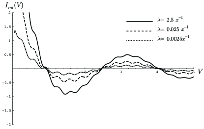
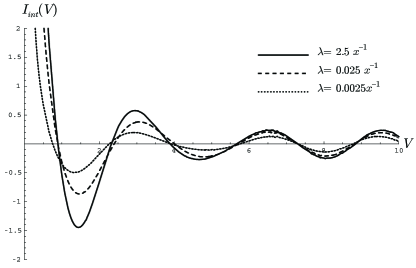
Figure 2: The interference term in the current as a function of applied voltage at low temperature, for $v_{n}=0.1\,v_{c}$ (upper panel) and $v_{n}=0.75\,v_{c}$ (lower panel). The three curves in each are three different bulk-edge coupling strengths $\lambda={h^{2}}/2{v_{n}^{2}}$, given in units of $1/{x_{a}}$, the inverse of the separation between the point contacts.

However, for larger voltages $V\approx 10-100\mu$V and/or larger interferometers $2{x_{a}}\approx 10\mu\mbox{m}$, which are also experimentally accessible (see Ref. Zhang09, ), oscillations with voltage will be observed for even quasiparticle number, as shown, for instance, in Fig. 3 of Ref. Bishara08, . There are ‘fast’ oscillations with period in $V$ given roughly by $\frac{16\pi}{e|x_{1}-x_{2}|}(1/v_{n}+1/v_{c})^{-1}$ and ‘slow’ ones with larger period, $\frac{16\pi}{e|x_{1}-x_{2}|}(1/v_{n}-1/v_{c})^{-1}$. For an odd number of quasiparticles in the interferometer, one of which is close to an edge, oscillations are seen, but they are small for $\lambda\ll 1/{x_{a}}$. For $\lambda\gg x_{a}$, on the other hand, the interference term in the current approaches the even quasiparticle number case, as shown in Fig. 2. However, if ${e^{*}}V$ is not much smaller than ${v_{n}}/{x_{a}}$, this will occur in a more complicated way than in Eq. 28. For example, the nodes in the oscillations move as $\lambda$ is varied. Thus, if the voltage is near a nodal point in $I_{\rm int}(V)$, the current will not approach its $\lambda\rightarrow\infty$ value monotonically, as shown in Fig. 3.

Since the preceding formulas were computed perturbatively in the inter-edge backscattering operators, they are only valid for voltages which are not too small, i.e. so long as $|\Gamma_{a,b}|^{2}|{e^{*}}V|^{-1/2}\ll 1$. Thus, the crossover described above will be observable if there is a regime $|\Gamma_{a,b}|^{4}\ll{e^{*}}V\ll\frac{h^{2}}{v_{n}}$ (here, we have substituted $\lambda={h^{2}}/{2v_{n}^{2}}$). However, it is possible to go to voltages lower than $|\Gamma_{a,b}|^{4}$, while still remaining in the weak-backscattering regime, if the temperature is finite, since ${k_{B}}T$ will then cut off the flow of $\Gamma_{a,b}$.

Finite-temperature correlation functions can be obtained from zero-temperature ones such as (25) by a conformal map from the half-plane to the half-cylinder. This amounts to the following substitution.

$$\delta+i(t\pm x/v)\rightarrow\left({\sin\left(\pi T(\delta+i(t\pm x/v))\right)}\right){\pi T}$$ (29)

Since the charged and neutral mode velocities are different, we apply such a substitution separately to the charged and neutral sectors of the theory, which we can do only because they are decoupled in the weak-backscattering limit. The $I-V$ curves shown in Fig. 2 are computed at small but non-zero temperature. (Since the temperature acts as an infrared regulator, it calculationally convenient.)

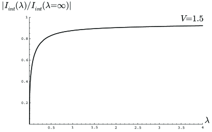
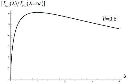
Figure 3: The amplitude of the interference term for fixed applied voltage ${e^{*}}V>{v_{n}}/2{x_{a}}$ as a function of bulk-edge coupling $\lambda$. $\lambda$ and ${e^{*}}V$ are measured in units of ${v_{n}}/2{x_{a}}$. The upper panel is away from a nodal point; the amplitude asymptotes its large $\lambda$ value at $\lambda\approx{v_{n}}/2{x_{a}}$. This represents the behavior of the envelope of the interference term; it agrees with the numerical calculation of Ref. Rosenow07b, . The lower panel is for $V$ near a nodal point in $I_{\rm int}$; the amplitude varies non-monotonically with $\lambda$ because the nodes move as $\lambda$ is varied.

VI Discussion

Until very recently, the evidence that the $\nu=5/2$ state is in the universality class of either the Moore-Read Pfaffian state Moore91 or the anti-Pfaffian state LeeSS07 ; Levin07 was derived entirely from numerical solutions of small systems Morf98 ; Rezayi00 . However, recent point-contact tunneling Radu08 and shot-noise Dolev08 experiments are consistent with these non-Abelian states. Even more recently, measurements Willett09 with a two point-contact interferometer appear consistent with the odd-even effect Bonderson06a ; Stern06 . In this paper, we have computed how the coupling of a bulk $e/4$ quasiparticle to the edge leads to a crossover between the odd and even quasiparticle number regimes. Our results may be relevant to the transition regime between different quasiparticle numbers in the experiment of Ref. Willett09, . We have made specific predictions in Eqs. 28 for how the interference term scales with voltage and temperature when there is appreciable bulk-edge coupling. If the transition regions can be studied as a function of temperature and voltage, a comparison may be possible.

Following Willett et al. Willett09 , let’s assume that $\Delta\Phi=c\Delta V_{s}$ for some constant $c$, where $V_{s}$ is the sidegate voltage. When a bulk quasiparticle is close to the edge, $h$ will be large, the dependence of $h$ on $V_{g}$ will be complicated. However, for some range of $V_{s}$, $h$ will be approximately $h\sim e^{-r/\xi}$, where $r$ is the distance to the edge and $\xi$ is a length scale corresponding to the size of the Majorana bound state at the bulk $e/4$ quasiparticle. If $r={r_{0}}-b{V_{s}}$, then one might expect $h={h_{0}}e^{b{V_{s}}}$ for some $h_{0}$, $b$. We take Willett et al.’s $c$ and choose ${h_{0}},b$ so that the quasiparticle is effectively absorbed by the edge after $\sim 5$ periods. To compare with the results of Ref. Willett09, , we must add to (28) the contribution of charge $e/2$ quasiparticles:

$$I^{\left(e/2\right)}=\frac{e}{2}\,\frac{2\pi}{v_{c}}\Bigl{(}|\Gamma_{a}^{e/2}|^{2}+\left|\Gamma_{b}^{e/2}\right|^{2}\Bigr{)}\\ +2\cdot\frac{e}{2}\,\frac{2\pi}{v_{c}}\,\,\text{Re}\left\{\Gamma_{a}^{e/2}(\Gamma_{b}^{e/2})^{*}e^{2\pi i(\frac{\Phi}{2\Phi_{0}}-\frac{{n_{q}}}{4})}\right\}$$ (30)

Figure 4: The backscattered current $I_{B}$ (normalized by its maximum value) as a function of sidegate voltage $V_{s}$ (in mV), assuming that there is an odd number of $e/4$ quasiparticles in the interference loop, one of which is close to the edge. The bulk-edge coupling is assumed to vary with sidegate voltage as $h={h_{0}}e^{b{V_{s}}}$ while the flux through the loop varies as $\Delta\Phi=c\Delta V_{s}$. A contribution to the current from charge $e/2$ quasiparticles (with period $2\Phi_{0}$) is also included with an amplitude which is approximately half the large-$h$ limit of the amplitude of the period $4\Phi_{0}$ oscillations.

If we assume that the backscattered $e/2$ quasiparticle contribution to the current is half as large as the (large-$\lambda$ limit of the) $e/4$ contribution (although this is a somewhat questionable assumption in general, it may hold over a range of temperatures, see e.g. Ref. Bishara09, ), then we can obtain the total backscattered current as a function of $V_{s}$, as shown in Fig. 4. A striking feature of this plot is that, for large $h$, the $e/2$ oscillation (with period $2\Phi_{0}$) is masked by the larger $e/4$ oscillation (with period $4\Phi_{0}$). We emphasize that the amplitude of the $e/2$ oscillation is not changing with $V_{s}$, as may be seen from Eq. 30; the apparent suppression of the $e/2$ oscillation as the amplitude of the $e/4$ oscillation increases is illusory. This is reminiscent of a salient feature of Willett et al.’s Willett09 data: in the regions in which $e/4$ oscillations are visible, $e/2$ oscillations are often barely, if at all, visible. The apparent disappearance of the $e/2$ oscillation in Fig. 4 results, in part, from the $\pi/4$ phase shift of the $e/4$ oscillation in Eq. 28, which helps it submerge the smaller $e/2$ oscillation. This suggests that some of the regions in Willett et al.’s Willett09 data which have been interpreted as having an even number of quasiparticles in the interference loop because of the presence of $e/4$ oscillations may, in fact, have an odd number of quasiparticles in the loop, one of which is close enough to the edge that $\lambda$ is large and the quasiparticle is effective absorbed, as in Fig. 4 for ${V_{s}}>70\,\text{mV}$. If this is true, then we would expect that, if ${v_{n}}\lambda$ is much smaller than the energy gap $\Delta$ of the $\nu=5/2$ quantum Hall state, then as the temperature is raised above ${v_{n}}\lambda$, the $e/4$ oscillation will disappear (due to both the effective decoupling of one of the quasiparticles from the edge and also thermal smearing of the $e/4$ oscillation Wan08 ; Bishara09 ) and only the $e/2$ oscillation will be left. Finally, it is amusing to note that if we assume that $h$ increases even more sharply with ${V_{s}}$, e.g. $h={h_{0}}e^{b{V_{s}^{2}}}$, then the $e/2$ oscillation seemingly disappears even more suddenly.

In this paper, we have focussed on the case of an odd number of quasiparticles in the bulk, one of which is coupled to the edge. The case of an even number of quasiparticles is qualitatively different: in the absence of bulk-edge coupling, interference is observed, with a phase which is determined by the combined topological state of the quasiparticles in the bulk. For instance, when there are two quasiparticles in an interference loop, they form a qubit (or half a qubit, if four quasiparticles with total topological charge $1$ are used to represent a qubit) DasSarma05 ; Nayak08 . Bulk-edge coupling then leads to errors in this qubit and, over long enough time scales, to the disappearance of this qubit as one of the bulk quasiparticles is absorbed by the edge. This non-equilibrium problem will be the subject of a separate work.

Figure 5: If we assume that $h$ increases more sharply with $V_{s}$, e.g. $h={h_{0}}e^{bV_{s}^{2}}$, then the apparent disappearance of $e/2$ oscillations (with period $2\Phi_{0}$) as $h$ increases with $V_{s}$ is even more dramatic.

Appendix A Method of Chatterjee and Zamolodchikov

As a consequence of the mapping introduced in Section IV, we can reduce the problem of finding the interference term in the current backscattered in the interferometer to that of finding $\langle{\sigma_{1}}(z,\overline{z})\rangle_{\rm h}$ with $z,\overline{z}$ independent variables. Following Chatterjee and Zamolodchikov Chatterjee94 , we note that Eqs. 19 imply that

$$\left({\partial_{t}}+\frac{ih^{2}}{2v_{n}}\right)\!\psi_{1R}(0,t)=\left({\partial_{t}}-\frac{ih^{2}}{2v_{n}}\right)\!\psi_{1L}(0,t)$$ (31)

Thus, the combination on the right-hand-side of (31) is the continuation of the left-hand-side, simply reflected back by $x=0$, analogous to ${\psi_{R}}(0)={\psi_{L}}(0)$ for free boundary condition. Chatterjee and Zamolodchikov Chatterjee94 observe that this fact, which can be written in complex notation as

$$\left[({\partial_{z}}+i\lambda)\psi_{1R}-(\partial_{\overline{z}}-i\lambda)\psi_{1L}\right]_{z=\overline{z}}=0$$ (32)

where $\lambda={h^{2}}/2{v_{n}^{2}}$, allows them to treat $({\partial_{z}}+i\lambda)\psi_{1R}$ as a free field unaffected by the boundary interaction.

Now, consider the quantity $\langle\psi_{1R}(z){\mu_{1}}(w,\overline{w})\rangle$, where ${\mu_{1}}(w,\overline{w})$ is the disorder operator dual to ${\sigma_{1}}(w,\overline{w})$,

$${\psi_{R}}(z)\cdot{\sigma_{1}}(w,\overline{w})=\frac{\omega}{\sqrt{2}}\,{\mu_{1}}(w,\overline{w})+\ldots$$ (33)

For fixed boundary condition, $\langle\psi_{1R}(z){\mu_{1}}(w,\overline{w})\rangle$ can be deduced by scaling and the requirement of square root branch points at $w$ and $\overline{w}$:

$$\left\langle\psi_{1R}(z)\,{\mu_{1}}(w,\overline{w})\right\rangle_{\rm fixed}=\frac{(w-\overline{w})^{3/8}}{(z-w)^{1/2}(z-\overline{w})^{1/2}}$$ (34)

Thus, for fixed boundary condition,

$$\left\langle({\partial_{z}}+i\alpha)\psi_{1R}(z)\,{\mu_{1}}(w,\overline{w})\right\rangle_{\rm fixed}(z-w)^{1/2}(z-\overline{w})^{1/2}=\\ \frac{A(w,\overline{w})}{z-w}+\frac{\overline{A}(w,\overline{w})}{z-\overline{w}}+B(w,\overline{w})$$ (35)

holds for arbitrary $\alpha$ with

$$A(w,\overline{w})=\overline{A}(w,\overline{w})=iB(w,\overline{w})/2\alpha=-\frac{1}{2}(w-\overline{w})^{3/8}$$ (36)

For free boundary condition, $\langle\psi_{1R}(z){\mu_{1}}(w,\overline{w})\rangle$ vanishes by fermion number parity, so (35) holds trivially with $A(w,\overline{w})=\overline{A}(w,\overline{w})=B(w,\overline{w})=0$. For non-zero $h$, Eq. 35 must hold for the special value $\alpha=\lambda$ since $({\partial_{z}}+i\lambda)\psi_{1R}(z)$ is a free field, i.e. this correlation function’s only singularities are square root branch points at $w$ and $\overline{w}$:

$$\left\langle\,{\chi_{R}}(z){\mu_{1}}(w,\overline{w})\right\rangle_{h}(z-w)^{1/2}(z-\overline{w})^{1/2}=\\ \frac{A(w,\overline{w})}{z-w}+\frac{\overline{A}(w,\overline{w})}{z-\overline{w}}+B(w,\overline{w})$$ (37)

where

$${\chi_{R}}(z)\equiv({\partial_{z}}+i\lambda)\psi_{1R}(z)$$ (38)

but $A(w,\overline{w})$, $\overline{A}(w,\overline{w})$. However, $B(w,\overline{w})$ in (37) will no longer have their free field forms (36). In the $z\rightarrow w$ limit, (37) becomes

$$\left\langle\,{\chi_{R}}(z){\mu_{1}}(w,\overline{w})\right\rangle_{h}=(z-w)^{-3/2}\frac{A(w,\overline{w})}{(w-\overline{w})^{1/2}}\\ \ -\frac{1}{2}(z-w)^{-1/2}\frac{A(w,\overline{w})}{(w-\overline{w})^{3/2}}+\frac{3}{8}(z-w)^{1/2}\frac{A(w,\overline{w})}{(w-\overline{w})^{5/2}}\\ +(z-w)^{-1/2}\frac{\overline{A}(w,\overline{w})}{(w-\overline{w})^{3/2}}-\frac{3}{2}(z-w)^{1/2}\frac{\overline{A}(w,\overline{w})}{(w-\overline{w})^{5/2}}\\ +(z-w)^{-1/2}\frac{B(w,\overline{w})}{(w-\overline{w})^{1/2}}-\frac{1}{2}(z-w)^{1/2}\frac{B(w,\overline{w})}{(w-\overline{w})^{3/2}}$$ (39)

On the other hand, the operator product expansion of ${\chi_{R}}(z)\equiv({\partial_{z}}~{}+~{}i\lambda)\psi_{1R}(z)$ with ${\mu_{1}}(w,\overline{w})$ is determined by the short-distance properties of the theory, i.e. ${\mu_{1}}$ is still simply the operator which creates a branch cut for $\psi_{1R}$, even in the presence of a boundary magnetic field. Thus, this OPE can be computed using $S_{0}$:

$${\chi_{R}}(z)\,\cdot\,{\mu_{1}}(w,\overline{w})=\frac{\overline{\omega}}{\sqrt{2}}\Bigl{[}(z-w)^{-3/2}\left(-\mbox{$\frac{1}{2}$}{\sigma_{1}}(w,\overline{w})\right)\\ +(z-w)^{-1/2}(2{\partial_{w}}+i\lambda){\sigma_{1}}(w,\overline{w})\\ +(z-w)^{1/2}(4{\partial^{2}_{w}}+4i\lambda{\partial_{w}}){\sigma_{1}}(w,\overline{w})+\ldots\Bigr{]}$$ (40)

where $\omega=e^{i\pi/4}$.

Taking the ground state expectation values of both sides of (40) and comparing corresponding powers of $z-w$ with (39) leads to the equations:

$$\frac{A(w,\overline{w})}{(w-\overline{w})^{1/2}}=\frac{\overline{\omega}}{\sqrt{2}}\left[-\frac{1}{2}\left\langle{\sigma_{1}}(w,\overline{w})\right\rangle\right]$$ (41)

$$-\frac{1}{2}\frac{A(w,\overline{w})}{(w-\overline{w})^{3/2}}+\frac{\overline{A}(w,\overline{w})}{(w-\overline{w})^{3/2}}\>+\\ \frac{B(w,\overline{w})}{(w-\overline{w})^{1/2}}=\frac{\overline{\omega}}{\sqrt{2}}\left[(2{\partial_{w}}+i\lambda)\left\langle{\sigma_{1}}(w,\overline{w})\right\rangle\right]$$ (42)

$$\frac{3}{8}\frac{A(w,\overline{w})}{(w-\overline{w})^{5/2}}-\frac{3}{2}\frac{\overline{A}(w,\overline{w})}{(w-\overline{w})^{5/2}}\>-\\ \frac{1}{2}\frac{B(w,\overline{w})}{(w-\overline{w})^{3/2}}=\frac{\overline{\omega}}{\sqrt{2}}\left[(4{\partial^{2}_{w}}+4i\lambda{\partial_{w}})\left\langle{\sigma_{1}}(w,\overline{w})\right\rangle\right]$$ (43)

Substituting (41) into (42), leads to

$$B(w,\overline{w})+\frac{\overline{A}(w,\overline{w})}{(w-\overline{w})}=\\ \frac{\overline{\omega}}{\sqrt{2}}(w-\overline{w})^{1/2}\!\left(2{\partial_{w}}+i\lambda-\frac{1}{4}\frac{1}{w-\overline{w}}\right)\left\langle{\sigma_{1}}(w,\overline{w})\right\rangle$$ (44)

and substituting (44) into (43) leads to

$$-\frac{\overline{A}(w,\overline{w})}{(w-\overline{w})^{5/2}}=\frac{\overline{\omega}}{\sqrt{2}}(w-\overline{w})^{1/2}\biggl{[}4{\partial^{2}_{w}}+4i\lambda{\partial_{w}}+\frac{1}{w-\overline{w}}{\partial_{w}}\\ +\frac{1}{2}i\lambda\frac{1}{w-\overline{w}}-\frac{1}{16}\frac{1}{(w-\overline{w})^{2}}\biggr{]}\!\!\left\langle{\sigma_{1}}(w,\overline{w})\right\rangle$$ (45)

Proceeding in a precisely analogous manner, similar equations can be derived for the OPE and correlation function of ${\chi_{L}}(\overline{z})\equiv(\partial_{\overline{z}}~{}-~{}i\lambda)\psi_{1L}(\overline{z})$ and ${\mu_{1}}(w,\overline{w})$, from which it follows that:

$$\frac{\overline{A}(w,\overline{w})}{(\overline{w}-w)^{1/2}}=\frac{\omega}{\sqrt{2}}\left[-\frac{1}{2}\left\langle{\sigma_{1}}(w,\overline{w})\right\rangle\right]$$ (46)

$$B(w,\overline{w})+\frac{A(w,\overline{w})}{\overline{w}-w}=\\ \frac{\omega}{\sqrt{2}}(\overline{w}-w)^{1/2}\!\left(2\partial_{\overline{w}}-i\lambda-\frac{1}{4}\frac{1}{\overline{w}-w}\right)\left\langle{\sigma_{1}}(w,\overline{w})\right\rangle$$ (47)

$$-\frac{A(w,\overline{w})}{(\overline{w}-w)^{5/2}}=\frac{\omega}{\sqrt{2}}(w-\overline{w})^{1/2}\biggl{[}4{\partial^{2}_{\overline{w}}}-4i\lambda{\partial_{\overline{w}}}+\frac{1}{\overline{w}-w}{\partial_{\overline{w}}}\\ -\frac{1}{2}i\lambda\frac{1}{w-\overline{w}}-\frac{1}{16}\frac{1}{(w-\overline{w})^{2}}\biggr{]}\!\!\left\langle{\sigma_{1}}(w,\overline{w})\right\rangle$$ (48)

Eqs. 41 and 46 imply that $A(w,\overline{w})=-\overline{A}(w,\overline{w})$. This relation allows us to take the difference between Eqs. 44 and 47 to find

$$\left({\partial_{w}}+\partial_{\overline{w}}\right)\left\langle{\sigma_{1}}(w,\overline{w})\right\rangle=0$$ (49)

Chatterjee and Zamolodchikov Chatterjee94 specialize to the case $w=-\overline{w}=ix$, but this is not necessary. At no point in the preceding derivation, leading to Eqs. 44, 45, 47, 48, do we need $w=(\overline{w})^{*}$. Thus, we can take $w={v_{n}}{\tau_{0}}+i{x_{a}}$ and $\overline{w}={v_{n}}{\tau}-i{x_{a}}$. Then, $w+\overline{w}={v_{n}}(\tau+{\tau_{0}})$, so that Eq. 49 states that the correlation function is time-translation invariant, as expected. Hence, without loss of generality, we can set ${\tau_{0}}=0$ so that $w=i{x_{a}}$ and $\overline{w}={v_{n}}{\tau}-i{x_{a}}$.

Since the correlation function is independent of $w+\overline{w}$, we can rewrite (41) as an ordinary differential equation in terms of the scaling variable $y=-i\lambda(w-\overline{w})=\lambda(2{x_{a}}+i{v_{n}}\tau)$:

$$\left[-4{\partial_{y}^{2}}+\left(4-\mbox{$\frac{1}{y}$}\right){\partial_{y}}+\left(\mbox{$\frac{1}{2y}-\frac{9}{16}\frac{1}{y^{2}}$}\right)\right]\langle{\sigma_{1}}(y)\rangle=0$$ (50)

We warn the reader that there is a typo in Ref. Chatterjee94, , where $1/y$ appears instead of $1/2y$ in the third term.

If we let $\langle{\sigma_{1}}(y)\rangle\equiv y^{3/8}\,f(y)$, then

$$yf^{\prime\prime}+(1-y)f^{\prime}-\mbox{$\frac{1}{2}$}f=0$$ (51)

This is Kummer’s equation, $yf^{\prime\prime}+(b-y)f^{\prime}-af=0$, with $a=\frac{1}{2}$ and $b=1$. It has two linearly independent solutions. The confluent hypergeometric function (or Kummer’s function) of the first kind, denoted by ${{}_{1}F_{1}}(a,b,y)$ or $M(a,b,y)$, diverges exponentially for large $y$. The other solution is the confluent hypergeometric function (or Kummer’s function) of the second kind, denoted by $U(a,b,y)$. When $\text{Re}(y)>0$, it has the integral representation

$$U(a,b,y)=\frac{1}{\Gamma(a)}{\int_{0}^{\infty}}\!dt\,e^{-ty}\,t^{a-1}\,(1+t)^{b-a-1}$$ (52)

The confluent hypergeometric functions are singular at $y=0,\infty$ and can be elsewhere in terms of formal power series.

From the integral representation (52), we see that $U(a,b,y)$ decays as $1/y^{a}$ for large $y$. Hence, this is the appropriate solution for $\langle{\sigma_{1}}(y)\rangle$, leading to $\langle{\sigma_{1}}(y)\rangle=({\rm const.})\,\times\,y^{3/8}\,\,U(\frac{1}{2},1,y)$. The constant is fixed Chatterjee94 by matching to the lowest order perturbative calculation so that it agrees for small $y$ with, for example, Ref. Overbosch07, ; Rosenow07b, :

$$\langle{\sigma_{1}}(w,\overline{w})\rangle=\lambda^{1/2}\,2^{1/4}\,y^{3/8}\,\,U\!\left(\mbox{$\frac{1}{2}$},1,y\right)$$ (53)

where $y=-i\lambda(w-\overline{w})$.

Appendix B Continuous Neumann and Continuous Dirichlet Fixed Points

The crossover discussed in this paper can also be formulated in terms of an Ising model with a defect line, rather than a boundaryFendley09 . According to this alternative mapping, the top and bottom edges become the left- and right-moving sectors of the Ising model. The ‘defect line’ is the middle of the device, $x=0$, where we have put a bulk quasiparticle. There are quotation marks in the previous sentence because it may not be clear that there is actually a defect at $x=0$ until one considers the fact that the correlation function between the tunneling operators at the two point contacts $\langle{T_{a}}(0){T_{b}^{\dagger}}(\tau)\rangle$, translates to the correlation between two Ising spin operators, one to the left and one to the right of the defect, $\langle\sigma(x,0)\,\sigma(x^{\prime},\tau)\rangle$ with $xx^{\prime}<0$. (Note that we have formed non-chiral Ising spins in a different way than we did in Section IV; they are formed from chiral fields on opposite edges.) With a quasiparticle in the bulk (which we have not yet coupled to the edge), this correlation function vanishes. Thus, the defining feature of the defect line is that this correlation function vanishes but correlation functions of spin fields all of which are to the right of the defect line or all of which are to the left of the defect line are precisely the same as if there were no defect, as if there were no bulk quasiparticle.

This defect line doesn’t have a simple interpretation in the classical $2D$ Ising model, but it does in the $(1+1)$-D transverse field Ising model, where it corresponds to the quantum Hamiltonian Oshikawa97 :

$$H=-h{\sum_{n\neq 0}}{\sigma^{x}_{n}}-J{\sum_{n\neq 0}}{\sigma^{z}_{n-1}}{\sigma^{z}_{n}}-{J^{\prime}}\sigma^{z}_{-1}{\sigma^{x}_{0}}$$ (54)

with $h=J$ in order to tune to criticality and, for the moment, we specialize to $J^{\prime}=J$. At the critical point, we can take the continuum limit, with $x=na$, where $a$ is the lattice spacing. The Hamiltonian (54) has the aforementioned property, $\langle\sigma(x,\tau)\,\sigma(x^{\prime},\tau^{\prime})\rangle=0$ for $xx^{\prime}<0$, since it is obtained from the usual critical $(1+1)$-D transverse field Ising model by performing a duality transformation

$${\sigma_{n}^{z}}\rightarrow{\mu_{m}^{z}} = \prod_{0\leq m\leq n}{\sigma^{x}_{n}}$$ (55)

$${\sigma_{n}^{x}}\rightarrow{\mu_{n}^{x}} = {\sigma^{z}_{n}}\sigma^{z}_{n+1}$$ (56)

on only half of the chain, $n\geq 0$. Thus, the correlation function $\langle\sigma(x,\tau)\,\sigma(x^{\prime},\tau^{\prime})\rangle=0$ with $xx^{\prime}<0$ is equal to $\langle\mu(x,\tau)\,\sigma(x^{\prime},\tau^{\prime})\rangle=0$ in the ordinary critical $(1+1)$-D transverse field Ising model. The latter correlation function, between an order and a disorder field, vanishes.

In fact, this property holds all along the fixed line obtained by varying $J^{\prime}$, which was dubbed the continuous Neumann line in Ref. Oshikawa97, . As discussed in Ref. Fendley09, , varying $J^{\prime}$ corresponds to pinching the quantum Hall bar so that interedge backscattering of Majorana fermions (but not of charged quasiparticles) can occur at $x=0$. When Majorana fermions are also allowed to tunnel from the edges to the bulk $e/4$ quasiparticle at $x=0$, the system flows from the continuous Neumann line to the continuous Dirichlet line, at which the bulk $e/4$ quasiparticle at $x=0$ has been absorbed by the edge(s). The continuous Dirichlet line is described by the critical transverse field Ising model with one bond weakened/strengthened:

$$H=-h{\sum_{n\neq 0}}{\sigma^{x}_{n}}-J{\sum_{n\neq 0}}{\sigma^{z}_{n-1}}{\sigma^{z}_{n}}-\tilde{J}\sigma^{z}_{-1}{\sigma^{z}_{0}}$$ (57)

In this paper, we consider the special case in which there is no constriction at $x=0$, so that there is no interedge backscattering of Majorana fermions at $x=0$. Furthermore, the bulk $e/4$ quasiparticle at $x=0$ is close to only one edge. Thus, our flow is a special case of the continuous Neumann to continuous Dirichlet flow discussed in Refs. Oshikawa97, ; Fendley09, . The combination of Ising correlation functions which enters the formula (24) for the current is simply $\langle\sigma(x,\tau)\,\sigma(-x,\tau^{\prime})\rangle=0$. The nice feature of this formulation is that it refers only to explicitly single-valued correlation functions in a perturbed version of 54.

$$U(n+1/2,1,y)=e^{y/2}{K_{n}}(y/2)/\sqrt{\pi}$$

- (1) C. de C. Chamon et al., Phys. Rev. B 55, 2331 (1997).
- (2) E. Fradkin, C. Nayak, A. Tsvelik, and F. Wilczek, Nucl. Phys. B 516, 704 (1998).
- (3) F. E. Camino, W. Zhou, and V. J. Goldman, Phys. Rev. B 72, 075342 (2005).
- (4) R. Willett et al., Phys. Rev. Lett. 59, 1776 (1987).
- (5) J. P. Eisenstein, K. B. Cooper, L. N. Pfeiffer, and K. W. West, Phys. Rev. Lett. 88, 076801/1 (2002).
- (6) J. S. Xia et al., Phys. Rev. Lett. 93, 176809 (2004).
- (7) G. Moore and N. Read, Nucl. Phys. B 360, 362 (1991).
- (8) M. Greiter et al., Nucl. Phys. B 374, 567 (1992).
- (9) C. Nayak and F. Wilczek, Nucl. Phys. B 479, 529 (1996).
- (10) D. A. Ivanov, Phys. Rev. Lett. 86, 268 (2001).
- (11) P. Bonderson, A. Kitaev, and K. Shtengel, Phys. Rev. Lett. 96, 016803 (2006).
- (12) A. Stern and B. I. Halperin, Phys. Rev. Lett. 96, 016802 (2006).
- (13) B. J. Overbosch and X.-G. Wen, arXiv:0706.4339.
- (14) W. Bishara and C. Nayak, Phys. Rev. B 77, 165302 (2008).
- (15) R. L. Willett, L. N. Pfeiffer, and K. W. West, to appear in Proc. natl. Acad. Sci. USA (2009), arXiv:0807.0221.
- (16) W. Bishara, P. Bonderson, C. Nayak, K. Shtengel, and J. Slingerland, arXiv:0903.3108.
- (17) P. Fendley, M.P.A. Fisher, and C. Nayak, arXiv:0902.0998.
- (18) R. Chatterjee and A. Zamolodchikov, Mod. Phys. Lett. A 9, 2227 (1994). (arXiv:hep-th/9311165).
- (19) R. Chatterjee, Mod. Phys. Lett. A10, 973 (1995).
- (20) B. Rosenow, B. I. Halperin, S. Simon, and A. Stern, Phys. Rev. Lett. 100, 226803 (2008).
- (21) M. Milovanović and N. Read, Phys. Rev. B 53, 13559 (1996).
- (22) C. Bena and C. Nayak, Phys. Rev. B 73, 155335 (2006).
- (23) P. Fendley, M. P. A. Fisher, and C. Nayak, Phys. Rev. Lett. 97, 036801 (2006).
- (24) P. Fendley, M. P. A. Fisher, and C. Nayak, Phys. Rev. B 75, 045317 (2007).
- (25) X. Wan, K. Yang, and E. H. Rezayi, Phys. Rev. Lett. 97, 256804 (2006).
- (26) Y. Zhang, D. T. McClure, E. M. Levenson-Falk, C. M. Marcus, L. N. Pfeiffer, K. W. West, arXiv:0901.0127.
- (27) N. Read and E. Rezayi, Phys. Rev. B 54, 16864 (1996).
- (28) N. Read and D. Green, Phys. Rev. B 61, 10267 (2000).
- (29) E. Ardonne and E.-A. Kim, arXiv:0705.2902 (unpublished).
- (30) L. Fidkowski, arXiv:0704.3291 (unpublished).
- (31) J. Cardy, Nucl. Phys. B 324, 581 (1989).
- (32) S.-S. Lee, S. Ryu, C. Nayak, and M. P. Fisher, Phys. Rev. Lett. 99, 236807 (2007).
- (33) M. Levin, B. I. Halperin, and B. Rosenow, Phys. Rev. Lett. 99, 236806 (2007).
- (34) R. H. Morf, Phys. Rev. Lett. 80, 1505 (1998).
- (35) E. H. Rezayi and F. D. M. Haldane, Phys. Rev. Lett. 84, 4685 (2000).
- (36) I. Radu, J. Miller, C. Marcus, M. Kastner, L. N. Pfeiffer, K. West, Science 320, 899 (2008).
- (37) M. Dolev, M. Heiblum, V. Umansky, A. Stern, and D. Mahalu, Nature 452, 829 (2008).
- (38) S. Das Sarma, M. Freedman, and C. Nayak, Phys. Rev. Lett. 94, 166802 (2005).
- (39) C. Nayak et al., Rev. Mod. Phys. 80, 1083 (2008).
- (40) M. Oshikawa and I. Affleck, Nucl. Phys. B 495, 533 (1997). [arXiv:cond-mat/9612187]
- (41) X. Wan et al., Phys. Rev. B77, 165316 (2008).
- (42) B. Rosenow et al.,