Comparing neutron star predictions by various microscopic models

Abstract

We calculate several neutron star properties, for static and/or rotating stars, using equations of state based on different microscopic models. These include our Dirac-Brueckner-Hartree-Fock model and others derived from the non-relativistic Brueckner-Hartree-Fock approach implemented with microscopic three-body forces. The model dependence is discussed.

I Introduction

The determination of the equation of state (EoS) of highly compressed and/or hot matter is one of the most complex problems in nuclear physics. In terrestrial laboratories, relativistic heavy-ion collisions are the best tool to produce hot and dense matter. Concerning astrophysical systems, neutron stars are known to be stable configurations containing the most dense form of matter found in the universe. They are therefore unique laboratories to study the properties of highly compressed (cold) matter. Furthermore, the possibility of studying the structure of neutron stars via gravitational waves GW makes these exotic objects even more exciting.

More generally, the study of neutron-rich systems (from the lowest to the highest densities) has widespread impact, reaching from the physics of exotic nuclei to nuclear astrophysics. With the Facility for Rare Isotope Beams (FRIB) recently approved for design and construction at Michigan State University, these studies become particularly important and timely. Partnership between nuclear physics and astrophysics will play a crucial role in advancing our knowledge of neutron-rich matter and its equation of state.

Clearly, a rich (on-going or future) experimental program must be accompanied by parallel theoretical effort. Present nuclear matter calculations are typically performed either within the mean field approach or the microscopic one. Mean field models, relativistic and non-relativistic, are popular Sk ; RMF , but in our opinion ab initio approaches are best in order to get deeper physical insight. By ab initio, we mean that the starting point is a realistic two-body potential, possibly complemented by three-body forces.

The purpose of this paper is to compare several neutron star properties predicted by different microscopic models. As constraints promise to become more stringent, it is important to understand and compare how the nature of the various predictions is related to the features of each model. In microscopic approaches, the tight connection with the underlying two-body potential will then facilitate the physical understanding in terms of the characteristics of the nuclear force and its behavior in the medium.

In the next section, we review the main aspects of the ab initio approach. The main differences between our approach (the Dirac-Brueckner-Hartree-Fock method) and the other models used in our comparison (the conventional Brueckner-Hartree-Fock method together with microscopic three-body forces) are revisited and discussed.

II The “ab initio” approach

II.1 The two-body framework

Our present knowledge of the nuclear force is the result of decades of struggle Mac89 . After the development of QCD and the understanding of its symmetries, chiral effective theories chi became popular as a way to respect the symmetries of QCD while keeping the degrees of freedom (nucleons and pions) typical of low-energy nuclear physics. However, chiral perturbation theory (ChPT) has definite limitations as far as the range of allowed momenta is concerned. For the purpose of applications in dense matter, where higher and higher momenta become involved with increasing Fermi momentum, ChPT is inappropriate. A relativistic, meson-theoretic model is the better choice.

The one-boson-exchange (OBE) model has proven very successful in describing nucleon-nucleon (NN) data in free space and has a good theoretical foundation. Among the many available OBE potentials (some being part of the “high-precision generation” pot1 ; pot2 ; pot3 ), we seek a momentum-space potential developed within a relativistic scattering equation, such as the one obtained through the Thompson three-dimensional reduction of the Bethe-Salpeter equation. Furthermore, we require a potential that uses the pseudovector coupling for the interaction of nucleons with pseudoscalar mesons. With this in mind, as well as the requirement of a good description of NN data, Bonn B Mac89 has been our standard choice. As is well known, the NN potential model dependence of nuclear matter predictions is not negligible. The saturation points obtained with different NN potentials move along the famous “Coester band” depending on the strength of the tensor force, with the weakest tensor force corresponding to the largest attraction. For the same reason (that is, the role of the tensor force in nuclear matter), the potential model dependence is strongly reduced in pure (or nearly pure) neutron matter, due to the absence of isospin-zero partial waves.

Already when QCD (and its symmetries) were unknown, it was observed that the contribution from the nucleon-antinucleon pair diagram, Fig. 1, is unreasonably large when the pseudoscalar (ps) coupling is used, leading to very large pion-nucleon scattering lengths GB79 . We recall that the Lagrangian density for pseudoscalar coupling of the nucleon field ($\psi$) with the pseudoscalar meson field ($\phi$) is

$${\cal L}_{ps}=-ig_{ps}\bar{\psi}\gamma_{5}\psi\phi.$$ (1)

On the other hand, the same contribution (Fig. 1) is heavily suppressed by the pseudovector (pv) coupling (a mechanism which became known as “pair suppression”). The reason for the suppression is the presence of the covariant derivative at the pseudovector vertex,

$${\cal L}_{pv}=\frac{f_{ps}}{m_{ps}}{\bar{\psi}}\gamma_{5}\gamma^{\mu}\psi\partial_{\mu}\phi,$$ (2)

which suppresses the vertex for low momenta and, thus, explains the small value of the pion-nucleon scattering length at threshold GB79 . Considerations based on chiral symmetry GB79 can further motivate the choice of the pseudovector coupling. We will come back to this point in the next subsection.

The most important aspect of the “ab initio” approach is that the only free parameters of the model (namely, the parameters of the NN potential) are determined by the fit to the free-space data and never readjusted in the medium. In other words, the model parameters are tightly constrained and the calculation in the medium is parameter free. The presence of free parameters in the medium would generate effects and sensitivities which can be very large and hard to control.

Figure 1: Contribution to the NN interaction from virtual pair excitation. Upward- and downward-pointing arrows represent nucleons and antinucleons, respectively. Dashed lines denote mesons.

II.2 The many-body framework: Brueckner theory, three-body forces, and relativity

Excellent reviews of Brueckner theory have been written which we can refer the reader to (see Mac89 and references therein). Here, we begin by defining the contributions that are retained in our calculation. Those are the lowest order contribution to the Brueckner series (two-hole lines) and the corresponding exchange diagram. With the G-matrix as the effective interaction, this amounts to including particle-particle (that is, short-range) correlations, which are absolutely essential to even approach a realistic description of nuclear matter properties. Three-nucleon correlations have been shown to be small if the continuous choice is adopted for the single-particle potential Baldo98 .

The issue of three-body forces (TBF), of course, remains to be discussed. In Fig. 2 we show a TBF originating from virtual excitation of a nucleon-antinucleon pair, known as “Z-diagram”. Notice that the observations from the previous section ensure that the corresponding diagram at the two-body level, Fig. 1, is small with pv coupling. At this point, it is useful to recall the main feature of the Dirac-Brueckner-Hartree-Fock (DBHF) method, as that turns out to be closely related to the TBF depicted in Fig. 2. In the DBHF approach, one describes the positive energy solutions of the Dirac equation in the medium as

$$u^{*}(p,\lambda)=\left(\frac{E^{*}_{p}+m^{*}}{2m^{*}}\right)^{1/2}\left(\begin{array}[]{c}{\bf 1}\\ \frac{\sigma\cdot\vec{p}}{E^{*}_{p}+m^{*}}\end{array}\right)\;\chi_{\lambda},$$ (3)

where the effective mass is given by $m^{*}=m+U_{S}$, with $U_{S}$ an attractive scalar potential. It turns out that both the description of a single-nucleon via Eq. (3) and the evaluation of the Z-diagram, Fig. 2, generate a repulsive effect on the energy/particle in symmetric nuclear matter which depends on the density approximately as

$$\Delta E\propto\left(\frac{\rho}{\rho_{0}}\right)^{8/3},$$ (4)

and provides the saturating mechanism missing from conventional Brueckner calculations. Brown showed that the bulk of this effect can be obtained as a lowest order (in $p^{2}/m$) relativistic correction to the single-particle propagation GB87 .

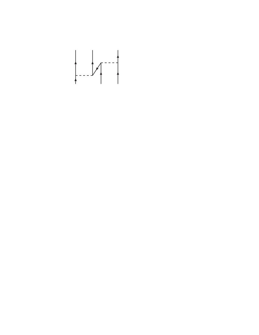
Figure 2: Three-body force due to virtual pair excitation. Conventions as in the previous figure.

The approximate equivalence of the effective-mass spinor description and the contribution from the Z-diagram has a simple intuitive explanation in the observation that Eq. (3), like any other solution of the Dirac equation, can be written as a combination of positive and negative energy solutions. On the other hand, the “nucleon” in the middle of the Z-diagram, Fig. 2, is precisely a superposition of positive and negative energy states. In summary, the DBHF method effectively takes into account a particular class of TBF, which are crucial for nuclear matter saturation, but does not include other TBF.

Concerning other, more popular, three-body forces, Fig. 3 shows the TBF that is included in essentially all TBF models, regardless other components; it is the Fujita-Miyazawa TBF FM . With the addition of contributions from $\pi N$ S-waves, one ends up with the well-known Tucson-Melbourne TBF TM . The microscopic TBF of Ref. Catania include contributions from excitations of the Roper resonance (P₁₁ isobar) as well.

Now, if diagrams such as the one shown on the left-hand side of Fig. 3 are included, consistency requires that medium modifications at the corresponding two-body level are also included, that is, the diagram on the right-hand side of Fig. 3 should be present and properly medium modified. Large cancellations then take place, a fact that was brought up a long time ago DMF . When the two-body sector is handled via OBE diagrams, the two-pion exchange is effectively incorporated through the $\sigma$ “meson”, which cannot generate the (large) medium effects (dispersion and Pauli blocking on $\Delta$ intermediate states) required by the consistency arguments above.

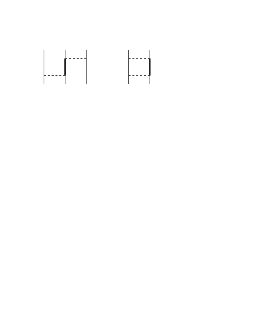
Figure 3: Left: three-body force arising from $\Delta$-isobar excitation (thick line). Right: two-meson exchange contribution to the NN interaction involving $\Delta$-isobar excitation.

To contrast this point of view, we will take as the other elements of our comparison the EoS’s from the microscopic approach of Ref. cat . There (and in previous work by the authors Catania ), the Brueckner-Hartree-Fock (BHF) formalism is employed along with microscopic three-body forces. However, in Ref. Catania the meson-exchange TBF are constructed applying the same parameters as used in the corresponding nucleon-nucleon (NN) potentials, which are: Argonne V18 (V18, V18 ), Bonn B (BOB, Mac89 ), Nijmegen 93 (N93, pot2 ). The popular (but phenomenological) Urbana TBF (UIX, UIX ) is also utilized in Ref. cat along with the V18 potential. The parameters which are not specified by the NN potential are chosen according to independent investigations Catania . Convenient parametrizations in terms of simple analytic functions are given in all cases for the resulting EoS’s. We will refer to this approach, generally, as “BHF + TBF”.

In a previous work SL09 we compared the predictions of the neutron skin in ²⁰⁸Pb by these models and correlated them with differences in the slope of the symmetry energy. Model differences become larger at high-density and will naturally impact neutron star predictions.

III Neutron stars: Results and discussion

Stellar matter contains neutrons in $\beta$ equilibrium with protons, electrons, and muons. Our DBHF EoS for $\beta$-equilibrated matter is given in Ref. Sam0806 . We have applied $\beta$-stability in the same way to the various models of Ref. cat starting from the given parametrized versions of the respective symmetric matter and neutron matter EoS’s. At subnuclear densities, all the EoS’s considered here are joined with the crustal equations of state from the work of Harrison and Wheeler HW (for energy densities between 10 and 10¹¹ g cm^-3) and the work of Negele and Vautherin NV (for energy densities less than 1.7$\times$10¹³g cm^-3). The composition of the crust is crystalline, with light HW or heavy NV metals and electron gas. The DBHF equation of state as applied in this work, including the crust, is given in the tables. All neutron star properties are calculated using public software downloaded from the website http://www.gravity.phys.uwm.edu/rns.

In Fig. 4, we show the mass-radius relation for a sequence of static neutron stars as predicted by the various models listed above. All models besides DBHF share the same many-body approach but differ in the two-body potential and TBF employed. The resulting differences can be much larger than those originating from the use of different many-body approaches. This can be seen by comparing the DBHF and BOB curves, both employing the Bonn B interaction. Overall, the maximum masses range from 1.8$M_{\odot}$ (UIX) to 2.5$M_{\odot}$ (BOB). Radii are less sensitive to the EoS and range between 10 and 12 km for all models under consideration, DBHF or BHF+TBF. Concerning available constraints, an initial observation of a neutron-star-white dwarf binary system suggested a neutron star mass (PSR J0751+1807) of 2.1$\pm$0.2$M_{\odot}$ Nice . Such observation would imply a considerable constraint on the high-density behavior of the EoS. On the other hand, a dramatically reduced value of 1.3$\pm$0.2$M_{\odot}$ was recently reported Piek08 , which does not invalidate any of the theoretical models under consideration.

The model dependence is shown in Fig. 5 for the case of rapidly rotating stars. The 716 Hz frequency corresponds to the most rapidly rotating pulsar, PSR J1748-2446 Hessels , although recently an X-ray burst oscillation at a frequency of 1122 Hz has been reported Kaaret which may be due to the spin rate of a neutron star. As expected, the maximum mass and the (equatorial) radius become larger with increasing rotational frequency.

Another bulk property of neutron stars is the moment of inertia, $I$. In Fig. 6, we show the moment of inertia at different rotational speeds (again, for all models), whereas in Fig. 7 we display the moment of inertia corresponding to the maximum mass at different rotational frequencies. These values are not in contraddiction with observations of the Crab nebula luminosity. From that, a lower bound on the moment of inertia was inferred to be $I\geq$4-8 $\times$ 10⁴⁴ g cm², see Ref. Weber and references therein. The size of $I_{M_{max}}$ changes from model to model in line with the size of the maximum mass, see Fig. 7. (We recall that the variations among radii from different EoS’s are relatively mild).

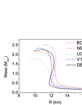
Figure 4: (color online) Static neutron star mass-radius relation for the models considered in the text.

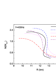
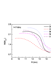
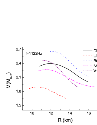
Figure 5: (color online) Mass-radius relation for the models considered in the text and for different rotational frequencies.

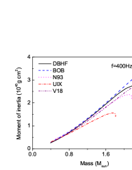
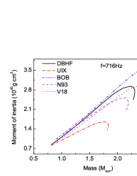
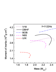
Figure 6: (color online) Moment of inertia for the models considered in the text and for different rotational frequencies.

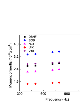
Figure 7: (color online) Moment of inertia corresponding to the maximum mass for the models considered in the text as a function of the rotational frequency.

Lastly, we calculate the gravitational redshift predicted by each model. The redshift is defined as

$$z=\Big{(}1-\frac{2M}{R}\Big{)}^{-1/2}-1\;.$$ (5)

This simple formula can be derived considering a photon emitted at the surface of a neutron star and moving towards a detector located at large distance. The photon frequency at the emitter (receiver) is the inverse of the proper time between two wave crests in the frame of the emitter (receiver). Assuming a static gravitational field, and writing $g_{00}$ as the metric tensor component at the surface of a nonrotating star yield the equation above. Naturally the rotation of the star modifies the metric, and in that case different considerations need to be applied which result in a frequency dependence of the redshift. We will not be calculating the general case here.

From Fig. 8, it appears that the gravitational redshift is not very EoS-dependent (compare, for instance, the values at the maximum mass for each model), an indication that the gravitational profile at the surface of the star is similar in all models. Thus measurements of $z$ may not be the best way to discriminate among EoS’s.

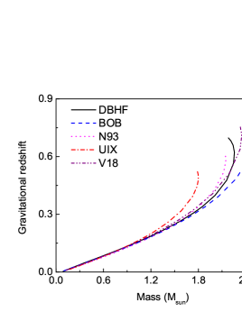
Figure 8: (color online) Gravitational redshift for all models. For each model, the corresponding sequence of static stars is considered.

IV Summary and conclusions

We stress the importance of ab initio calculations to complement the wealth of present/future experiments and observations aimed at constraining the less known aspects of the nuclear equation of state. In that spirit, we have undertaken a comparison of EoS-sensitive observables in microscopic models, which do or do not include explicit TBF. In a previous work SL09 we related different predictions of the neutron skin in ²⁰⁸Pb to differences in the slope of the symmetry energy. An accurate measurement of the neutron skin, as expected to be taken at the Jefferson Laboratory Jlab , is the most promising way to discriminate among EoS’s in the low-density regime.

At the high-densities probed by neutron stars, the model dependence is even larger, however, presently available constraints are still insufficient to discriminate among these EoS’s.

At high density ($\rho$ between five and ten times normal density), the most repulsive symmetric matter energies are produced with BOB, V18, DBHF, N93 and UIX, in that order. That is consistent with the maximum mass predictions, which depend mostly on the absolute repulsion present in the symmetric matter EoS. In pure neutron matter, N93 follows right after BOB (again, from largest to smallest repulsion). This indicates a somewhat different balance when only T=1 contributions are included. Finally, the symmetry energy, which depends entirely on the repulsion of neutron matter relative to symmetric matter and whose density dependence controls observables such as the neutron skin, is largest in N93, followed by BOB, V18, UIX, and DBHF.

The model dependence we observe comes from two sources, the two-body potential and the many-body approach, specifically the presence of explicit TBF or Dirac effects. The dependence on the two-body potential is very large. Typically, the main source of model dependence among NN potentials is found in the strength of the tensor force. Of course, differences at the two-body level impact the TBF as well, whether they are microscopic or phenomenological (as in the case of UIX).

On the other hand, when comparing DBHF and BOB, we are looking at differences stemming from the many-body scheme, as the two models share the same NN potential. In the BOB model, repulsion grows at a much faster rate than in DBHF, and more strongly so in neutron matter. (Hence, the much larger symmetry energy with BOB SL09 ). As an example, at about 6 times normal density the DBHF energy of symmetric matter is 67% of the BOB energy and only 51% at ten times normal densities. In pure neutron matter, those ratios become 49% and 30%, respectively. Thus, the inclusion of the microscopic TBF in the BHF model introduces considerable more repulsion than the Dirac effects (whose density dependence is approximately as given in Eq. (4)), through highly non-linear terms cat . Both attractive and repulsive TBF are required for a realistic description of the saturation point. The density dependence of the repulsive terms is obviously stronger and thus dominate at high density. Furthermore, it appears that this is especially true in neutron matter. The much larger (compared with DBHF) repulsion in neutron matter (relative to symmetric matter) seen in all BHF+TBF models may be due to the attractive nature of some T=0 NN partial waves, most noticeably ${}^{3}S_{1}$, which, on the other hand, would become repulsive at high density in the presence of Dirac effects. This attractive component (not present in neutron matter) can moderate the repulsion arising from TBF.

At this time, available constraints cannot pin down the high-density behavior of the EoS. Nevertheless, our point is that microscopic models allow for a deeper insight into the origin of the observed physical effects, and should be pursued along with improved constraints.

Table 1: Equation of state for $\beta$-equilibrated matter. At subnuclear densities the crustal EoS from Refs. HW ; NV is given. At normal to super-high densities the DBHF equation of state is shown.

Baryon density(1/$cm^{3}$)	Energy density($g/cm^{3}$)	Pressure($dyne/cm^{2}$)
0.59701000E+25	0.99998600E+01	0.40721410E+12
0.75334200E+25	0.12618390E+02	0.15080560E+13
0.11995300E+26	0.20092030E+02	0.10132810E+14
0.19099900E+26	0.31992190E+02	0.47174340E+14
0.24101400E+26	0.40369630E+02	0.94073580E+14
0.30412500E+26	0.50940640E+02	0.18050450E+15
0.38376300E+26	0.64279760E+02	0.33550870E+15
0.48425400E+26	0.81112010E+02	0.60721550E+15
0.61105800E+26	0.10235170E+03	0.10743490E+16
0.15492600E+27	0.25949850E+03	0.88776630E+16
0.19549400E+27	0.32745010E+03	0.14569410E+17
0.24668500E+27	0.41319610E+03	0.23670880E+17
0.31128200E+27	0.52139300E+03	0.38114990E+17
0.39279300E+27	0.65792350E+03	0.60884010E+17
0.49564800E+27	0.83020530E+03	0.96560320E+17
0.62543700E+27	0.10476010E+04	0.15215920E+18
0.12566500E+28	0.21048780E+04	0.57628220E+18
0.20009400E+28	0.33515470E+04	0.13693280E+19
0.25249000E+28	0.42291870E+04	0.20992040E+19
0.31860600E+28	0.53366300E+04	0.32077510E+19
0.40203500E+28	0.67340590E+04	0.48872650E+19
0.50731100E+28	0.84974150E+04	0.74261220E+19
0.64015400E+28	0.10722520E+05	0.11256160E+20
0.12862200E+29	0.21544010E+05	0.38701870E+20
0.20480200E+29	0.34304300E+05	0.87378890E+20
0.25843000E+29	0.43286960E+05	0.13099750E+21
0.32610100E+29	0.54622010E+05	0.19612730E+21
0.41149300E+29	0.68925200E+05	0.29327530E+21
0.51924500E+29	0.86973760E+05	0.43804640E+21
0.65521200E+29	0.10974830E+06	0.65359850E+21
0.13164600E+30	0.22050990E+06	0.21592540E+22
0.16611800E+30	0.27825210E+06	0.32107790E+22
0.20961700E+30	0.35111490E+06	0.47710750E+22
0.26450500E+30	0.44305570E+06	0.70850350E+22
0.33376600E+30	0.55907310E+06	0.10515070E+23
0.42116300E+30	0.70547070E+06	0.15597180E+23
0.53144400E+30	0.89020260E+06	0.23123900E+23
0.67060100E+30	0.11233090E+07	0.33677760E+23
0.17001500E+31	0.28479990E+07	0.13810890E+24
0.21453100E+31	0.35937570E+07	0.19523170E+24
0.27070400E+31	0.45348070E+07	0.27521560E+24
0.34158300E+31	0.57222920E+07	0.38687930E+24
0.43102100E+31	0.72207080E+07	0.54232090E+24
0.54387400E+31	0.91114890E+07	0.75808450E+24
0.68627500E+31	0.11497400E+08	0.10567510E+25
0.13787700E+32	0.23100980E+08	0.28166750E+25
0.21952400E+32	0.36783270E+08	0.53468330E+25
0.27699700E+32	0.46415170E+08	0.73411590E+25
0.34951600E+32	0.58569360E+08	0.10057550E+26
0.44101900E+32	0.73906140E+08	0.13750910E+26
0.55647700E+32	0.93259070E+08	0.18764540E+26
0.70215700E+32	0.11767960E+09	0.25560490E+26
0.17797700E+33	0.29836060E+09	0.86649420E+26
0.22456600E+33	0.37648930E+09	0.11718980E+27
0.28334500E+33	0.47507410E+09	0.15831900E+27
0.35751000E+33	0.59947540E+09	0.21366950E+27
0.45108900E+33	0.75645300E+09	0.28810670E+27
0.56915000E+33	0.95453350E+09	0.38815460E+27
0.71811000E+33	0.12044860E+10	0.52255320E+27
0.14423300E+34	0.24200880E+10	0.12701340E+28
0.22959600E+34	0.38534730E+10	0.22901680E+28
0.28966900E+34	0.48625310E+10	0.30733120E+28
0.36545800E+34	0.61358160E+10	0.41227540E+28
0.46107400E+34	0.77425110E+10	0.55287600E+28
0.58169000E+34	0.97699500E+10	0.74121190E+28

TABLE I, cont.

Baryon density(1/$cm^{3}$)	Energy density($g/cm^{3}$)	Pressure($dyne/cm^{2}$)
0.73385500E+34	0.12328280E+11	0.99344590E+28
0.14734400E+35	0.24770450E+11	0.23888140E+29
0.18587600E+35	0.31256660E+11	0.31991950E+29
0.23448300E+35	0.39441580E+11	0.42838370E+29
0.29580200E+35	0.49769610E+11	0.57354730E+29
0.37313900E+35	0.62801930E+11	0.76780650E+29
0.47069400E+35	0.79247170E+11	0.10277560E+30
0.59374600E+35	0.99998600E+11	0.13755860E+30
0.10899500E+36	0.18374080E+12	0.15080040E+30
0.20791800E+36	0.35086530E+12	0.41327350E+30
0.30685800E+36	0.51813430E+12	0.66738040E+30
0.40581200E+36	0.68549240E+12	0.89490400E+30
0.50477400E+36	0.85290930E+12	0.10966500E+31
0.60373600E+36	0.10203670E+13	0.12773240E+31
0.80166500E+36	0.13553720E+13	0.15941520E+31
0.90062000E+36	0.15229090E+13	0.17377690E+31
0.10985200E+37	0.18580330E+13	0.20087290E+31
0.11974500E+37	0.20256030E+13	0.21397550E+31
0.13953200E+37	0.23608150E+13	0.23994040E+31
0.15931600E+37	0.26960450E+13	0.26615840E+31
0.16920800E+37	0.28636860E+13	0.27951740E+31
0.17910000E+37	0.30313280E+13	0.29309910E+31
0.19888300E+37	0.33666280E+13	0.32106350E+31
0.20877300E+37	0.35342880E+13	0.33549110E+31
0.21866300E+37	0.37019650E+13	0.35024070E+31
0.23844100E+37	0.40373370E+13	0.38075420E+31
0.24833000E+37	0.42050320E+13	0.39653560E+31
0.25821800E+37	0.43727450E+13	0.41267750E+31
0.26810600E+37	0.45404400E+13	0.42918160E+31
0.27799300E+37	0.47081710E+13	0.44605250E+31
0.28788000E+37	0.48758840E+13	0.46329190E+31
0.29776600E+37	0.50436140E+13	0.48089980E+31
0.30765200E+37	0.52113630E+13	0.49887950E+31
0.31753700E+37	0.53790930E+13	0.51722760E+31
0.32742200E+37	0.55468420E+13	0.53594420E+31
0.33730600E+37	0.57146080E+13	0.55502940E+31
0.34718900E+37	0.58823750E+13	0.57447980E+31
0.35707300E+37	0.60501410E+13	0.59429390E+31
0.36695600E+37	0.62179070E+13	0.61447010E+31
0.37683800E+37	0.63856910E+13	0.63500680E+31
0.38672000E+37	0.65534760E+13	0.65589600E+31
0.39660200E+37	0.67212770E+13	0.67714090E+31
0.40648400E+37	0.68890790E+13	0.69873660E+31
0.41636500E+37	0.70568810E+13	0.72068480E+31
0.42624500E+37	0.72246830E+13	0.74297430E+31
0.43612600E+37	0.73925030E+13	0.76560670E+31
0.44600500E+37	0.75603230E+13	0.78857870E+31
0.46576400E+37	0.78959800E+13	0.83552890E+31
0.47564200E+37	0.80638360E+13	0.85949750E+31
0.48552100E+37	0.82316740E+13	0.88379610E+31
0.49539800E+37	0.83995290E+13	0.90841830E+31
0.50527400E+37	0.85673840E+13	0.93336260E+31
0.51515000E+37	0.87352400E+13	0.95862580E+31
0.52502600E+37	0.89031130E+13	0.98420450E+31
0.53490100E+37	0.90709860E+13	0.10100920E+32
0.54477600E+37	0.92388600E+13	0.10362880E+32
0.55465100E+37	0.94067330E+13	0.10627910E+32
0.56452500E+37	0.95746240E+13	0.10896010E+32
0.57439900E+37	0.97425150E+13	0.11167080E+32
0.58427200E+37	0.99104240E+13	0.11441110E+32
0.59414500E+37	0.10078320E+14	0.11718180E+32
0.60401800E+37	0.10246220E+14	0.11998160E+32
0.61389000E+37	0.10414150E+14	0.12280980E+32
0.63363400E+37	0.10749990E+14	0.12855310E+32
0.65337700E+37	0.11085860E+14	0.13440860E+32

TABLE I, cont.

Baryon density(1/$cm^{3}$)	Energy density($g/cm^{3}$)	Pressure($dyne/cm^{2}$)
0.66324800E+37	0.11253780E+14	0.13737910E+32
0.67311800E+37	0.11421730E+14	0.14037590E+32
0.69285800E+37	0.11757640E+14	0.14645200E+32
0.70272800E+37	0.11925600E+14	0.14953050E+32
0.72246600E+37	0.12261520E+14	0.15576620E+32
0.73233400E+37	0.12429500E+14	0.15892440E+32
0.75207000E+37	0.12765460E+14	0.16531580E+32
0.76193800E+37	0.12933460E+14	0.16855220E+32
0.77180500E+37	0.13101440E+14	0.17181270E+32
0.79153800E+37	0.13437440E+14	0.17840720E+32
0.80140400E+37	0.13605450E+14	0.18174290E+32
0.82113400E+37	0.13941490E+14	0.18848650E+32
0.83099900E+37	0.14109500E+14	0.19189430E+32
0.85072800E+37	0.14445550E+14	0.19878210E+32
0.86059200E+37	0.14613590E+14	0.20226200E+32
0.87045500E+37	0.14781620E+14	0.20576440E+32
0.88031800E+37	0.14949670E+14	0.20929080E+32
0.89018100E+37	0.15117700E+14	0.21284120E+32
0.90990300E+37	0.15453810E+14	0.22001090E+32
0.91976300E+37	0.15621880E+14	0.22362710E+32
0.93948300E+37	0.15958020E+14	0.23093300E+32
0.94934200E+37	0.16126090E+14	0.23461640E+32
0.98877600E+37	0.16798420E+14	0.24958070E+32
0.14590200E+38	0.24523600E+14	0.41632200E+32
0.23168800E+38	0.38982700E+14	0.82280400E+32
0.34584300E+38	0.58250100E+14	0.14210400E+33
0.49242100E+38	0.83026900E+14	0.23006100E+33
0.67547500E+38	0.11401900E+15	0.40981400E+33
0.78194600E+38	0.13207300E+15	0.54012600E+33
0.89905700E+38	0.15195500E+15	0.71172400E+33
0.10273100E+39	0.17376500E+15	0.97049800E+33
0.11672200E+39	0.19760500E+15	0.13704600E+34
0.13192900E+39	0.22358900E+15	0.20162700E+34
0.14840200E+39	0.25183700E+15	0.26192800E+34
0.16619200E+39	0.28248100E+15	0.33029700E+34
0.18535000E+39	0.31568300E+15	0.51720500E+34
0.20592700E+39	0.35161900E+15	0.75702800E+34
0.22797300E+39	0.39049500E+15	0.11003700E+35
0.25153800E+39	0.43255500E+15	0.16084300E+35
0.27667400E+39	0.47813800E+15	0.23509200E+35
0.30343200E+39	0.52760100E+15	0.33455700E+35
0.33186100E+39	0.58135500E+15	0.46583400E+35
0.36201200E+39	0.63986100E+15	0.63214300E+35
0.39393700E+39	0.70359400E+15	0.83222800E+35
0.42768500E+39	0.77303000E+15	0.10713900E+36
0.46330800E+39	0.84870300E+15	0.13477500E+36
0.50085600E+39	0.93108800E+15	0.16560600E+36
0.54038000E+39	0.10206900E+16	0.20027100E+36
0.58193000E+39	0.11181400E+16	0.24141700E+36
0.62555700E+39	0.12243400E+16	0.29312500E+36
0.67131200E+39	0.13404700E+16	0.35869100E+36
0.71924500E+39	0.14679700E+16	0.44217300E+36
0.76940800E+39	0.16084100E+16	0.53909800E+36
0.82185000E+39	0.17629800E+16	0.64928300E+36
0.87662200E+39	0.19333700E+16	0.77966700E+36
0.93377600E+39	0.21214100E+16	0.93298700E+36
0.99336100E+39	0.23293000E+16	0.11139500E+37
0.10554300E+40	0.25594100E+16	0.13245200E+37
0.11200300E+40	0.28143700E+16	0.15691600E+37
0.11872100E+40	0.30972100E+16	0.18569700E+37
0.12570300E+40	0.34114400E+16	0.21904600E+37
0.13295400E+40	0.37606000E+16	0.25722700E+37
0.14047800E+40	0.41488100E+16	0.30137700E+37
0.14828000E+40	0.45806700E+16	0.35220200E+37
0.15636600E+40	0.50613000E+16	0.41065500E+37
0.16474100E+40	0.55963600E+16	0.47754300E+37
0.17341000E+40	0.61920200E+16	0.55414900E+37
0.18237800E+40	0.68552200E+16	0.64123300E+37

V Acknowledgments

Support from the U.S. Department of Energy under Grant No. DE-FG02-03ER41270 is acknowledged. We are grateful to F. Weber for providing the crustal EoS.

References

- (1) Benjamin J. Owen, arXiv:0903.2603 [astro-ph.SR].
- (2) Lie-Wen Chen, C.M. Ko, and Bao-An Li, Phys. Rev. C 72, 064309 (2005).
- (3) Lie-Wen Chen, C.M. Ko, and Bao-An Li, arXiv:0709.0900 [nucl-th], and references therein.
- (4) R. Machleidt, Adv. Nucl. Phys. 19, 189 (1989).
- (5) S. Weinberg, Physica 96A, 327 (1979); Phys. Lett. B251, 288 (1990).
- (6) R. Machleidt, Phys. Rev. C 63, 024001 (2001).
- (7) V.G.J. Stocks, R.A.M. Klomp, C.P.F. Terheggen, and J.J. de Swart, Phys. Rev. C 49, 2950 (1994).
- (8) R.B. Wiringa et al., Phys. Rev. C 51, 38 (1995).
- (9) G.E. Brown, in “Mesons in Nuclei”, M. Rho and D.H. Wilkinson eds., Vol. I, p.330, North-Holland, Amsterdam (1979).
- (10) H.Q. Song et al., Phy. Rev. Lett. 81, 1584 (1998).
- (11) G.E. Brown et al., Comments Nucl. Part. Phys. 17, 39 (1987).
- (12) J. Fujita and H. Miyazawa, Prog. Theor. Phys. 17, 360 (1957).
- (13) R.G. Ellis, S.A. Coon, and B.H.J. McKellar, Nucl. Phys. A438, 631 (1985).
- (14) W.H. Dickhoff, A. Faessler, and H. Müther, Nucl. Phys. A389, 492 (1982).
- (15) Z.H. Li et al., Phys. Rev. C 77, 034316 (2008).
- (16) Z.H. Li and H.-J. Schulze, Phys. Rev. C 78, 028801 (2008).
- (17) R.B. Wiringa, V.G.J. Stocks, and R. Schiavilla, Phys. Rev. C 51, 38 (1995).
- (18) S.C. Pieper, V.R. Pandharipande, R.B. Wiringa, and J. Carlson, Phys. Rev. C 64, 014001 (2001).
- (19) F. Sammarruca and P. Liu, Phys. Rev. C 79, 057301 (2009).
- (20) F. Sammarruca and P. Liu, arXiv:0806.1936 [nucl-th].
- (21) B.K. Harrison and J.A. Wheeler in Gravitation Theory and Gravitational Collapse (B.K. Harrison, K.S. Thorne, M. Wakano, and J.A. Wheeler, eds.), pp. 1-177, University of Chicago Press, Chicago (1965).
- (22) J.W. Negele and D. Vautherin, Nucl. Phys. A178, 123 (1973).
- (23) D.J. Nice et al., Astrophys. J. 634, 1242 (2005).
- (24) D.J. Nice, talk presented at the Conference “40 Years of Pulsars”, McGill University, Montreal, Canada, August 12-17 2007.
- (25) J.W.T. Hessels et al., Science 311, 1901 (2006).
- (26) P. Kaaret et al., arXiv:0611716 [astro-ph].
- (27) F. Weber in “Pulsars as Astrophysical Laboratories for Nuclear and Particle Physics”, Institute of Physics Publishing, Bristol and Philadelphia, 1999.
- (28) R.B. Wiringa, V.G.J. Stocks, and R. Schiavilla, Phys. Rev. C 63, 025501 (2001).