The nature of intrinsic fluctuations in cosmic diffuse radiation

Abstract

The spatial and temporal noise properties of diffuse radiation is investigated in the context of the cosmic microwave background (CMB), although generic formulae that enable application to any other forms of incoherent light of a prescribed energy spectrum are also provided. It is shown that the variance of fluctuations in the density and flux consists of two parts. First is a term from the spontaneous emission coefficient which is the contribution from a random gas of classical particles representing the corpuscular (photon) nature of light. Second is a term from the stimulated emission coefficient which leads to a ‘wave noise’, or more precisely the noise arising from the superposition of many plane waves of arbitrary phase - the normal modes of the radiation. The origin of this second term has never been elucidated before. We discussed one application. In the spatially homogeneous post-inflationary epochs when the universe was reheated to GUT temperatures, the thermal CMB density fluctuations on the horizon scale is of order the WMAP measured value of 10^-5. Beyond (larger than) the horizon, the power spectrum of perturbations could moreover assume the observed form of $P(k)\sim k$ if thermal diffusion to equilibrium does not merely involve classical particles, but also non-localized wave components. The outcome of our study clearly demonstrates that such components do indeed exist.

1. Introduction: radiation noise and Poisson statistics

The fluctuation properties of diffuse radiation is a topic of increasing importance, especially with the advent of cosmological probes like COBE and WMAP, as they measure the density perturbations of the early universe that seeded the formation of structures (Bennett et al 2003, Hinshaw et al 2007, Spergel et al 2007). Yet, aside from the extrinsic physical processes that generated and grew these seeds, the cosmic microwave background (CMB), along with other forms of diffuse sky background, has its own intrinsic noise. It is helpful to acquire a better understanding of this noise, so that at the very least one has a firm handle of what to expect even in the limit of a perfect instrument and a smooth sky (the latter from the ‘extrinsic’ standpoint).

The motivation of our present paper is to take a close look at the intrinsic properties of radiation noise, with the black body radiation (BBR) as our prime focus, although generalization will be made to include other types of diffuse emissions. In the field of optics, this investigation was initiated and vigorously pursued by several authors during the decade of 1950 – 60 (Purcell 1956, Hanbury Brown and Twiss 1957, Mandel 1958), and in recent times the work was continued mostly by researchers of ultrafast optics (Trebino 1997). Our purpose here is to further develop and articulate the findings of these authors in the context of astrophysical observations and interpretations.

We begin by revisiting BBR itself, by considering lengthscales and timescales short enough that any effects due to the Hubble expansion can be neglected. The probability of having the integer $n$ as occupation number of some normal mode $j$ is governed by Bose-Einstein (BE) statistics, as

$$P_{n}=\left(1-e^{-\beta\hbar\omega_{j}}\right)e^{-n\beta\hbar\omega_{j}},$$ (1)

where $\beta=1/(k_{B}T)$. The mean occupation number and its variance are, as a result,

$$\bar{n}_{j}=\frac{1}{e^{\beta\hbar\omega_{j}}-1},~{}{\rm and}~{}(\delta n_{j})^{2}=\frac{e^{\beta\hbar\omega_{j}}}{e^{\beta\hbar\omega_{j}}-1}.$$ (2)

Similar parameters for the energy contribution from this mode are $\bar{\epsilon}_{j}=\bar{n}_{j}\hbar\omega_{j}$ and $(\delta\epsilon_{j})^{2}=(\delta n_{j})^{2}\hbar^{2}\omega_{j}^{2}$. Since modes within any black body cavity of volume $V$ are independent, the variance of the total energy $\epsilon$ in this volume is simply $(\delta\epsilon)^{2}=\sum_{j}(\delta\epsilon_{j})^{2}$.

Now, taking the continuum limit and applying the usual phase space density formula for the number of electromagnetic wave modes per interval $d\omega$ of angular frequency

$$\sum_{j}\rightarrow 2\times\frac{V}{(2\pi)^{3}}\int d^{3}{\bf k},~{}{\rm or}~{}\frac{dn_{{\rm mode}}}{d\omega}=2\times\frac{\omega^{2}V}{2\pi^{2}c^{3}},$$ (3)

where the factor of two represents the polarization degrees of freedom, one obtains

$$\bar{\epsilon}=\frac{8\pi V(k_{B}T)^{4}}{(hc)^{3}}\int_{0}^{\infty}\frac{x^{3}dx}{e^{x}-1}=\frac{8\pi^{5}V(k_{B}T)^{4}}{15(hc)^{3}},$$

and

$$(\delta\epsilon)^{2}=\frac{8\pi V(k_{B}T)^{5}}{(hc)^{3}}\int_{0}^{\infty}\frac{x^{4}e^{x}dx}{(e^{x}-1)^{2}}=\frac{32\pi^{5}k_{B}^{5}T^{5}V}{15h^{3}c^{3}}.$$ (4)

Hence the contrast in $\epsilon$, or the energy density $u$, is

$$\left(\frac{\delta\epsilon}{\epsilon}\right)^{2}=\left(\frac{\delta u}{u}\right)^{2}=\frac{15h^{3}c^{3}}{2\pi^{5}Vk_{B}^{3}T^{3}}=\frac{16k_{B}}{3S},$$ (5)

in agreement with the derivation of Peebles 1993 ($S=4\bar{\epsilon}/(3T)$ is the entropy of the radiation).

An important point of physics has to be made about eq. (2). The variance $(\delta n_{j})^{2}$ in $n_{j}$ is greater than the mean $\bar{n}_{j}$, i.e. BBR noise does not precisely follow Poisson statistics. Yet the common misconception that in the complete (quantum) theory radiation noise arises solely from photon counting may still be defended. Thus, when integrated over all frequencies, eqs. (4) and (5) give the distinctly Poissonian behavior of $(\delta\epsilon/\epsilon)^{2}\sim 1/N$ where $N=\int d\bar{n}$ is the total number of photons in the cavity of volume $V$. Also, for the high frequency modes $x=\hbar\omega/(k_{B}T)\gg 1$, $(\delta n)^{2}\approx\bar{n}$, i.e. the discrete nature of radiation as randomly moving photons prevails there. However, by writing the variance as two terms,

$$(\delta n)^{2}=\bar{n}(\bar{n}+1),~{}{\rm or}~{}(\delta n)^{2}=\frac{e^{x}}{(e^{x}-1)^{2}}=\frac{1}{e^{x}-1}+\frac{1}{(e^{x}-1)^{2}}.$$ (6)

we see that the Poisson noise term $\bar{n}$ dominates at $x\gg 1$, whereas the $\bar{n}^{2}$ (rightmost) term is significant only at low frequencies $x\ll$ 1. Focussing upon the latter, we may apply the $x\ll$1 limit to eq. (4) and obtain, for a frequency interval $\delta x$ in this regime, $(\delta\epsilon)^{2}\sim x^{2}\delta x/h^{3}\sim\nu^{2}\delta\nu/(k_{B}T)^{3}$, so that the variance is no longer dependent upon $h$. Clearly here, we are dealing with noise of a ‘classical’ nature. But what exactly is it? The question has never been answered rigorously.

2. The precise origin of the non-Poisson component and its importance

One could take the questions raised above as a red herring, or at best pedagogical: what prevents one from simply appealing to radiation as an ensemble of photons, which in turn are bosons with the manifestly non-Poisson distribution of eq. (1)? In other words, one already has an exact theory of BE statistics that renders any ‘analysis’ like the previous paragraph quite obsolete. The answer is three-fold. Firstly, the application of BE statistics to systems of various sizes is non-trivial even for BBR. Results like eqs. (4) and (5) actually describe an incoherent ensemble of $\sim V/(\Delta\lambda)^{3}$ ‘pure BE’ systems with $\Delta\lambda$ denoting the bandwidth of the spectrum (i.e. the range of wavelengths within which most of the emitted flux resides); each of such systems corresponds to an elementary cell in the standard phase space quantization scheme. If e.g. the volume of space in question is $\lesssim\lambda^{3}$, coherence effects will play a role, modifying the variance from the form eqs. (4) or (5), see Mandel 1958 (also Purcell 1956; Hanbury Brown, and Twiss 1957). The same ‘partitioning’ phenomenon applies as well to intensity fluctuations $\delta I$ over time intervals large or small compared with $1/\Delta\omega$. Such behavior deserves further investigation, which is one purpose of this paper.

Secondly, from the standpoint of modeling cosmological structures there is especially a need to press for better understanding of the two terms in eq. (6). The primordial density perturbations that seeded structure formation have hitherto been characterized by the two-point correlation function $\xi(\mathbb{r}_{1}-\mathbb{r}_{2})$, the Fourier transform of which is the power spectrum $P(k)$, which describes how particles are positioned in space via a locally random (Poisson) process. If, however, during the radiation era the fluctuations have a component that cannot be described in terms of the distribution of classical Poisson particles at all, then the properties of $\xi(\mathbb{r}_{1}-\mathbb{r}_{2})$ must be inferred without this perspective, i.e. an altogether different microscopic treatment will be necessary instead.

Thirdly, in astrophysics and experimental optics one could easily envisage other types of radiation, such as the diffuse X-ray background, or simply any arriving signals of incoherent light - often known as white light. If the mean energy spectrum (more precisely spectral energy density) $\bar{\cal U}(\omega)$ of the radiation is known, can we infer the fluctuations in the energy density at any length scale, or the intensity measured over any time scale? Obviously, a clear picture of the origin of all the noises is prerequisite to the solution.

To elaborate upon this third point, let the mean occupation number per mode be $\bar{n}(\omega)$, so the mean energy density of all modes is

$$\bar{\cal U}=\frac{1}{\pi^{2}c^{3}}\int_{0}^{\infty}\omega^{2}\hbar\omega\bar{n}(\omega)d\omega=\int_{0}^{\infty}\bar{\cal U}(\omega)d\omega,$$ (7)

where, from eq. (3),

$$\bar{\cal U}(\omega)=\frac{\omega^{3}}{\pi^{2}c^{3}}\bar{n}(\omega).$$ (8)

Now the distribution $n(\omega)$ assumes, for a given value $\bar{n}(\omega)$, the most likely occurring form when its Entropy is maximized subject to this constraint on the mean, irrespective of whether each mode is in ‘internal equilibrium’ or not (if it is, the ‘most likely’ qualifier will be unnecessary, see Jaynes 1957 for the complete theory). Under the scenario of states being occupied with complete a priori freedom, i.e. boson systems with no prior restriction on $n$, the resulting $n(\omega)$ would have the variance of $[\delta n(\omega)]^{2}=\bar{n}(\omega)[\bar{n}(\omega)+1]$. Hence, as in eq. (7),

$$(\delta{\cal U})^{2}=\frac{1}{\pi^{2}c^{3}V}\int_{0}^{\infty}\omega^{2}(\hbar\omega)^{2}{\bar{n}(\omega)[\bar{n}(\omega)+1)]}d\omega=\frac{1}{V}\int_{0}^{\infty}\left[\hbar\omega{\cal U}(\omega)+\frac{\pi^{2}c^{3}{\cal U}^{2}(\omega)}{\omega^{2}}\right]d\omega.$$ (9)

If the radiation is BBR, i.e.

$${\cal U}(\omega)=U(\omega)=\frac{\hbar\omega^{3}}{\pi^{2}c^{3}}\frac{1}{e^{\beta\hbar\omega}-1},$$ (10)

it will be trivial to show that eq. (9) is then the same as eq. (4), with the Poisson and non-Poisson (or ‘wave’) noise given by the ${\cal U}(\omega)$ integral and the ${\cal U}^{2}(\omega)$ integral respectively.

In spite of the elegance of the above derivation, one still ought to seek a more substantive physical justification of eq. (9) that does not appeal to any line of reasoning based upon the ‘game of chances’ of Jaynes 1957. We only resorted to such an argument because of our lack of fundamental understanding of the non-Poisson noise.

3. A heuristic treatment of wave superposition noise

The ‘$n^{2}$-noise’ contribution to the total variance of BBR fluctuations may further be elucidated, even if still heuristically, by Maxwell’s wave model of the radiation. Let BBR modes exist in the usual manner within some volume $V$. The normalized electric field of mode $j$ is written as

$${\bf E}_{j}({\bf r},t)=E_{j}{\bf e}_{j}\exp i({\bf k}_{j}\cdot{\bf r}-\omega_{j}t);{\bf E}_{j}({\bf r},t=0)=E_{j}{\bf e}_{j}\exp(i{\bf k}_{j}\cdot{\bf r}),$$ (11)

where ${\bf e}_{j}$ is the polarization unit vector. The total energy is $\epsilon=uV=V\sum_{j}|E_{j}|^{2}$. It seems reasonable to assume that $E_{j}$ are uncorrelated random variables, with a gaussian distribution of zero mean and variance $\langle|E_{j}|^{2}\rangle\sim\langle\epsilon_{j}\rangle/V$, where $\langle\epsilon_{j}\rangle$ is as defined in the text following eq. (2). Thus, the variance $(\delta\epsilon)^{2}$ is the sum of the individual $(\delta\epsilon_{j})^{2}$, i.e.

$$(\delta\epsilon)^{2}=V^{2}\sum_{j}[\langle|E_{j}|^{4}\rangle-(\langle|E_{j}|^{2}\rangle)^{2}].$$ (12)

For a complex gaussian random variable of zero mean, the second last term is twice the last term, so that

$$(\delta\epsilon)^{2}=\sum_{j}\langle\epsilon_{j}\rangle^{2}=\frac{8\pi V(kT)^{5}}{(hc)^{3}}\int_{0}^{\infty}\frac{x^{4}dx}{(e^{x}-1)^{2}},$$ (13)

which is the integrated contribution to the total variance from the ‘non Poisson’ (rightmost) term of eq. (6).

It should be clarified that classically the random complex nature of the field amplitude $E_{j}$ is due to the wave phase $\phi_{j}$ (which changes from mode to mode without correlation) rather than the photon counting noise, which is why the variance is not associated with Poisson statistics. In fact, we can rewrite eq. (7) as

$${\bf E}_{j}({\bf r},t)=|E_{j}|{\bf e}_{j}\exp i({\bf k}_{j}\cdot{\bf r}-\omega_{j}t+\phi_{j}),$$ (14)

where $|E_{j}|^{2}=U(\omega_{j})$ and $U$ is as defined in eq. (10). In the next section we proceed to perform a more rigorous calculation of this wave noise (or, better still, phase noise), by first attempting just the one dimensional problem of intensity fluctuations at various time scales.

4. Intensity fluctuation due to random mode phases, the coherence length of BBR

The total intensity (or flux, in ergs cm^-2 s^-1) of, for simplicity, a collimated beam of BBR arriving at the observer’s point ${\bf r}=0$ is given by

$$I(\tau)=\frac{1}{\tau}\int_{-\tau/2}^{\tau/2}~{}c|{\bf E}(t)|^{2}dt,$$ (15)

where $\tau$ is the time interval over which the intensity is measured, and

$${\bf E}(t)=\sum_{j}{\bf E}_{j}(t),$$ (16)

with ${\bf E}_{j}(t)={\bf E}_{j}({\bf r}=0,t)$ and the right side is as defined in eq. (14).

We shall soon see that $I(\tau)$ is a sum of two terms. One is a constant ‘DC’ term, independent of $\tau$ in particular, while the other is a random ‘AC’ term of zero mean, the variance of which decreases with increasing $\tau$. This second term causes $I(\tau)$ as evaluated by means of eq. (15) with different ‘time origins’ to fluctuate from one interval of duration $\tau$ to the next. The behavior is actually well known in optics (Trebino et al 1997), and is a consequence of the Uncertainty Principle. To see this readily, one could return to eq. (14) and set

$$\phi_{j}=0~{}~{}{\rm for~{}all}~{}j.$$ (17)

The sum over $j$ performed in eq. (16) to obtain the total wave electric field would then be, in essence, a Fourier inverse transform of the Planck function (more precisely $\sqrt{U(\omega)}$). The result is a ‘pulse’ of duration $\Delta t\sim 1/\Delta\omega$, where $\Delta\omega$ is the spectral width of $U(\omega)$, as is apparent when one plots the intensity profile $I(\tau)$ against $\tau$ with high time resolution, Figure 1. This scenario is known in the field of Fourier optics as a ‘transform limited pulse’, viz. the Uncertainty Principle is satisfied in the ‘minimal wave packet’ sense of $\Delta\omega\Delta t\sim 1$, and it is attained by setting all the mode phases to the same value - the highest degree of spectral phase coherence that can only be found in laser light.

If, as is normally the case of ordinary ‘white light’, the normal modes have more complicated phase relationships than eq. (17), the corresponding pulse will in general last longer than the minimum duration, i.e. it will satisfy $\Delta\omega\Delta t>1$. When the other end of the extreme is reached, such that the phases $\phi_{j}$ exhibit the maximum complexity by assuming uncorrelated random numbers as their values, one is dealing with ‘ideal white light’ (BBR falls under this category), viz. an arbitrarily long and continuous pulse with $\Delta\omega\Delta t\gg 1$ (Trebino et al 1997). Nevertheless, this continuous light train is in detail broken into many ‘spikes’ of all widths, ranging from one period of electric field oscillation at the BBR peak frequency to the full span of $L/c$. Such ‘spikes’ are to be realized in the ‘AC’ term of the previous paragraph.

To substantiate these points, we numerically computed eqs. (14) through (16) at two different resolutions $\tau$, one beneath the reciprocal bandwidth of the 3K BBR spectrum (i.e. $\tau\ll 1/\Delta\omega$) and the other well above it, this time assigning random phases $\phi_{j}$ to each mode $j$ as is appropriate for the BBR. The light intensity averaged over temporally contiguous intervals of $\tau$, $I(\tau)$, is indeed now seen in Figure 1c and Figure 2 to be continuous, yet it is equally obvious that there are hardly any changes in $I$ on the scale of $\tau\lesssim$ 10^-13 s; when $\tau$ is larger, at e.g. $\tau=$ 10^-10 s, noises then become apparent. In fact, as will be proved below, variations occur on all scales inside the range

$$\frac{1}{\Delta\omega}\lesssim\tau\lesssim\frac{1}{\delta\omega}$$ (18)

and with properties determined solely by the BBR spectrum $B(\omega)$ and independent of the mode quantization frequency $\delta\omega$ used in our simulation. For values of $\tau$ approaching the left inequality, the light curve becomes relaxed and regular, eventually altogether steady when $\tau\lesssim 1/\Delta\omega$ as Figure 2a reveals. This is consistent (again) with the Uncertainty Principle, viz. on timescales $\Delta t<1/\Delta\omega$ there can be no randomness in the signal. Far from this limit, the intensity turns erratic as the noise decorrelates from one resolution element $\tau$ to the next, Figure 2b. It should also be mentioned that the right inequality of eq. (18), viz. $\delta\omega\lesssim 1/\tau$, is equivalent to the constraint imposed by the periodic boundary condition as applied to a cube of side $L=c\tau$.

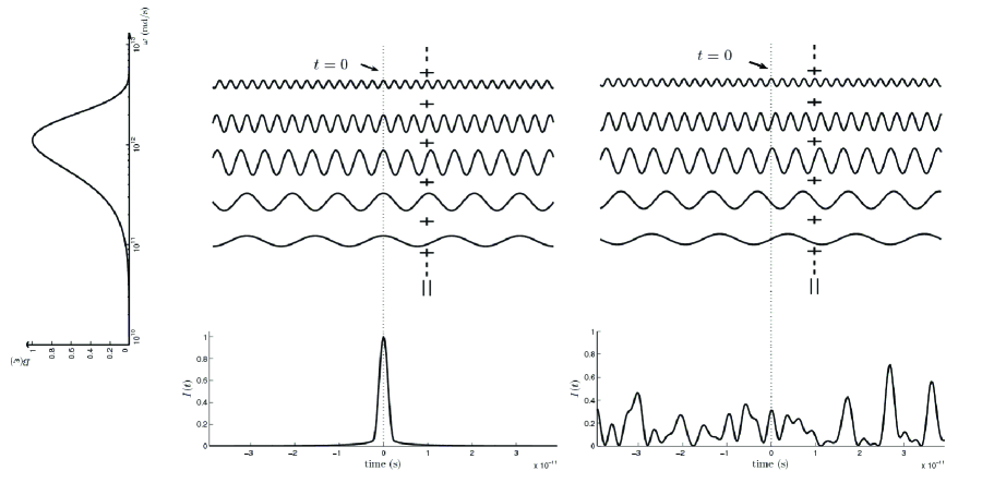
Figure 1: Two simulated intensity profiles (arbitrary units and photon Poisson noise excluded) of unpolarized light with the 3K black body spectrum of 1a (extreme left). The detector is assumed to be $\lesssim$ 1 cm, or one radiation wavelength, in width and length, to avoid complications due to spatial incoherence. Constituent normal modes are spaced $\delta\omega=$ 10¹⁰ rad/s apart. 1b (middle): all the modes are in phase, resulting in a single pulse which is the Fourier transform of the spectrum. The spectral width $\Delta\omega$ of 1a and the pulse width $\Delta t$ of 1b satisfy $\Delta\omega\Delta t\sim 1$. This is the scenario of a ‘transform limited pulse’ (or ‘minimal wave packet’), and occurs only when the modes have full phase correlation. 1c (right): the modes are randomly phased without any correlation among them; here we see an enduring light curve with aperiodic spikes and structures on all scales. Both profiles were constructed using eqs. (14) through (16), with a timing resolution of $\tau=$ 10^-14 s.

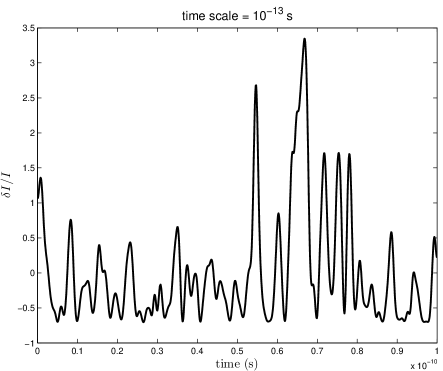
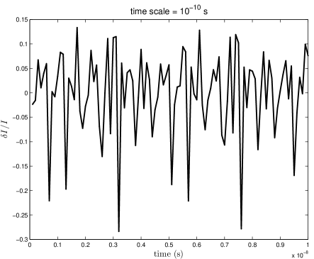
Figure 2: Intensity fluctuations (phase noise component) of 3K BBR as seen in two resolutions, 10^-13 s and 10^-10 s. Mode frequency spacing adopted by our simulation is $\delta\omega=$ 10¹⁰ rad/s as in Figure 1.

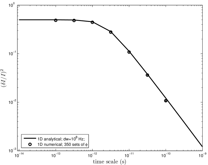
Figure 3: Power spectrum of temporal intensity fluctuations of 3K BBR, excluding photon Poisson noise. The uncertainties in the numerical simulations are $\lesssim$ the size of the circles, and are determined by generating data from 350 different sets of random phases $\phi_{j}$, then evaluating the scatter among the variances that result from each. The mode quantization adopted throughout is $\delta\omega=$ 10¹⁰ rad/s.

Our simulations for Figures 1 and 2 were pursued with a mode quantization $\delta\omega=$ 10¹⁰ rad/s. Further beyond plotting the intensity at the two $\tau$ values discussed, we calculated from such plots the normalized variance $(\delta I/I)^{2}$ (where $I$ is the ‘global’ mean intensity which is a constant independent of $\tau$) at each scale between $\tau=$ 10^-14 s and $\tau=$ 10^-10 s. The results are shown in Figure 3 as the data points of a power spectrum (in the WMAP sense of the words, i.e. fluctuation power at various scales). Towards $\tau=$ 10^-10 s the variance $\sim 1/\tau$, suggesting (as already said) that neighboring bins of $\tau$ decorrelate when $\tau$ becomes large. The argument is as follows. From eq. (15) the average intensity over some long interval ${\cal T}=N\tau$ may be written as

$$I_{{\cal T}}=c\times\frac{1}{{\cal T}}\left[\int_{0}^{\tau}|{\bf E}(t)|^{2}dt+\int_{\tau}^{2\tau}|{\bf E}(t)|^{2}dt+\cdots+\int_{(N-1)\tau}^{N\tau}|{\bf E}(t)|^{2}dt\right].$$ (19)

If each of the N terms on the right side fluctuates freely with a variance $\sigma_{\tau}^{2}$, we will have $(\delta I_{{\cal T}})^{2}=N\sigma_{\tau}^{2}/{\cal T}^{2}=\sigma_{\tau}^{2}/(N\tau^{2})$; but since $(\delta I_{\tau})^{2}=\sigma_{\tau}^{2}/\tau^{2}$ we obtain $(\delta I_{{\cal T}})^{2}=(\delta I_{\tau})^{2}/N$, or ${\cal T}(\delta I_{{\cal T}})^{2}=\tau(\delta I_{\tau})^{2}=$ constant. Hence $(\delta I_{{\cal T}})^{2}\sim 1/{\cal T}$. This trend holds as long as we compare two timescales in which the noise in the larger bin is simply the incoherent reinforcement of those in the smaller ones.

At $\tau\lesssim$ 10^-11 s, however, we see in Figure 3 a transition towards different behavior. As Figures 1c and 2a showed, the intensity changes over short intervals are regular and highly correlated, and variances no longer add. Eventually, $(\delta I_{{\cal T}})^{2}=(\delta I_{\tau})^{2}$ and the power spectrum flattens at the maximum, i.e. no ‘extra’ fluctuations may be found by measuring the intensity using more and more accurate clocks, so $\delta I$ does not rise any further. From Figure 3, one finds that the cross over point from constant $\delta I_{\tau}$ to the $\delta I_{\tau}\sim 1/\sqrt{\tau}$ dependence is at $\tau=\tau_{c}\approx$ 10^-10 s. This length may be used to define the coherence scale of BBR at $T=$ 3 K. Beneath $\tau_{c}$ (or $c\tau_{c}=$ 3 cm) a wavetrain of BBR exhibits good phase correlation, above it the phase becomes randomized. In another manner of expression, 3K radiation is capable of maintaining the integrity of its electromagnetic oscillation pattern for $\omega_{{\rm max}}\tau_{c}\approx$ 100 cycles. The overall picture is that one could divide space-time into many cells of this critical dimension, and assume coherence within each cell. Thus e.g. the point raised earlier in footnote 2 may now be understood in better terms: the power spectrum simulated and derived in this section is valid only for a detector size of $\lesssim$ 3 cm because we have not taken into account the additional effects of spatial incoherence.

Finally, it is also clear that the salient features of this section applies to diffuse radiation of any spectrum $B(\omega)$.

5. Analytical proof of temporal phase noise variance

The outcome of section 4 is not only relevant to BBR, but to incoherent light (or ‘white light’) with any broadband spectrum. A more rigorous mathematical proof to support the simulations is clearly desirable.

The intensity $I(\tau)$ at resolution $\tau$, eq. (15), has a ‘DC’ and an ‘AC’ contribution as mentioned after eq. (16). These may now be written as

$$I_{{\rm DC}}=\sum_{j}B_{j};~{}~{}I_{{\rm AC}}(\tau)=\sum_{{\bf k},m}\sum_{(\mathbb{k}^{\prime},n)\neq(\mathbb{k},m)}\mathbb{e}_{\mathbb{k},m}\cdot\mathbb{e}_{\mathbb{k}^{\prime},n}\sqrt{B_{k}B_{k^{\prime}}}\frac{\sin\left[\frac{(\omega_{k}-\omega_{k^{\prime}})\tau}{2}\right]}{(\omega_{k}-\omega_{k^{\prime}})\tau}e^{i\phi_{\mathbb{k},\mathbb{k}^{\prime},m,n}},$$ (20)

where $\phi_{\mathbb{k},\mathbb{k}^{\prime},m,n}=\phi_{\mathbb{k},m}-\phi_{\mathbb{k}^{\prime},n}$ ($m,n=$ 1,2 are polarization labels), $B_{k}=cU_{k}=\hbar kc^{2}/(e^{\beta\hbar ck}-1)$. Evidently $I_{{\rm DC}}$ is just a constant. Pairing each term in the series of $I_{{\rm AC}}$ with its complex conjugate, the $e^{i\phi}$ factor in eq. (20) is then replaced by $2\cos\phi$, and the $\sum_{\mathbb{k}^{\prime}}$ procedure is to be done with the understanding that only one member of every $(\mathbb{k},\mathbb{k}^{\prime})$ and $(\mathbb{k}^{\prime},\mathbb{k})$ pair should appear in the sum. The mean of $I_{{\rm AC}}$ is evidently zero. The variance is, in the continuum representation where $B(\omega)=cU(\omega)$ with the latter given by eq. (10),

$$(\delta I_{\tau})^{2}=\frac{2}{\tau^{2}}\int_{0}^{\infty}d\omega B(\omega)\int_{0}^{\infty}d\omega^{\prime}B(\omega^{\prime})\frac{\sin^{2}\left[\frac{(\omega^{\prime}-\omega)\tau}{2}\right]}{(\omega^{\prime}-\omega)^{2}},$$ (21)

after applying a correction factor of 1/2 to free the $\sum_{\mathbb{k}^{\prime}}$ step from the awkward ‘permutation’ restriction above; also the relation $\langle\cos^{2}\phi\rangle=$ 1/2 was used for the random phase differences $\phi$, and the sum over random polarizations follows the standard formula

$$\sum_{m}\sum_{n}({\bf e}_{{\bf k},m}\cdot{\bf e}_{{\bf k^{\prime}},n})^{2}=1+\left(\frac{{\bf k}\cdot{\bf k^{\prime}}}{kk^{\prime}}\right)^{2}=2$$ (22)

($\mathbb{k}\cdot\mathbb{k}^{\prime}\approx kk^{\prime}$ because $\omega^{\prime}\approx\omega$ as we saw, and $\mathbb{k}\|\mathbb{k}^{\prime}$ for a collimated beam), this sum replaces the factor of four from the helicity enumeration in the two phase space factors that accompany $B_{k}$ and $B_{k^{\prime}}$ as they become $B(\omega)$ and $B(\omega^{\prime})$.

A plot of $(\delta I_{\tau}/I)^{2}$ against $\tau$, using eq. (21) and the 3K Planck function of eq. (10), is given by the solid line of Figure 3, where excellent agreement with data from the numerical simulation of section 3 is apparent. There are two obvious limiting cases in which eq. (21) simplifies. First is when $\tau\ll 1/\Delta\omega$, the reciprocal of the BBR spectral width. In the second integral we may now write $\sin(\omega^{\prime}-\omega)\tau\approx(\omega^{\prime}-\omega)\tau$, and $(\delta I_{\tau})^{2}$ becomes a constant, as can be seen from the flattened top portion of the variance curve in Figure 3. Second is when $\tau\gg 1/\Delta\omega$. Here it is tempting to use the property $\sin^{2}\psi\leq 1$ to recast eq. (21) as

$$(\delta I_{\tau})^{2}<\frac{2}{\tau^{2}}\int_{0}^{\infty}d\omega B(\omega)\int_{0}^{\infty}d\omega^{\prime}\frac{B(\omega^{\prime})}{(\omega^{\prime}-\omega)^{2}}$$ (23)

to conclude that $(\delta I_{\tau})^{2}$ must asymptotically fall with $\tau$ at least as steeply as $1/\tau^{2}$. This is wrong for the following reason. The function $B(\omega^{\prime})/(\omega^{\prime}-\omega)^{2}$ always diverges at some point in the $\omega^{\prime}$ integration in such a way as to yield an infinite upper limit to $(\delta I_{\tau})^{2}$, of the form $\int_{0}^{\infty}d\zeta/\zeta^{2}$.

Instead, to arrive at the correct asymptote one must observe that for $\tau\gg 1/\Delta\omega$ the $\int d\omega^{\prime}$ step in eq. (21) converges rapidly: within some interval $\omega_{0}=|\omega^{\prime}-\omega|\ll\Delta\omega$, enabling us to write $B(\omega^{\prime})\approx B(\omega)$ and take the function $B(\omega)$ out of the $\omega^{\prime}$ integration, i.e. eq. (21) reads

$$(\delta I_{\tau})^{2}=2\int_{0}^{\infty}d\omega[B(\omega)]^{2}\int_{-\omega_{0}}^{\omega_{0}}d\tilde{\omega}\frac{\sin^{2}\left(\frac{\tilde{\omega}\tau}{2}\right)}{\tilde{\omega}^{2}\tau^{2}}=\frac{2}{\tau}\int_{0}^{\infty}d\omega[B(\omega)]^{2}\int_{0}^{\infty}\frac{\sin^{2}\xi}{\xi^{2}}d\xi\propto\frac{1}{\tau},$$ (24)

for $\tau\gg 1/\Delta\omega$, where $\tilde{\omega}=\omega^{\prime}-\omega$ and $\xi=\tilde{\omega}\tau/2$. Note that the integral over $\xi$ was taken to $\xi=\infty$, resulting in the pure dimensionless number of $\pi/2$, because when $\tau$ is large convergence to this number only requires an excursion of $\tilde{\omega}$ across a very small passband ($\sim\omega_{0}$ in width) within the Planck spectrum. The asymptotic $1/\tau$ dependence of the variance is, finally,

$$\left(\frac{\delta I_{\tau}}{I}\right)^{2}=\frac{225h}{2\pi^{8}\tau kT}\int_{0}^{\infty}\frac{x^{6}dx}{(e^{x}-1)^{2}}=7.3\times 10^{2}\times\frac{h}{\pi^{8}\tau kT}=0.0123\left(\frac{\tau}{10^{-10}~{}{\rm s}}\right)^{-1}~{}{\rm for}~{}T=3~{}{\rm K},$$

in agreement with the simulated data of Figure 3, and consistent with the rationale presented around eq. (19) of large scale fluctuations being fed by incoherent noises at smaller scales (see also Mandel 1958).

It is worth a mention in passing that one can also pursue the simpler problem of the variance in $E(\tau)$, where

$$E(\tau)=\frac{1}{\tau}\int_{-\tau/2}^{\tau/2}~{}{\rm Re}[E(t)]dt=\sum_{j}2\sqrt{B_{j}}\frac{\sin\left(\frac{\omega_{j}\tau}{2}\right)}{\omega_{j}\tau}\cos\phi_{j}$$ (25)

is the magnitude of the BBR electric field averaged over the time $\tau$ (a quantity that obviously fluctuates about zero mean), viz.

$$(\delta E_{\tau})^{2}=\sum_{j}2B_{j}\frac{\sin^{2}\left(\frac{\omega_{j}\tau}{2}\right)}{\omega_{j}^{2}\tau^{2}},$$ (26)

with the last result obtained by applying $\langle\cos^{2}\phi\rangle=$ 1/2 as before. The main difference from the $(\delta I_{\tau})^{2}$ calculation of eqs. (21) through (23) is that this time, we can actually follow the approach of eq. (23) without making a mistake, viz. by writing eq. (26) as

$$(\delta E_{\tau})^{2}<\frac{2}{\tau^{2}}\int_{0}^{\infty}d\omega\frac{B(\omega)}{\omega^{2}}.$$ (27)

The key point is that there is no longer any infra-red divergence in the integrand: at low frequencies $B(\omega)/\omega^{2}$ remains finite due to the Rayleigh-Jeans Law $B(\omega)\sim\omega^{2}$ for small $\omega$. The large scale r.m.s. electric field, then, can be rationalized in terms of the arguments presented near eq. (23), i.e. it falls off at the rate of $1/\tau^{2}$ or steeper, and the velocity of any charged particle $v=(eE_{{\rm rms}}/m)\tau$ does not increase with $\tau$. This is a reflection of the thermal equilibrium environment of BBR: the long wavelength fields have already been dissipated by re-absorption and ensuing particle acceleration.

6. Spatial contrast of the energy density of BBR - the phase noise contribution

We are now in a position to tackle the problem of spatial fluctuations - the task identified in sections 1 and 2 of finding the precise origin of the phase noise contribution to the spatial variation of BBR energy density. This time, we set in eq. (14) $t=$ 0, i.e. we take a snapshot of the radiation filled space (more precisely defined as an interval of duration $\lesssim 1/\Delta\omega$ centered at the time origin) and examine the density distribution everywhere. The energy density $U(V)$ measured over some cubical volume of side $L$ is given by

$$u(V)=\frac{1}{V}\int|{\bf E}({\bf r})|^{2}d^{3}{\bf r},$$ (28)

where $V=L^{3}$. Following the notation of sections 4 and 5, this means $u(V)=u_{\rm DC}(V)+u_{\rm AC}(V)$, where

$$u_{\rm DC}(V)=\sum_{{\bf k},m}\tilde{U}(k);~{}u_{\rm AC}(V)=\frac{1}{V}\sum_{{\bf k},m}\sum_{(\mathbb{k},m)\neq(\mathbb{k}^{\prime},n)\neq(bk,m)}\mathbb{e}_{\mathbb{k},m}\cdot\mathbb{e}_{\mathbb{k}^{\prime},n}\sqrt{\tilde{U}(k)\tilde{U}_{(}k^{\prime})}\int e^{i[(\mathbb{k}-\mathbb{k}^{\prime})\cdot{\bf r}+\phi]}d^{3}{\bf r},$$ (29)

with $\phi=\phi(\mathbb{k},m)-\phi(\mathbb{k}^{\prime},n)$, $m,n=$ 1,2 are polarization labels, and

$$\tilde{U}(k)=\frac{\hbar ck}{e^{\beta\hbar k}-1}$$ (30)

($\tilde{U}$ is the same as $U$ of eq. (10) with the phase space factor removed to enable a full three dimensional mode sum).

The integral in eq. (29) may then be performed. After pairing with conjugate terms, we obtain

$$u_{\rm AC}(V)=16\sum_{{\bf k},m}\sum_{(\mathbb{k}^{\prime},n)\neq(\mathbb{k},m)}~{}\mathbb{e}_{\mathbb{k},m}\cdot\mathbb{e}_{\mathbb{k}^{\prime},n}\sqrt{\tilde{U}(k)\tilde{U}_{(}k^{\prime})}\frac{\sin(\kappa_{x}L)}{\kappa_{x}L}\frac{\sin(\kappa_{y}L)}{\kappa_{y}L}\frac{\sin(\kappa_{z}L)}{\kappa_{z}L}\cos\phi,$$ (31)

where $\mbox{\boldmath$\kappa$}=\mathbb{k}^{\prime}-\mathbb{k}$, and it is understood that for every pair of terms differing from each other by a mere swap of mode ordering, one member of the pair drops out of the sum. The variance is

$$(\delta u)^{2}=256\sum_{{\bf k},m}\sum_{(\mathbb{k}^{\prime},n)\neq(\mathbb{k},m)}\tilde{U}(k)\tilde{U}_{(}k^{\prime})~{}\langle(\mathbb{e}_{\mathbb{k},m}\cdot\mathbb{e}_{\mathbb{k}^{\prime},n})^{2}\rangle\langle\cos^{2}\phi\rangle\left[\frac{\sin(\kappa_{x}L)}{\kappa_{x}L}\frac{\sin(\kappa_{y}L)}{\kappa_{y}L}\frac{\sin(\kappa_{z}L)}{\kappa_{z}L}\right]^{2}.$$ (32)

Next, in eq. (32) the sum over $\mathbb{k}^{\prime}$ is replaced by $\int d^{3}\mathbb{k}^{\prime}=\int d^{3}\mbox{\boldmath$\kappa$}=\int d\kappa_{x}d\kappa_{y}d\kappa_{z}$, and the resulting integration of the three sync${}^{\texttt{2}}$ functions can be done by means of the reasoning that led to eq. (24), i.e. for large $L$ only the range of $\kappa$ near $\mbox{\boldmath$\kappa$}=$ 0 (or $\mathbb{k}^{\prime}\approx\mathbb{k}$) contributes. The outcome is,

$$(\delta u)^{2}=\frac{\pi^{2}c^{3}}{V}\int_{0}^{\infty}d\omega\left[\frac{U(\omega)}{\omega}\right]^{2},$$ (33)

where $U(\omega)$ is given by eq. (10) and the polarization sum in eq. (32) is again carried out means of eq. (22), i.e. since ${\bf k}\approx{\bf k^{\prime}}$ the double summation of eq. (22) yields two as the answer, so that the ‘helicity factor’ of four in $U^{2}(\omega)$ is reduced to two. The integral of eq. (33) may be recast as

$$(\delta u)^{2}=\frac{8\pi k^{5}T^{5}}{h^{3}c^{3}V}\int_{0}^{\infty}\frac{x^{4}dx}{(e^{x}-1)^{2}}.$$

Referring back to eqs. (4) and (6), and bearing in mind that $\epsilon=u/V$, we proved that the ‘non Poisson’ (rightmost) term of eq. (6), when integrated over all frequencies $x$ according to eq. (4), agrees exactly with the phase noise variance of the energy density as calculated here.

Further, it should be emphasized that the function $U(\omega)$ in eq. (33) can be the spectral energy density ${\cal U}(\omega)$ of any diffuse radiation, and the equation will still yield the correct phase noise variance. Moreover, it is also evident that the Poisson noise (second last) term of eq. (6), has the variance of

$$(\delta u)^{2}=\frac{1}{V}\int_{0}^{\infty}\hbar\omega{\cal U}(\omega)d\omega,$$ (34)

and the total variance is the sum of the two contributions, in agreement with the heuristic (maximum Entropy) treatment of eq. (9).

7. Conclusion: cosmological implications

Turning finally to the CMB and cosmology, the observed CMB anisotropy over lengthscales of Mpc or above is far in excess of the intrinsic 3K BBR noise discussed throughout this paper. It is widely believed that the origin of the CMB anisotropy is vacuum fluctuations generated during inflation, and caution must then be taken when one contemplates those very early epochs. Thus, as explained in Lieu & Kibble (2009), the intrinsic BBR noise at the end of inflation when the universe was reheated to $kT\sim$ 10¹⁵ eV (GUT) temperatures is by no means negligible; in fact, on the scale of the GUT horizon the density contrast $\delta\epsilon/\epsilon$ due solely to this thermal noise (assuming each island universe is causally connected within its own Hubble horizon and has therefore the time to reach thermodynamic equilibrium) is $\approx$ 10^-5, on par with the observed value of the same for horizon crossing modes of density perturbation at relatively much lower redshifts. This point is particularly significant since $\delta\epsilon/\epsilon$ on the horizon is, for the observed Harrison-Zel’dovich form of the power spectrum $P(k)\sim k$ of superhorizon fluctuations (for the meaning of $P(k)$ see section 2), both a gauge and epoch independent quantity having a value set by the initial condition after reheating.

Apart from the above justification, which concerns the amplitude of the density seeds, the furthering of our insights on the BBR noise as developed in this paper also helps us to better define the role of thermal diffusion. As case in point, one important application is to the problem of how $P(k)$ evolves from an initially spatially homogeneous configuration (the highly ordered state that ensued from the reheating of a post-inflationary universe) as a result of the gradual thermalization of superhorizon regions. It has been known for some time (Zel’dovich 1965, Peebles 1974, Zel’dovich and Novikov 1983) that such a process gives rise to the power spectrum $P(k)\sim k^{n}$ where $n\geq$ 4. The inequality for $n$ is often referred to as the Zel’dovich bound. However, a careful examination (Gabrielli et al 2004 and references therein) reveals that the underlying assumption adopted by these historical authors is the random walk of classical Poisson-like particles. Moreover, Gabrielli et al pointed out that if the diffusion mechanism at work in the very early universe involves also the ‘fuzzy’ wave-like properties of its constituent ‘particles’ - properties that ‘blurs’ the sharpness of the cutoff of interactions beyond the horizon separation distance because the ‘particles’ cannot be localized as readily - the Zel’dovich bound might be broken, opening the range of allowed $n$ to even include the Harrison-Zel’dovich value of $n\approx$ 1. Thus, in this context the present paper clearly plays a role in bolstering the argument of Gabrielli et al, viz. a radiation dominated ensemble does exhibit density fluctuations that originate from the phase interference of waves, hence it is by no means a system of classically diffusing particles. As explained in Lieu & Kibble (2009), under the circumstance the attractive prospect of accounting for both the amplitude and index of primordial density perturbations without invoking fluctuations in the vacuum energy then avails itself.

8. References

Bennett, C.L. et al, 2003, ApJS, 148, 97.

Gabrielli, A., Joyce, M., Marcos, B., & Viot, P., 2004, Europhys. Lett., 66, 1.

Hanbury Brown, R., and Twiss, R.Q., 1957, Proc. Roy. Soc. A, 242, 300.

Hinshaw, G. et al 2007, ApJS, 170, 288.

Jaynes, E.T. 1957, Physical Review, 106, 620.

Lieu, R. & Kibble, T.W.B. 2009, ApJL submitted (arXiv:0904.4840).

Mandel, L., 1958, Proc. Phys. Soc. 72 1037.

Meszaros, P., 1974, A & A, 37, 225.

Peacock, J.A., 1999, Cosmological Physics, Cambridge University Press.

Peebles, P.J.E., 1974, A & A, 32, 391.

Peebles, P.J.E., 1993, Principles of Physical Cosmology, Princeton University Press.

Purcell, E.M., 1956, Nature, 178, 1449.

Spergel, D.N. et al 2007, ApJS, 170, 377.

Trebino, R., et al, 1997, Rev. Sci. Instr., 68, 3277.

Zel’dovich, Ya., 1965, Adv. Astron. Ap. 3, 241.

Zel’dovich, Ya., & Novikov, I., 1983, Relativistic Astrophysics, Vol. 2, Univ. Chicago Press.