Approximate eigenvalue determination of geometrically frustrated magnetic molecules

Abstract

Geometrically frustrated magnetic molecules have attracted a lot of interest in the field of molecular magnetism as well as frustrated Heisenberg antiferromagnets. In this article we demonstrate how an approximate diagonalization scheme can be used in order to obtain thermodynamic and spectroscopic information about frustrated magnetic molecules. To this end we theoretically investigate an antiferromagnetically coupled spin system with cuboctahedral structure modeled by an isotropic Heisenberg Hamiltonian.

Key words: Magnetic Molecules; Heisenberg Model; Geometric Frustration; Irreducible Tensor Operator Technique; Approximate Diagonalization; Cuboctahedron

PACS: 75.10.Jm,75.50.Xx,75.40.Mg,75.50.Ee

1 Introduction

The complete understanding of small magnetic systems such as magnetic molecules is compulsorily connected to the knowledge of their energy spectra. From the energy spectra all spectroscopic, dynamic, and thermodynamic properties of the spin systems can be obtained. Unfortunately, an exact calculation of the spectrum is often restricted due to the huge dimension of the Hilbert space even if one works within the most simple isotropic Heisenberg model. The dimension grows for a system of $N$ spins with spin quantum number $s$ exponentially and is $(2s+1)^{N}$.

In order to get insight into the properties of large magnetic molecules one can access several numerical methods which have been developed in the past. Of course, the ultimate method of choice would be an exact numerical diagonalization yielding the complete energy spectrum. In recent years there has been enormous progress on extending the range of applicability of the exact numerical diagonalization of the Heisenberg model. To this end the use of spin-rotational symmetry [1, 2] in combination with point-group symmetries [3, 4, 5, 6] can be of great advantage with respect to a reduction of computational requirements, i.e. a need of hardware resources and computation time. Apart from the exact numerical diagonalization technique the magnetism of magnetic molecules can be very well investigated using complementary methods such as Density Matrix Renormalization Group (DMRG) [7, 8, 9], Lanczos [10], or Quantum Monte Carlo (QMC) [11, 12, 13] techniques. Nevertheless, also these methods suffer from theoretical limitations, QMC for instance in systems with geometric frustration.

Currently magnetic molecules which exhibit geometric frustration are of special interest due to the richness of physical phenomena like plateaus and jumps of the magnetization for varying field as well as special features of their spectra such as low-lying singlets [14, 15, 16, 17]. In this respect a lot of insight has been obtained by investigating molecular representations of archimedean-type spin systems [18, 19], i.e. systems in which participating spins occupy the vertices of an archimedean solid. Such representations have already been synthesized several years ago and exist for example as {$\textrm{Cu}_{12}\textrm{La}_{8}$} [20] (cuboctahedron, $s=1/2$) and {$\textrm{Mo}_{72}\textrm{Fe}_{30}$} [21, 22] (icosidodecahedron, $s=5/2$). In this context the molecular compound {$\textrm{Mo}_{72}\textrm{Fe}_{30}$} is probably one of the most investigated magnetic molecules. However, a theoretical explanation of its special physical properties was so far given mostly by considering purely classical models [23, 24] or directly related quantum mechanical counterparts like the rotational-band model [25, 26].

In this paper we want to show how the approximate diagonalization technique which has been developed and applied to unfrustrated, i.e. bipartite, magnetic molecules in Ref. [6] can be used in order to determine the energy spectrum of geometrically frustrated magnetic molecules. The idea of this technique is to diagonalize the full Hamiltonian in a reduced basis set. The basis set itself is an eigenbasis of the rotational-band Hamiltonian. Such an ansatz was already used by Oliver Waldmann [27] in order to interpret inelastic neutron spectra of {$\textrm{Mo}_{72}\textrm{Fe}_{30}$} [18]. We will demonstrate that in contrast to bipartite systems for a frustrated spin systems the rotational-band states of all non-trivially different sublattice colorings have to be taken into account in order to achieve a reliable convergence of energy levels. Throughout this paper we use a spin system with cuboctahedral structure and spin quantum numbers $s=1$ and $s=3/2$ as well as an antiferromagnetic coupling as an archetypical example of a frustrated magnetic spin system.

This paper is organized as follows. In Sec. 2 the general theoretical description of the system within the Heisenberg model as well as general remarks on the use of irreducible tensor operators and point-group symmetries are given. In Sec. 3 the theoretical basics of the approximate diagonalization within the isotropic Heisenberg model are briefly reviewed and specified for the cuboctahedral spin system. The convergence behaviour of the approximate diagonalization is displayed and deeply discussed as well as the specific heat and zero-field magnetic susceptibility for a cuboctahedron with $s=3/2$. Furthermore, a numerically based finding of an approximate selection rule is reported. This paper closes with a Summary in Sec. 4.

2 Theoretical method

In order to model the physics of antiferromagnetic molecules it has been shown that an isotropic Heisenberg Hamiltonian with an additional Zeeman-term and an antiferromagnetic nearest-neighbor coupling provides the dominant terms. Such a Hamiltonian looks like

$$\!\hbox{}\mathop{\vphantom{H}\smash{H}}\limits_{\sim}\hbox{}\!=-\sum_{<i,j>}J_{ij}\!\hbox{}\mathop{\textbf{\vphantom{s}\smash{s}}}\limits_{\sim}\hbox{}\!(i)\cdot\!\hbox{}\mathop{\textbf{\vphantom{s}\smash{s}}}\limits_{\sim}\hbox{}\!(j)+g\mu_{B}\!\hbox{}\mathop{\textbf{\vphantom{S}\smash{S}}}\limits_{\sim}\hbox{}\!\cdot\vec{B}\ .$$ (1)

The indices of the sum are running over all pairs $<i,j>$ of interacting spins $i$ and $j$. The first part consisting of the sum over single spin operators $\!\hbox{}\mathop{\textbf{\vphantom{s}\smash{s}}}\limits_{\sim}\hbox{}\!(i)$ at sites $i$ interacting with the coupling strength $J_{ij}<0$ refers to the Heisenberg exchange whereas the second part – the Zeeman-term – couples the total spin $\!\hbox{}\mathop{\textbf{\vphantom{S}\smash{S}}}\limits_{\sim}\hbox{}\!$ to an external magnetic field $\vec{B}$.

Taking without loss of generality $J_{ij}=J$ for interacting spins the Heisenberg part assumes the following form

$$\!\hbox{}\mathop{\vphantom{H}\smash{H}}\limits_{\sim}\!{}_{\text{Heisenberg}}=-J\sum_{<i,j>}\!\hbox{}\mathop{\textbf{\vphantom{s}\smash{s}}}\limits_{\sim}\hbox{}\!(i)\cdot\!\hbox{}\mathop{\textbf{\vphantom{s}\smash{s}}}\limits_{\sim}\hbox{}\!(j),$$ (2)

where each coupling is counted only once. Since due to $SU(2)$ symmetry the commutation relations $\left[\!\hbox{}\mathop{\vphantom{H}\smash{H}}\limits_{\sim}\!{}_{\text{Heisenberg}},\,\!\hbox{}\mathop{\textbf{\vphantom{S}\smash{S}}}\limits_{\sim}\hbox{}\!\right]=0$ hold, a common eigenbasis $\{|\nu\rangle\}$ of $\!\hbox{}\mathop{\vphantom{H}\smash{H}}\limits_{\sim}\!{}_{\text{Heisenberg}}$, $\!\hbox{}\mathop{\textbf{\vphantom{S}\smash{S}}}\limits_{\sim}\!{}^{2}$ and $\!\hbox{}\mathop{\vphantom{S}\smash{S}}\limits_{\sim}\!{}_{z}$ can be found and the effect of an external magnetic field $\vec{B}=B\cdot\vec{e}_{z}$ can be included later, i.e.

$$E_{\nu}(B)=E_{\nu}+g\mu_{B}BM_{\nu}\ .$$ (3)

Here $E_{\nu}$ denotes the energy eigenvalues, $|\nu\rangle$ the eigenstates, and $M_{\nu}$ denotes the corresponding magnetic quantum number.

For the matrix representation of the Heisenberg Hamiltonian (2) the irreducible tensor operator technique is used [1, 2, 6]. The Heisenberg Hamiltonian is expressed in terms of irreducible tensor operators and its matrix elements are evaluated using the Wigner-Eckart-theorem

$$\langle\alpha\,S\,M|\!\hbox{}\mathop{\vphantom{T}\smash{T}}\limits_{\sim}\!{}^{(k)}_{q}|\alpha^{\prime}\,S^{\prime}\,M^{\prime}\rangle=$$

$$(-1)^{S-M}\langle\alpha\,S||\!\hbox{}\mathop{\textbf{\vphantom{T}\smash{T}}}\limits_{\sim}\!{}^{(k)}||\alpha^{\prime}\,S^{\prime}\rangle\begin{pmatrix}&S&\quad&k&\quad&S^{\prime}&\\ &-M&\quad&q&\quad&M^{\prime}&\end{pmatrix}\ .$$ (4)

Equation (2) states that a matrix element of the $q$-th component of an irreducible tensor operator $\!\hbox{}\mathop{\textbf{\vphantom{T}\smash{T}}}\limits_{\sim}\!{}^{(k)}$ of rank $k$ is given by the reduced matrix element $\langle\alpha\,S||\!\hbox{}\mathop{\textbf{\vphantom{T}\smash{T}}}\limits_{\sim}\!{}^{(k)}||\alpha^{\prime}\,S^{\prime}\rangle$ and a factor containing a Wigner-3J symbol [28]. The basis in which the Hamilton matrix is set up is of the form $|\alpha\,S\,M\rangle$. $\alpha$ refers to a set of intermediate quantum numbers given by addition rules when coupling single spins $\!\hbox{}\mathop{\textbf{\vphantom{s}\smash{s}}}\limits_{\sim}\hbox{}\!(i)$ to a total spin $\!\hbox{}\mathop{\textbf{\vphantom{S}\smash{S}}}\limits_{\sim}\hbox{}\!$ with spin quantum number $S$. The underlying spin-coupling scheme directly influences the form of the irreducible tensor operator $\!\hbox{}\mathop{\textbf{\vphantom{T}\smash{T}}}\limits_{\sim}\!{}^{(k)}$ and further on the successive calculation process of the reduced matrix elements in Eq. (2).

By using irreducible tensor operators and the Wigner-Eckart-theorem it is possible to drastically reduce the dimensionality of the problem, i.e. of the Hamilton matrices which have to be diagonalized numerically. The total Hilbert space $\mathcal{H}$ can be decomposed into subspaces $\mathcal{H}(S,M=S)$. Such a decomposition results in block factorizing the Hamilton matrix where each block can be labelled by the total spin quantum number $S$.

Additionally point-group symmetries lead to a further reduction of the matrices. Apart from that, states are labelled by the irreducible representation they are belonging to. This is very helpful in understanding the physics of the system. The incorporation of these symmetries results in symmetrized basis states which are constructed by the projection operator [29]

$$\mathcal{P}^{(n)}|\alpha\,S\,M\rangle=\left(\frac{l_{n}}{h}\sum_{R}\left(\chi^{(n)}(R)\right)^{\ast}\,\!\hbox{}\mathop{\vphantom{G}\smash{G}}\limits_{\sim}\hbox{}\!(R)\right)|\alpha\,S\,M\rangle\ .$$ (5)

Here $l_{n}$ denotes the dimension of the $n$-th irreducible representation of the point-group $\mathcal{G}$ which is of order $h$. $\!\hbox{}\mathop{\vphantom{G}\smash{G}}\limits_{\sim}\hbox{}\!(R)$ refers to the symmetry operations of $\mathcal{G}$ and $\chi^{(n)}(R)$ denotes its character with respect to $n$. The effect of the symmetry operation $\!\hbox{}\mathop{\vphantom{G}\smash{G}}\limits_{\sim}\hbox{}\!(R)$ on basis states of the form $|\alpha\,S\,M\rangle$ is discussed in Refs. [3, 5, 6].

3 Approximate diagonalization for frustrated systems: the cuboctahedron

Figure 1: Geometrical structure of the cuboctahedron [30].

In this section we follow a method of calculating approximate eigenstates and eigenvalues of the Heisenberg Hamiltonian in Eq. (2) and determine approximately the energy spectrum of a spin system with cuboctahedral structure. In this system $12$ spins of spin quantum number $s$ occupy the vertices of a cuboctahedron interacting along its edges. The geometrical structure of the cuboctahedron is shown in Fig. 1. A detailed description of the approximation scheme is given in Ref. [6] where it was successfully applied to determine approximate energy spectra and thermodynamic properties of spin rings, i.e. bipartite systems. This approximation rests on the idea to diagonalize the full Hamiltonian in a reduced basis set. The basis set itself is an eigenbasis of the rotational-band Hamiltonian which from the point of view of perturbation theory can be understood as an approximation to the full Hamiltonian. For bipartite systems this (zeroth order) approximation is already very good [25].

The Heisenberg Hamiltonian can be decomposed into two parts like

$$\!\hbox{}\mathop{\vphantom{H}\smash{H}}\limits_{\sim}\hbox{}\!=\!\hbox{}\mathop{\vphantom{H}\smash{H}}\limits_{\sim}\!{}_{\text{RB}}+\!\hbox{}\mathop{\vphantom{H}\smash{H}}\limits_{\sim}\!{}^{\prime}\ ,$$ (6)

where $\!\hbox{}\mathop{\vphantom{H}\smash{H}}\limits_{\sim}\!{}_{\text{RB}}$ is the rotational-band Hamiltonian [25, 26, 31] and $\!\hbox{}\mathop{\vphantom{H}\smash{H}}\limits_{\sim}\!{}^{\prime}$ is an operator containing the remaining terms. The rotational-band Hamiltonian which is an effective quantum mechanical Hamiltonian based on classical assumptions looks like

$$\!\hbox{}\mathop{\vphantom{H}\smash{H}}\limits_{\sim}\!{}_{\text{RB}}=-\frac{DJ}{2N}\left[\!\hbox{}\mathop{\textbf{\vphantom{S}\smash{S}}}\limits_{\sim}\!{}^{2}-\sum_{n=1}^{N_{s}}\!\hbox{}\mathop{\textbf{\vphantom{S}\smash{S}}}\limits_{\sim}\!{}^{2}_{n}\right]\ .$$ (7)

Here $N$ denotes the number of spins within the system and $N_{s}$ the number of sublattices the classical ground state of the system is composed of. The prefactor $-DJ/(2N)$ can be seen as the effective coupling strength between the total spin $\!\hbox{}\mathop{\textbf{\vphantom{S}\smash{S}}}\limits_{\sim}\hbox{}\!$ and the sublattice spins $\!\hbox{}\mathop{\textbf{\vphantom{S}\smash{S}}}\limits_{\sim}\!{}_{n}$ which arise from coupling all single spins $\!\hbox{}\mathop{\textbf{\vphantom{s}\smash{s}}}\limits_{\sim}\hbox{}\!(i)$ belonging to the $n$-th sublattice. The value of $D$ directly depends on the system. It is chosen such that the energy of the ferromagnetic state of the system is matched; for the cuboctahedron it is $D=6$.

The full Heisenberg Hamiltonian is now diagonalized within a reduced set $\{|\phi_{i}\rangle\}$, $i=1,\dots,n_{\text{red}}$, of basis states of $\!\hbox{}\mathop{\vphantom{H}\smash{H}}\limits_{\sim}\!{}_{\text{RB}}$ yielding approximate eigenstates and eigenvalues of $\!\hbox{}\mathop{\vphantom{H}\smash{H}}\limits_{\sim}\hbox{}\!$. The set of approximate basis states is energetically ordered.

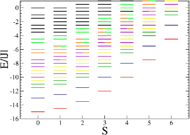
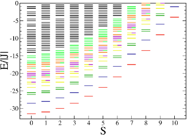
Figure 2: Part of the energy spectra of the rotational-band Hamiltonian for a cuboctahedron with twelve spins $s=1$ (left) and $s=3/2$ (right). Seven super-bands are colored.

Before discussing the results of our approximate diagonalization we would like to characterize the eigenbasis of $\!\hbox{}\mathop{\vphantom{H}\smash{H}}\limits_{\sim}\!{}_{\text{RB}}$. Figure 2 shows the low-lying part of the energy spectra of $\!\hbox{}\mathop{\vphantom{H}\smash{H}}\limits_{\sim}\!{}_{\text{RB}}$ for a cuboctahedron with $s=1$ and $s=3/2$ given by the rotational-band model. They exclusively consist of parabolas – so-called rotational bands. The eigenvalues $E_{\text{RB}}(S_{1},S_{2},S_{3},S)$ of $\!\hbox{}\mathop{\vphantom{H}\smash{H}}\limits_{\sim}\!{}_{\text{RB}}$ depend only on the spin quantum numbers of the sublattice spins $S_{n}$, with $n=1,2,3$, and of the total spin $S$. Corresponding eigenstates are trivial and analytically given as $|\alpha\,S_{1}\,S_{2}\,S_{3}\,S\,M\rangle$. The additional quantum number $\alpha$ refers to a set of intermediate spin quantum numbers which appears when coupling single spins $\!\hbox{}\mathop{\textbf{\vphantom{s}\smash{s}}}\limits_{\sim}\!{}_{i}$ of the same sublattice to the corresponding sublattice spins $\!\hbox{}\mathop{\textbf{\vphantom{S}\smash{S}}}\limits_{\sim}\!{}_{i}$ and further on coupling the sublattice spins to the total spin $\!\hbox{}\mathop{\textbf{\vphantom{S}\smash{S}}}\limits_{\sim}\hbox{}\!$. With regard to the set of intermediate spin quantum numbers $\alpha$ the number of all possible ways of constructing states characterized by fixed values of the sublattice and total spin quantum numbers determine the degeneracy of energy levels in the spectrum of the rotational-band Hamiltonian.

In the case of $s=1$ the lowest band in Fig. 2 is given by states $|\alpha\,S_{1}\,S_{2}\,S_{3}\,S\,M\rangle$ with sublattice spin quantum numbers $S_{1}=S_{2}=S_{3}=S_{\text{max}}=4\cdot 1=4$ while the second band is given by a deviation of one sublattice spin of 1, i.e. $|\alpha\,(S_{\text{max}}-1)\,S_{\text{max}}\,S_{\text{max}}\,S\,M\rangle$ and permutations thereof. The other bands can then be constructed by introducing additional deviations of the sublattice spin quantum numbers. The energy spectrum with $s=3/2$ shown in Fig. 2 can be constructed accordingly.

Additionally several energy levels in Fig. 2 are colored. This coloring refers to so-called super-bands. A super-band consists of those rotational bands for which the sum of sublattice spin quantum numbers is the same. In contrast to bipartite systems (see Ref. [6]) the spectrum of the rotational-band Hamiltonian for the cuboctahedron is much denser at low energies and only the first three super-bands are well separated from the others.

The classical ground state of the system plays the key role within the approximate diagonalization. The better the quantum mechanical system can be approximated by a classical picture of the ground state the more effectively the approximate diagonalization works, i.e. the faster the approximate energy eigenvalues converge towards the exact values. From a purely classical point of view the ground state of a cuboctahedron exhibits a three-sublattice structure and is infinitely degenerate since there coexist coplanar and non-coplanar vector orientations [32]. Here it should be emphasized that within the approximate diagonalization, i.e. within a quantum mechanical treatment, coplanarity of the classical ground state does not play a role, but the coloring of the classical ground state does, since there is a direct impact on the set of intermediate spin quantum numbers $\alpha$ in the rotational-band states $|\alpha\,S_{1}\,S_{2}\,S_{3}\,S\,M\rangle$ which are taken into account as basis states in the approximate diagonalization.

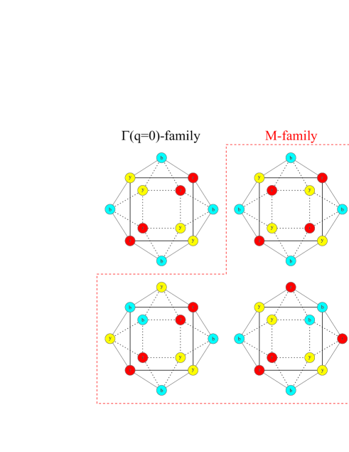
Figure 3: Families of the classical ground state of the cuboctahedron. Coloring of the $\Gamma(q=0)$-family (upper left). Coloring of the three equivalent states of the $M$-family (upper right and bottom). The drawing is a schematic planar projection. The labels correspond to y: yellow, r: red, and b: blue.

The classical ground state of the cuboctahedron exhibits 24 colorings of the spins which can be – by group theoretical considerations – decomposed into two families that are invariant under operation of the full point-group symmetry $O_{h}$ [19]. Following Ref. [19] these families will be denoted as $\Gamma(q=0)$-family and $M$-family. It has also been shown that those irreducible representations of $O_{h}$ which form the $\Gamma(q=0)$- and $M$-families are found in the low-lying part of the spectrum of the quantum cuboctahedron with half-integer spins $s=1/2,3/2,5/2$ [19]. Figure 3 shows the colorings of the different classical ground state families of the cuboctahedron. In a classical picture each color refers to a sublattice with all spins pointing into the same direction. The angle between classical spins belonging to different sublattices is $120^{\circ}$.

In order to calculate the approximate spectrum of the system one is now left with the construction of basis states of the form $|\alpha\,S_{1}\,S_{2}\,S_{3}\,S\,M\rangle$, i.e. quasi-classical states. Therefore spins belonging to the same sublattice have to be coupled to yield the total sublattice spins $\!\hbox{}\mathop{\textbf{\vphantom{S}\smash{S}}}\limits_{\sim}\!{}_{1}$, $\!\hbox{}\mathop{\textbf{\vphantom{S}\smash{S}}}\limits_{\sim}\!{}_{2}$ and $\!\hbox{}\mathop{\textbf{\vphantom{S}\smash{S}}}\limits_{\sim}\!{}_{3}$. Afterwards these total sublattice spins are coupled to the total spin $\!\hbox{}\mathop{\textbf{\vphantom{S}\smash{S}}}\limits_{\sim}\hbox{}\!$. The underlying coupling scheme is given by a classical ground state, i.e. a coloring from Fig. 3 and incorporated in the quantum number $\alpha$. In the following the resulting basis states will be labelled with respect to the classical reference state. To this end one has to distinguish between basis states of the form $|\gamma\,S_{1}\,S_{2}\,S_{3}\,S\,M\rangle_{\Gamma}$, $|\mu_{1}\,S_{1}\,S_{2}\,S_{3}\,S\,M\rangle_{M_{1}}$, $|\mu_{2}\,S_{1}\,S_{2}\,S_{3}\,S\,M\rangle_{M_{2}}$ and $|\mu_{3}\,S_{1}\,S_{2}\,S_{3}\,S\,M\rangle_{M_{3}}$. The notation of the set of intermediate quantum numbers and the subscript of the states now directly point to the classical ground state colorings, i.e. the underlying coupling scheme. It is important to note, that each of these four basis sets spans the same Hilbert space $\mathcal{H}(S,M)$.

In the case of the $M$-family three different colorings exist. When diagonalizing the Hamiltonian approximately while additionally using point-group symmetries one has to restrict to those symmetry groups where the symmetry operations do not alter the sublattice structure. A symmetry operation has no impact on the sublattice structure if the corresponding spin permutation results in recoloring of spins where all spins of a given sublattice maintain the same color, i.e. subscript (r: red, y: yellow, b: blue). For example an operation which leads to a cyclic permutation of colorings like

$$r\rightarrow y\rightarrow b\rightarrow r$$ (8)

has no impact on the sublattice structure.

While the sublattice structure of the $\Gamma(q=0)$-family is left invariant under all symmetry operations of $O_{h}$, the sublattice structure (i.e. coloring) of the $M$-family is not. In order to restore the sublattice invariance of the classical ground state belonging to the $M$-family the basis states for the approximate diagonalization can be constructed from a usually overcomplete set $M$ of basis states by an orthonormalization procedure. This set consists of rotational-band eigenstates from each coloring of the $M$-family, i.e. is given by

$$M=\left\{|\mu_{1}\,S_{1}\,S_{2}\,S_{3}\,S\,M\rangle^{i}_{M_{1}}\right\}+\left\{|\mu_{2}\,S_{1}\,S_{2}\,S_{3}\,S\,M\rangle^{i}_{M_{2}}\right\}+\left\{|\mu_{3}\,S_{1}\,S_{2}\,S_{3}\,S\,M\rangle^{i}_{M_{3}}\right\}\ ,$$ (9)

while the index $i$ is taking the values $1,\dots,n_{\text{red}}$. Here $n_{\text{red}}$ reflects the overall number of states contained in the incorporated rotational bands which is independent of the choice of the coupling scheme.

Since the underlying coupling scheme is different regarding the chosen coloring these states have to be converted into an – in general – arbitrary reference scheme $A$ before calculations can be performed. A transition between states belonging to different coupling schemes can be calculated using general recoupling coefficients [33, 34]. For the transition of a basis state $|\mu_{1}\,S\,M\rangle_{M_{1}}$ referring to a coloring $M_{1}$ of the $M$-family into the scheme $A$ one yields

$$|\alpha\,S\,M\rangle_{A}=\sum_{\alpha,S_{1},S_{2},S_{3}}{{}_{A}}\langle\alpha\,S\,M|\mu_{1}\,S\,M\rangle_{M_{1}}\,|\alpha\,S\,M\rangle_{A}\ ,$$ (10)

where the summation indices indicate that the summation is running over all valid combinations of values for the intermediate spin quantum numbers $\alpha$ as well as for the sublattice spin quantum numbers. The transitions between states of colorings $M_{2}$ and $M_{3}$ into the scheme $A$ can be obtained analogously.

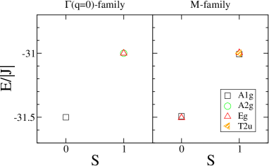
Figure 4: Classification by irreducible representations of $O_{h}$ of the quasi-classical states with lowest energies of the $\Gamma(q=0)$-family and $M$-family within $S=0$ and $S=1$ subspaces. The given energies refer to a diagonalization of the Heisenberg Hamiltonian exclusively within these quasi-classical states in the system with $s=3/2$.

Figure 4 shows the classification of the quasi-classical states with lowest energies within $S=0$ and $S=1$ subspaces according to irreducible representations of $O_{h}$. It corresponds to an approximate diagonalization of $\!\hbox{}\mathop{\vphantom{H}\smash{H}}\limits_{\sim}\!{}_{\text{Heisenberg}}$ using only a reduced basis set of states from the lowest rotational band in the system with $s=3/2$. Obviously the classification of the quasi-classical states is independent of the single spin quantum number $s$. Solely, the energies are changed when approximately diagonalizing the Hamiltonian of a system with different single spin quantum numbers. Based on a classical ground state belonging to the $\Gamma(q=0)$-family the states belong to the irreducible representations $A_{1g}$ ($S=0$) and $A_{2g}$, $E_{g}$ (S=1). Taking the $M$-family as a starting point for the construction of basis states the states belong to $A_{1g}$, $E_{g}$ (S=0) and $A_{1g}$, $E_{g}$, $T_{2u}$ (S=1) where the $T_{2u}$-state has apart from its intrinsic degeneration, i.e. the dimension of the irreducible representation $T_{2u}$, a twofold multiplicity.

The difference in the geometric properties of the lowest states of the chosen ground-state family, expressed by their decomposition into different irreducible representations, should directly lead to a convergence behaviour which depends on the choice of the underlying coloring. Since the approximate basis set contains energetically ordered states (from lowest to higher), low-lying states are expected to converge faster with growing number of basis states used for the approximate diagonalization [6].

3.1 Convergence of individual colorings

In Fig. 5 the approximate eigenvalues of a cuboctahedron with $s=1$ and $s=3/2$ in dependence on the number of incorporated bands within the $S=0$ subspaces are shown. As underlying classical ground states for each system the $\Gamma(q=0)$-family as well as one member of the $M$-family have been chosen. In every subfigure the last column refers to results from a complete diagonalization within $\mathcal{H}(S=0)$. Since the $\Gamma(q=0)$-family is invariant under $O_{h}$, the full point-group symmetry of a cuboctahedron ($O_{h}$) was used in order to classify the states. As mentioned before the individual members of the $M$-family are not invariant under $O_{h}$ but under $D_{2}$. Thus, in this case the $D_{2}$ point-group symmetry was applied.

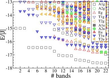
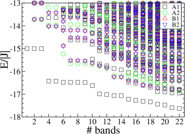
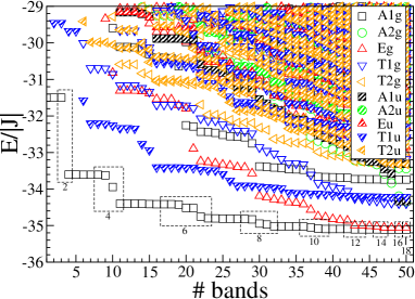
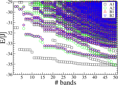
Figure 5: Low-lying energy spectra of a cuboctahedron with $s=1$ (upper row) and $s=3/2$ (lower row) within $S=0$ subspaces using an increasing number of bands (states). The underlying classical ground states belong to the $\Gamma(q=0)$-family (left) and to one coloring of the $M$-family (right) while $O_{h}$ (left) and $D_{2}$ (right) point-group symmetries were used in order to classify the states. The dashed boxes in the lower left figure indicate regions, i.e super-bands, in which the energy of the ground state is considerably lowered. The numbers refer to the number of magnons of the super-bands.

Looking at Fig. 5 it becomes apparent that the convergence is directly dependent on the choice of the underlying classical ground states. In agreement with theoretical expectations states which correspond to low-lying eigenstates of the rotational-band model converge faster than higher-lying states. Additionally, by comparing the spectra of $s=1$ and $s=3/2$ it can be seen that the ground state energy converges more rapidly with increasing single spin quantum number $s$. Nevertheless, apart from some states which exhibit a quite regular and fast convergence behaviour the convergence is – overall – rather poor. Especially the so-called low-lying singlet, which appears in the case of half-integer spins $s$ below the first triplet contributions, converges very slowly. This means that it is poorly approximated by one or a few eigenstates of the rotational-band Hamiltonian, but instead is a superposition of very many basis states.

One significant property which becomes evident when tracing single energy levels is that the convergence is stepwise – at least in the low-lying part of the spectra. Regions in which the ground state is considerably lowered are exemplarily marked with dashed boxes in the case of a cuboctahedron $s=3/2$ assuming a classical reference state of the $\Gamma(q=0)$-family. The numbers below the boxes refer to the number of magnons existing in the states of those rotational bands which are incorporated within the marked regions. Obviously the ground state energy is lowered whenever super-bands with an even number of magnons are incorporated in the approximate diagonalization. The observation of a stepwise convergence leads to a helpful additional approximation given by an approximate selection rule which is discussed below (see Sec. 3.4). It should be mentioned here that qualitatively the same convergence behaviour can be observed within subspaces of $S>0$. However, additional information cannot be extracted from graphical visualizations of the convergence in these subspaces, thus they will not be presented here.

3.2 Convergence of combined colorings

In order to improve the convergence of the energy levels in comparison to the behaviour shown in Fig. 5 the decomposition of the quasi-classical states in Fig. 4 directly leads to the starting point. Since the quasi-classical states, that result from different colorings, can be classified according to irreducible representations of $2A_{1g}$ and $E_{g}$, it is a straightforward task to use linear combinations of rotational-band eigenstates of the $\Gamma(q=0)$-family as well as of the $M$-family as basis states for the approximate diagonalization. The set of basis states results from an extension of $M$ in Eq. (9) to

$$\begin{split}G&=\left\{|\mu_{1}\,S_{1}\,S_{2}\,S_{3}\,S\,M\rangle^{i}_{M_{1}}\right\}+\left\{|\mu_{2}\,S_{1}\,S_{2}\,S_{3}\,S\,M\rangle^{i}_{M_{2}}\right\}\\ &\quad+\left\{|\mu_{3}\,S_{1}\,S_{2}\,S_{3}\,S\,M\rangle^{i}_{M_{3}}\right\}+\left\{|\gamma\,S_{1}\,S_{2}\,S_{3}\,S\,M\rangle^{i}_{\Gamma}\right\}\end{split}$$ (11)

and subsequent orthonormalization of the incorporated states.

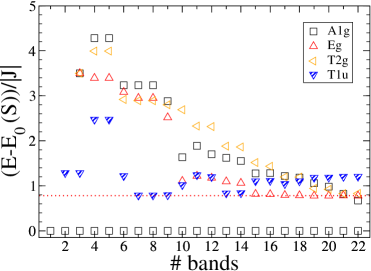
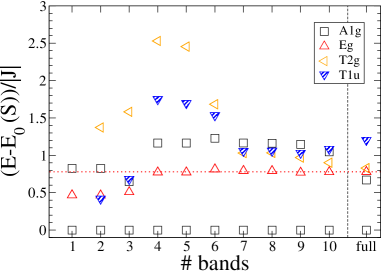
Figure 6: Energy difference to the ground state of selected low-lying energy levels of the cuboctahedron $s=1$ within $S=0$ subspace in dependence on the number of incorporated rotational bands. The reduced set of basis states is taken from rotational-band states of the $\Gamma(q=0)$-family only (left) and from linear combinations of states of all four colorings (right). The classification is according to $O_{h}$ point-group symmetry. The dotted red line refers to the exact difference to the $E_{g}$-state.

In Fig. 6 the energy difference between selected low-lying energy levels and the ground state of the system is displayed for a cuboctahedron $s=1$ within $S=0$ subspace. The difference is shown in dependence on the number of incorporated rotational bands. The last column refers in both subfigures to the exact values, taken from a complete diagonalization. The dotted red line indicates the energy difference to the $E_{g}$-state.

In the first case (left subfigure) only rotational-band states of the $\Gamma(q=0)$-family are taken into account for the approximate diagonalization. In the second case (right subfigure) linear combinations of states of all four colorings are used. The first noticeable difference is that when taking basis states of all colorings into account the low-lying levels start and remain in close proximity to their final (true) value. This is especially obvious when comparing the convergence of the lowest $A_{1g}$-state in both subfigures. The second difference is that when using linear combinations of states of all four colorings the convergence is smoother and more rapidly. This can be traced back to the fact that the different colorings contribute low-lying states of different irreducible representations which in the other families would only be available as high-lying states. Therefore, it is advantageous to use fewer bands but basis states of all classical colorings for the approximate diagonalization.

A short explanation might be appropriate in order to understand why the energy differences sometimes increase when taking more states into account. This is due to the fact that the ground state in such cases converges more rapidly than the excited states. Although all approximate eigenvalues improve on an absolute scale the differences get worse for a moment.

3.3 Results

In this section we like to present how good thermodynamic observables can be approximated. Figure 7 shows the specific heat $C(T,B)$ (left) and the magnetic susceptibility $dM/dB$ (right) for zero field $B=0$ of a cuboctahedron $s=3/2$. The energy spectrum of this system can be completely calculated using irreducible tensor operator technique in combination with a $D_{2}$ point-group symmetry [35]. In Fig. 7 the exactly calculated specific heat and the susceptibility are compared with results from an approximate diagonalization using only states of the lowest rotational band in each coloring in order to set up the basis. We also show how these observables look like if evaluated with only the lowest rotational band (L-band) of $\!\hbox{}\mathop{\vphantom{H}\smash{H}}\limits_{\sim}\!{}_{\text{RB}}$ (red colored energy levels in Fig. 2).

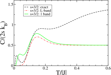
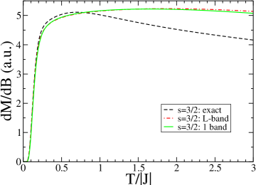
Figure 7: Comparison of approximate and exact specific heat $C(T,B)$ (left) and zero-field susceptibility $dM/dB$ (right) for a cuboctahedron $s=3/2$. The L-band refers to magnetic properties evaluated with the lowest band of the rotational-band Hamiltonian. For the approximate diagonalization only the states of the lowest rotational band but of each coloring are taken into account.

As one can see the low-temperature specific heat is very sensitive to the structure of low-lying levels. In the rotational-band model the lowest band (L-band) is gaped and describes a rotor. Therefore, the specific heat is suppressed at small temperatures and at higher temperatures approaches $3/2$ k_B. The approximate diagonalization, although only taking the lowest (L-band) states of all four coloring into account, achieves already an improvement for low-temperatures. The little Schottky-peak is the result of low-lying singlets and rearranging triplets. At higher temperatures this approximation displays the same behavior as the pure L-band which is expected since only L-band like states are incorporated.

In contrast to the specific heat which directly reflects the density of states within a certain energy interval the magnetic susceptibility reflects the density of magnetic states. To that end it is not surprising that the magnetic susceptibilities calculated from the approximate spectra do not differ considerably. Since the exact spectrum also possesses a rotational-band like behaviour at the lower edge the contributions from the approximate diagonalization and from the L-band reproduce the steep rise of the susceptibility for low temperatures very well. Obviously, the exact thermodynamical properties cannot be reproduced properly in the case of increasing temperature because the approximate spectra only contain a fraction of the energy levels of the full Hilbert space $\mathcal{H}$.

3.4 Approximate selection rule

As mentioned before (Sec. 3.1) the stepwise convergence behaviour leads to an approximate selection rule. Using this selection rule the computational effort when setting up the Hamilton matrices can be further reduced. In Fig. 5 it was shown that when diagonalizing in the $\Gamma(q=0)$-family, regions can be marked in which single energy levels are affected by taking into account additional rotational-band states. The same can be done for the $M$-family. As it was already mentioned, the marked regions coincide with the incorporation of rotational-band states belonging to the same super-band.

Looking at Fig. 5 the approximate energy eigenvalues of the ground state are lowered whenever states $|\gamma\,S_{1}\,S_{2}\,S_{3}\,S\,M\rangle$ are additionally included which belong to a super-band with an even number of magnons. Since the convergence behaviour is state-sensitive the energy of the lowest states belonging to the 3-dimensional irreducible representation $T_{1u}$, for example, is considerably lowered whenever super-bands with an odd number of magnons are included. This relation between the incorporation of super-bands and the immediate affection on the energies of certain approximate eigenstates can also be observed if the classical ground state belongs to the $M$-family.

As a result of the aforementioned observations a simple rule can be conjectured for low-lying energy levels $|S_{1,b}\,S_{2,b}\,S_{3,b}\,S\,M\rangle$. The matrix elements $\langle S_{1,a}\,S_{2,a}\,S_{3,a}\,S\,M|\!\hbox{}\mathop{\vphantom{H}\smash{H}}\limits_{\sim}\hbox{}\!|S_{1,b}\,S_{2,b}\,S_{3,b}\,S\,M\rangle$ connecting these states with other states $|S_{1,a}\,S_{2,a}\,S_{3,a}\,S\,M\rangle$ are one magnitude (or more) bigger than other matrix elements if

$$|n_{a}-n_{b}|\mod 2=0\ ,$$ (12)

where $n_{a}=\sum_{i=1}^{3}S_{i,\text{max}}-\sum_{i=1}^{3}S_{i,a}$ and $n_{b}$ (similarly evaluated), denote the number of magnons of the super-bands the states are belonging to. The Hamilton matrices approximately split up according to Eq. (12). Thus, simultaneously computation time is saved and the dimensionality of the problem is reduced.

4 Summary

In this paper an approximate diagonalization scheme was proposed and used in order to determine the energy spectra of geometrically frustrated spin systems. As an example the cuboctahedron was discussed. It was shown that the convergence is clearly dependent on the coloring of the underlying classical ground state, i.e on the coupling scheme. Therefore, the approximation can be improved by using an adapted set of basis states that originates from rotational-band states of all possible sublattice colorings. Furthermore, it was shown that the approximate diagonalization is useful in order to study the low-temperature thermodynamics of geometrically frustrated systems, even in its simplest form when only states from one rotational band within each coloring are taken into account.

Although the necessary calculations are rather involved, especially for huge frustrated systems, the approximate diagonalization can be a valuable method. Numerically the evaluation of recoupling coefficients constitutes the strongest challenge, i.e. calculations are rather limited by runtime than by available memory. However, recent developments show that highly parallelized program code or public resource computing can help to overcome this barrier.

References

- 1. D. Gatteschi, L. Pardi, Gazz. Chim. Ital. 123 (1993) 231
- 2. J. J. Borras-Almenar, J. M. Clemente-Juan, E. Coronado, B. S. Tsukerblat, Inorg. Chem. 38 (1999) 6081
- 3. O. Waldmann, Phys. Rev. B 61 (2000), 9 6138
- 4. I. G. Bostrem, A. S. Ovchinnikov, V. E. Sinitsyn, Theor. Math. Phys. 149 (2006) 1527
- 5. V. E. Sinitsyn, I. G. Bostrem, A. S. Ovchinnikov, J. Phys. A-Math. Theor. 40 (2007), 4 645
- 6. R. Schnalle, J. Schnack, Phys. Rev. B 79 (2009), 10 104419
- 7. S. R. White, Phys. Rev. B 48 (1993) 10345
- 8. M. Exler, J. Schnack, Phys. Rev. B 67 (2003) 094440
- 9. U. Schollwöck, Rev. Mod. Phys. 77 (2005) 259
- 10. C. Lanczos, J. Res. Nat. Bur. Stand. 45 (1950) 255
- 11. A. W. Sandvik, J. Kurkijärvi, Phys. Rev. B 43 (1991) 5950
- 12. A. W. Sandvik, Phys. Rev. B 59 (1999) R14157
- 13. L. Engelhardt, M. Luban, Phys. Rev. B 73 (2006) 054430
- 14. J. Schulenburg, A. Honecker, J. Schnack, J. Richter, H.-J. Schmidt, Phys. Rev. Lett. 88 (2002) 167207
- 15. C. Schröder, H.-J. Schmidt, J. Schnack, M. Luban, Phys. Rev. Lett. 94 (2005) 207203
- 16. R. Schmidt, J. Schnack, J. Richter, J. Magn. Magn. Mater. 295 (2005) 164
- 17. J. Schnack, R. Schmidt, J. Richter, Phys. Rev. B 76 (2007) 054413
- 18. V. O. Garlea, S. E. Nagler, J. L. Zarestky, C. Stassis, D. Vaknin, P. Kögerler, D. F. McMorrow, C. Niedermayer, D. A. Tennant, B. Lake, Y. Qiu, M. Exler, J. Schnack, M. Luban, Phys. Rev. B 73 (2006) 024414
- 19. I. Rousochatzakis, A. M. Läuchli, F. Mila, Phys. Rev. B 77 (2008) 094420
- 20. A. J. Blake, R. O. Gould, C. M. Grant, P. E. Y. Milne, S. Parsons, R. E. P. Winpenny, J. Chem. Soc.-Dalton Trans. (1997) 485
- 21. A. Müller, S. Sarkar, N. Shah, H. Bögge, M. Schmidtmann, S. Sarkar, P. Kögerler, B. Hauptfleisch, A. X. Trautwein, V. Schünemann, Angew. Chem., Int. Ed. 38 (1999) 3238
- 22. A. Müller, M. Luban, C. Schröder, R. Modler, P. Kögerler, M. Axenovich, J. Schnack, P. C. Canfield, S. Bud’ko, N. Harrison, Chem. Phys. Chem. 2 (2001) 517
- 23. M. Axenovich, M. Luban, Phys. Rev. B 63 (2001) 100407
- 24. C. Schröder, R. Prozorov, P. Kögerler, M. D. Vannette, X. Fang, M. Luban, Phys. Rev. B 77 (2008) 224409
- 25. J. Schnack, M. Luban, Phys. Rev. B 63 (2000) 014418
- 26. J. Schnack, M. Luban, R. Modler, Europhys. Lett. 56 (2001) 863
- 27. O. Waldmann, Phys. Rev. B 75 (2007) 012415
- 28. D. A. Varshalovich, A. N. Moskalev, V. K. Khersonskii, Quantum theory of angular momentum, World Scientific Publishing (1988)
- 29. M. Tinkham, Group theory and quantum mechanics, Dover Publications, New York (2003)
- 30. E. Weisstein, Mathworld, URL http://mathworld.wolfram.com
- 31. O. Waldmann, Phys. Rev. B 65 (2001)
- 32. H.-J. Schmidt, M. Luban, J. Phys. A: Math. Gen. 36 (2003) 6351
- 33. V. Fack, S. N. Pitre, J. van der Jeugt, Comp. Phys. Comm. 86 (1995) 105
- 34. V. Fack, S. N. Pitre, J. van der Jeugt, Comp. Phys. Comm. 101 (1997) 155
- 35. J. Schnack, R. Schnalle, Polyhedron, doi:10.1016/j.poly.2008.10.017