Generalized Holographic and Ricci Dark Energy Models

Abstract

In this paper, we consider generalized holographic and Ricci dark energy models where the energy densities are given as $\rho_{R}=3c^{2}M^{2}_{pl}Rf(H^{2}/R)$ and $\rho_{h}=3c^{2}M^{2}_{pl}H^{2}g(R/H^{2})$ respectively, here $f(x),g(y)$ are positive defined functions of dimensionless variables $H^{2}/R$ or $R/H^{2}$. It is interesting that holographic and Ricci dark energy densities are recovered or recovered interchangeably when the function $f(x)=g(y)\equiv 1$ or$f=g\equiv Id$ is taken respectively (for example $f(x),g(x)=1-\epsilon(1-x)$, $\epsilon=0\text{ or }1$ respectively). Also, when $f(x)\equiv xg(1/x)$ is taken, the Ricci and holographic dark energy models are equivalents to a generalized one. When the simple forms $f(x)=1-\epsilon(1-x)$ and $g(y)=1-\eta(1-y)$ are taken as examples, by using current cosmic observational data, generalized dark energy models are researched. As expected, in these cases, the results show that they are equivalent ($\epsilon=1-\eta=1.312$) and Ricci-like dark energy is more favored relative to the holographic one where the Hubble horizon was taken as an IR cut-off. And, the suggestive combination of holographic and Ricci dark energy components would be $1.312R-0.312H^{2}$ which is $2.312H^{2}+1.312\dot{H}$ in terms of $H^{2}$ and $\dot{H}$.

I Introduction

The observation of the Supernovae of type Ia ref:Riess98 ; ref:Perlmuter99 provides the evidence that the universe is undergoing accelerated expansion. Jointing the observations from Cosmic Background Radiation ref:Spergel03 ; ref:Spergel06 and SDSS ref:Tegmark1 ; ref:Tegmark2 , one concludes that the universe at present is dominated by $70\%$ exotic component, dubbed dark energy, which has negative pressure and pushes the universe to accelerated expansion. To explain the current accelerated expansion, many models are presented, such as cosmological constant, quintessence ref:quintessence1 ; ref:quintessence2 ; ref:quintessence3 ; ref:quintessence4 , phtantom ref:phantom , quintom ref:quintom and holographic dark energy ref:holo1 ; ref:holo2 etc. For recent reviews, please see ref:DEReview1 ; ref:DEReview2 ; ref:DEReview3 ; ref:DEReview4 ; ref:DEReview5 ; ref:DEReview6 .

In particular, a model named holographic dark energy has been discussed extensively ref:holo1 ; ref:holo2 ; ref:holo3 . The model is constructed by considering the holographic principle and some features of quantum gravity theory. According to the holographic principle, the number of degrees of freedom in a bounded system should be finite and has relations with the area of its boundary. By applying the principle to cosmology, one can obtain the upper bound of the entropy contained in the universe. For a system with size $L$ and UV cut-off $\Lambda$ without decaying into a black hole, it is required that the total energy in a region of size $L$ should not exceed the mass of a black hole of the same size, thus $L^{3}\rho_{\Lambda}\leq LM^{2}_{pl}$. The largest $L$ allowed is the one saturating this inequality, thus $\rho_{\Lambda}=3c^{2}M^{2}_{pl}L^{-2}$, where $c$ is a numerical constant and $M_{pl}$ is the reduced Planck Mass $M^{2}_{pl}=1/8\pi G$. It just means a duality between UV cut-off and IR cut-off. The UV cut-off is related to the vacuum energy, and IR cut-off is related to the large scale of the universe, for example Hubble horizon, event horizon or particle horizon as discussed by ref:holo1 ; ref:holo2 . In the paper ref:holo2 , the author takes the future event horizon

$$R_{eh}(a)=a\int^{\infty}_{t}\frac{dt^{{}^{\prime}}}{a(t^{{}^{\prime}})}=a\int^{\infty}_{a}\frac{da^{{}^{\prime}}}{Ha^{{}^{\prime}2}}$$ (1)

as the IR cut-off $L$. This horizon is the boundary of the volume a fixed observer may eventually observe. One is to formulate a theory regarding a fixed observer within this horizon. As pointed out in ref:holo2 , it can reveal the dynamic nature of the vacuum energy and provide a solution to the fine tuning and cosmic coincidence problem. In this model, the value of parameter $c$ determines the property of holographic dark energy. When $c>1$, $c=1$ and $c<1$, the holographic dark energy behaviors like quintessence, cosmological constant and phantom respectively. Unfortunately, when the Hubble horizon is taken as the role of IR cut-off, non-accelerated expansion universe can be achieved ref:holo1 ; ref:holo2 ; ref:BransDicke . However, the Hubble horizon is the most natural cosmological length scale, how to realize an accelerated expansion by using it as an IR cut-off will be interesting. One possibility is to generalize the holographic dark energy model. It will be one of the main points of this work.

Inspired by this principle, Gao, et. al. took the Ricci scalar as the IR cut-off and named it Ricci dark energy ref:Gao , $\rho_{R}=3c^{2}M^{2}_{pl}(\dot{H}+2H^{2}+k/a^{2})\propto R$. In that paper ref:Gao , it has shown that this model can avoid the causality problem and naturally solve the coincidence problem of dark energy. Interestingly, Cai, et. al. found out that the holographic Ricci dark energy had relations with the causal connection scale $R^{-2}_{CC}=Max(\dot{H}+2H^{2},-\dot{H})$ for a flat universe ref:CaiCC . Also, it was found that only the case where $R^{-2}_{CC}=\dot{H}+2H^{2}$ was taken as IR cut-off was consistent with the current cosmological observations when the vacuum density appears as an independently conserved energy component ref:CaiCC . The cosmic observational constraints to the Ricci dark energy model was studied in ref:HRDConstraint . In a manner, one can conclude that $H^{2}$ or $\dot{H}$ alone can not provide any late time accelerated expansion of the universe consistent with cosmic observations. But, their combination will do. It is the clue that generalized holographic models will be in the forms of their combinations.

As known, the holographic dark energy and Ricci dark energy both are candidates of dark energy can explain the late time accelerated expansion of our universe. It would be interesting to know which one is the most favored by current cosmic observational data. In general, we can use the comic observational data as constraints and implement Bayesian inference and model selection to test the goodness of models. However, we can test the goodness directly. It is the byproduct of this work. A generalized model can be designed to included holographic and Ricci dark energy by introduce a new parameter which balances holographic and Ricci dark energy model. The value of the new parameter determines this generalized model type: holographic, Ricci or a hybrid one. Of course, the best fit value of the model parameters is determined by cosmic data.

II Generalized holographic and Ricci dark energy

We consider a Friedmann-Robertson-Walker universe filled with cold dark matter and dark energy, here it will be holographic dark energy and Ricci dark energy. Its metric is written as

$$ds^{2}=-dt^{2}+a^{2}(t)\left(\frac{dr^{2}}{1-kr^{2}}+r^{2}d\theta^{2}+r^{2}\sin^{2}\theta d\phi^{2}\right),$$ (2)

where $k=1,0,-1$ for closed, flat and open geometries respectively. The Friedmann equation is

$$H^{2}=\frac{8\pi G}{3}\left(\rho_{m}+\rho_{de}\right)-\frac{k}{a^{2}},$$ (3)

where $H$ is the Hubble parameter, $\rho_{m}$ and $\rho_{de}$ denote the energy densities of cold dark matter and dark energy respectively.

In ref:holo1 ; ref:holo2 , when the Hubble horizon is taken as the IR cut-off, the holographic dark energy is written as

$$\rho_{h}=3c^{2}M^{2}_{pl}H^{2}.$$ (4)

Unfortunately, it can not give a current accelerated expansion universe ref:holo1 ; ref:holo2 ; ref:BransDicke in this case. In ref:Gao , Gao et. al. suggested the Ricci scalar can be taken as an IR cut-off, dubbed Ricci dark energy, which is proportional to the Ricci scalar

$$R=-6\left(\dot{H}+2H^{2}+\frac{k}{a^{2}}\right).$$ (5)

Then, it can be given as

$$\rho_{R}=3c^{2}M^{2}_{pl}R=3c^{2}M^{2}_{pl}\left(\dot{H}+2H^{2}+\frac{k}{a^{2}}\right),$$ (6)

where $R$ is the positive part of the Ricci scalar (5) and its coefficient is absorbed in $c^{2}$.

When the energy components have no interactions and the conservation equation

$$\dot{\rho}_{de}+3H(1+w_{de})\rho_{de}=0,$$ (7)

is respected, the equation of state of dark energy $w_{de}$ can be written as

$$w_{de}=-1-\frac{1}{3}\frac{d\ln\Omega_{de}}{dx}=-1+\frac{(1+z)}{3}\frac{d\ln\Omega_{de}}{dz}.$$ (8)

where $x=\ln a$, $\Omega_{de}=\rho_{de}/(3M^{2}_{pl}H^{2})$ is dimensionless energy density of dark energy, and the relation $1/a=1+z$ is used in above equation. The deceleration parameter $q(z)$ is defined as

$$q = -\frac{\ddot{a}}{aH^{2}}$$ (9)

$$= -\frac{\dot{H}+H^{2}}{H^{2}}$$

$$= -1+\frac{(1+z)}{2}\frac{d\ln H^{2}}{dz}$$

In this paper, we will consider a generalized versions of holographic and Ricci dark energy respectively. They are given in generalized forms

$$\rho_{GH} = 3c^{2}M^{2}_{pl}f\left(\frac{R}{H^{2}}\right)H^{2},$$ (10)

$$\rho_{GR} = 3c^{2}M^{2}_{pl}g\left(\frac{H^{2}}{R}\right)R,$$ (11)

where $f(x)$ and $g(y)$ are functions of the dimensionless variables $x=R/H^{2}$ and $y=H^{2}/R$ respectively. It is useful to write $R/H^{2}$ explicitly in the following form in a flat universe

$$\frac{R}{H^{2}} = \frac{\dot{H}+2H^{2}}{H^{2}}$$ (12)

$$= 2-\frac{(1+z)}{2}\frac{d\ln H^{2}}{dz}.$$

It can be easily seen that the holographic and Ricci dark energy models will be recovered when the function $f(x)=g(y)\equiv 1$. Also, when the function $f(x)=x$ and $g(y)=y$, the holographic and Ricci dark energy exchange each other. Clearly, the functions can be written as

$$f\left(\frac{R}{H^{2}}\right)=1-\epsilon\left(1-\frac{R}{H^{2}}\right),$$ (13)

$$g\left(\frac{H^{2}}{R}\right)=1-\eta\left(1-\frac{H^{2}}{R}\right),$$ (14)

where $\epsilon$ and $\eta$ are parameters. In this case, the above description can be interpreted as follows. When $\epsilon=0$ ($\eta=1$) or $\epsilon=1$($\eta=0$), the generalized energy density becomes holographic(Ricci) and Ricci(holographic) dark energy density respectively. Also, when the function has the relation $f(x)=xg(1/x)$ where the variable $x$ is $x=R/H^{2}$, the holographic and Ricci dark energy are equivalents to generalized ones. In the parameterized forms (13) and (14), the relation is $\epsilon=1-\eta$. Generally when $\epsilon\neq 0$($\eta\neq 0$) or $\epsilon\neq 1$($\eta\neq 1$), they are hybrid ones.

In the following sections, we will take Eq. (13) and Eq. (14) as simple examples to discuss the properties of the generalized dark energy models in a flat universe where the model parameters must be determined by cosmic observations. Once the best fit value of the parameters $\epsilon$ and $\eta$ was found, one can talk about which one is more favored by cosmic observations. If $\epsilon=0$ ($\eta=1$), the conclusion holographic dark energy is more favored. Or, one has the opposite conclusion. In fact, in these two forms, one expects the results would be that they are equivalent, i.e. $\epsilon=1-\eta$, because they are the combination in terms $\dot{H}$ and $H^{2}$. The parameters just give some balances between these terms. By fitting cosmic observations, the models’ orientation would be found: holographic- or Ricci-like.

III Generalized Holographic and Ricci Dark Energy Models

III.1 $f\left(\frac{R}{H^{2}}\right)=1-\epsilon\left(1-\frac{R}{H^{2}}\right)$ case

In this case, the Friedmann equation (3) can be rewritten as

$$H^{2} = \frac{1}{3M^{2}_{pl}}\left(\rho_{m}+\rho_{GH}\right)$$ (15)

$$= H^{2}\Omega_{m}+c^{2}\left[1-\epsilon\left(1-\frac{R}{H^{2}}\right)\right]H^{2},$$

where $\Omega_{m}=\rho_{m}/(3M^{2}_{pl}H^{2})$ is the dimensionless energy density of dark matter. The corresponding one of generalized holographic dark energy is

$$\Omega_{GH} = \frac{\rho_{GH}}{3M^{2}_{pl}H^{2}}$$ (16)

$$= c^{2}\left[1-\epsilon\left(1-\frac{R}{H^{2}}\right)\right]$$

$$= c^{2}\left(1+\epsilon-\frac{\epsilon(1+z)}{2}\frac{d\ln H^{2}}{dz}\right).$$

The Friedmann Eq. (15) can be rewritten as the differential equation of $H(z)$ with respect to redshift $z$

$$H^{2}\left\{1-c^{2}\left[1+\epsilon-\frac{\epsilon(1+z)}{2}\frac{d\ln H^{2}}{dz}\right]\right\}=H^{2}_{0}\Omega_{m0}(1+z)^{3},$$ (17)

which has the integration

$$H^{2}(z)=H_{0}^{2}\frac{2\Omega_{m0}(1+z)^{3}+C_{0}\left[2+c^{2}(\epsilon-2)\right](1+z)^{2-\frac{2}{c^{2}\epsilon}+\frac{2}{\epsilon}}}{2+c^{2}(\epsilon-2)},$$ (18)

where $C_{0}$ is an integral constant

$$C_{0}=\frac{\left[2+c^{2}(\epsilon-2)\right]-2\Omega_{m0}}{2+c^{2}(\epsilon-2)}.$$ (19)

In this case, the deceleration $q(z)$ is

$$q=\frac{1}{\epsilon}-\frac{\Omega_{GH}}{c^{2}\epsilon}.$$ (20)

III.2 $g\left(\frac{H^{2}}{R}\right)=1-\eta\left(1-\frac{H^{2}}{R}\right)$ case

In this case, the Friedmann equation (3) can be rewritten as

$$H^{2} = \frac{1}{3M^{2}_{pl}}\left(\rho_{m}+\rho_{GR}\right)$$ (21)

$$= H^{2}\Omega_{m}+c^{2}\left[1-\eta\left(1-\frac{H^{2}}{R}\right)\right]R.$$

The dimensionless energy density of generalized Ricci dark energy is

$$\Omega_{GR} = \frac{\rho_{GR}}{3M^{2}_{pl}H^{2}}$$ (22)

$$= c^{2}\left[1-\eta\left(1-\frac{H^{2}}{R}\right)\right]\frac{R}{H^{2}}$$

$$= c^{2}\left[(2-\eta)-(1-\eta)\frac{(1+z)}{2}\frac{d\ln H^{2}}{dz}\right].$$

The Friedmann Eq. (15) can be rewritten as the differential equation of $H(z)$ with respect to redshift $z$

$$H^{2}\left\{1-c^{2}\left[(2-\eta)-(1-\eta)\frac{(1+z)}{2}\frac{d\ln H^{2}}{dz}\right]\right\}=H^{2}_{0}\Omega_{m0}(1+z)^{3},$$ (23)

which has the solution

$$H^{2}(z)=H^{2}_{0}\frac{D_{0}\left[c^{2}(1+\eta)-2\right](1+z)^{\frac{2}{c^{2}(\eta-1)}+\frac{2(\eta-2)}{\eta-1}}-2\Omega_{m0}(1+z)^{3}}{c^{2}(1+\eta)-2},$$ (24)

where $C_{1}$ is an integral constant

$$D_{0}=\frac{\left[c^{2}(1+\eta)-2\right]+2\Omega_{m0}}{c^{2}(1+\eta)-2}.$$ (25)

The deceleration parameter is

$$q=\frac{1}{1-\eta}-\frac{\Omega_{GR}}{(1-\eta)c^{2}}.$$ (26)

One can immediately find out that they are equivalent when

$$\epsilon=1-\eta$$ (27)

from the comparison of Eq. (16) and Eq. (22). That can also be seen from the expression of deceleration parameter $q$.

III.3 Comparison and Discussion

It would be interesting to investigate how similar are the generalized holographic and Ricci dark energy models when the parameters are given by current cosmic observations. In the other words, we are going to understand which one is the most favored by confronting the cosmic observations. As shown in above subsections, they are equivalent when $\epsilon=1-\eta$ is respected. So, we can take one of them to investigate its properties. Here, we take the generalized holographic dark energy model as an example, the corresponding results of generalized Ricci one can be obtained by replacing $\eta=1-\epsilon$.

In Fig. 1, the 3D plots of $\Omega(z)$, $q(z)$ and $w(z)$ respectively with respect redshift $z$ and $\epsilon$ are presented in generalized holographic dark energy model where the value of parameter $c=0.6$, $\Omega_{m0}=0.27$ is adopted. From the figures, one can see that, in the generalized form of holographic dark energy model, a late time accelerated expansion of our universe is realized. That can not be obtained in holographic dark energy model where the Hubble horizon is taken as an IR cut-off. The reason may be that the Ricci component fills the missing gap or remedies the fake. By a further investigation, one would find out that the term $\dot{H}$ has the main effect. Here, we take this term with $H^{2}$, i.e. the Ricci scalar, as a whole. Also, one can find the properties of the generalized holographic dark energy is also determined by the parameter $\epsilon$ besides the parameter $c$. When $c$ and $z$ are fixed, with $\epsilon$ increasing in late time ($z<1$), the transition redshift from decelerated expansion to accelerated expansion is also increased, but decreasing of the EoS $w$ and $\Omega_{GH}$ of the generalized holographic dark energy. One would notice that in these plots the boundary values of parameter $\epsilon$ (i.e. $\epsilon=0$, or $\epsilon=1$ is not included in figures.). Also, one can find the corresponding results of generalized Ricci dark energy model by reflection of the plane $\epsilon=1/2$.

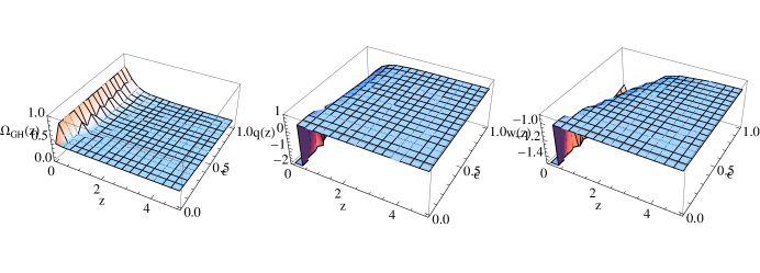
Figure 1: The 3D plots of $\Omega_{GH}(z)$, $q(z)$ and $w(z)$ in the case of generalized holographic dark energy models with redshift $z$ and $\epsilon$ where the values of parameters $c=0.6$, $H_{0}=72$ and $\Omega_{m0}=0.27$ are adopted. The corresponding results of generalized Ricci dark energy model can be obtained by reflection of the plane $\epsilon=1/2$.

Now, it is proper to present the constraint results by using cosmic observations: SN Ia, BAO and CMB shift parameter $R$, for the details please see Appendix A. After calculation, the results are listed in Tab. 1.

Models	$\chi^{2}_{min}$	$\Omega_{m0}(1\sigma)$	$c(1\sigma)$	$\epsilon(1\sigma)$	$\chi^{2}_{min}/dof$
GH	$316.855$	$0.325^{+0.039}_{-0.035}$	$0.579^{+0.030}_{-0.029}$	$1.312^{+0.353}_{-0.293}$	$1.035$

Table 1: The minimum values of $\chi^{2}$ and best fit values of the parameters of generalized holographic dark energy models. The corresponding results of generalized Ricci dark energy model can be obtained by reflection of the plane $\epsilon=1/2$. Here $dof$ denotes the model degrees of freedom.

From the best fit value of $\epsilon$ in Tab. 1, one can conclude that the generalized holographic and Ricci dark energy both incline to the Ricci side in the $\epsilon$ axis ($\epsilon\rightarrow 1$ in GH model, and $\epsilon\rightarrow 0$ in GR model) relative to the holographic side. Also, the interval to Ricci dark energy point is about $0.312$. It means the cosmic data favor a generalized dark energy model which is more Ricci-like. And, the suggestive combination of holographic and Ricci dark energy components would be $1.312R-0.312H^{2}$ which is $2.312H^{2}+1.312\dot{H}$ in terms of $H^{2}$ and $\dot{H}$.

The evolution curve of $q(z)$ with respect to redshift $z$ is plotted in Fig. 2. It is clear that, with these best fit values of model parameters, an late time accelerated expansion of our universe is obtained. The corresponding contour plots of model parameters can be found in Fig. 3. The transition redshift from decelerated expansion to accelerated expansion $z_{t}=0.507^{+0.512}_{-0.236}$ with $1\sigma$ region is found.

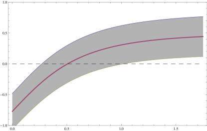
Figure 2: The evolution curve of $q(z)$ with redshift $z$ associated with $1\sigma$ region in the case of generalized holographic dark energy models where the best fit values of model parameters are adopted.

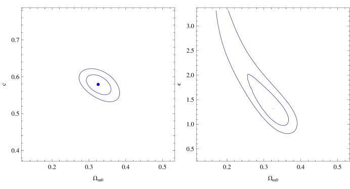
Figure 3: The contours in the planes of $\Omega_{m0}-c$ and $\Omega_{m0}-\epsilon$ with $1\sigma$ and $2\sigma$ regions. The dots denote the best fit values of model parameters. The corresponding results of generalized Ricci dark energy model can be obtained by reflection of the plane $\epsilon=1/2$.

IV Conclusion

In this paper, generalized holographic and Ricci dark energy models are presented, where the energy densities are given as $\rho_{R}=3c^{2}M^{2}_{pl}Rf(H^{2}/R)$ and $\rho_{h}=3c^{2}M^{2}_{pl}H^{2}g(R/H^{2})$ respectively, here $f(x),g(y)$ are positive defined functions of dimensionless variables $H^{2}/R$ or $R/H^{2}$. With these generalized forms, the holographic and Ricci dark energy densities are recovered or recovered interchangeably when the function $f(x)=g(y)\equiv 1$ or $f=g\equiv Id$ is taken respectively. As simple examples, we assume the forms of functions as $f(x)=1-\epsilon(1-x)$ and $g(y)=1-\eta(1-y)$. In these simple forms, one can immediately find that they are equivalent when $\epsilon=1-\eta$. It means the results of generalized holographic and Ricci dark energy are symmetric by reflection of the plane $\epsilon=1/2$. The best fit values of model parameters are obtained by using current cosmic observational data as constraints. The results show that an accelerated expansion of our universe can be obtained in generalized holographic dark energy model with contrast to holographic dark energy model where the Hubble horizon is taken as an IR cut-off. The generalized holographic and Ricci dark energy both incline to the Ricci side in the $\epsilon$ axis ($\epsilon\rightarrow 1$ in GH model, and $\eta\rightarrow 0$ the $\eta$ axis in GR model) relative to the holographic side. And, the interval to Ricci dark energy point is about $0.312$. It means the cosmic data favor a generalized dark energy model which is more Ricci-like. And, the suggestive combination of holographic and Ricci dark energy components would be $1.312R-0.312H^{2}$ which is $2.312H^{2}+1.312\dot{H}$ in terms of $H^{2}$ and $\dot{H}$. Of course, in phenomenological level, one can assume other forms of the generalized functions $f(x)$ and $g(y)$ to explore the possible properties of dark energy. We expect this kind of investigation can shed light on the research of dark energy.

Appendix A Cosmic Observations

A.1 SN Ia

We constrain the parameters with the Supernovae Cosmology Project (SCP) Union sample including $307$ SN Ia ref:SCP , which distributed over the redshift interval $0.015\leq z\leq 1.551$. Constraints from SN Ia can be obtained by fitting the distance modulus $\mu(z)$

$$\mu_{th}(z)=5\log_{10}(D_{L}(z))+\mu_{0},$$ (28)

where, $D_{L}(z)$ is the Hubble free luminosity distance $H_{0}d_{L}(z)/c$ and

$$d_{L}(z) = c(1+z)\int_{0}^{z}\frac{dz^{\prime}}{H(z^{\prime})}$$ (29)

$$\mu_{0} \equiv 42.38-5\log_{10}h,$$ (30)

where $H_{0}$ is the Hubble constant which is denoted in a re-normalized quantity $h$ defined as $H_{0}=100h~{}{\rm km~{}s}^{-1}{\rm Mpc}^{-1}$. The observed distance moduli $\mu_{obs}(z_{i})$ of SN Ia at $z_{i}$ is

$$\mu_{obs}(z_{i})=m_{obs}(z_{i})-M,$$ (31)

where $M$ is their absolute magnitudes.

For SN Ia dataset, the best fit values of parameters in a model can be determined by the likelihood analysis is based on the calculation of

$$\chi^{2}(p_{s},m_{0}) \equiv \sum_{SNIa}\frac{\left[\mu_{obs}(z_{i})-\mu_{th}(p_{s},z_{i})\right]^{2}}{\sigma_{i}^{2}}$$ (32)

$$= \sum_{SNIa}\frac{\left[5\log_{10}(D_{L}(p_{s},z_{i}))-m_{obs}(z_{i})+m_{0}\right]^{2}}{\sigma_{i}^{2}},$$

where $m_{0}\equiv\mu_{0}+M$ is a nuisance parameter (containing the absolute magnitude and $H_{0}$) that we analytically marginalize over ref:SNchi2 ,

$$\tilde{\chi}^{2}(p_{s})=-2\ln\int_{-\infty}^{+\infty}\exp\left[-\frac{1}{2}\chi^{2}(p_{s},m_{0})\right]dm_{0}\;,$$ (33)

to obtain

$$\tilde{\chi}^{2}=A-\frac{B^{2}}{C}+\ln\left(\frac{C}{2\pi}\right),$$ (34)

where

$$A=\sum_{SNIa}\frac{\left[5\log_{10}(D_{L}(p_{s},z_{i}))-m_{obs}(z_{i})\right]^{2}}{\sigma_{i}^{2}},$$ (35)

$$B=\sum_{SNIa}\frac{5\log_{10}(D_{L}(p_{s},z_{i})-m_{obs}(z_{i})}{\sigma_{i}^{2}},$$ (36)

$$C=\sum_{SNIa}\frac{1}{\sigma_{i}^{2}}\;.$$ (37)

The Eq. (32) has a minimum at the nuisance parameter value $m_{0}=B/C$. Sometimes, the expression

$$\chi^{2}_{SNIa}(p_{s},B/C)=A-(B^{2}/C)$$ (38)

is used instead of Eq. (34) to perform the likelihood analysis. They are equivalent, when the prior for $m_{0}$ is flat, as is implied in (33), and the errors $\sigma_{i}$ are model independent, what also is the case here.

To determine the best fit parameters for each model, we minimize $\chi^{2}(p_{s},B/C)$ which is equivalent to maximizing the likelihood

$${\cal{L}}(p_{s})\propto e^{-\chi^{2}(p_{s},B/C)/2}.$$ (39)

A.2 BAO

The BAO are detected in the clustering of the combined 2dFGRS and SDSS main galaxy samples, and measure the distance-redshift relation at $z=0.2$. BAO in the clustering of the SDSS luminous red galaxies measure the distance-redshift relation at $z=0.35$. The observed scale of the BAO calculated from these samples and from the combined sample are jointly analyzed using estimates of the correlated errors, to constrain the form of the distance measure $D_{V}(z)$ ref:Okumura2007 ; ref:Eisenstein05 ; ref:Percival

$$D_{V}(z)=\left[(1+z)^{2}D^{2}_{A}(z)\frac{cz}{H(z)}\right]^{1/3},$$ (40)

where $D_{A}(z)$ is the proper (not comoving) angular diameter distance which has the following relation with $d_{L}(z)$

$$D_{A}(z)=\frac{d_{L}(z)}{(1+z)^{2}}.$$ (41)

Matching the BAO to have the same measured scale at all redshifts then gives ref:Percival

$$D_{V}(0.35)/D_{V}(0.2)=1.812\pm 0.060.$$ (42)

Then, the $\chi^{2}_{BAO}(p_{s})$ is given as

$$\chi^{2}_{BAO}(p_{s})=\frac{\left[D_{V}(0.35)/D_{V}(0.2)-1.812\right]^{2}}{0.060^{2}}.$$ (43)

A.3 CMB shift Parameter R

The CMB shift parameter $R$ is given by ref:Bond1997

$$R(z_{\ast})=\sqrt{\Omega_{m}H^{2}_{0}}(1+z_{\ast})D_{A}(z_{\ast})/c$$ (44)

which is related to the second distance ratio $D_{A}(z_{\ast})H(z_{\ast})/c$ by a factor $\sqrt{1+z_{\ast}}$. Here the redshift $z_{\ast}$ (the decoupling epoch of photons) is obtained by using the fitting function Hu:1995uz

$$z_{\ast}=1048\left[1+0.00124(\Omega_{b}h^{2})^{-0.738}\right]\left[1+g_{1}(\Omega_{m}h^{2})^{g_{2}}\right],$$ (45)

where the functions $g_{1}$ and $g_{2}$ are given as

$$g_{1} = 0.0783(\Omega_{b}h^{2})^{-0.238}\left(1+39.5(\Omega_{b}h^{2})^{0.763}\right)^{-1},$$ (46)

$$g_{2} = 0.560\left(1+21.1(\Omega_{b}h^{2})^{1.81}\right)^{-1}.$$ (47)

The 5-year WMAP data of $R(z_{\ast})=1.710\pm 0.019$ ref:Komatsu2008 will be used as constraint from CMB, then the $\chi^{2}_{CMB}(p_{s})$ is given as

$$\chi^{2}_{CMB}(p_{s})=\frac{(R(z_{\ast})-1.710)^{2}}{0.019^{2}}.$$ (48)

For Gaussian distributed measurements, the likelihood function $L\propto e^{-\chi^{2}/2}$, where $\chi^{2}$ is

$$\chi^{2}=\chi^{2}_{SNIa}+\chi^{2}_{BAO}+\chi^{2}_{CMB},$$ (49)

where $\chi^{2}_{SNIa}$ is given in Eq. (38), $\chi^{2}_{BAO}$ is given in Eq. (43), $\chi^{2}_{CMB}$ is given in Eq. (48). In this paper, the central values of $\Omega_{b}h^{2}=0.02265\pm 0.00059$, $\Omega_{m}h^{2}=0.1369\pm 0.0037$ from 5-year WMAP results ref:Komatsu2008 and $H_{0}=72\pm{\rm 8kms^{-1}Mpc^{-1}}$ are adopted.

References

- (1) A.G. Riess, et al., Astron. J. 116 1009(1998) [astro-ph/9805201].
- (2) S. Perlmutter, et al., Astrophys. J. 517 565(1999) [astro-ph/9812133].
- (3) D.N. Spergel et.al., Astrophys. J. Supp. 148 175(2003) [astro-ph/0302209].
- (4) D.N. Spergel et al. 2006 [astro-ph/0603449].
- (5) M. Tegmark et al., Phys. Rev. D 69 (2004) 103501 [astro-ph/0310723].
- (6) M. Tegmark et al., Astrophys. J. 606 (2004) 702 [astro-ph/0310725].
- (7) I. Zlatev, L. Wang, and P.J. Steinhardt, Phys. Rev. Lett. 82 896(1999) [astro-ph/9807002].
- (8) P. J. Steinhardt, L. Wang, I. Zlatev, Phys. Rev. D59 123504(1999) [astro-ph/9812313].
- (9) M. S. Turner, Int. J. Mod. Phys. A 17S1 180(2002) [astro-ph/0202008].
- (10) V. Sahni, Class. Quant. Grav. 19 3435(2002) [astro-ph/0202076].
- (11) R. R. Caldwell, M. Kamionkowski, N. N. Weinberg, Phys. Rev. Lett. 91 071301(2003) [astro-ph/0302506].
- (12) B. Feng et al., Phys. Lett. B607 35(2005).
- (13) S. Weinberg, Rev. Mod. Phys. 61 1(1989).
- (14) V. Sahni and A. A. Starobinsky, Int. J. Mod. Phys. D 9 373(2000) [arXiv:astro-ph/9904398].
- (15) S. M. Carroll, Living Rev. Rel. 4 1(2001) [arXiv:astro-ph/0004075].
- (16) P. J. E. Peebles and B. Ratra, Rev. Mod. Phys. 75 559(2003) [arXiv:astro-ph/0207347].
- (17) T. Padmanabhan, Phys. Rept. 380 235(2003) [arXiv:hep-th/0212290].
- (18) E. J. Copeland, M. Sami and S. Tsujikawa, Int. J. Mod. Phys. D 15 1753(2006) [arXiv:hep-th/0603057].
- (19) S. D. H. Hsu, Phys. Lett. B594 13(2004) [arXiv:hep-th/0403052].
- (20) M. Li, Phys. Lett. B603 1(2004) [hep-th/0403127].
- (21) Q.G. Huang and M. Li, JCAP 0503, 001 (2005) [hep-th/0410095]; Q.G. Huang and M. Li, JCAP 0408, 013 (2004) [astro-ph/0404229]; B. Chen, M. Li and Y. Wang, Nucl. Phys. B 774, 256 (2007) [astro-ph/0611623]; J.F. Zhang, X. Zhang and H.Y. Liu, Eur. Phys. J.C 52 693(2007) [arXiv:0708.3121].
- (22) C. Gao, F. Wu, X. Chen, Y.G. Shen, Phys. Rev. D 79 043511(2009) [arXiv:0712.1394].
- (23) R. G. Cai, B. Hu and Y. Zhang, [arXiv:0812.4504].
- (24) L. Xu, W. Li, J. Lu, [arXiv:0810.4730]; X. Zhang, [arXiv:0901.2262]
- (25) L.X. Xu, W.B. Li, J.B. Lu, Eur. Phys. J. C 60 135 (2009).
- (26) M. Kowalski et al., Astrophys. J. 686, 749(2008) [arXiv:0804.4142].
- (27) S. Nesseris and L. Perivolaropoulos, Phys. Rev. D 72, 123519 (2005) [arXiv:astro-ph/0511040]; L. Perivolaropoulos, Phys. Rev. D 71, 063503 (2005) [arXiv:astro-ph/0412308]; S. Nesseris and L. Perivolaropoulos, JCAP 0702, 025 (2007) [arXiv:astro-ph/0612653]; E. Di Pietro and J. F. Claeskens, Mon. Not. Roy. Astron. Soc. 341, 1299 (2003) [arXiv:astro-ph/0207332].
- (28) T. Okumura, T. Matsubara, D. J. Eisenstein, I. Kayo, C. Hikage, A. S. Szalay and D. P. Schneider, ApJ 676, 889(2008) [arXiv:0711.3640]
- (29) D. J. Eisenstein, et al, Astrophys. J. 633, 560 (2005) [astro-ph/0501171].
- (30) W.J. Percival, et al, Mon. Not. Roy. Astron. Soc., 381, 1053(2007) [arXiv:0705.3323]
- (31) J. R. Bond, G. Efstathiou, and M. Tegmark, MNRAS 291 L33(1997).
- (32) W. Hu, N. Sugiyama, Astrophys. J. 471 542(1996) [astro-ph/9510117].
- (33) E. Komatsu, et.al., Astrophys. J. Suppl. 180, 330(2009) [arXiv:0803.0547].