Intrinsic Instability of Coronal Streamers

Abstract

Plasma blobs are observed to be weak density enhancements as radially-stretched structures emerging from the cusps of quiescent coronal streamers. In this paper, it is suggested that the formation of blobs is a consequence of an intrinsic instability of coronal streamers occurring at a very localized region around the cusp. The evolutionary process of the instability, as revealed in our calculations, can be described as follows, (1) through the localized cusp region where the field is too weak to sustain the confinement, plasmas expand and stretch the closed field lines radially outwards as a result of the freezing-in effect of plasma-magnetic field coupling; the expansion brings a strong velocity gradient into the slow wind regime providing the free energy necessary for the onset of the subsequent magnetohydrodynamic instability; (2) the instability manifests itself mainly as mixed streaming sausage-kink modes, the former results in pinches of elongated magnetic loops to provoke reconnections at one or multi locations to form blobs. Then, the streamer system returns to the configuration with a lower cusp point, subject to another cycle of the streamer instability. Although the instability is intrinsic, it does not lead to the loss of the closed magnetic flux, neither does it affect the overall feature of a streamer. The main properties of the modelled blobs, including their size, velocity profiles, density contrasts, and even their daily occurrence rate are in line with available observations.

1 INTRODUCTION

Coronal streamers are quasi-stationary large-scale structures observed during solar eclipses or with coronagraphs, they are believed to be the outcome of a complex magnetohydrodynamic (MHD) coupling between the hot expanding coronal plasmas and the large-scale confining magnetic field (e.g., Pneuman & Kopp, 1971; Koutchmy & Livshits, 1992). Many streamers remain visible over a period of up to several months. Nevertheless, various types of activities associated with coronal streamers are observed, including small-scale plasma blobs (Sheeley et al., 1997; Wang et al., 1998, 2000), streamer detachments with or without in/out pairs (Wang & Sheeley, 2006; Sheeley & Wang; 2007; Sheeley, Warren & Wang 2007), streamer blowout coronal mass ejections (CMEs) (Howard et al. 1985; Hundhausen 1993), and others (like streamer puffs (Bemporad et al. 2005), streamer deformations and deflections possibly induced by nearby coronal disturbances (e.g., Hundhausen 1987; Sheeley, Hakala, & Wang 2000)).

Among these activities, we are particularly interested in the formation of plasma blobs, which were discovered with the Large Angle Spectrometric Coronagraph (LASCO) onboard the Solar and Heliospheric Observatory (SOHO) (Brueckner et al. 1995), first reported by Sheeley et al. (1997). They manifest themselves as weak density enhancements emerging from the elongated tips of coronal streamers and confined to the narrow plasma sheet without causing any permanent disruption or dislocation of streamers. Since they are thought to flow passively along the bright plasma sheet and get dynamically coupled to the ambient plasmas, blobs are regarded as tracers of the ambient flow velocity with only slight contribution to the total slow wind mass flux. The estimated density inside the blobs is weakly enhanced over its surroundings by less than, say, 10 %. The sizes, when blobs are first observed, are about 1 R_⊙ in the radial direction and 0.1 R_⊙ in the transverse direction(corresponding to about 2^∘ in latitudinal extension). The blob speeds generally increase from 0 - 250 km s^-1 when first observed with LASCO C2 in the region 2 - 6 $R_{\odot}$ (solar radii) to about 250 - 450 km s^-1 in the region 20 -30 $R_{\odot}$ (Sheeley et al. 1997). It was shown by Wang et al. (1998) that the occurrence rate of blobs is about four per day along an edge-on streamer in the April of 1997, the quiet period of solar activities. During times of solar eruptions, the number, size and brightness of blobs generally increase (Wang et al. 2000).

Theoretical modelling of coronal streamers started early in the 1970s (e.g., Pneuman & Kopp, 1971). The classical model developed by Pneuman & Kopp treated the streamer as a magnetostatic structure in a bipolar configuration with a thin axisymmetric current sheet. The sheet extends from the tip of the closed streamer arcades to infinity, which separates the open field lines with opposite directions. Subsequent models presented similar morphological picture of streamers, many of them concentrate on the heating and acceleration of the corona and solar wind plasmas emphasizing the steady or quasi-steady feature of the streamer structure (e.g., Steinolfson et al., 1982; Wang et. al., 1993, 1998; Suess et al., 1999; Chen & Hu, 2001; Hu et al., 2003a; Suess & Nerney, 2006). Some authors did mention that it may be difficult to obtain an exact fully-converged steady state of the coronal streamer. For instance, Washimi et al. (1987) found that the modelled values of the velocity and density have a consistent temporal variation of about 1 $\%$ in magnitude per hour; Suess et al. (1996) demonstrated that the streamer is subject to slow and continuing evaporation till all the closed field lines are fully opened if heated with a volumetric heat source. Endeve et al. (2003, 2004), on the other hand, showed that coronal streamers can undergo eruptions if a specific heat source deposited inside the closed arcades is added to protons rather than electrons. It should be pointed out that the numerical resolution along the latitudinal direction in their studies is taken to be 2.77^∘ between adjacent grid points, which is even larger than the latitudinal size of the blobs observed by Sheeley et al, as introduced previously. Therefore, in these models it is impossible to resolve the blob structures as well as their formation process.

In Einaudi et al. (1999), the formation of blobs is simulated as magnetic islands resulting from the nonlinear development of the tearing mode instability along a hypothetical one dimensional Harris neutral sheet. The sheet is assumed to be embedded in a prescribed fluid wake, as a simplification of the realistic configuration associated with the streamer belt above the cusp. Refinements of this oversimplified incompressible model considered the effects of compressibility and inhomogeneous density distribution in relevance to the dense plasma sheet (Einaudi et al., 2001). By further considering the two-dimensional configuration with open and closed magnetic field lines and the specific cusp geometry, Lapenta & Knoll (2005) concluded that the reconnections forming the plasma blobs are driven by converging flows at the cusp region with reconnection rate mainly determined by the driving flows instead of resistivity, allowing their results to be extended to realistic coronal Lundquist numbers. However, their model is based on the Cartesian geometry with prescribed wake velocity field, and the imposed streamer morphology is not result from the self consistent dynamical equilibrium between the plasma expansion and magnetic confinement. In this paper, we present our theoretical endeavor in improving these relevant previous models for a better understanding of the formation of streamer blobs. The improvements are three-folds. Firstly, our calculations are conducted in the spherical geometry, which is somewhat more realistic compared with the planar cartesian geometry. Secondly, the streamer system in our model is self-consistently determined by the MHD coupling between plasmas and magnetic fields. Lastly, we take advantage of a much higher numerical resolution to better resolve the physical processes in the blob forming region. We show that the blobs are the consequence of an intrinsic instability of coronal streamers associated directly with the localized cusp region. In the following section we reveal the details of our theoretical model with initial and boundary conditions. The obtained solution for the streamer solar wind-blob system is shown in section 3. A brief summary of this article with discussion is provided in the last part of this article.

2 Theoretical models

Assuming the corona to be axisymmetric as in most previous studies, we solve the full-set two-dimensional and three-component (2.5d) ideal MHD equations in the spherical coordinate system ($r,\theta,\varphi$). A magnetic flux function $\psi(t,r,\theta)$ is introduced to express the magnetic field $\emph{{B}}(B_{r},B_{\theta},B_{\varphi})$ as

$$\emph{{B}}=\nabla\times({\psi\over r\sin\theta}\mathbf{\hat{\varphi}})+B_{\varphi}\mathbf{\hat{\varphi}}.$$

The deduced equations are given in Hu (2004) and are not to be repeated here. The equations are solved numerically in a domain of $R_{\odot}\leq r\leq 30R_{\odot}$ and $0\leq\theta\leq 90^{\circ}$, which is discretized into 300 $\times$ 632 grid points. Note that we also assume the system to be symmetric about the equator, thus the parameters in the other half of the latitudinal domain is derived from the obtained solution. The grid spacing increases according to a geometric series of a common ratio 1.015 along the radial direction from 0.005 $R_{\odot}$ at the solar surface to 0.437 $R_{\odot}$ at the top boundary. In the latitudinal direction, we first adopt a uniform mesh between $\theta=90^{\circ}$ to $\theta=30^{\circ}$ with grid spacing taken to be 0.1^∘, then we let the grid spacing increase according to a geometric series of a common ratio of 1.134 from $\theta=30^{\circ}$ to the pole. Such arrangement allows us to resolve the thin current sheets above the streamer cusps and the detailed dynamics of plasma blobs with high resolution. The multistep implicit scheme (MIS) developed by Hu (1989) is used to solve the MHD equations. The scheme has a relatively low numerical dissipation, which has been employed to deal with various issues in space physics, like the two-dimensional corona and solar wind solution driven by Alfveńic turbulence (Chen & Hu, 2001; Hu et al., 2003a, Li et al. 2004, 2006 ), and the flux rope catastrophe model for CMEs (Hu et al., 2003b; Chen et al., 2006, 2007). Since we are solving the equations under the framework of ideal MHD, any reconnections involved in the numerical solutions stem from numerical rather than physical resistivity. Therefore, the low dissipative feature of the adopted numerical scheme is critical to the issues we are concerned.

The heating and acceleration mechanisms of the corona and solar wind plasmas, which still remain unresolved at the present time, are approximated by using a polytropic process with the polytropic index taken to be $\gamma=1.05$. To start our modelling, the initial magnetic field is taken to be a quadrupolar one with the azimuthal component set to be zero and the magnetic flux function given by Antiochos et al. (1999) as follows,

$$\psi(r,\theta)={\psi_{c}}\{{\sin^{2}\theta R_{\odot}\over r}+{(3+5\cos 2\theta)\sin^{2}\theta{R_{\odot}}^{3}\over 2r^{3}}\}$$

where $\psi_{c}={\psi_{0}B_{p}\over{10B_{0}}}$, the unit of magnetic field strength $B_{0}=0.833$ Gauss, the unit of magnetic flux function $\psi_{0}=4.04\times 10^{13}$ Wb, and the magnetic field strength at the pole $B_{p}$ is taken to be 8 Gauss. It is known that a neutral point exists in this potential field at $r_{N}=\sqrt{3}R_{\odot}$ along the equator with $\psi=0.3697\psi_{0}$. The reasons we adopt this specific topology, rather than the often used bipolar topology for this study are given as follows. First, the triple-streamer system is more realistic, especially when one models the corona at high solar activity. As a matter of fact, even at solar minimum, the corona is often observed to have a few rather than one-single well-defined streamers. Second, this allows us, in future development of the model, to extend the break-out CME model originally proposed by Antiochos et al. (1999) to the case including the effect of the solar wind. Further elaboration concerning the relevance to the CME modelling will be given in the last section. Third, by focusing on the dynamics of the side streamer which is fully located inside the calculation domain, we avoid the influence of the symmetric boundary conditions along the equator.

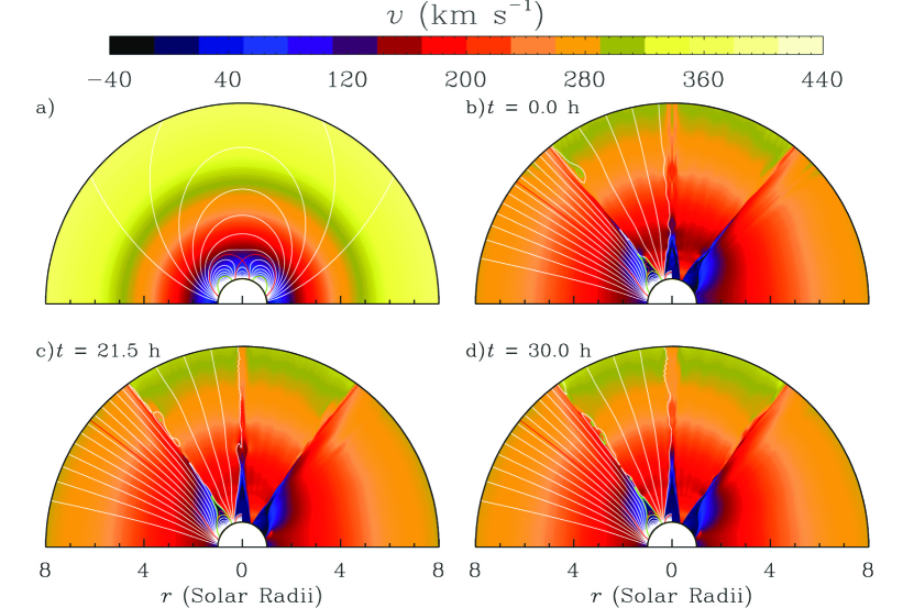
Figure 1: Magnetic field lines superposed by the contour map of the two-dimensional distribution of the radial velocity field from 1 to 10 $R_{\odot}$. The field lines are represented by the contours of the magnetic flux function with the contour level separated by $\psi=0.05\psi_{0}$. Panel a) is for the initial quadrupolar field and solar wind velocity, b) - d) depict the calculated conditions at various instants. The separatrix associated with the original quadrupolar field ($\psi=0.3697\psi_{0}$) is shown in red curves. The three lines in green, red, and yellow colors in the blob region are given by $\psi=0.655,0.66$, and $0.665\psi_{0}$, referred to as line A, B, and C in the text. To show features in the contour map of the radial velocity, the magnetic field lines are omitted in one of the hemispheres in b) - d). [The long-term dynamical evolution (in 2 days from t=0 to 48 hours) of the triple-streamer solar wind blob system is shown in an mpeg animation in the electronic edition of the Journal.]

In Figure 1a we show the magnetic field lines of the initial quadrupolar field from 1 to 10 $R_{\odot}$, represented by the contours of the magnetic flux function with the contour level separated by $\psi=0.05\psi_{0}$. On the solar surface, the magnetic flux function first increases from 0 at the pole to 1.2 $\psi_{0}$ near the center of the side arcade, and then decreases again to 0 at the equator. The separatrix in the initial quadrupolar field specified by $\psi=0.3697\psi_{0}$ is shown as red curves. It is easy to see that the initial magnetic field consists of four flux system including the central arcade system straddling the equator, two side ones centered at $\theta=45^{\circ}$ and $135^{\circ}$, and an overlying polar flux system. As will be clearly illustrated in the following section, the initial magnetic topology is subject to significant change by the plasma-field coupling process.

At the lower boundary ($r=1R_{\odot}$), the magnetic flux function $\psi$ is fixed to the values given by the above equation, the plasma temperature is set to be constant at 2 MK. The density, which is assumed to be dependent on the latitude, is 10⁸ cm^-3 and 1.5$\times 10^{8}$ cm^-3 in the region $\theta=[0,30^{\circ}]$ and $[60^{\circ},90^{\circ}]$, respectively, and increases linearly from $\theta=30^{\circ}$ to $60^{\circ}$. Note that although the assumption of an inhomogeneous density distribution at the lower boundary results in a discontinuous latitudinal pressure gradient there, essentially similar physical processes occur when assuming a homogeneous density distribution, as revealed by calculations not presented here. The radial and latitudinal velocity components at the lower boundary are obtained by the mass conservation and the parallel condition given by $\emph{{V}}\parallel\emph{{B}}$. The azimuthal components of the velocity and magnetic field are set to be zero. All parameters are extrapolated to get the conditions at the top boundary, and symmetric conditions are employed at both the equator and the pole. We are aware that the boundary conditions are somewhat arbitrarily chosen in order to obtain a solution with reasonable streamer structures and solar wind parameters, they are still in line with available observational constraints. The initial solar wind condition is an educated guess which does not have impacts on the final large scale converged numerical solution as confirmed by the calculations. For example, the radial velocity is set to be a function of radial distance increasing monotonically from 1.1 km/s at the bottom to 400 km/s at the top. The contour map of the two-dimensional distribution of the prescribed radial velocity field is depicted in Figure 1a. With the initial and boundary conditions described above, the coupling between the plasma dynamical motion and the coronal magnetic field is self-consistently taken care of using our numerical code. The calculation finally converges to a quasi-steady solution featured by a triple-streamer, slow solar winds emanating from the poles and between the closed arcades, and plasma blobs continuously released from the streamer tips, as will be depicted in the following section.

3 The triple-streamer solar wind-blob system

To save computation time required for the solution to converge, the calculations were first conducted in the same domain but with much less grid points in the latitudinal direction than described in the last section till a quasi-steady state was reached, which was redistributed to the present denser grid points. In the case with lower resolution the number of grid points in the latitudinal direction is taken to be 150 with grid spacing uniformly distributed between $\theta=90^{\circ}$ to $\theta=30^{\circ}$ with a resolution of 0.5^∘, and increasing according to a geometric series of a common ratio of 1.046 from $\theta=30^{\circ}$ to the pole. The number and distribution of grid points in the radial direction are taken to be the same in all calculations. The obtained solution was then allowed to evolve self-consistently for a long time, e.g., for a few hundred hours. The magnetic field lines with contour map of the radial velocity field of a solution at an arbitrarily-selected instant are shown in Figure 1b. For the purpose of illustration, the time of this solution is set to be zero (i.e., t=0). As mentioned previously and clearly indicated by Figures 1a and 1b, the original quadrupolar topology of the magnetic field is reshaped significantly by the presence of the solar wind plasmas. The most apparent change is the formation of the triple-streamer system with solar wind plasmas streaming into interplanetary space from both polar regions and the narrow regions between the central and the side streamers. In the outer part of the original side arcade system a few field lines are opened by the solar wind plasmas, while a few other field lines reconnect at the current sheet along the equator and close back resulting in an increase of the closed magnetic flux of the central arcades. This causes the disappearance of the original neutral line at the intersection of the red curves ($\psi=0.3697\psi_{0}$) in Figure 1a, and has a profound impact on the break-out model for CMEs proposed by Antiochos et al. (1999) based on the field topology shown in Figure 1a. We will return to this point in the last section. The field lines with the same value of $\psi$ are also plotted in Figure 1b to 1d for comparisons.

In Figures 1c and 1d we illustrate the magnetic field topology and the radial velocity field at t=21.5 and 30 hours, respectively, so as to indicate the long-term evolution of the dynamical streamers. To show features in the contour map of the radial velocity, the magnetic field lines are omitted in one of the hemispheres in Figure 1b to 1d. An accompanying mpeg animation of the temporal evolution of the solution from t=0 to 48 hours with frames separated by 10 minutes in time interval is provided with the online version of this paper. The solution at t=21.5 hours will be re-shown in the following figure to reveal the streamer dynamics in more detail. Note that the equator is taken as a boundary with symmetric conditions, we are aware that such treatment certainly has impacts on the dynamics associated with the central streamer. We will revisit this issue again as we proceed. Therefore, in this article we concentrate only on the dynamics atop the side streamer. Yet, the modelling results in the central streamer region can still be used for the purpose of comparison.

It is obvious from Figure 1 and the online animation that the streamer is in a constant state of motion with small magnetic/plasma islands released continuously from the elongated tips of the side streamers, despite the long-term large-scale stability of the overall morphology. As indicated by the solutions, generally speaking, the islands have no regular shapes, the latitudinal width is about 0.1 to 0.2 $R_{\odot}$, and the radial length about 1 to 1.5 $R_{\odot}$ when the islands are first separated from the main streamer. The plasma inside the islands is denser than the surrounding solar wind plasmas. For example, for the solution at t=23.5 hours, which will be further illustrated in the following figures, the center of an island just released is located at about 3.6 $R_{\odot}$. The density at this distance is about 1.5 $\times 10^{6}$ cm^-3 inside the island, and 1.4 $\times 10^{6}$ cm^-3 in the nearby equatorward solar wind and about 1.0 $\times 10^{6}$ cm^-3 in the nearby polarward wind. The quantities of our modelled magnetic islands are basically consistent with the LASCO observations for streamer blobs reported by Sheeley at al. (1997) and Wang et al. (1998), and summarized in the introduction part of this article. We therefore regard them as streamer blobs hereinafter. The white field line delineating the outer boundary of streamer blobs in Figure 1 and the online animation is given by $\psi=0.65\psi_{0}$. To reveal more details of the blob dynamics, we also plot three more adjacent magnetic field lines with $\psi=0.655,0.66,0.665\psi_{0}$ in green, red, and yellow colors, referred to as line A, B, and C, respectively. It can be seen that among them line C shows no apparent motion during the process, indicating that the blob formation involves only the localized cusp and current sheet region. The process does not result in the loss of the closed magnetic flux of the side streamer.

As seen from the online animation, daughter blobs are found to form as a result of the breakup of a longer mother blob. After the formation, blobs change their length and shape continuously during the outward propagation. They usually get wider as a result of the relaxation of magnetic tension of reconnected field lines. It is also observed that two approaching blobs with differential speeds may get merged into one blob structure at certain distances. After checking the animated solution carefully, we get an average occurrence rate of about 6-8 blobs per day. Note that this estimate has excluded the blobs that are possibly too small to be measurable with current coronagraphs. The propagation velocity profiles of blobs, as estimated from our numerical results, are found to basically follow that of the surrounding solar wind plasmas. These modelling features can be regarded as in a remarkable agreement with available observations at the quiet time of solar activity considering the simplicity of our model.

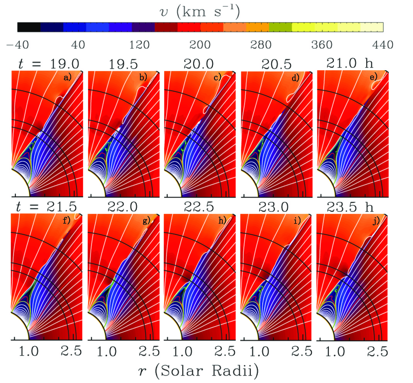
Figure 2: Ten image frames of the side streamer part cropped from the corresponding global versions of images, spanning from t=19 to t= 23.5 hours. The frames are separated by 30 minutes in time interval with time increasing from left to right and top to bottom. The three black arcs are centered at the sun with radius being 2.35, 2.6, and 3.6 $R_{\odot}$. [This figure is available as part of the mpeg animation in the electronic edition of the Journal.]

As clearly seen from the velocity maps depicted in Figure 1b to 1d, there exists apparent velocity shear on the two sides of the blob forming region. It is natural to surmise that the formation of blobs is related to the presence of the strong velocity shears that are capable of driving various modes of streaming MHD instabilities. To get deeper insights of how blobs are formed, in Figure 2 we show 10 image frames spanning from t=19 to t= 23.5 hours, separated by 30 minutes in time interval with time increasing from left to right and top to bottom. All images are the side streamer part cropped from their corresponding global versions which are similar as that shown in Figure 1. For example, Figure 2f is corresponding to Figure 1c (t=21.5 hours). From Figure 2a, we see that a narrow long blob (referred to as blob I) is just formed from magnetic reconnection and starts its outward propagation. About 4 to 4.5 hours later, another blob is released from the same streamer (referred to as blob II) following the trend of its predecessor. Therefore, the images collected in Figure 2 delineate a complete cycle of blob formation of typical configuration. Below we shall describe the evolutionary process and physical interpretation of the formation of blob II by illustrations with Figures 2 and 3.

For a visual guide, in Figure 2 we add three black arcs centered at the sun with radius being 2.35, 2.6, and 3.6 $R_{\odot}$. We see from Figure 2a that the streamer cusp is reformed at a lower distance of about 2.6 $R_{\odot}$ upon the disconnection of blob I. The magnetic field at the newly reformed cusp region is apparently too weak to sustain the confinement of the plasmas at coronal temperature, the plasmas expand and stretch the freezing-in closed field lines radially outwards. Consequently the streamer tip elongates as clearly seen from the upper panels of Figure 2. After a continuing expansion for about 2 to 2.5 hours line A (in white color with $\psi=0.655\psi_{0}$) starts to pinch at its middle part. It is apparent that the physics accounting for the pinching of field lines drives the following reconnection shown in Figure 2i and 2g. To check the physical conditions at the initial stage of the line pinch, in the left panel of Figure 3 we plot the radial components of velocity and magnetic field vectors ($v_{r}$ and $B_{r}$) together with the Alfvén speed ($v_{A}$) for the solution shown in Figure 2f (t=21.5 hours) as a function of co-latitude ($\lambda=90{{}^{\circ}}-\theta$). The profiles are plotted at the 3 heliocentric distances used for the visual guide, i.e., 2.35 (solid), 2.6 (dotted), and 3.6 (dashed) $R_{\odot}$.

From the $v_{r}$ profile, we see that there exists a strong velocity jump between the surrounding solar wind plasmas along open field lines and that inside the elongated closed loops reaching up to nearly 150 km s^-1 at 2 to 3 solar radii. In the shear region the magnetic field changes its direction, and the overall strength is relatively weak compared to that in the surrounding solar wind regimes. Note that $B_{r}$ at 2.6 $R_{\odot}$ (the dotted line) changes its polarity 3 times in the shear region. This feature is an aftermath of blob I, and will be interpreted later together with the physical origin of the small concave morphology of lines A and B at the streamer tips upon the formation of blobs I and II. The Alfvén speed reaches the minimum value inside the velocity shear, as a result of the weak magnetic field there. Generally speaking, from 2.35 to 3.6 $R_{\odot}$ the Alfvén speed is less than 75 km s^-1 in the solar wind flowing between the central and the side streamers, much higher in the polar wind regime, and less than 50 km s^-1 inside the velocity shear region.

Velocity shears in plasmas can generate Kelvin-Helmholtz (KH) instabilities (e.g. Miura & Pritchett 1982). The physical configuration as shown in Figure 3a to 3c is somewhat similar to that studied previously by, e.g., Lee, Wang & Wei (1988) for streaming instabilities (more widely known as KH instability), although they investigated the situation with velocity maximum located inside the current sheet region, on the contrary to our situation. Such discrepancy can be easily reconciled if one applies a coordinate transformation from their configuration into a moving reference system with an appropriate velocity, e.g., the maximum velocity in their configuration. With the transformation, the real part of the frequency is doppler-shifted, and the instability criteria, eigenmode profiles, and growth rate remain unaffected. Using their linear model of streaming instability, Lee et al. (1988) determined the eigenmode profiles and critical conditions (see Equations (41) and (42) in their article) for both the sausage and the kink modes. To take advantage of the deduced conditions, we need to specify the Alfvén speed in the shear region and in the surrounding plasmas, the number density, the wave number, and the half width of the shear region. Referring to the parameter profiles plotted in Figure 3a to 3c, we assume an Alfvén speed to be 20 km s^-1 inside and 75 km s^-1 outside the shear region, the half width of the shear to be 0.05 $R_{\odot}$, and the density to be distributed homogeneously. After simple calculations with Lee et al.’s critical conditions, we find that in the hypothetical configuration for the specified wave length of 1 $R_{\odot}$ (typical length of a blob), the velocity gradient should be no less than 158 km s^-1 for the sausage mode and 100 km s^-1 for the kink mode to take place. By checking Figure 3a, we find that the total velocity jump presented in our solution at the time field line A starts to pinch can indeed reach up to 150 to 160 km s^-1. This implies that both the sausage and the kink modes of streaming instabilities can occur in our configuration. We emphasize that the above estimate is rather rough and carried out with a much simpler configuration than that represented by Figure 3a to 3c. It is well known that the sausage mode results in the variation of the current sheet thickness to form a sausagelike configuration, and the kink mode produces a wavy structure keeping the current sheet thickness relatively constant. By checking the online animation again, it is apparent that both the sausagelike and wavy structures are present in the blob forming region. Thus, the occurrence of the mixed sausage-kink mode instability in our solutions is actually self-evident. On the other hand, the symmetric boundary conditions adopted at the equator effectively prohibit the growth of the kink mode. Hence only streaming sausage mode can be observed atop the central streamer.

From the above text, we propose that the pinch of field lines is caused by the streaming sausage mode instability. The instability, ideal in nature, is unable to produce reconnections. Yet, with the nonlinear growth of the instability, the distance decreases and the current density increases consistently in between the elongating field lines till whatever dissipation mechanism sets in to cause reconnection. Therefore, we suggest that the reconnections accounting for the blob separations are driven by the nonlinear development of the sausage mode. The reconnections could be caused by the well-known resistive tearing mode instability, or simple magnetic diffusion process across the narrow layer with enhanced current density. To determine the exact process acting in this highly-nonlinear MHD simulation, one needs to consider a more sophisticated and physical model of resistivity and a finer numerical resolution to reduce the numerical resistivity as low as possible. This is generally rather robust and computationally expensive, and remains unresolved in the current study. As apparently seen from the multi-blob formation in our numerical solution, reconnections can take place simultaneously at various locations. The wavelength of the sausage mode is reflected by the length of the blob just formed, which is about 1.0 $R_{\odot}$ to 1.5 $R_{\odot}$. The upper limit of the growth time of the sausage mode can be estimated by measuring the time span from a field line starts to pinch to a blob is finally released, which is about 2 to 3 hours according to Figure 2e to 2j.

The sausage mode instability is energized by the free energy associated with the velocity shear present in the blob forming region. To see how velocity shear evolves after the formation of a blob, in the right panels of Figure 3 (3d - 3f) we plot the latitudinal profiles for the solution shown in Figure 2j (t=23.5 hours) at the same three distances as used in the left panels. From Figure 2j, it can be seen that the break point of the streamer is located at about 2.6 $R_{\odot}$, the profiles at this distance are plotted as dotted lines. The velocity shear almost vanishes crossing the streamer break point, as the aftermath of the sausage-mode instability. It can be seen from the solid lines plotted in both Figures 3a and 3d, strong velocity shear is always present at a lower distance of 2.35 $R_{\odot}$. Such velocity shear is along the streamer leg between the open and closed magnetic field lines, where the local magnetic field is relatively strong and a KH instability is unable to develop. In the following 2 to 3 hours of continuous streamer elongation after t=23.5 hours, the strong velocity shear is brought into the slow wind regime again where the field strength gets lower so that the critical conditions for streaming instabilities can be satisfied.

Similar to the profile for 2.6 $R_{\odot}$ plotted in Figure 3b, the radial magnetic field at about 2.35 $R_{\odot}$ in Figure 3e also presents a triple change of polarity. This feature can be straightforwardly explained by the concave-inward morphology of line B and its adjacent lines not plotted here. The formation of the concave-inward morphology can be interpreted as follows. The causes are different for different field lines. For the field line that is just broken by reconnections, like line B (in red color) in Figure 2i, the morphology is a result of the relaxation of intensified magnetic tension of the over-stretched field lines upon reconnections. For the field line overlying the lines just reconnected, like line A in Figures 2a and 2i, the morphology is a result of magnetic pressure gradient force which points inwards as a result of the rapid shrinking of those lines just reconnected (like line B).

As a summary of this section, the formation of streamer blobs can be regarded as consisting of two successive processes, one is the plasma-magnetic field expansion through the localized cusp region where the field is too weak to sustain plasma confinement, the other is the onset of the sausage mode instability that finally triggers magnetic reconnections producing separated plasma blobs. The former process brings strong velocity shear into the slow wind regime, and provides required free energy for the following streaming instabilities. By checking the time frames collected in Figure 2 for a complete cycle of the formation of a typical blob, we find that generally the streaming sausage mode instability sets in after the expansion continues for about 2 to 2.5 hours. The expansion continues till the nonlinear development of the instability finally breaks the elongated loops, which takes another 2 to 3 hours, producing a streamer blob and a ‘new’ coronal streamer with a lower cusp. The whole process originates from the peculiar magnetic topological feature at the cusp region intrinsically associated with a coronal streamer. We therefore term the described process as intrinsic instability of coronal streamers. Although the instability is intrinsic, it does not lead to the loss of the closed magnetic flux, so it does not influence the overall feature of a streamer.

4 Conclusions and discussion

It is well known that a coronal streamer system is resulted from the dynamical equilibrium between plasma expansion and magnetic confinement. Despite the overall long-term stability of the morphology, it is suggested that the streamer is subject to an intrinsic instability originating from the peculiar magnetic topological feature at the cusp region. The whole process of the instability consists of two successive processes, one is the plasma-magnetic field expansion through the localized cusp region where the field is too weak to maintain plasma confinement, the continuing expansion brings strong velocity shear into the slow wind regime providing free energy necessary for the onset of a streaming sausage mode instability which causes pinches of magnetic field lines and drives reconnections at the pinching points to form separated magnetic blobs.

Although our recent two-dimensional models for the corona and solar wind have considered the role of Alfvén waves in the formation of the bipolar coronal streamer and the solar wind as a two-fluid and two-state plasmas (Chen & Hu, 2001; Hu et al., 2003a), in this paper we still take advantage of the polytropic assumption of the heat transport process for simplicity. These previous streamer and solar wind models were aimed at investigating the heating and acceleration of the corona and solar wind plasmas emphasizing the large-scale stability of the corona streamers rather than the detailed dynamics of blobs. To do this, a certain amount of numerical dissipation was applied to stabilize the calculations. As a drawback of this treatment, the dynamical processes associated with blob formations have been largely smoothed out in these previous models. Note that although no explicit heating is applied to the plasma in the present model, a polytropic index of $\gamma=1.05$ and a temperature of 2 MK at the inner boundary results in the high-temperature coronal plasma with a nature to expand. In a future extension to the present model, one may let $\gamma={5\over 3}$ and employ a more realistic energy balance equation to model the plasma heating process. This will change the details of the plasma-magnetic coupling process, and thus the streamer morphology as well as the solar wind and blob properties. However, we believe that the overall physics of blob formation suggested above, namely, the instabilities are essentially due to the presence of an intrinsic streamer cusp with the dynamics determined by the elongation of the freezing-in plasma-magnetic arcades, which brings the relatively slow confined plasmas into the solar wind regime resulting in enough velocity shear to trigger the streaming sausage mode instability, remains largely unaffected.

In the study by Lapenta & Knoll (2005), blobs are interpreted as a result of reconnections along open current sheet structure beyond the streamer cusps. This can be seen by comparing their Figure 6a and Figure 6d (also 7a and 7c, 7d and 7f). At the end of their case calculation there is an apparent increase of the closed-flux inside the streamer. The increase can be more than 50-100% of the original total closed flux contained by their streamer if the magnetic flux function along adjacent field lines plotted in their figures is equally separated. Thus, the streamer itself will grow significantly and continuously after blobs form one by one. Although the magnetic field is not directly observable in the corona, this shall be inconsistent with observations which indicate that blobs have only minor contributions to the solar wind plasmas resulting in no dislocation or disruption of the streamer. In our study, blobs are thought to form along elongating closed arcades below the streamer cusp. The closed streamer flux is not influenced by the blob formation in any significant way. Furthermore, according to our calculations, reconnections occur in the region where the field lines are almost parallel to each other, rather than in the region where flows/field lines converge most, therefore, the idea of converging-flow driven reconnection to form blobs, as proposed by Lapenta & Knoll, seems to be inappropriate at least in our more realistic streamer configurations.

Our calculations started from the quadrupolar magnetic field with a neutral point high in the corona, exactly in the form provided by Antiochos et al. (1999) in their break out model for CMEs. They investigated the dynamical response of the closed arcades to foot point shearing motions. One key point of the breakout model lies in the presence of a multipolar pre-eruptive field with a magnetic null (or neutral point) high in the corona. With the shearing motions, the high magnetic null gradually extends into a current sheet structure that manages to survive for a certain time in the corona plasmas. Through magnetic forces the current sheet structure serves as a major agent confining the increasing free magnetic energy of the sheared central arcades. Eruptions take place when the thickness of the current sheet structure eventually decreases to trigger the fast break-out reconnections through either physical or numerical resistivity. The original breakout model did not take into account the effect of expanding plasmas on the global magnetic field morphology. Such effect is non-negligible especially at the heights where the original breakout model is concerned and at the null neighborhood with very weak magnetic field strength. The consequence of this effect has been clearly illustrated by the calculations presented in this article, especially, by comparisons of the upper panels of our first figure. We found that the original morphology of the quadrupolar magnetic field is re-shaped into a triple-streamer configuration with its neutral point blown away by the solar wind, indicating the critical impact of the solar wind plasmas on the coronal field topology that causes the failure of the breakout mechanism within the framework of our modelling. In future studies, we are going to construct a CME model based on the triple-streamer solar wind state obtained in this paper using the ideal catastrophe mechanism of magnetic flux rope system as the triggering and major energizing mechanism for eruptions (see, e.g., Chen et al., 2006, 2007).

Figure 3: The radial components of velocity and magnetic field vectors ($v_{r}$ and $B_{r}$) together with the Alfvén speed ($v_{A}$) for the solutions at t = 21.5 hours left) and 23.5 hours (right). The parameters are shown as a function of co-latitude ($\lambda=90^{\circ}-\theta$) for 3 heliocentric distances of 2.35 (solid), 2.6 (dotted), and 3.6 (dashed) $R_{\odot}$.

References

- (1) Antiochos, S. K., DeVore, C. R., & Klimchuk, J. A. 1999, ApJ, 510, 485
- Bemporad et al. (2005) Bemporad, A. et al. 2005, ApJ, 635, L189
- Bruecknet et al. (2007) Bruecknet, G. E., et al. 1995, Sol. Phys., 162, 357
- Chenhu (2001) Chen, Y., & Hu, Y. Q. 2001, Sol. Phys., 199, 371
- Chen et al. (2007) Chen, Y., Hu, Y. Q., & Sun, S. J. 2007, ApJ, 665, 1421
- Chen et al. (2006) Chen, Y., Li, G. Q., & Hu, Y. Q. 2006, ApJ, 649, 1093
- Endeve et al. (2003) Endeve, E., Leer, E., & Holzer, T. E. 2003, ApJ, 589, 1040
- Endeve et al. (2004) Endeve, E., Holzer, T. E., & Leer, E. 2004, ApJ, 603, 307
- (9) Einaudi, G., Boncinelli, P., Dahlburg, R. B., & Karpen, J. T. 1999, 104(A1), 521
- (10) Einaudi, G., Chibbaro, S., Dahlburg, R. B., & Velli, M. 2001, ApJ, 547, 1167
- How (1985) Howard, R. A., et al. 1985, J. Geophys. Res., 90, 8173
- Hu (1989) Hu, Y. Q. 1989, J. Comput. Phys. 84, 441
- (13) Hu, Y. Q. 2004, ApJ, 607, 1032
- (14) Hu, Y. Q., Habbal, S. R., Chen, Y., & Li, X. 2003a, 108(A10), 1377, doi:10.1029/2002JA009776
- (15) Hu, Y. Q., Li, G. Q., & Xing X. Y. 2003b, J. Geophys. Res., 108(A2), 1072, doi:10.1029/2002JA009419
- Hundhausen, (1987) Hundhausen, A. J. 1987, Proceedings of the 6th International Solar Wind Conference, edited by Pizzo V. J., Holzer T., and Sime D. G., p181
- Hundhausen, (1993) Hundhausen, A. J. 1993, J. Geophys. Res., 98, 13177
- Kou, (1992) Koutchmy, S., & Livshits, M. 1992, Spa. Sci. Revs., 61 (3-4), 393
- lapenta, (05) Lapenta, G., & Knoll, D. A. 2005, ApJ, 624, 1049
- Lee et al., (1988) Lee, L. C., Wang, S., & Wei, C. Q. 1988, J. Geophys. Res., 93(A7), 7354
- li, (2004) Li, B., Li, X., Habbal, S.R., & Hu, Y.Q. 2004, JGR, 109, 10.1029/2003JA010313, 2004.
- li, (2006) Li, B., Li, X., & Labrosse, N. 2006, JGR, 111, A08106, doi:10.1029/2005JA01130, 2006
- miura, (1982) Miura, A., & Prichett, P.L. 1982, JGR, 87, 7431
- Pnuuman, Kopp, (1971) Pneuman, G. W., & Kopp, R. A. 1971, Sol. Phys., 18, 258
- Sheeley et al. (2000) Sheeley, N. R., Hakala W. N., & Wang Y. M. 2000, JGR, 105(A3), 5081
- Sheeley, Wang (2007) Sheeley, N. R. & Wang Y. M. 2007, ApJ, 655, 1142
- Sheeley et al. (2007) Sheeley, N. R., Warren H. P., & Wang Y. M. 2007, ApJ, 671, 926
- Sheeley et al. (1997) Sheeley, N. R., et al. 1997, ApJ, 484, 472
- Steinolfson et al. (1982) Steinolfson, R. S., Suess, S. T., & Wu S. T. 1982, ApJ, 255, 730
- Suess, Nerney (2006) Suess, S. T., & Nerney, S. F. 2006, Geophys. Res. L., 33(10), CiteID L10104
- Suess et al. (1996) Suess, S. T., Wang, A. H., and Wu, S. T. 1996, J. Geophys. Res., 101, 19,957.
- Suess et al. (1999) Suess, S. T., Wang, A. H., Wu, S. T., & Nerney, S. F., 1999, Space Sci. Rev., 87, 323
- Wang et al. (1993) Wang, A. H., Wu, S. T., Suess, S. T., & Poletto, G. 1993, Sol. Phys., 147, 55
- Wang et al. (1998) Wang, A. H., Wu, S. T., Suess, S. T., & Poletto, G. 1998, J. Geophys. Res. 103, 1913
- Wang et al. (1988) Wang, S., Lee, L. C., & Wei C. Q., 1988, Phys. Fluids, 31 (6), 1544
- Wang et al. (1998) Wang, Y. M., et al. 1998, ApJ, 498, L165
- Wang et al. (2000) Wang, Y. M., et al. 2000, JGR, 105(A11), 25133
- Wang et al. (2006) Wang ,Y. M. & Sheeley, Jr. N. R. 2006, ApJ, 650, 1172
- (39) Washimi, H., Yoshino, Y., & Ogino, T. 1987, Geophys. Res. Lett., 14, 487