On Some Stratifications of Affine Deligne-Lusztig Varieties for $SL_{3}$

Abstract.

Let $L:=\bar{k}((\epsilon))$, where $k$ is a finite field with $q$ elements and $\epsilon$ is an indeterminate, and let $\sigma$ be the Frobenius automorphism. Let $G$ be a split connected reductive group over the fixed field of $\sigma$ in $L$, and let $I$ be the Iwahori subgroup of $G(L)$ associated to a given Borel subgroup of $G$. Let $\widetilde{W}$ be the extended affine Weyl group of $G$. Given $x\in\widetilde{W}$ and $b\in G(L)$, we have some subgroup of $G(L)$ that acts on the affine Deligne-Lusztig variety $X_{x}(b)=\{gI\in G(L)/I:g^{-1}b\sigma(g)\in IxI\}$ and hence a representation of this subgroup on the Borel-Moore homology of the variety. This dissertation investigates this representation for certain $b$ in the cases when $G=SL_{2}$ and $G=SL_{3}$.

1. Introduction

Let $k$ be a finite field with $q$ elements and let $\bar{k}$ be an algebraic closure of $k$. Let $\sigma:\bar{k}\to\bar{k}$ be the Frobenius morphism $\sigma(a)=a^{q}$. Let $L:=\bar{k}((\epsilon))$, where $\epsilon$ is an indeterminate, and extend $\sigma$ to $L$ by setting $\sigma(\epsilon)=\epsilon$. Denote the valuation ring $\bar{k}[[\epsilon]]$ of $L$ by $\mathfrak{o}_{L}$. Let $F:=k((\epsilon))$ and denote $k[[\epsilon]]\subset\mathfrak{o}_{L}$ by $\mathfrak{o}_{F}$.

Let $G$ be a split connected reductive group over $F$. Let $A$ be a split maximal torus of $G$. Let $W$ denote the Weyl group of $A$ in $G$ and let $\widetilde{W}=W\ltimes X_{*}(A)$ denote the extended affine Weyl group. Fix a Borel subgroup $B$ containing $A$, so that $B=AU$, with $U$ unipotent, and let $I$ denote the corresponding Iwahori subgroup of $G(L)$. Then we have the Bruhat decomposition of $G(L)$ into double cosets $IxI$, where $x\in\widetilde{W}$. Let $X=G(L)/I$. Let $U_{w}=w^{-1}U(L)w$, so that $U_{1}=U(L)$.

If $b\in G(L)$, then the $\sigma$-conjugacy class of $b$ is $\{g^{-1}b\sigma(g):g\in G(L)\}$. For every $x\in\widetilde{W}$ we define (following [2]) the affine Deligne-Lusztig variety $X_{x}(b)=\{gI\in X\,:\,g^{-1}b\sigma(g)\in IxI\}$. Note that if $b_{1}$ and $b_{2}$ are in the same $\sigma$-conjugacy class, with $b_{1}=h^{-1}b_{2}\sigma(h)$, then the varieties $X_{x}(b_{1})$ and $X_{x}(b_{2})$ are isomorphic, with the isomorphism $X_{x}(b_{1})\to X_{x}(b_{2})$ given by the translation $gI\to hgI$.

Consider the subgroup $H<G(L)$ consisting of elements $h$ such that $h^{-1}b\sigma(h)=b$. Elements of $H$ then act on the variety $X_{x}(b)$ by left-multiplication. This action induces a representation of $H$ on the Borel-Moore homology of $X_{x}(b)$.

Our goal is to study this representation when $G=SL_{n}$, $n=2,3$ and $b$ is a diagonal matrix whose nonzero entries have the form $\epsilon^{\nu_{i}}$, where $\nu_{i}\neq\nu_{j}$ if $i\neq j$. We will refer to such a $b$ as $\epsilon^{\nu}$, where $\nu=(\nu_{1},\nu_{2},\ldots,\nu_{n})$. In general, we will use $\epsilon^{\mu}$ to refer to an element of $G(L)$ which has the form

$$\begin{pmatrix}\epsilon^{\mu_{1}}&0&\cdots&0\\ 0&\epsilon^{\mu_{2}}&\cdots&0\\ \vdots&\vdots&\ddots&\vdots\\ 0&0&\cdots&\epsilon^{\mu_{n}}\end{pmatrix}.$$

For our choice of $b$, the subgroup $H$ acting on $X_{x}(\epsilon^{\nu})$ is $A(F)=\mathbb{Z}^{n-1}\times A(\mathfrak{o}_{F})$. We will show that the subgroup $A(\mathfrak{o}_{F})$ acts trivially on the Borel-Moore homology of $X_{x}(\epsilon^{\nu})$, and therefore the representation of $A(F)$ factors through the representation of $\mathbb{Z}^{n-1}$. This last representation is induced by the action which is given by $(i_{1},\ldots,i_{n-1})\cdot gI=\epsilon^{(i_{1},\ldots,i_{n-1},-i_{1}-\ldots-i_{n-1})}gI$, and corresponds to permutation of the homology spaces of disjoint closed subsets of $X_{x}(\epsilon^{\nu})$.

In order to study these representations, we will develop, in Section 2.1, a method that, given $g\in G(L)$ and $x\in\widetilde{W}$, gives necessary and sufficient conditions for $g$ to be in $IxI$ in terms of the valuations of the determinants of the minors of $g$ (including the $1\times 1$ minors). We will also develop, in Section 2.2, a method that, given $g\in G(L)$ and $w\in\widetilde{W}$, produces the element $x\in\widetilde{W}$ such that $g\in w^{-1}U_{1}wxI$. Then in Sections 2.3 and 2.4 we will prove some general theorems applicable to $SL_{n}$ and $GL_{n}$ which we will later use for $SL_{3}$.

For the case $G=SL_{2}$, we will show that the representation of $A(\mathfrak{o}_{F})$ on the Borel-Moore homology of $X_{x}(\epsilon^{\nu})$ is trivial by showing that not only do we have a left-multiplication action of $A(\mathfrak{o}_{F})$ on $X_{x}(\epsilon^{\nu})$ but that we also have a left-multiplication action of the bigger group $A(\mathfrak{o}_{L})$ on $X_{x}(\epsilon^{\nu})$. Since $A(\mathfrak{o}_{L})$ is connected, the action of $A(\mathfrak{o}_{F})$ on the homology of $X_{x}(\epsilon^{\nu})$ must be trivial. This will be done in Chapter 3.

For the case $G=SL_{3}$, this approach would work in most cases, but there are some situations in which $A(\mathfrak{o}_{L})$ does not act on $X_{x}(\epsilon^{\nu})$ by left-multiplication. The approach we will take for $SL_{3}$ will be to decompose $X_{x}(\epsilon^{\nu})$ into a union of disjoint closed subsets, each of which is preserved by $A(\mathfrak{o}_{F})$, to produce a stratification of each of these closed subsets into strata preserved by $A(\mathfrak{o}_{F})$, and finally to extend the action of $A(\mathfrak{o}_{F})$ on each stratum to an action of $A(\mathfrak{o}_{L})$. We will then argue that this means that the representation of $A(\mathfrak{o}_{F})$ on the Borel-Moore homology of each of the disjoint closed subsets is trivial. This will be done in Chapter 4.

The author would like to thank Robert Kottwitz for his suggestion of a research direction and many useful conversations.

2. Preliminaries

In this chapter we develop some techniques that will be used later. Throughout the chapter, $G$ is $SL_{n}$ or $GL_{n}$ for any $n\geq 2$. Let $K=G(\mathfrak{o}_{L})$.

Let $V=L^{n}$. If we fix a basis for $V$, we may view elements of $G(L)$ as $n\times n$ matrices with elements in $L$. Fix the basis for $V$ such that the elements of $A(L)$ are diagonal matrices and the elements of $B(L)$ are upper triangular; call this basis $\{v_{1},\ldots,v_{n}\}$. Then with respect to this basis, an element $M$ of $I$ has the form

(1) $$M_{ij}\in\begin{cases}\mathfrak{o}_{L}^{\times}&\text{if $i=j$}\\ \mathfrak{o}_{L}&\text{if $i<j$}\\ \epsilon\mathfrak{o}_{L}&\text{if $i>j$}\end{cases}.$$

From this point on, we always work in this basis, and identify elements of $G(L)$ with matrices, and elements of $\widetilde{W}$ with their unique representatives which are monomial matrices whose nonzero entries have the form $\epsilon^{k}$, $k$ an integer.

2.1. Determining the Iwahori Double-Coset for a Given Element of $G(L)$

Let $M\in G(L)$ and $x\in X_{x}(\epsilon^{\nu})$. We want to give necessary and sufficient conditions for $M$ to be in $IxI$. We will show that these conditions can be expressed in terms of conditions on the valuations of the determinants of minors of $M$.

To prove this, we first reduce the problem to that of looking at valuations of elements by considering $\bigwedge^{m}\!V$ for $m=1,\ldots,n$. Any ordered $m$-tuple of distinct integers from $1$ to $n$ determines a vector in $\bigwedge^{m}\!V$—given the $m$-tuple $(i_{1},\ldots,i_{m})$ we get the vector $v_{i_{1}}\wedge\cdots\wedge v_{i_{m}}$. The vectors corresponding to the set of increasing $m$-tuples give a basis for $\bigwedge^{m}\!V$. We pick an order for this basis by lexicographically ordering the increasing $m$-tuples, and from this point on this is the basis we use for $\bigwedge^{m}\!V$.

Given any matrix $M\in G(L)$ we define the matrix $\bigwedge^{m}\!M$ by requiring that

$$\left(\bigwedge^{m}\!M\right)(v_{i_{1}}\wedge\cdots\wedge v_{i_{m}})=(Mv_{i_{1}})\wedge\cdots\wedge(Mv_{i_{m}}).$$

Lemma 2.1.1.

If $M$ has the form given in (1), then so does $\bigwedge^{m}\!M$ for any $m$.

Proof.

An entry of $\bigwedge^{m}\!M$ is the determinant of an $m\times m$ minor of M. To be more precise, if we number the increasing $m$-tuples of integers between 1 and $n$, ordered lexicographically, from 1 to $\binom{n}{m}$ then $(\bigwedge^{m}\!M)_{ij}$ is the determinant of the minor of $M$ which consists of entries in rows given by the $i$-th $m$-tuple and columns given by the $j$-th $m$-tuple. Since all entries of $M$ are in $\mathfrak{o}_{L}$, it is clear that any such determinant will be in $\mathfrak{o}_{L}$.

If $i=j$, then the two $m$-tuples are identical and if we reduce all entries in the minor modulo $\epsilon\mathfrak{o}_{L}$ we will get an upper triangular matrix with elements of $\bar{k}^{\times}$ on the diagonal. Its determinant will be an element of $\bar{k}^{\times}$. But that means that the determinant of our original minor is in $\mathfrak{o}_{L}^{\times}$, as desired.

Finally, if $i>j$ we need to show that the determinant of the minor is in $\epsilon\mathfrak{o}_{L}$. If $m=1$ this is true because $M$ has the form given in (1). Now we proceed by induction on $m$.

If the first integer in the $i$-th $m$-tuple is greater than the first integer in the $j$-th $m$-tuple, then all integers in the $i$-th $m$-tuple are greater than the first integer of the $j$-th m-tuple (since we are considering increasing $m$-tuples). In this case the minor we are considering has only elements of $\epsilon\mathfrak{o}_{L}$ in its first column, and hence its determinant is in $\epsilon\mathfrak{o}_{L}$.

The other possibility is that the first integer in the $i$-th $m$-tuple is equal to the first integer in the $j$-th $m$-tuple. Now we find the determinant of our original minor by expanding around its first column. All entries in this column except for the first entry are in $\epsilon\mathfrak{o}_{L}$ because we are considering increasing $m$-tuples. The first entry in the column is in $\mathfrak{o}_{L}^{\times}$ but the determinant of the corresponding $(m-1)\times(m-1)$ minor is in $\epsilon\mathfrak{o}_{L}$. Indeed, since $i>j$, the $(m-1)$-tuple we get by dropping the first integer in the $i$-th $m$-tuple is greater than the $(m-1)$-tuple we get by dropping the first integer in the $j$-th $m$-tuple. By the inductive hypothesis, the determinant of the $(m-1)\times(m-1)$ minor we are interested in is in $\epsilon\mathfrak{o}_{L}$. So the determinant of our original $m\times m$ minor is in $\epsilon\mathfrak{o}_{L}$. ∎

Now we attach to any square $n\times n$ matrix $M$ with entries in $L$ a triple of integers $(v,d,c)$. Here $v$ is the minimum of the valuations of entries of $M$, $d$ is the minimum of $\{n+j-i:\mathop{\mathrm{val}}(M_{ij})=v\}$ (so the number of the first diagonal in which an entry of valuation $v$ occurs, numbering from bottom left), and $c$ is the minimum of $\{j:\mathop{\mathrm{val}}(M_{(j-d+n),j})=v\}$ (so the minimum of the column numbers of entries on diagonal $d$ that have valuation $v$).

Lemma 2.1.2.

The triple $(v,d,c)$ attached to a matrix $M$ is invariant under both left and right multiplication by matrices that have the form given in (1).

Proof.

First note that the set of matrices that have the given form is a subset of $K$, and $v$ is invariant under left and right multiplication by elements of $K$. So we only need to deal with $d$ and $c$.

Fix an arbitrary matrix $M$ and let $N$ have the form given in (1). Let $(v,d,c)$ be the triple of integers attached to $M$. Let $r=c-d+n$ be the row number of the entry which is in the $c$-th column and on the $d$-th diagonal. Let the triple of integers attached to $MN$ be $(v,x,y)$ and let the triple of integers attached to $NM$ be $(v,w,z)$. We want to prove that $x=w=d$ and $y=z=c$.

Clearly,

$$(NM)_{rc} =\sum_{k=1}^{n}N_{rk}M_{kc}$$

(2) $$=\sum_{k=1}^{r-1}N_{rk}M_{kc}+N_{rr}M_{rc}+\sum_{k=r+1}^{n}N_{rk}M_{kc}.$$

But for $k<r$ we have $N_{rk}\in\epsilon\mathfrak{o}_{L}$. So the valuation of the first term in (2) is at least $v+1$. The valuation of the second term is exactly $v$, since $\mathop{\mathrm{val}}(N_{rr})=0$ and $\mathop{\mathrm{val}}(M_{rc})=v$ by definition of $r$, $c$, and $d$. Finally, $\mathop{\mathrm{val}}(M_{kc})>v$ for $k>r$, since then $n+c-k<d$. Since $N\in K$, the valuation of the third term is at least $v+1$. Thus the valuation of $(NM)_{rc}$ is $v$. By a similar calculation, the valuation of $(MN)_{rc}$ is $v$. Therefore $x\leq d$ and $w\leq d$ (since $d$ is in the sets that $x$ and $w$ are minima of).

Now consider any $i,j$ such that $\mathop{\mathrm{val}}((NM)_{ij})=v$. Since $(NM)_{ij}=\sum_{k=1}^{n}N_{ik}M_{kj}$ and since $\mathop{\mathrm{val}}(N_{ik})>0$ for $k<i$ while $\mathop{\mathrm{val}}(M_{kj})\geq v$ for all $k,j$ and $N$ is in $K$, we must have $\mathop{\mathrm{val}}(M_{kj})=v$ for some $k\geq i$. Then we know that $n+j-k\geq d$ and hence $n+j-i\geq n+j-k\geq d$. Since $x$ is the minimum of such $n+j-i$, this means that $x\geq d$. We already knew that $x\leq d$, so we conclude that $x=d$. By a similar argument applied to $(MN)_{ij}$, $w=d$.

Now that we know that $x=d$, the fact that $\mathop{\mathrm{val}}((NM)_{rc})=v$ means that $y\leq c$. Consider any $i,j$ such that $\mathop{\mathrm{val}}((NM)_{ij})=v$ and $n+j-i=d$. As before, $(NM)_{ij}=\sum_{k=1}^{n}N_{ik}M_{kj}$, so $\mathop{\mathrm{val}}(M_{kj})=v$ for some $k\geq i$. If $k>i$, then $n+j-k<n+j-i=d$, which cannot happen by definition of $d$. So $k=i$ and $\mathop{\mathrm{val}}(M_{ij})=v$. But $n+j-i=d$, so by definition of $c$ we have $j\geq c$. Since $y$ is the minimum of all such $j$, we must have $y\geq c$, hence $y=c$. By a similar argument applied to $(MN)_{ij}$, $z=c$. ∎

Theorem 1.

Given an element $M\in G(L)$, the $x\in\widetilde{W}$ such that $M\in IxI$ is uniquely determined by the valuations of determinants of all minors of $M$.

Proof.

We will explicitly compute the monomial matrix $x$. Indeed, there are two matrices $N_{1},N_{2}\in I$ such that $N_{1}MN_{2}$ is this monomial matrix. Then for any $m$, $\bigwedge^{m}\!N_{1}\cdot\bigwedge^{m}\!M\cdot\bigwedge^{m}\!N_{2}=\bigwedge^{m}\!x$. By Lemma 2.1.1 and Lemma 2.1.2 the triples of integers associated to $\bigwedge^{m}\!M$ and $\bigwedge^{m}\!x$ are the same. We can explicitly compute these triples for $\bigwedge^{m}\!M$. So the problem comes down to reconstructing $x$ given the triples of integers for $\bigwedge^{m}\!x$, $m=1,\ldots,n$.

Let the triple of integers for $\bigwedge^{m}\!x$ be $(v_{m},d_{m},c_{m})$, and let $x_{m}$ be the minor of $x$ that corresponds to the element in row $c_{m}-d_{m}+\binom{n}{m}$ and column $c_{m}$ in $\bigwedge^{m}\!x$. Since the determinant of any $m\times m$ minor of $x$ is either 0 or the product of $m$ of the nonzero entries of $x$, we know that $v_{m}$ is the sum of the $m$ smallest valuations of the entries of $x$.

Now the triple for $m=1$ tells us that $x$ has an entry of valuation $v_{1}$ in row $c_{1}-d_{1}+n$ and column $c_{1}$. For $m>1$, the $m$-tuple corresponding to $c_{m}$ is gotten from the $(m-1)$-tuple corresponding to $c_{(m-1)}$ by inserting a single integer $j_{m}$ somewhere. Similarly, the $m$-tuple corresponding to $c_{m}-d_{m}+\binom{n}{m}$ is gotten from the $(m-1)$-tuple corresponding to $c_{(m-1)}-d_{(m-1)}+\binom{n}{m-1}$ by inserting a single integer $i_{m}$. Indeed, to go from $x_{m-1}$ to $x_{m}$ we simply find the unique entry of $x$ which satisfies the following conditions:

1. Is not already in $x_{m-1}$.

2. Has minimal valuation amongst entries satisfying condition 1.

3. Is on the bottom-left-most diagonal amongst entries satisfying conditions 1 and 2.

4. Is in the left-most column amongst entries satisfying conditions 1, 2, and 3.

Then we let $x_{m}$ be the unique minor which contains this entry and $x_{m-1}$. Since by assumption $x_{m-1}$ corresponds to the entry in row $c_{m-1}-d_{m-1}+\binom{n}{m-1}$ and column $c_{m-1}$, the above conditions enforce that $x_{m}$ corresponds to the entry in row $c_{m}-d_{m}+\binom{n}{m}$ and column $c_{m}$.

Then we know that $x$ has an entry with valuation $v_{m}-v_{(m-1)}$ in row $i_{m}$ and column $j_{m}$. As $m$ runs from 1 to $n$, we fill in all $n$ nonzero entries of $x$. ∎

As a consequence we know the necessary and sufficient conditions on the valuations of determinants of minors of $g$ such that $g\in IxI$ for a given $x\in\widetilde{W}$. In particular, if we find the triple $(v,d,c)$ for $x$, then entries of $g$ that are on diagonals further toward the lower-left corner than diagonal $d$ must have valuations strictly greater than $v$. All other entries must have valuation at least $v$, and the entry in row $c-d+n$ and column $c$ must have valuation equal to $v$. Similar conditions apply to the determinants of minors of $g$, in terms of the triples $(v_{m},d_{m},c_{m})$ for the matrices $\bigwedge^{m}\!x$.

2.2. Determining the $w^{-1}U_{1}w$-Orbit for a Given Element of $G(L)$

We fix $w\in W$. Let $U^{\prime}=w^{-1}U_{1}w$. Then $G(L)$ is partitioned into double cosets $U^{\prime}xI$, where $x\in\widetilde{W}$. Given an element $M\in G(L)$, we can find the unique $x$ such that $M\in U^{\prime}xI$ by applying the following algorithm:

1. Let $i$ range from $n$ to 1, inclusive, starting at $n$.

2. Let $r_{i}\in\{1,\ldots,n\}$ be the image of $i\in\{1,\ldots,n\}$ under the permutation in $\Sigma_{n}$ represented by $w^{-1}$.

3. Find the entry in the $r_{i}$ row of $M$ which has minimal valuation in that row and which is the leftmost entry with this valuation. Let $c_{i}$ be the number of the column in which this entry is found.

4. Use column operations by elements of $I$ to eliminate all other entries in this row. This is possible because the entry we chose was the leftmost entry of minimal valuation in this row.

5. Use row operations by elements of $U^{\prime}$ to eliminate all entries in $c_{i}$ which are not in row $r_{i}$. This is possible because all the entries that we wouldn’t be able to eliminate with an element of $U^{\prime}$ have already been eliminated at earlier steps (for greater values of $i$).

6. Decrement $i$ by 1 and repeat from step 2.

When this procedure is finished, the resulting matrix is a monomial matrix. It can be multiplied on the right by an element of $I$ to make all the entries be powers of $\epsilon$, at which point we have a representative for an element of $\widetilde{W}$. This is the $x$ we sought.

The reason this procedure works is that finding $x$ such that $M\in U^{\prime}xI$ is equivalent to finding $x$ such that $wM\in U_{1}wxI$. Looking at rows of $M$ in the order $r_{n},r_{n-1},\ldots,1$ corresponds to looking at rows of $wM$ in the oder $n,n-1,\ldots,1$. Since elements of $U_{1}$ are upper-triangular, looking at the rows in this order would clearly let us compute $wx$ starting with the $n$-th row and working upward. Since we want to compute $x$, we want to multiply the result by $w^{-1}$, which just permutes the rows. So we are computing the rows of $x$ in the order $r_{n},r_{n-1},\ldots,1$, which is exactly what the above algorithm does.

2.3. Sets of the form $X_{x}(\epsilon^{\nu})\cap U_{1}wI$

Fix a coweight $\nu=(\nu_{1},\nu_{2},\ldots\nu_{n})$ which is strictly dominant. That is, $\nu_{i}>\nu_{j}$ if $i<j$. Fix $w\in W$, and let $I^{\prime}=wIw^{-1}$ and $y=wxw^{-1}$. We will consider the intersection $X_{x}(\epsilon^{\nu})\cap U_{1}wI$ and the action of $A(\mathfrak{o}_{F})$ on this intersection. We are interested in the left-multiplication action, but since $A(\mathfrak{o}_{F})\subset I$, the left-multiplication action and the action $t\cdot gI=tgt^{-1}I$ are in fact the same action, which we will call the “conjugation action” throughout this section.

First, note that, as discussed in [2], left multiplication by $w^{-1}$ gives an isomorphism between $X_{x}(\epsilon^{\nu})\cap U_{1}wI$ and $X_{x}(\epsilon^{w^{-1}\nu})\cap U_{w}I$. Under this isomorphism, the conjugation action of $A(\mathfrak{o}_{F})$ becomes a composition of an automorphism of $A(\mathfrak{o}_{F})$ (conjugation by $w$) and the conjugation action of $A(\mathfrak{o}_{F})$. Therefore, if we show that all elements of $A(\mathfrak{o}_{F})$ act trivially on the homology of $X_{x}(\epsilon^{w^{-1}\nu})\cap U_{w}I$ when they act by conjugation on the set, then they all act trivially on the homology of $X_{x}(\epsilon^{\nu})\cap U_{1}wI$ when they act by conjugation on the set.

Now for any coweight $\mu$ and any $w\in W$ we can define $f_{\mu}:U_{w}\to U_{w}$ by $f_{\mu}(h)=h^{-1}\epsilon^{\mu}\sigma(h)\epsilon^{-\mu}$. Then

$$X_{x}(\epsilon^{\mu})\cap U_{w}I=f_{\mu}^{-1}(IxI\epsilon^{-\mu}\cap U_{w})/(U_{w}\cap I)$$

and setting $\mu=w^{-1}\nu$ we get

(3) $$X_{x}(\epsilon^{w^{-1}\nu})\cap U_{w}I=f_{w^{-1}\nu}^{-1}(IxI\epsilon^{-w^{-1}\nu}\cap U_{w})/(U_{w}\cap I).$$

But if $h\in U_{w}$ then

$$f_{w^{-1}\nu}(h)=h^{-1}w^{-1}\epsilon^{\nu}w\sigma(h)w^{-1}\epsilon^{-\nu}w=w^{-1}f_{\nu}(whw^{-1})w,$$

so for any $S\subset U_{w}$

$$f^{-1}_{w^{-1}\nu}(S)=w^{-1}f_{\nu}^{-1}(wSw^{-1})w$$

and in particular, setting $S=IxI\epsilon^{-w^{-1}\nu}\cap U_{w}$,

(4) $$f_{w^{-1}\nu}^{-1}(IxI\epsilon^{-w^{-1}\nu}\cap U_{w})=w^{-1}f_{\nu}^{-1}(wIxIw^{-1}\epsilon^{-\nu}\cap U_{1})w.$$

Combining (4) with (3) we see that

(5) $$X_{x}(\epsilon^{w^{-1}\nu})\cap U_{w}I=w^{-1}\bigl{(}f_{\nu}^{-1}(I^{\prime}yI^{\prime}\epsilon^{-\nu}\cap U_{1})/(U_{1}\cap I^{\prime})\bigr{)}w$$

and therefore

(6) $$X_{x}(\epsilon^{w^{-1}\nu})\cap U_{w}I\cong f_{\nu}^{-1}(I^{\prime}yI^{\prime}\epsilon^{-\nu}\cap U_{1})/(U_{1}\cap I^{\prime})$$

so that it is sufficient to study the behavior of $f_{\nu}:U_{1}\to U_{1}$ for strictly dominant $\nu$.

2.3.1. Behavior of $f_{\nu}$

Let $g\in U_{1}$, and write $g_{ij}$ for the entry in the $i$-th row and $j$-th column of $g$. Then we have

(7) $$(g^{-1})_{ij}=\begin{cases}-\sum_{k=i+1}^{j}g_{ik}(g^{-1})_{kj}&i<j\\ 1&i=j\\ 0&i>j\end{cases},$$

with the cases when $i\geq j$ following from the fact that $g^{-1}\in U_{1}$. This allows computation of any entry of $g^{-1}$, since the lower bound of the summation is strictly greater than $i$, so for any given $j$ we simply compute the entries of the $j$-th column of $g^{-1}$ starting at the diagonal and going up until the entry we want.

Now, since $g_{lj}=0$ for $l>j$ and $(g^{-1})_{il}=0$ for $i>l$,

(8) $$\left(f_{\nu}(g)\right)_{ij}=\sum_{l=i}^{j}(g^{-1})_{il}\cdot\epsilon^{\nu_{l}-\nu_{j}}\sigma(g_{lj})$$

and since $(g^{-1})_{ii}=1$

$$\left(f_{\nu}(g)\right)_{ij}=\epsilon^{\nu_{i}-\nu_{j}}\sigma(g_{ij})+\sum_{l=i+1}^{j}(g^{-1})_{il}\cdot\epsilon^{\nu_{l}-\nu_{j}}\sigma(g_{lj}).$$

Substituting the expression from (7), we get

$$\left(f_{\nu}(g)\right)_{ij} =\epsilon^{\nu_{i}-\nu_{j}}\sigma(g_{ij})+\sum_{l=i+1}^{j}\left(-\sum_{k=i+1}^{l}g_{ik}(g^{-1})_{kl}\right)\cdot\epsilon^{\nu_{l}-\nu_{j}}\sigma(g_{lj})$$

$$=\epsilon^{\nu_{i}-\nu_{j}}\sigma(g_{ij})-\sum_{k=i+1}^{j}g_{ik}\left(\sum_{l=k}^{j}(g^{-1})_{kl}\cdot\epsilon^{\nu_{l}-\nu_{j}}\sigma(g_{lj})\right).$$

(9) $$\left(f_{\nu}(g)\right)_{ij} =\epsilon^{\nu_{i}-\nu_{j}}\sigma(g_{ij})-g_{ij}-\sum_{k=i+1}^{j-1}g_{ik}\left(f_{\nu}(g)\right)_{kj}.$$

Proposition 2.3.1.

$\left(f_{\nu}(g)\right)_{ij}$ only depends on $g_{ij}$ and on $\{g_{pq}\,|\,q-p<j-i\}$—the entries of $g$ that are closer to the main diagonal than $(i,j)$.

Proof.

We take (2.3.1) and proceed by induction on $j-i$. The base case $j-i=1$ follows because the summation drops out of (2.3.1). The inductive step follows because for all the terms in the summation $j-k<j-i$, since $k>i$, and $k-i<j-i$, since $k<j$. ∎

Proposition 2.3.2.

$f_{\nu}$ is a bijection and $f_{\nu}(U(\mathfrak{o}_{L}))=U(\mathfrak{o}_{L})$.

Proof.

First we prove surjectivity. Given an $h\in U_{1}$ we construct $g\in U_{1}$ such that $f_{\nu}(g)=h$. For a given $i$, we construct the entries $g_{ij}$, for $j\geq i$, by induction on $j$. For the base case $j=i$, we have $g_{ij}=1$. Now suppose that we already know $g_{ii},\ldots,g_{i,j-1}$. Then by (2.3.1) we must find $g_{ij}$ such that

$$\epsilon^{\nu_{i}-\nu_{j}}\sigma(g_{ij})-g_{ij}=h_{ij}+\sum_{k=i+1}^{j-1}g_{ik}h_{kj}.$$

But $\nu$ is strictly dominant, so $\nu_{i}-\nu_{j}>0$, and given any $r>0$ and any $a\in L$ the equation $\epsilon^{r}\sigma(y)-y=a$ has a solution in $L$. The coefficients of the solution can be computed explicitly—the leading coefficient is negative the leading coefficient of $a$, and the others can be computed inductively. So we can find a $g_{ij}$ that satisfies our constraints. Since we can do this for all pairs $(i,j)$, we have constructed a $g$ such that $f_{\nu}(g)=h$. Note that if $h$ is in $U(\mathfrak{o}_{L})$, then by the same induction on $j$ we see that $g$ must be in $U(\mathfrak{o}_{L})$. Therefore $f_{\nu}^{-1}(U(\mathfrak{o}_{L}))\subset U(\mathfrak{o}_{L})$.

To prove injectivity, assume that

$$f_{\nu}(g_{1})=f_{\nu}(g_{2}).$$

Then we have

$$g_{1}^{-1}\epsilon^{\nu}\sigma(g_{1})\epsilon^{-\nu} =g_{2}^{-1}\epsilon^{\nu}\sigma(g_{2})\epsilon^{-\nu}$$

$$\epsilon^{\nu}\sigma(g_{1}g_{2}^{-1})\epsilon^{-\nu} =g_{1}g_{2}^{-1}$$

But since $\nu$ is strictly dominant, the only way this can happen is if the valuations of all the off-diagonal entries of $g_{1}g_{2}^{-1}$ are infinite, which means $g_{1}=g_{2}$. Thus $f_{\nu}$ is a bijection.

Finally, by (2.3.1) and because $\nu$ is strictly dominant, if $g$ is in $U(\mathfrak{o}_{L})$, then so is $f_{\nu}(g)$. Since we already knew that $f_{\nu}^{-1}(U(\mathfrak{o}_{L}))\subset U(\mathfrak{o}_{L})$, we see that $f_{\nu}(U(\mathfrak{o}_{L}))=U(\mathfrak{o}_{L})$. ∎

2.3.2. The Conjugation Action of $A(\mathfrak{o}_{F})$

We start with the “conjugation action” of $A(\mathfrak{o}_{F})$ on $X_{x}(\epsilon^{w^{-1}\nu})\cap U_{w}I$, as defined at the beginning of Section 2.3. If we define an action of $A(\mathfrak{o}_{F})$ on $I^{\prime}yI^{\prime}\epsilon^{-\nu}\cap U_{1}$ by $t\cdot g=(wtw^{-1})g(wt^{-1}w^{-1})$, then the two actions are compatible with the isomorphism in (6). We will investigate the structure of subsets of $X_{x}(\epsilon^{w^{-1}\nu})\cap U_{w}I$ on which the action of $A(\mathfrak{o}_{F})$ can be extended to an action of $A(\mathfrak{o}_{L})$.

Definition 2.3.1.

For any $N\in\mathbb{Z}$, let $\mu=(N,2N,\ldots,nN)$ and define $U_{N}:=\epsilon^{-\mu}U(\mathfrak{o}_{L})\epsilon^{\mu}$.

Note that $U_{N}$ is a subgroup of $U_{1}$.

Proposition 2.3.3.

$f_{\nu}$ can be viewed as a function $U_{N}\to U_{N}$, and this function is bijective.

Proof.

Since

$$f_{\nu}(\epsilon^{-\mu}g\epsilon^{\mu})=\epsilon^{-\mu}f_{\nu}(g)\epsilon^{\mu},$$

and since $f_{\nu}(U(\mathfrak{o}_{L}))=U(\mathfrak{o}_{L})$ by Proposition 2.3.2, we see that $f_{\nu}(U_{N})=U_{N}$. Also by Proposition 2.3.2, $f_{\nu}$ is a bijection. ∎

Definition 2.3.2.

For any $m\in\mathbb{Z}$, $m>0$, let $\varphi_{m}:U(\mathfrak{o}_{L})\to U(\mathfrak{o}_{L}/\epsilon^{m}\mathfrak{o}_{L})$ be the map induced by the quotient map $\mathfrak{o}_{L}\to\mathfrak{o}_{L}/\epsilon^{m}\mathfrak{o}_{L}$. Let $\mu$ be as in definition 2.3.1 and define $U_{m,N}:=\epsilon^{-\mu}(\ker\varphi_{m})\epsilon^{\mu}$.

Since $\ker\varphi_{m}$ is a normal subgroup of $U(\mathfrak{o}_{L})$, $U_{m,N}$ is a normal subgroup of $U_{N}$. Furthermore, since $\nu$ is dominant, $\epsilon^{\nu}(\ker\varphi_{m})\epsilon^{-\nu}\subset\ker\varphi_{m}$, and hence

$$\epsilon^{\nu}(U_{m,N})\epsilon^{-\nu}\subset U_{m,N}.$$

Proposition 2.3.4.

If $g\in U_{N}$ and $u\in U_{m,N}$, then $(gu)_{ij}-g_{ij}\in\epsilon^{((j-i)N+m)}\mathfrak{o}_{L}$ for all $(i,j)$.

Proof.

$$\epsilon^{\mu}gu\epsilon^{-\mu}=(\epsilon^{\mu}g\epsilon^{-\mu})(\epsilon^{\mu}u\epsilon^{-\mu})$$

and $(\epsilon^{\mu}g\epsilon^{-\mu})\in U(\mathfrak{o}_{L})$ and $(\epsilon^{\mu}u\epsilon^{-\mu})\in\ker\varphi_{m}$. Therefore

$$(\epsilon^{\mu}gu\epsilon^{-\mu})_{ij}-(\epsilon^{\mu}g\epsilon^{-\mu})_{ij}\in\epsilon^{m}\mathfrak{o}_{L}.$$

But $(gu)_{ij}=\epsilon^{(j-i)N}(\epsilon^{\mu}gu\epsilon^{-\mu})_{ij}$ and $g_{ij}=\epsilon^{(j-i)N}(\epsilon^{\mu}g\epsilon^{-\mu})_{ij}$, and the proposition follows. ∎

Proposition 2.3.5.

If $g,g^{\prime}\in U_{N}$ and $g^{-1}g^{\prime}\in U_{m,N}$, then $(f_{\nu}(g))^{-1}f_{\nu}(g^{\prime})\in U_{m,N}$.

Proof.

Let $u=g^{-1}g^{\prime}\in U_{m,N}$. Then $g^{\prime}=gu$ and we have:

$$(f_{\nu}(g))^{-1}f_{\nu}(g^{\prime}) =(f_{\nu}(g))^{-1}(g^{\prime})^{-1}\epsilon^{\nu}\sigma(g^{\prime})\epsilon^{-\nu}$$

$$=(f_{\nu}(g))^{-1}\cdot u^{-1}\cdot g^{-1}\epsilon^{\nu}\sigma(g)\sigma(u)\epsilon^{-\nu}$$

$$=(f_{\nu}(g))^{-1}\cdot u^{-1}\cdot f_{\nu}(g)\cdot\epsilon^{\nu}\sigma(u)\epsilon^{-\nu}.$$

$$=u^{\prime}\cdot\epsilon^{\nu}\sigma(u)\epsilon^{-\nu}$$

for some $u^{\prime}\in U_{m,N}$. But $\sigma(U_{m,N})\subset U_{m,N}$, and since $\nu$ is dominant we have $\epsilon^{\nu}\sigma(u)\epsilon^{-\nu}\in U_{m,N}$. Hence $u^{\prime}\cdot\epsilon^{\nu}\sigma(u)\epsilon^{-\nu}\in U_{m,N}$. ∎

Definition 2.3.3.

Let $\bar{U}=U_{N}/U_{m,N}$. Given an equivalence class $gU_{m,N}$, we define $\bar{f}_{\nu}(gU_{m,N})$ to be $f_{\nu}(g)U_{m,N}$. By Proposition 2.3.5 this gives us a well-defined map $\bar{f}_{\nu}:\bar{U}\to\bar{U}$.

Note that, by Proposition 2.3.4, $\bar{U}$ is an affine variety of dimension $n(n-1)m/2$ over $\bar{k}$.

Proposition 2.3.6.

$\bar{f}_{\nu}:\bar{U}\to\bar{U}$ is an isomorphism of varieties.

Proof.

Since $f_{\nu}$ is surjective, so is $\bar{f}_{\nu}$.

To show injectivity, consider $gU_{m,N}$ and $g^{\prime}U_{m,N}$ such that

$$\bar{f}_{\nu}(gU_{m,N})=\bar{f}_{\nu}(g^{\prime}U_{m,N}).$$

This means that $f_{\nu}(g)$ and $f_{\nu}(g^{\prime})$ differ by right-multiplication by some element of $U_{m,N}$. Call this element $u$. Then we have:

$$f_{\nu}(g) =f_{\nu}(g^{\prime})u$$

$$g^{-1}\epsilon^{\nu}\sigma(g)\epsilon^{-\nu} =(g^{\prime})^{-1}\epsilon^{\nu}\sigma(g^{\prime})\epsilon^{-\nu}u$$

$$g^{\prime}g^{-1} =\epsilon^{\nu}\sigma(g^{\prime})\epsilon^{-\nu}u\epsilon^{\nu}\sigma(g^{-1})\epsilon^{-\nu}$$

(10) $$g^{\prime}g^{-1} =\epsilon^{\nu}\sigma(g^{\prime}g^{-1})\epsilon^{-\nu}u^{\prime}$$

for some $u^{\prime}\in U_{m,N}$. But now we must have:

$$(g^{\prime}g^{-1})_{ij}=(\epsilon^{\nu}\sigma(g^{\prime}g^{-1})\epsilon^{-\nu}u^{\prime})_{ij}$$

and by Proposition 2.3.4

$$(g^{\prime}g^{-1})_{ij}-\epsilon^{\nu_{i}-\nu_{j}}\sigma((g^{\prime}g^{-1})_{ij})\in\epsilon^{((j-i)N+m)}\mathfrak{o}_{L}.\\$$

Since $\nu$ is strictly dominant this is only possible if $(g^{\prime}g^{-1})_{ij}\in\epsilon^{((j-i)N+m)}\mathfrak{o}_{L}$ for all $i<j$, which means $g^{\prime}g^{-1}\in U_{m,N}$, which means that $gU_{m,N}=g^{\prime}U_{m,N}$. Thus $\bar{f}_{\nu}$ is bijective.

Now by Proposition 2.3.1, an entry of $f_{\nu}(g)$ only depends on the corresponding entry of $g$ and on the entries of $g$ that are closer to the main diagonal than itself. Therefore, we can pick a basis for $\bar{U}$ (just listing bases for the entries starting with the ones near the main diagonal and working out) in which $d\bar{f}_{\nu}$, which is the matrix of the differential of $\bar{f}_{\nu}$, is block-lower-triangular. And since $\nu$ is dominant and $d\sigma=0$, the blocks on the diagonal are themselves lower-triangular, with all diagonal entries equal to -1, and hence $\det d\bar{f}_{\nu}$ is everywhere nonzero (and in fact is $\pm 1$). Therefore $d\bar{f}_{\nu}$ is bijective at all points, and $\bar{f}_{\nu}$ is an isomorphism. ∎

Proposition 2.3.7.

Let $T\subset U_{1}$ such that the set of valuations of entries of elements of $T$ is bounded below. Then we can pick $N$ such that $T\subset U_{N}$ and $f_{\nu}^{-1}(T)\subset U_{N}$.

Proof.

Let $N$ be any negative integer smaller than the lower bound of the valuations of entries of elements of $T$. Then $T\subset U_{N}$ and hence, by Proposition 2.3.3, $f_{\nu}^{-1}(T)\subset U_{N}$. ∎

Corollary 2.3.1.

The $N$ can be chosen such that $U_{1}\cap I^{\prime}\subset U_{N}$ as well.

Proof.

The valuations of all entries of elements of $U_{1}\cap I^{\prime}$ are bounded below by the difference between the smallest and the largest valuations of entries of $w$. So $N$ just needs to be selected to also be smaller than this difference. ∎

Proposition 2.3.8.

Let $T\subset U_{1}$ is as in Proposition 2.3.7 and pick an $N$ per that proposition. If there is an $m$ such that $TU_{m,N}\subset T$ then $\bar{f}_{\nu}^{-1}(T/U_{m,N})=f_{\nu}^{-1}(T)/U_{m,N}$, where both sides are viewed as subsets of $\bar{U}$.

Proof.

By Proposition 2.3.7, the sets $T/U_{m,N}$ and $f_{\nu}^{-1}(T)/U_{m,N}$ are well-defined subsets of $\bar{U}$.

If an element of $\bar{U}$ is in $f_{\nu}^{-1}(T)/U_{m,N}$, we can pick a representative $g$ for it such that $f_{\nu}(g)\in T$. But then $\bar{f}_{\nu}(gU_{m,N})=f_{\nu}(g)U_{m,N}$ has nonempty intersection with $T$, so $gU_{m,N}\in\bar{f}_{\nu}^{-1}(T/U_{m,N})$ as desired.

Conversely, say an element of $\bar{U}$ is in $\bar{f}_{\nu}^{-1}(T/U_{m,N})$. This means that for any representative $g$ we have $f_{\nu}(g)U_{m,N}\cap T\neq\emptyset$. Hence, $f_{\nu}(g)\in TU_{m,N}\subset T$. So $g\in f_{\nu}^{-1}(T)$ and our original element of $\bar{U}$ is in $f_{\nu}^{-1}(T)/U_{m,N}$. ∎

Proposition 2.3.9.

Assume we have a set $T$ as in Proposition 2.3.8 and can pick $m$ such that it satisfies the conditions of that proposition and such that $U_{m,N}\subset I^{\prime}$. Assume further that $f_{\nu}^{-1}(T)$ is preserved under right-multiplication by $U_{1}\cap I^{\prime}$, that $f_{\nu}^{-1}(T)/(U_{1}\cap I^{\prime})$ is a variety, that $A(\mathfrak{o}_{F})$ acts on $T$ via the action $t\cdot g=(wtw^{-1})g(wt^{-1}w^{-1})$, and that the action of $A(\mathfrak{o}_{F})$ on $T$ can be extended to an action of $A(\mathfrak{o}_{L})$ on $T$ given by the same formula.

Then $A(\mathfrak{o}_{F})$ acts on $f_{\nu}^{-1}(T)/(U_{1}\cap I^{\prime})$, with the action given by the same formula as the action on $T$, and the resulting representation of $A(\mathfrak{o}_{F})$ on the Borel-Moore homology of $f_{\nu}^{-1}(T)/(U_{1}\cap I^{\prime})$ is trivial.

Proof.

First, we note that the action of $A(\mathfrak{o}_{F})$ described above is compatible with $f_{\nu}$ and clearly preserves both $U_{1}\cap I^{\prime}$ and $U_{m,N}$. Since it is compatible with $f_{\nu}$ and preserves $U_{m,N}$, it is compatible with $\bar{f}_{\nu}$ and descends to an action on $T/U_{m,N}$.

By Corollary 2.3.1 we can pick $N$ small enough that $U_{1}\cap I^{\prime}\subset U_{N}$. Then

$$f_{\nu}^{-1}(T)/(U_{1}\cap I^{\prime}) =f_{\nu}^{-1}(T)/(U_{N}\cap I^{\prime})$$

$$=\biggl{(}\bigl{(}f_{\nu}^{-1}(T)/U_{m,N}\biggr{)}/\biggl{(}(U_{N}\cap I^{\prime})/U_{m,N}\biggr{)}$$

$$=\biggl{(}\bar{f}_{\nu}^{-1}\bigl{(}T/U_{m,N}\bigr{)}\biggr{)}/\biggl{(}(U_{N}\cap I^{\prime})/U_{m,N}\biggr{)}.$$

Now $(U_{N}\cap I^{\prime})/U_{m,N}$ is a finite-dimensional affine space by Proposition 2.3.4, and the action of $A(\mathfrak{o}_{F})$ preserves all the quotients involved, so the Borel-Moore homology of $f_{\nu}^{-1}(T)/(U_{1}\cap I^{\prime})$ is the same as that of $\bar{f}_{\nu}^{-1}(T/U_{m,N})$ but shifted in degree. Since $\bar{f}_{\nu}$ is an isomorphism which is compatible with the action of $A(\mathfrak{o}_{F})$, it is enough to consider the representation of $A(\mathfrak{o}_{F})$ on the homology of $T/U_{m,N}$ induced by the action of $A(\mathfrak{o}_{F})$ on $T/U_{m,N}$. But on $T$ we can extend the action of $A(\mathfrak{o}_{F})$ to an action of $A(\mathfrak{o}_{L})$, and this action also descends to $T/U_{m,N}$. Since $A(\mathfrak{o}_{L})$ is connected, the representation on the homology must be trivial. ∎

2.4. Some Triviality Results

Theorem 2.

If $\nu$ is strictly dominant and $w\in W$, then the representation of $A(\mathfrak{o}_{F})$ on the Borel-Moore homology of $X_{x}(\epsilon^{\nu})\cap U_{1}wI$ induced by the left-multiplication action of $A(\mathfrak{o}_{F})$ on the set $X_{x}(\epsilon^{\nu})\cap U_{1}wI$ is trivial.

Proof.

Since $A(\mathfrak{o}_{F})\subset I$, the left-multiplication action and the conjugation action coincide. By (6),

$$X_{x}(\epsilon^{\nu})\cap U_{1}wI\cong f_{\nu}^{-1}(I^{\prime}yI^{\prime}\epsilon^{-\nu}\cap U_{1})/(U_{1}\cap I^{\prime})$$

and the isomorphism sends the conjugation action on $X_{x}(\epsilon^{\nu})\cap U_{1}wI$ to exactly the action described in the conditions of Proposition 2.3.9 on $f_{\nu}^{-1}(I^{\prime}yI^{\prime}\epsilon^{-\nu}\cap U_{N})/(U_{N}\cap I^{\prime})$. In this case, $T=I^{\prime}yI^{\prime}\epsilon^{-\nu}\cap U_{1}$. The valuations of the entries of elements of $T$ are bounded below, so Proposition 2.3.7 applies. If we take $m$ large enough that $\epsilon^{-\nu}U_{m,N}\epsilon^{\nu}\subset I^{\prime}$, then

$$TU_{m,N} \subset(I^{\prime}yI^{\prime}\epsilon^{-\nu}\epsilon^{\nu}I^{\prime}\epsilon^{-\nu})\cap U_{N}$$

$$=(I^{\prime}yI^{\prime}\epsilon^{-\nu})\cap U_{N}$$

$$=T$$

so Proposition 2.3.8 applies. $f^{-1}(T)$ is preserved under right-multiplication by $U_{1}\cap I^{\prime}$, $A(\mathfrak{o}_{F})$ acts on $T$ by the requisite twisted conjugation action, and this action on $T$ can clearly be extended to an action of $A(\mathfrak{o}_{L})$. So Proposition 2.3.9 applies. ∎

Theorem 3.

Assume that $\nu$ is strictly dominant. Let $w=1$ or the longest element of $W$. Pick an integer $\delta$ which is nonpositive, and negative if $w=1$. Let $Y_{\delta}$ be the subset of $X_{x}(\epsilon^{\nu})\cap U_{1}wI$ which consists of elements which can be represented by an element of $U_{1}w$ which has a $(1,w(2))$ entry whose valuation is $\delta$. Then $A(\mathfrak{o}_{F})$ acts on $Y_{\delta}$ by left-multiplication, and the representation of $A(\mathfrak{o}_{F})$ induced on the Borel-Moore homology of $Y_{\delta}$ by this action is trivial.

Proof.

Left-multiplication by elements of $A(\mathfrak{o}_{F})$ does not change the valuations of entries, so $A(\mathfrak{o}_{F})$ acts by left-multiplication on $Y_{\delta}$. Since $A(\mathfrak{o}_{F})\subset I$, this action coincides with the conjugation action of $A(\mathfrak{o}_{F})$ on $Y_{\delta}$. By (2.3.1), since $\nu$ is strictly dominant, we see that $\mathop{\mathrm{val}}(f_{\nu}(g)_{1,2})=\mathop{\mathrm{val}}(g_{1,2})$. In particular, $Y_{\delta}\cong f_{\nu}^{-1}(Z_{\delta})/(U_{1}\cap I^{\prime})$, where $Z_{\delta}$ is the subset of $I^{\prime}yI^{\prime}\epsilon^{-\nu}\cap U_{1}$ which consists of elements that can be represented by a matrix which has an entry of valuation $\delta$ in the $(1,2)$ position, and the isomorphism sends the conjugation action on $Y_{\delta}$ to the action described in the conditions of Proposition 2.3.9 on $f_{\nu}^{-1}(Z_{\delta})/(U_{1}\cap I^{\prime})$. In this case, $T=Z_{\delta}$. $Z_{\delta}$ satisfies the conditions of Corollary 2.3.7, since it is a subset of a set that satisfies those conditions. If we take $m$ such that $\epsilon^{-\nu}U_{m,N}\epsilon^{\nu}\subset I^{\prime}$ and $N+m>\delta$, then by the argument for Theorem 2 right-action by $U_{m,N}$ preserves $I^{\prime}yI^{\prime}\epsilon^{-\nu}\cap U_{1}$, and by Proposition 2.3.4 this action preserves $Z_{\delta}$. So $Z_{\delta}$ satisfies the conditions of Proposition 2.3.8. Since $\delta\leq 0$ and $\delta<0$ if $w=1$, $f_{\nu}^{-1}(Z_{\delta})$ is preserved by right-multiplication by $U_{1}\cap I^{\prime}$. The twisted conjugation actions of both $A(\mathfrak{o}_{F})$ and $A(\mathfrak{o}_{L})$ preserve $Z_{\delta}$, so Proposition 2.3.9 applies. ∎

Now we prove a result that we will be able to apply to most cases when $G=SL_{3}$.

Proposition 2.4.1.

Assume that $X_{x}(\epsilon^{\nu})$ is a disjoint union of subsets which have the following properties:

• Each subset is preserved by the left-multiplication action of $A(\mathfrak{o}_{F})$.

• One of the subsets is closed in $X_{x}(\epsilon^{\nu})$.

• The induced representation of $A(\mathfrak{o}_{F})$ on the Borel-Moore homology of one of the subsets is trivial.

• $A(F)/A(\mathfrak{o}_{F})$ acts simply transitively on the collection of subsets.

Then the representation of $A(\mathfrak{o}_{F})$ on the Borel-Moore homology of $X_{x}(\epsilon^{\nu})$ which is induced by the left-multiplication action of $A(\mathfrak{o}_{F})$ on $X_{x}(\epsilon^{\nu})$ is trivial. Furthermore, the representation of $A(F)$ on the Borel-Moore homology of $X_{x}(\epsilon^{\nu})$ simply permutes the homology spaces of the subsets in our decomposition.

Proof.

Since left-multiplication by $\epsilon^{\mu}$ commutes with left-multiplication by elements of $A(\mathfrak{o}_{F})$, and since $A(F)/A(\mathfrak{o}_{F})$ acts simply transitively on our subsets, the representation of $A(\mathfrak{o}_{F})$ on the Borel-Moore homology of each subset is trivial. Since one of the subsets is closed in $X_{x}(\epsilon^{\nu})$, and all the subsets are translates of each other by elements of $A(F)$, all the subsets are closed in $X_{x}(\epsilon^{\nu})$. Now $X_{x}(\epsilon^{\nu})$ is a disjoint union of closed subsets, so the Borel-Moore homology of $X_{x}(\epsilon^{\nu})$ is just the coproduct of the Borel-Moore homologies of the pieces. Therefore, $A(\mathfrak{o}_{F})$ also acts trivially on the Borel-Moore homology of $X_{x}(\epsilon^{\nu})$.

Finally, $A(F)/A(\mathfrak{o}_{F})$ acts simply transitively on the closed pieces we have decomposed $X_{x}(\epsilon^{\nu})$ into. Therefore the representation of $A(F)$ on the Borel-Moore homology of $X_{x}(\epsilon^{\nu})$ just permutes the homology spaces of the pieces. ∎

Theorem 4.

Assume that $\nu$ is strictly dominant, that $X_{x}(\epsilon^{\nu})\cap U_{1}wI$ is empty for all but one $w\in W$ and that the one nonempty intersection is closed in $X_{x}(\epsilon^{\nu})$. Then the sets $X_{x}(\epsilon^{\nu})\cap U_{1}\widetilde{w}I$ for $\widetilde{w}\in\widetilde{W}$ satisfy the conditions of Proposition 2.4.1, and hence the conclusion of that proposition follows.

Proof.

Since the sets $U_{1}\widetilde{w}I$ for $\widetilde{w}\in\widetilde{W}$ partition $X$, we see that

$$X_{x}(\epsilon^{\nu})=\coprod_{\widetilde{w}\in\widetilde{W}}X_{x}(\epsilon^{\nu})\cap U_{1}\widetilde{w}I$$

as a set. Now if $\widetilde{w}=\epsilon^{\mu}w$ with $w\in W$, then

(11) $$X_{x}(\epsilon^{\nu})\cap U_{1}\widetilde{w}I=\epsilon^{\mu}(X_{x}(\epsilon^{\nu})\cap U_{1}wI),$$

since $\epsilon^{\mu}X_{x}(\epsilon^{\nu})=X_{x}(\epsilon^{\nu})$ and $\epsilon^{\mu}U_{1}=U_{1}\epsilon^{\mu}$. Let $w_{0}\in W$ be the unique Weyl group element such that $X_{x}(\epsilon^{\nu})\cap U_{1}w_{0}I$ is nonempty. By (11), if $X_{x}(\epsilon^{\nu})\cap U_{1}\widetilde{w}I$ is nonempty, we must have $\widetilde{w}=\epsilon^{\mu}w_{0}$ for some $\mu$. Now the representation of $A(\mathfrak{o}_{F})$ on the Borel-Moore homology $X_{x}(\epsilon^{\nu})\cap U_{1}w_{0}I$ is trivial by Theorem 2. Since each $X_{x}(\epsilon^{\nu})\cap U_{1}\widetilde{w}I$ is preserved by the action of $A(\mathfrak{o}_{F})$, the conditions of Proposition 2.4.1 are satisfied. ∎

Finally, we prove a result that will be used for the remaining $G=SL_{3}$ cases.

Proposition 2.4.2.

Assume that we have a variety $S\subset X$ on which $A(\mathfrak{o}_{F})$ acts, such the valuations of entries of representatives of points of $S$ are bounded below. Further, assume that we have a stratification $S_{0}\subset S_{1}\subset\cdots\subset S_{m}=S$, where $S_{i}$ is closed in $S_{i+1}$ for all $i<m$. Assume that on $S_{0}$ and on $T_{i}=S_{i}\setminus S_{i-1}$ for $i\geq 1$ the action of $A(\mathfrak{o}_{F})$ can be extended to an action of $A(\mathfrak{o}_{L})$. Then the representation of $A(\mathfrak{o}_{F})$ on the Borel-Moore homology of $S$ induced by the action of $A(\mathfrak{o}_{F})$ on $S$ is trivial.

Proof.

Denote the Borel-Moore homology by $H^{BM}$. Because of our assumption that the action of $A(\mathfrak{o}_{F})$ can be extended to an action of $A(\mathfrak{o}_{L})$ on $T_{i}$, $A(\mathfrak{o}_{F})$ acts trivially on $H_{j}^{BM}(T_{i})$. We will prove by induction on $i$ that it acts trivially on $H_{j}^{BM}(S_{i})$ for all $i$, which will give us our conclusion when $i=m$.

The base case $i=0$ follows from our assumption about the action of $A(\mathfrak{o}_{F})$ on $S_{0}$ being extensible to an action of $A(\mathfrak{o}_{L})$. For the induction step, note that since $S_{i}$ is closed in $S_{i+1}$, we have a long exact sequence in compactly supported cohomology:

$$\lx@xy@svg{\hbox{\raise 0.0pt\hbox{\kern 6.75pt\hbox{\ignorespaces\ignorespaces\ignorespaces\hbox{\vtop{\kern 0.0pt\offinterlineskip\halign{\entry@#!@&&\entry@@#!@\cr&&&&\crcr}}}\ignorespaces{\hbox{\kern-6.75pt\raise 0.0pt\hbox{\hbox{\kern 0.0pt\raise 0.0pt\hbox{\hbox{\kern 3.0pt\raise 0.0pt\hbox{$\textstyle{\cdots\ignorespaces\ignorespaces\ignorespaces\ignorespaces}$}}}}}}}\ignorespaces\ignorespaces\ignorespaces\ignorespaces{}{\hbox{\lx@xy@droprule}}\ignorespaces{\hbox{\kern 30.75pt\raise 0.0pt\hbox{\hbox{\kern 0.0pt\raise 0.0pt\hbox{\lx@xy@tip{1}\lx@xy@tip{-1}}}}}}{\hbox{\lx@xy@droprule}}{\hbox{\lx@xy@droprule}}{\hbox{\kern 30.75pt\raise 0.0pt\hbox{\hbox{\kern 0.0pt\raise 0.0pt\hbox{\hbox{\kern 3.0pt\raise 0.0pt\hbox{$\textstyle{H^{j}_{c}(T_{i})\ignorespaces\ignorespaces\ignorespaces\ignorespaces}$}}}}}}}\ignorespaces\ignorespaces\ignorespaces\ignorespaces{}{\hbox{\lx@xy@droprule}}\ignorespaces{\hbox{\kern 89.44138pt\raise 0.0pt\hbox{\hbox{\kern 0.0pt\raise 0.0pt\hbox{\lx@xy@tip{1}\lx@xy@tip{-1}}}}}}{\hbox{\lx@xy@droprule}}{\hbox{\lx@xy@droprule}}{\hbox{\kern 89.44138pt\raise 0.0pt\hbox{\hbox{\kern 0.0pt\raise 0.0pt\hbox{\hbox{\kern 3.0pt\raise 0.0pt\hbox{$\textstyle{H^{j}_{c}(S_{i+1})\ignorespaces\ignorespaces\ignorespaces\ignorespaces}$}}}}}}}\ignorespaces\ignorespaces\ignorespaces\ignorespaces{}{\hbox{\lx@xy@droprule}}\ignorespaces{\hbox{\kern 154.76398pt\raise 0.0pt\hbox{\hbox{\kern 0.0pt\raise 0.0pt\hbox{\lx@xy@tip{1}\lx@xy@tip{-1}}}}}}{\hbox{\lx@xy@droprule}}{\hbox{\lx@xy@droprule}}{\hbox{\kern 154.76398pt\raise 0.0pt\hbox{\hbox{\kern 0.0pt\raise 0.0pt\hbox{\hbox{\kern 3.0pt\raise 0.0pt\hbox{$\textstyle{H^{j}_{c}(S_{i})\ignorespaces\ignorespaces\ignorespaces\ignorespaces}$}}}}}}}\ignorespaces\ignorespaces\ignorespaces\ignorespaces{}{\hbox{\lx@xy@droprule}}\ignorespaces{\hbox{\kern 212.931pt\raise 0.0pt\hbox{\hbox{\kern 0.0pt\raise 0.0pt\hbox{\lx@xy@tip{1}\lx@xy@tip{-1}}}}}}{\hbox{\lx@xy@droprule}}{\hbox{\lx@xy@droprule}}{\hbox{\kern 212.931pt\raise 0.0pt\hbox{\hbox{\kern 0.0pt\raise 0.0pt\hbox{\hbox{\kern 3.0pt\raise 0.0pt\hbox{$\textstyle{\cdots}$}}}}}}}\ignorespaces}}}}\ignorespaces. \textstyle{\cdots\ignorespaces\ignorespaces\ignorespaces\ignorespaces} \textstyle{H^{j}_{c}(T_{i})\ignorespaces\ignorespaces\ignorespaces\ignorespaces} \textstyle{H^{j}_{c}(S_{i+1})\ignorespaces\ignorespaces\ignorespaces\ignorespaces} \textstyle{H^{j}_{c}(S_{i})\ignorespaces\ignorespaces\ignorespaces\ignorespaces} \textstyle{\cdots} \textstyle{\cdots\ignorespaces\ignorespaces\ignorespaces\ignorespaces} \textstyle{H^{j}_{c}(T_{i})\ignorespaces\ignorespaces\ignorespaces\ignorespaces} \textstyle{H^{j}_{c}(S_{i+1})\ignorespaces\ignorespaces\ignorespaces\ignorespaces} \textstyle{H^{j}_{c}(S_{i})\ignorespaces\ignorespaces\ignorespaces\ignorespaces} \textstyle{\cdots}$$

Taking duals, we have a long exact sequence in Borel-Moore homology:

and hence the short exact sequence

Now $A(\mathfrak{o}_{F})$ acts trivially on $H_{j}^{BM}(S_{i})$ and hence on $\ker(f)$. It acts trivially on $H_{j}^{BM}(T_{i})$ and hence on $\mathop{\mathrm{coker}}(g)$. Furthermore, since the valuations of entries of representatives of elements of $S$ are bounded below, there is some $N>0$ such that the action of $A(\mathfrak{o}_{F})$ on $S$ factors through $A(\mathfrak{o}_{F}/\epsilon^{N}\mathfrak{o}_{F})$, which is a finite group with $q^{nN}$ elements. Therefore, the representations of $A(\mathfrak{o}_{F})$ on the Borel-Moore homology of subvarieties of $S$ are a semisimple category, and in particular we must have

$$H_{j}^{BM}(S_{i+1})=\ker(f)\oplus\mathop{\mathrm{coker}}(g)$$

as representations of $A(\mathfrak{o}_{F})$. Therefore, the representation of $A(\mathfrak{o}_{F})$ on $H_{j}^{BM}(S_{i+1})$ is trivial. ∎

Theorem 5.

Assume that $\nu$ is strictly dominant and that that $X_{x}(\epsilon^{\nu})\cap U_{1}wI$ is empty for all but two values of $w$: $w_{0}$ and $w_{1}$, where $w_{1}$ is either $1$ or the longest element in $W$. Assume further that if $X_{x}(\epsilon^{\nu})\cap U_{1}w_{1}I$ is divided up into subsets $Y_{\delta}$ as in Theorem 3, then for each $\delta$ there is a $\mu_{\delta}\in A(F)/A(\mathfrak{o}_{F})$ such that

$$(X_{x}(\epsilon^{\nu})\cap U_{1}w_{0}I)\bigcup\left(\bigcup_{\delta>m}\epsilon^{\mu_{\delta}}Y_{\delta}\right)$$

is closed in

$$Z=(X_{x}(\epsilon^{\nu})\cap U_{1}w_{0}I)\bigcup\left(\bigcup_{\delta}\epsilon^{\mu_{\delta}}Y_{\delta}\right)$$

for all $m\in\mathbb{Z}$ and that $Z$ is closed in $X_{x}(\epsilon^{\nu})$. Then the representation of $A(\mathfrak{o}_{F})$ on the Borel-Moore homology of $X_{x}(\epsilon^{\nu})$ which is induced by the left-multiplication action of $A(\mathfrak{o}_{F})$ on $X_{x}(\epsilon^{\nu})$ is trivial. Furthermore, the representation of $A(F)$ on the Borel-Moore homology of $X_{x}(\epsilon^{\nu})$ simply permutes the homology spaces of the translates of $Z$.

Proof.

First, note that, by Theorem 3, $A(\mathfrak{o}_{F})$ acts on the sets $Y_{\delta}$, and hence the sets $\epsilon^{\mu_{\delta}}Y_{\delta}$, by left-multiplication, and the resulting representation on the Borel-Moore homology of $\epsilon^{\mu_{\delta}}Y_{\delta}$ is trivial. $A(\mathfrak{o}_{F})$ also acts on $(X_{x}(\epsilon^{\nu})\cap U_{1}w_{0}I)$ by left-multiplication, so it acts on $Z$ by left-multiplication. By Theorem 2, the representation of $A(\mathfrak{o}_{F})$ on the Borel-Moore homology of $(X_{x}(\epsilon^{\nu})\cap U_{1}w_{0}I)$ is trivial. So by Proposition 2.4.2, $A(\mathfrak{o}_{F})$ acts trivially on the Borel-Moore homology of $Z$.

Since $A(F)/A(\mathfrak{o}_{F})$ acts simply transitively on the translates of $Z$ and $Z$ is closed in $X_{x}(\epsilon^{\nu})$ by assumption, Proposition 2.4.1 applies to give us the desired result. ∎

3. $G=SL_{2}$

When $G=SL_{2}$, the left-multiplication action of $A(\mathfrak{o}_{F})$ on $X_{x}(\epsilon^{\nu})$ can be directly extended to the left-multiplication action of $A(\mathfrak{o}_{L})$ on $X_{x}(\epsilon^{\nu})$. Indeed, let $g\in SL_{2}(L)$ and let

$$\epsilon^{\nu}=\begin{pmatrix}\epsilon^{m}&0\\ 0&\epsilon^{-m}\\ \end{pmatrix}$$

with $m\neq 0$. Pick an element of $A(\mathfrak{o}_{L})$, call it

$$\tau=\begin{pmatrix}t&0\\ 0&t^{-1}\end{pmatrix},$$

and let $g^{\prime}=\tau g$.

Now $g\in U_{1}\widetilde{w}I$ for some $\widetilde{w}\in\widetilde{W}$. There are two cases:

• $$\widetilde{w}=\begin{pmatrix}\epsilon^{k}&0\\ 0&\epsilon^{-k}\end{pmatrix}$$

  with $k\in\mathbb{Z}$. Since we can change $g$ by right-multiplication by elements of $I$ without affecting anything, we can take

  $$g=\begin{pmatrix}\epsilon^{k}&\epsilon^{-k}a\\ 0&\epsilon^{-k}\end{pmatrix}$$

  with $a\in L$.

  Let

  $$h=g^{-1}\epsilon^{\nu}\sigma(g)=\begin{pmatrix}\epsilon^{m}&\sigma(a)\epsilon^{m-2k}-a\epsilon^{-m-2k}\\ 0&\epsilon^{-m}\end{pmatrix}$$

  and

  $$h^{\prime}=(g^{\prime})^{-1}\epsilon^{\nu}\sigma(g^{\prime})=\begin{pmatrix}\epsilon^{m}t^{-1}\sigma(t)&\sigma(a)\epsilon^{m-2k}t^{-1}\sigma(t)-a\epsilon^{-m-2k}t\sigma(t^{-1})\\ 0&\epsilon^{-m}t\sigma(t^{-1})\end{pmatrix}.$$

  Now the valuations of $t^{-1}\sigma(t)$ and $t\sigma(t^{-1})$ are 0, so the valuations of the top-left, bottom-left, and bottom-right entries of $h$ and $h^{\prime}$ are clearly the same. Since $m\neq 0$, the two terms in the top-right entry of each matrix have different valuations. We see that the valuation of the top-right entry of $h$ is $\mathop{\mathrm{val}}(a)-|m|-2k$, and the same is true for the top-right entry of $h^{\prime}$. Both $h$ and $h^{\prime}$ have only one $2\times 2$ minor, and its valuation is 1. So by Theorem 1, $h$ and $h^{\prime}$ are both in $IxI$ for the same $x$. This means that $g$ and $g^{\prime}$ are both in $X_{x}(\epsilon^{\nu})$ for the same $x$.

• $$\widetilde{w}=\begin{pmatrix}0&\epsilon^{k}\\ \epsilon^{-k}&0\end{pmatrix}$$

  with $k\in\mathbb{Z}$. Since we can change $g$ by right-multiplication by elements of $I$ without affecting anything, we can take

  $$g=\begin{pmatrix}a\epsilon^{-k}&\epsilon^{k}\\ \epsilon^{-k}&0\end{pmatrix}$$

  with $a\in L$.

  Let

  $$h=g^{-1}\epsilon^{\nu}\sigma(g)=\begin{pmatrix}\epsilon^{-m}&0\\ \sigma(a)\epsilon^{m-2k}-a\epsilon^{-m-2k}&\epsilon^{m}\\ \end{pmatrix}$$

  and

  $$h^{\prime}=(g^{\prime})^{-1}\epsilon^{\nu}\sigma(g^{\prime})=\begin{pmatrix}\epsilon^{-m}t\sigma(t)^{-1}&0\\ \sigma(a)\epsilon^{m-2k}t^{-1}\sigma(t)-a\epsilon^{-m-2k}t\sigma(t^{-1})&\epsilon^{m}t^{-1}\sigma(t)\\ \end{pmatrix}.$$

  Now the valuations of $t^{-1}\sigma(t)$ and $t\sigma(t^{-1})$ are 0, so the valuations of the top-left, top-right, and bottom-right entries of $h$ and $h^{\prime}$ are clearly the same. Since $m\neq 0$, the two terms in the bottom-left entry of each matrix have different valuations. We see that the valuation of the bottom-left entry of $h$ is $\mathop{\mathrm{val}}(a)-|m|-2k$, and the same is true for the bottom-left entry of $h^{\prime}$. Both $h$ and $h^{\prime}$ have only one $2\times 2$ minor, and its valuation is 1. So by Theorem 1, $h$ and $h^{\prime}$ are both in $IxI$ for the same $x$. This means that $g$ and $g^{\prime}$ are both in $X_{x}(\epsilon^{\nu})$ for the same $x$.

Since in both cases we found that $g$ and $\tau g$ are both in $X_{x}(\epsilon^{\nu})$ for the same $x$, we conclude that $X_{x}(\epsilon^{\nu})$ is preserved by the left-multiplication action of $A(\mathfrak{o}_{L})$. Therefore, the representation of $A(\mathfrak{o}_{F})$ on the Borel-Moore homology of $X_{x}(\epsilon^{\nu})$ is trivial.

4. $G=SL_{3}$

When $G=SL_{3}$, the left-multiplication action of $A(\mathfrak{o}_{F})$ on $X_{x}(\epsilon^{\nu})$ cannot be directly extended to a left-multiplication action of $A(\mathfrak{o}_{L})$ in all cases. We have to treat various cases directly. Throughout this chapter, we identify $W$ with the permutation group $\Sigma_{3}$, and label the transpositions $(12)$ and $(23)$ by $s_{1}$ and $s_{2}$ respectively. We will use these two elements as generators for $W$ as a Coxeter group. Lengths of elements of $W$ will mean the lengths of the shortest expression in terms of $s_{1}$ and $s_{2}$. Let

$$\eta:=s_{1}s_{2}s_{1}=s_{2}s_{1}s_{2}=\begin{pmatrix}0&0&1\\ 0&1&0\\ 1&0&0\end{pmatrix}$$

be the maximal-length element of $W$.

Now let us fix a point in the base alcove of the Bruhat-Tits building for $SL_{3}(L)$. As discussed in [3], for every point of $X$ there is a corresponding convex polytope in the standard apartment of the building. In the case of $SL_{3}$, this has six vertices and the standard apartment is a plane, so the convex polytope is a hexagon. These hexagons have sides that are perpendicular to the edges of the base alcove. To find the hexagon corresponding to a given point $gI$ of $X$, one needs to find, for each $w\in W$, the $x\in\widetilde{W}$ such that $g\in w^{-1}U_{1}wxI$. Applying those six extended affine Weyl group elements to the base alcove gives us six images of our chosen point in the standard apartment. These images are the vertices of the hexagon. Two vertices are connected to each other if the corresponding $w\in W$ have lengths that differ by 1. We will label the vertices of a hexagon with the corresponding Weyl group elements.

Given such a hexagon $E$, the set of all $gI$ such that the hexagon corresponding to $g$ is a subset of $E$ is a closed set in $X$. This means that if we have a subset $S$ of $X$, the set of points whose hexagon is contained in the hexagon of some point of $S$ is a closed set containing $S$, and hence contains the closure of $S$.

Proposition 4.0.1.

Assume that $X_{x}(\epsilon^{\nu})$ is a disjoint union of subsets which satisfy the following properties:

• Each subset is preserved by the left-multiplication action of $A(\mathfrak{o}_{F})$.

• $A(F)/A(\mathfrak{o}_{F})$ acts simply transitively on the collection of subsets.

• There is some subset $Y$, a $w_{1}\in W$ and $y_{1},y_{2}\in\widetilde{W}$ such that if $E$ is the hexagon corresponding to any element of $Y$ the $w_{1}$ corner of $E$ is given by $y_{1}$ and the $\eta w_{1}$ corner of $E$ is given by $y_{2}$.

Then $Y$ is a closed subset of $X_{x}(\epsilon^{\nu})$.

Proof.

By assumption, if $gI\in X_{x}(\epsilon^{\nu})$, then $gI=\epsilon^{\mu}hI$ for some $\mu$, where $hI\in Y$. This means that the corners of the hexagon corresponding to $gI$ are translates by $\epsilon^{\mu}$ of the corners of the hexagon corresponding to $hI$. Now assume that $gI\notin Y$, so that $\mu\neq(0,0,0)$.

By assumption, all the hexagons corresponding to elements of $Y$ share a pair of opposite vertices. The hexagon corresponding to $gI$ is a translate of one of those hexagons. But if two hexagons share a pair of opposite vertices, one of them cannot contain a translate of the other. Indeed, let the two opposite vertices that the hexagons share be $z_{1}$ and $z_{2}$. These are points in the standard apartment. Since the sides of the hexagons must be perpendicular to the sides of the base alcove, both of the hexagons we are considering must lie in the intersection of two closed cones, one with vertex at $z_{1}$, and one with vertex at $z_{2}$, as shown in Figure 1. The angle of each cone is $120^{\circ}$. Since this is less than $180^{\circ}$, if $z_{1}$ and $z_{2}$ are both translated by the same nonzero vector, one or the other of them will lie outside the intersection of the two cones.

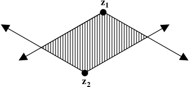
Figure 1. Illustration of two opposite vertices of a hexagon. The hexagon must be contained in the shaded region.

Therefore, the hexagon corresponding to $gI$ is not contained in any of the hexagons corresponding to elements of $Y$. This means that $gI$ is not in the closure of $Y$ in $X_{x}(\epsilon^{\nu})$. Since this was true for any $gI\notin Y$, it follows that $Y$ is closed in $X_{x}(\epsilon^{\nu})$. ∎

Theorem 6.

Assume that $\nu$ is strictly dominant, that $X_{x}(\epsilon^{\nu})\cap U_{1}wI$ is empty for all but one $w\in W$, and that there is a $w_{1}\in W$ and $y_{1},y_{2}\in\widetilde{W}$ such that if $E$ is the hexagon corresponding to any element of $X_{x}(\epsilon^{\nu})\cap U_{1}wI$ the $w_{1}$ corner of $E$ is given by $y_{1}$ and the $\eta w_{1}$ corner of $E$ is given by $y_{2}$. Then the representation of $A(\mathfrak{o}_{F})$ on the Borel-Moore homology of $X_{x}(\epsilon^{\nu})$ which is induced by the left-multiplication action of $A(\mathfrak{o}_{F})$ on $X_{x}(\epsilon^{\nu})$ is trivial. Furthermore, the representation of $A(F)$ on the Borel-Moore homology of $X_{x}(\epsilon^{\nu})$ simply permutes the homology spaces of translates of the one nonempty intersection $X_{x}(\epsilon^{\nu})\cap U_{1}wI$.

Proof.

Let $w_{0}\in W$ be the unique Weyl group element such that $X_{x}(\epsilon^{\nu})\cap U_{1}w_{0}I$ is nonempty. Since $X_{x}(\epsilon^{\nu})$ is the disjoint union of sets of the form $X_{x}(\epsilon^{\nu})\cap U_{1}\widetilde{w}I$ for $\widetilde{w}\in\widetilde{W}$, we see that by Proposition 4.0.1 $X_{x}(\epsilon^{\nu})\cap U_{1}w_{0}I$ is closed. Now by Theorem 4, our conclusion follows. ∎

Now, we will consider all possible $x\in\widetilde{W}$ and $\nu=(i,j,k)$. We will reduce the set of combinations of $x$ and $\nu$ that we need to consider, and show that $\nu$ can always be assumed to be dominant. Then for each remaining combination of $x$ and $\nu$ we will show that either Theorem 5 or Theorem 6 or applies.

4.1. Reduction Steps

Following Beazley [1], we define two outer automorphisms of $SL_{3}(L)$ that preserve $I$ and commute with $\sigma$.

Let

$$\tau:=\begin{pmatrix}0&0&\epsilon^{-1}\\ 1&0&0\\ 0&1&0\end{pmatrix}$$

and define $\varphi(g):=\tau g\tau^{-1}$. Then $\varphi$ is an automorphism of $SL_{3}(L)$ of order 3, clearly commutes with $\sigma$, since $\sigma(\tau)=\tau$, and by explicit computation preserves $I$. Also by explicit computation, if $w\in W$, then

$$\varphi(\epsilon^{(\mu_{1},\mu_{2},\mu_{3})}w)=\epsilon^{(-1,0,0)+s_{1}s_{2}w(0,0,1)+s_{1}s_{2}(\mu_{1},\mu_{2},\mu_{3})}s_{1}s_{2}ws_{2}s_{1}.$$

In particular,

$$\varphi(s_{1})=s_{2}\quad\mbox{and}\quad\varphi(s_{2})=s_{1}s_{2}s_{1}=s_{2}s_{1}s_{2}.$$

Define $\psi(g):=\eta(g^{t})^{-1}\eta^{-1}$, where $\eta$ is the maximal length element of $W$. Then $\psi$ is an automorphism of $SL_{3}(L)$ of order 2, commutes with $\sigma$, since $\sigma(\eta)=\eta$, and by explicit computation preserves $I$. Also by explicit computation, if $w\in W$, then

$$\psi(\epsilon^{(\mu_{1},\mu_{2},\mu_{3})}w)=\epsilon^{-\eta(\mu_{1},\mu_{2},\mu_{3})}\eta w\eta.$$

In particular,

$$\psi(s_{1})=s_{2}\quad\mbox{and}\quad\psi(s_{2})=s_{1}.$$

Since $\varphi$ and $\psi$ preserve $I$ and commute with $\sigma$, we see that

$$X_{x}(\epsilon^{\nu})\cong\varphi(X_{x}(\epsilon^{\nu}))=X_{\varphi(x)}(\epsilon^{s_{1}s_{2}\nu})$$

and

$$X_{x}(\epsilon^{\nu})\cong\psi(X_{x}(\epsilon^{\nu}))=X_{\psi(x)}(\epsilon^{-\eta\nu}).$$

Now let $t\in A(\mathfrak{o}_{F})$. Then

$$\varphi(tg)=\varphi(t)\varphi(g)=t^{\prime}\varphi(g)$$

where $t^{\prime}=s_{1}s_{2}ts_{2}s_{1}\in A(\mathfrak{o}_{F})$. Similarly,

$$\psi(tg)=\psi(t)\psi(g)=t^{\prime}\psi(g)$$

where $t^{\prime}=\eta t^{-1}\eta\in A(\mathfrak{o}_{F})$.

As we can see, $\varphi$ and $\psi$ do not commute with the left-multiplication action of $A(\mathfrak{o}_{F})$ on $X_{x}(\epsilon^{\nu})$, but under these isomorphisms this action becomes the composition of some endomorphism of $A(\mathfrak{o}_{F})$ and the left-multiplication action. As a result, if all elements of $A(\mathfrak{o}_{F})$ act trivially on the homology of $\varphi(X_{x}(\epsilon^{\nu}))$ or $\psi(X_{x}(\epsilon^{\nu}))$, then they all act trivially on the homology of $X_{x}(\epsilon^{\nu})$.

There is also an isomorphism between $X_{x}(\epsilon^{\nu})$ and $X_{x}(\epsilon^{w\nu})$, as discussed in [2], given by left-multiplication by $w$. Again, this isomorphism does not commute with the left-multiplication action of $A(\mathfrak{o}_{F})$, but under this isomorphism this action becomes a composition of the conjugation action of $w$ on $A(\mathfrak{o}_{F})$ and the left-multiplication action. As a result, if all elements of $A(\mathfrak{o}_{F})$ act trivially on the cohomology of $X_{x}(\epsilon^{w\nu})$, then they all act trivially on the cohomology of $X_{x}(\epsilon^{\nu})$. Since by assumption the integers in $\nu$ are all distinct, by appropriate choice of $w$, we can always. without changing $x$, reduce to the case where $\nu$ is strictly dominant: $\nu=(\nu_{1},\nu_{2},\nu_{3})$, with $\nu_{1}>\nu_{2}>\nu_{3}$.

Now we will use $\varphi$, $\psi$, and left-multiplication by appropriate $w$ to reduce the number of cases we need to consider. There are three possibilities, depending on $x$.

• The permutation part of $x$ is the identity. In this case, $x=\epsilon^{(\mu_{1},\mu_{2},\mu_{3})}$, so

  $$\varphi(x)=\epsilon^{(\mu_{3},\mu_{1},\mu_{2})}$$

  and

  $$\varphi^{2}(x)=\epsilon^{(\mu_{2},\mu_{3},\mu_{1})}.$$

  Thus we can use $\varphi$ to reduce to the cases where $\mu_{3}\leq\mu_{2}\leq\mu_{1}$ or $\mu_{1}\leq\mu_{2}\leq\mu_{3}$, then use $\psi$ to reduce to the cases which have $\mu_{3}\leq\mu_{2}\leq\mu_{1}$, and finally use left-multiplication by the appropriate $w$ to make sure $\nu=(i,j,k)$ is strictly dominant. So all cases where the permutation part of $x$ is the identity reduce to the cases where $\nu$ is strictly dominant,

  $$x=\begin{pmatrix}\epsilon^{d}&0&0\\ 0&\epsilon^{e}&0\\ 0&0&\epsilon^{f}\end{pmatrix},$$

  and $f\leq e\leq d$.

• The permutation part of $x$ is a transposition. Since $\varphi(s_{2})=\varphi^{2}(s_{1})=\eta$, we can use $\varphi$ to reduce to the cases where the permutation part of $x$ is $\eta$. Then we can use left-multiplication by the appropriate $w$ to reduce to the cases where $\nu$ is strictly dominant. Now if $\nu=(i,j,k)$ and $x=\epsilon^{(d,e,f)}\eta$, then $\psi(X_{x}(\epsilon^{\nu}))=X_{x^{\prime}}(\epsilon^{\nu^{\prime}})$ where $\nu^{\prime}=(-k,-j,-i)$ and $x^{\prime}=\epsilon^{(-f,-e,-d)}\eta$. In particular, by using $\psi$ we can make sure that either $e$ is maximal in $\{d,e,f\}$ or that it’s not minimal and $e\geq j$. Note that if $\nu$ was strictly dominant, so is $\nu^{\prime}$. So all cases in which the permutation part of $x$ is a transposition reduce to the cases where $\nu=(i,j,k)$ is strictly dominant,

  $$x=\begin{pmatrix}0&0&\epsilon^{d}\\ 0&\epsilon^{e}&0\\ \epsilon^{f}&0&0\end{pmatrix},$$

  and one of the following four conditions holds:

  • $f\leq d<e$

  • $f\leq e\leq d$ and $e\geq j$

  • $d<f\leq e$

  • $d<e<f$ and $e\geq j$.

• The permutation part of $x$ is a 3-cycle. Since $\psi(s_{1}s_{2})=s_{2}s_{1}$, we can use $\psi$ to reduce to the cases where the permutation part of $x$ is $s_{2}s_{1}$. Further, given $x=\epsilon^{(\mu_{1},\mu_{2},\mu_{3})}s_{2}s_{1}$, we have:

  $$\varphi(x)=\epsilon^{(\mu_{3}-1,\mu_{1},\mu_{2}+1)}s_{2}s_{1}$$

  and

  $$\varphi^{2}(x)=\epsilon^{(\mu_{2},\mu_{3}-1,\mu_{1}+1)}s_{2}s_{1}.$$

  Thus one of $x,\varphi(x),\varphi^{2}(x)$ is of the form $\epsilon^{\mu}s_{2}s_{1}$, where $\mu=(\mu_{1},\mu_{2},\mu_{3})$ and $\mu_{3}>\max(\mu_{1},\mu_{2})$. Therefore, we can reduce all cases where the permutation part of $x$ is a 3-cycle to the case

  $$x=\begin{pmatrix}0&\epsilon^{d}&0\\ 0&0&\epsilon^{e}\\ \epsilon^{f}&0&0\end{pmatrix}$$

  where $d<f$ and $e<f$. We will treat this as two cases: $d\leq e<f$, and $e<d<f$. Using left-multiplication by the appropriate $w$ we can further reduce to the cases where $\nu$ is strictly dominant.

Note that in all cases, we have reduced to the situation where $\nu$ is strictly dominant.

4.2. Hexagons Corresponding to Certain Elements of $X$

We will now look at various types of elements of $X$ that can arise in the cases that we will consider. For each such element $gI$, we will compute the possible hexagons that could correspond to it by finding, for each $U^{\prime}$ (a conjugate of $U_{1}$ by an element of $W$) the possible $\widetilde{w}\in\widetilde{W}$ such that $g\in U^{\prime}\widetilde{w}I$, as described in Section 2.2. As described in that section, we will repeatedly look for the leftmost entry in a given row of some matrix which has valuation minimal amongst the entries in that row. We will refer to such an entry as a “minimal entry.”

4.2.1. Hexagons of Elements of $U_{1}I$

Let

$$g=\begin{pmatrix}1&a&b\\ 0&1&c\\ 0&0&1\end{pmatrix}$$

be an element of $U_{1}$, and assume that it satisfies the following conditions:

• If $\mathop{\mathrm{val}}(b)\geq 0$, then $\mathop{\mathrm{val}}(a)<0$.

• If $\mathop{\mathrm{val}}(c)\geq 0$, then $\mathop{\mathrm{val}}(b-ac)<0$.

• If $\mathop{\mathrm{val}}(b)\geq\mathop{\mathrm{val}}(a)$, then $\mathop{\mathrm{val}}(b-ac)<0$.

If $U^{\prime}=U_{1}$, we look at the rows of $g$ in the order 3,2,1. There is only one nonzero entry in the third row. Once we have eliminated the other entries in the third column, the matrix we are left with is

(12) $$\begin{pmatrix}1&a&0\\ 0&1&0\\ 0&0&1\end{pmatrix}.$$

There is only one nonzero entry in the second row, so in this case

$$\widetilde{w}=\begin{pmatrix}1&0&0\\ 0&1&0\\ 0&0&1\end{pmatrix}.$$

If $U^{\prime}=s_{1}U_{1}s_{1}$, we look at the rows of $g$ in the order 3,1,2. After the first step our matrix is the one in (12). Now we look for the minimal entry in the first row of this simplified matrix. Which entry in the first row is minimal depends on $\mathop{\mathrm{val}}(a)$, and we see that

$$\widetilde{w}=\begin{pmatrix}0&\epsilon^{\mathop{\mathrm{val}}(a)}&0\\ \epsilon^{-\mathop{\mathrm{val}}(a)}&0&0\\ 0&0&1\end{pmatrix}$$

if $\mathop{\mathrm{val}}(a)<0$ and

$$\widetilde{w}=\begin{pmatrix}1&0&0\\ 0&1&0\\ 0&0&1\end{pmatrix}.$$

otherwise.

If $U^{\prime}=s_{2}U_{1}s_{2}$, we look at the rows of $g$ in the order 2,3,1. In the second row, the minimal entry depends on $\mathop{\mathrm{val}}(c)$, but in either case there is only one nonzero entry in the third row. We see that

$$\widetilde{w}=\begin{pmatrix}1&0&0\\ 0&0&\epsilon^{\mathop{\mathrm{val}}(c)}\\ 0&\epsilon^{-\mathop{\mathrm{val}}(c)}&0\end{pmatrix}$$

if $\mathop{\mathrm{val}}(c)<0$ and

$$\widetilde{w}=\begin{pmatrix}1&0&0\\ 0&1&0\\ 0&0&1\end{pmatrix}.$$

otherwise.

If $U^{\prime}=s_{2}s_{1}U_{1}s_{1}s_{2}$, we look at the rows of $g$ in the order 2,1,3. If $\mathop{\mathrm{val}}(c)<0$, then the minimal entry in the second row is $c$, and once we have eliminated the other entries in the second row and third column the matrix we are left with is

$$\begin{pmatrix}1&a-\frac{b}{c}&0\\ 0&0&c\\ 0&-\frac{1}{c}&0\end{pmatrix}.$$

The minimal entry in the first row depends on how $\mathop{\mathrm{val}}(b-ac)$ and $\mathop{\mathrm{val}}(c)$ compare. If $\mathop{\mathrm{val}}(b-ac)\geq\mathop{\mathrm{val}}(c)$, then the minimal entry is 1, and

$$\widetilde{w}=\begin{pmatrix}1&0&0\\ 0&0&\epsilon^{\mathop{\mathrm{val}}(c)}\\ 0&\epsilon^{-\mathop{\mathrm{val}}(c)}&0\end{pmatrix}.$$

Otherwise, the minimal entry is $a-b/c$ and

$$\widetilde{w}=\begin{pmatrix}0&\epsilon^{\mathop{\mathrm{val}}(b-ac)-\mathop{\mathrm{val}}(c)}&0\\ 0&0&\epsilon^{\mathop{\mathrm{val}}(c)}\\ \epsilon^{-\mathop{\mathrm{val}}(b-ac)}&0&0\end{pmatrix}.$$

If, on the other hand, $\mathop{\mathrm{val}}(c)\geq 0$, then the minimal entry in the second row is $1$, and once we have eliminated the other entries in the second row and second column the matrix we are left with is

$$\begin{pmatrix}1&0&b-ac\\ 0&1&0\\ 0&0&1\end{pmatrix}.$$

Since in this case, by assumption, $\mathop{\mathrm{val}}(b-ac)<0$, $b-ac$ is the minimal entry in the first row, and we see that

$$\widetilde{w}=\begin{pmatrix}0&0&\epsilon^{\mathop{\mathrm{val}}(b-ac)}\\ 0&1&0\\ \epsilon^{-\mathop{\mathrm{val}}(b-ac)}&0&0\end{pmatrix}.$$

If $U^{\prime}=s_{1}s_{2}U_{1}s_{2}s_{1}$, we look at the rows of $g$ in the order 1,3,2. Since $\mathop{\mathrm{val}}(a)<0$ if $\mathop{\mathrm{val}}(b)\geq 0$, the minimal entry in the first row is either $a$ or $b$. If $\mathop{\mathrm{val}}(b)<\mathop{\mathrm{val}}(a)$, this entry is $b$, and after eliminating the other entries in the first row and third column we are left with

(13) $$\begin{pmatrix}0&0&b\\ -\frac{c}{b}&1-\frac{ac}{b}&0\\ -\frac{1}{b}&-\frac{a}{b}&0\end{pmatrix}.$$

In this case, $\widetilde{w}$ depends on how $\mathop{\mathrm{val}}(a)$ compares to 0. If $\mathop{\mathrm{val}}(a)<0$, we get

$$\widetilde{w}=\begin{pmatrix}0&0&\epsilon^{\mathop{\mathrm{val}}(b)}\\ \epsilon^{-\mathop{\mathrm{val}}(a)}&0&0\\ 0&\epsilon^{\mathop{\mathrm{val}}(a)-\mathop{\mathrm{val}}(b)}&0\end{pmatrix}.$$

Otherwise, we get

$$\widetilde{w}=\begin{pmatrix}0&0&\epsilon^{\mathop{\mathrm{val}}(b)}\\ 0&1&0\\ \epsilon^{-\mathop{\mathrm{val}}(b)}&0&0\end{pmatrix}.$$

If, instead, $\mathop{\mathrm{val}}(b)\geq\mathop{\mathrm{val}}(a)$, then the minimal entry in the first row is $a$, and after eliminating the other entries in the first row and second column we are left with

(14) $$\begin{pmatrix}0&a&0\\ -\frac{1}{a}&0&c-\frac{b}{a}\\ 0&0&1\end{pmatrix}.$$

There is only one nonzero entry in the third row, so we get

$$\widetilde{w}=\begin{pmatrix}0&\epsilon^{\mathop{\mathrm{val}}(a)}&0\\ \epsilon^{-\mathop{\mathrm{val}}(a)}&0&0\\ 0&0&1\end{pmatrix}.$$

If $U^{\prime}=s_{1}s_{2}s_{1}U_{1}s_{1}s_{2}s_{1}$, we look at the rows of $g$ in the order 1,2,3. After the first step, if $\mathop{\mathrm{val}}(b)<\mathop{\mathrm{val}}(a)$, we are left with the matrix in (13). The minimal entry in the second row depends on how $\mathop{\mathrm{val}}(b-ac)$ compares to $\mathop{\mathrm{val}}(c)$. If $\mathop{\mathrm{val}}(b-ac)<\mathop{\mathrm{val}}(c)$, then we get

$$\widetilde{w}=\begin{pmatrix}0&0&\epsilon^{\mathop{\mathrm{val}}(b)}\\ 0&\epsilon^{\mathop{\mathrm{val}}(b-ac)-\mathop{\mathrm{val}}(b)}&0\\ \epsilon^{-\mathop{\mathrm{val}}(b-ac)}&0&0\end{pmatrix}.$$

Otherwise, we get

$$\widetilde{w}=\begin{pmatrix}0&0&\epsilon^{\mathop{\mathrm{val}}(b)}\\ \epsilon^{\mathop{\mathrm{val}}(c)-\mathop{\mathrm{val}}(b)}&0&0\\ 0&\epsilon^{-\mathop{\mathrm{val}}(c)}&0\end{pmatrix}.$$

If, on the other hand, $\mathop{\mathrm{val}}(b)\geq\mathop{\mathrm{val}}(a)$, then we are left with the matrix in (14). Since in this case $\mathop{\mathrm{val}}(b-ac)<0$ by assumption, we get

$$\widetilde{w}=\begin{pmatrix}0&\epsilon^{\mathop{\mathrm{val}}(a)}&0\\ 0&0&\epsilon^{\mathop{\mathrm{val}}(b-ac)-\mathop{\mathrm{val}}(a)}\\ \epsilon^{-\mathop{\mathrm{val}}(b-ac)}&0&0\end{pmatrix}.$$

4.2.2. Hexagons of Elements of $U_{1}s_{1}I$

Let

$$g=\begin{pmatrix}a&1&b\\ 1&0&c\\ 0&0&1\end{pmatrix}$$

be an element of $U_{1}s_{1}$, and assume that it satisfies the following conditions:

• $\mathop{\mathrm{val}}(c)<0$.

• If $\mathop{\mathrm{val}}(a)\leq 0$, then $\mathop{\mathrm{val}}(b)<\mathop{\mathrm{val}}(a)$.

If $U^{\prime}=U_{1}$, we look at the rows of $g$ in the order 3,2,1. There is only one nonzero entry in the third row. Once we have eliminated the other entries in the third column, the matrix we are left with is

(15) $$\begin{pmatrix}a&1&0\\ 1&0&0\\ 0&0&1\end{pmatrix}.$$

There is only one nonzero entry in the second row, so we get

$$\widetilde{w}=\begin{pmatrix}0&1&0\\ 1&0&0\\ 0&0&1\end{pmatrix}.$$

If $U^{\prime}=s_{1}U_{1}s_{1}$, we look at the rows of $g$ in the order 3,1,2. After the first step our matrix is the one in (15). Which entry in the first row is minimal depends on $\mathop{\mathrm{val}}(a)$, and we see that

$$\widetilde{w}=\begin{pmatrix}\epsilon^{\mathop{\mathrm{val}}(a)}&0&0\\ 0&\epsilon^{-\mathop{\mathrm{val}}(a)}&0\\ 0&0&1\end{pmatrix}$$

if $\mathop{\mathrm{val}}(a)\leq 0$ and

$$\widetilde{w}=\begin{pmatrix}0&1&0\\ 1&0&0\\ 0&0&1\end{pmatrix}.$$

otherwise.

If $U^{\prime}=s_{2}U_{1}s_{2}$, we look at the rows of $g$ in the order 2,3,1. Since by assumption $\mathop{\mathrm{val}}(c)<0$, $c$ is the minimal entry in the second row. After eliminating the other entries in the second row and third column, we are left with

(16) $$\begin{pmatrix}a-\frac{b}{c}&1&0\\ 0&0&c\\ -\frac{1}{c}&0&0\end{pmatrix}.$$

There is only one nonzero entry in the third row, so we get

$$\widetilde{w}=\begin{pmatrix}0&1&0\\ 0&0&\epsilon^{\mathop{\mathrm{val}}(c)}\\ \epsilon^{-\mathop{\mathrm{val}}(c)}&0&0\end{pmatrix}.$$

If $U^{\prime}=s_{2}s_{1}U_{1}s_{1}s_{2}$, we look at the rows of $g$ in the order 2,1,3. After the first step our matrix is the one in (16). The minimal entry in the first row depends on how $\mathop{\mathrm{val}}(b-ac)$ compares to $\mathop{\mathrm{val}}(c)$. If $\mathop{\mathrm{val}}(b-ac)\leq\mathop{\mathrm{val}}(c)$, then the minimal entry is the first one, and we get

$$\widetilde{w}=\begin{pmatrix}\epsilon^{\mathop{\mathrm{val}}(b-ac)-\mathop{\mathrm{val}}(c)}&0&0\\ 0&0&\epsilon^{\mathop{\mathrm{val}}(c)}\\ 0&\epsilon^{-\mathop{\mathrm{val}}(b-ac)}&0\end{pmatrix}.$$

Otherwise, the minimal entry is the second one, and we get

$$\widetilde{w}=\begin{pmatrix}0&1&0\\ 0&0&\epsilon^{\mathop{\mathrm{val}}(c)}\\ \epsilon^{-\mathop{\mathrm{val}}(c)}&0&0\end{pmatrix}.$$

If $U^{\prime}=s_{1}s_{2}U_{1}s_{2}s_{1}$, we look at the rows of $g$ in the order 1,3,2. Since by assumption either $\mathop{\mathrm{val}}(a)>0$ or $\mathop{\mathrm{val}}(b)<\mathop{\mathrm{val}}(a)$, the minimal entry is either 1 or $b$. If $\mathop{\mathrm{val}}(b)<0$, we eliminate the other entries in the first row and third column and are left with

(17) $$\begin{pmatrix}0&0&b\\ 1-\frac{ac}{b}&-\frac{c}{b}&0\\ -\frac{a}{b}&-\frac{1}{b}&0\end{pmatrix}.$$

In this case, we see that

$$\widetilde{w}=\begin{pmatrix}0&0&\epsilon^{\mathop{\mathrm{val}}(b)}\\ 0&\epsilon^{-\mathop{\mathrm{val}}(a)}&0\\ \epsilon^{\mathop{\mathrm{val}}(a)-\mathop{\mathrm{val}}(b)}&0&0\end{pmatrix}$$

if $\mathop{\mathrm{val}}(a)\leq 0$ and

$$\widetilde{w}=\begin{pmatrix}0&0&\epsilon^{\mathop{\mathrm{val}}(b)}\\ 1&0&0\\ 0&\epsilon^{-\mathop{\mathrm{val}}(b)}&0\end{pmatrix}$$

if $\mathop{\mathrm{val}}(a)>0$. If, on the other hand, $\mathop{\mathrm{val}}(b)\geq 0$, then 1 is the minimal entry in the first row, and after eliminating the other entries in that row and the second column we are left with

(18) $$\begin{pmatrix}0&1&0\\ 1&0&c\\ 0&0&1\end{pmatrix}.$$

Since there is only one nonzero entry in the third row, we get

$$\widetilde{w}=\begin{pmatrix}0&1&0\\ 1&0&0\\ 0&0&1\end{pmatrix}.$$

If $U^{\prime}=s_{1}s_{2}s_{1}U_{1}s_{1}s_{2}s_{1}$, we look at the rows of $g$ in the order 1,2,3. After the first step, if $\mathop{\mathrm{val}}(b)<0$ we are left with the matrix in (17). The minimal entry in the second row depends on how $\mathop{\mathrm{val}}(b-ac)$ compares to $\mathop{\mathrm{val}}(c)$. We get

$$\widetilde{w}=\begin{pmatrix}0&0&\epsilon^{\mathop{\mathrm{val}}(b)}\\ \epsilon^{\mathop{\mathrm{val}}(b-ac)-\mathop{\mathrm{val}}(b)}&0&0\\ 0&\epsilon^{-\mathop{\mathrm{val}}(b-ac)}&0\end{pmatrix}$$

if $\mathop{\mathrm{val}}(b-ac)\leq\mathop{\mathrm{val}}(c)$ and

$$\widetilde{w}=\begin{pmatrix}0&0&\epsilon^{\mathop{\mathrm{val}}(b)}\\ 0&\epsilon^{\mathop{\mathrm{val}}(c)-\mathop{\mathrm{val}}(b)}&0\\ \epsilon^{-\mathop{\mathrm{val}}(c)}&0&0\end{pmatrix}$$

if $\mathop{\mathrm{val}}(b-ac)>\mathop{\mathrm{val}}(c)$. If, on the other hand, $\mathop{\mathrm{val}}(b)\geq 0$, we are left with the matrix in (18). Since $\mathop{\mathrm{val}}(c)<0$ by assumption, in this case we get

$$\widetilde{w}=\begin{pmatrix}0&1&0\\ 0&0&\epsilon^{\mathop{\mathrm{val}}(c)}\\ \epsilon^{-\mathop{\mathrm{val}}(c)}&0&0\end{pmatrix}.$$

4.2.3. Hexagons of Elements of $U_{1}s_{2}I$

Let

$$g=\begin{pmatrix}1&b&a\\ 0&c&1\\ 0&1&0\end{pmatrix}$$

be an element of $U_{1}s_{2}$, and assume that it satisfies the following conditions:

• $\mathop{\mathrm{val}}(a)<0$.

• $\mathop{\mathrm{val}}(b-ac)<\mathop{\mathrm{val}}(c)$.

• $\mathop{\mathrm{val}}(b-ac)<0$.

If $U^{\prime}=U_{1}$, we look at the rows of $g$ in the order 3,2,1. There is only one nonzero entry in the third row. Once we have eliminated the other entries in the second column, the matrix we are left with is

(19) $$\begin{pmatrix}1&0&a\\ 0&0&1\\ 0&1&0\end{pmatrix}.$$

There is only one nonzero entry in the second row, so we get

$$\widetilde{w}=\begin{pmatrix}1&0&0\\ 0&0&1\\ 0&1&0\end{pmatrix}.$$

If $U^{\prime}=s_{1}U_{1}s_{1}$, we look at the rows of $g$ in the order 3,1,2. After the first step our matrix is the one in (19). Since $\mathop{\mathrm{val}}(a)<0$, the lowest-valuation entry in the first row is $a$, and we get

$$\widetilde{w}=\begin{pmatrix}0&0&\epsilon^{\mathop{\mathrm{val}}(a)}\\ \epsilon^{-\mathop{\mathrm{val}}(a)}&0&0\\ 0&1&0\end{pmatrix}.$$

If $U^{\prime}=s_{2}Us_{2}$, we look at the rows of $g$ in the order 2,3,1. In the second row the minimal entry depends on the valuation of $c$. If $\mathop{\mathrm{val}}(c)\leq 0$, then the minimal entry is $c$. Once we have eliminated the other entries in the second row and second column, the matrix we are left with is

(20) $$\begin{pmatrix}1&0&a-\frac{b}{c}\\ 0&c&0\\ 0&0&-\frac{1}{c}\end{pmatrix}.$$

If $\mathop{\mathrm{val}}(c)>0$, then the minimal entry in the second row is 1. Once we have eliminated the entries in the second row and third column, the matrix we are left with is

(21) $$\begin{pmatrix}1&b-ac&0\\ 0&0&1\\ 0&1&0\end{pmatrix}.$$

In either case, there is only one nonzero entry in the third row so we get

$$\widetilde{w}=\begin{pmatrix}1&0&0\\ 0&\epsilon^{\mathop{\mathrm{val}}(c)}&0\\ 0&0&\epsilon^{-\mathop{\mathrm{val}}(c)}\end{pmatrix}$$

if $\mathop{\mathrm{val}}(c)\leq 0$ and

$$\widetilde{w}=\begin{pmatrix}1&0&0\\ 0&0&1\\ 0&1&0\end{pmatrix}$$

if $\mathop{\mathrm{val}}(c)>0$.

If $U^{\prime}=s_{2}s_{1}Us_{1}s_{2}$, we look at the rows of $g$ in the order 2,1,3. As for $U^{\prime}=s_{2}Us_{2}$, after the first step we are left with either the matrix in (20) or the matrix in (21), depending on $\mathop{\mathrm{val}}(c)$. If $\mathop{\mathrm{val}}(c)\leq 0$, then because $\mathop{\mathrm{val}}(b-ac)<\mathop{\mathrm{val}}(c)$ the minimal entry in the first row is $a-b/c$. So in this case

$$\widetilde{w}=\begin{pmatrix}0&0&\epsilon^{\mathop{\mathrm{val}}(b-ac)-\mathop{\mathrm{val}}(c)}\\ 0&\epsilon^{\mathop{\mathrm{val}}(c)}&0\\ \epsilon^{-\mathop{\mathrm{val}}(b-ac)}&0&0\end{pmatrix}.$$

If $\mathop{\mathrm{val}}(c)>0$, then, because $\mathop{\mathrm{val}}(b-ac)<0$, the minimal entry in the first row is $b-ac$. So in this case

$$\widetilde{w}=\begin{pmatrix}0&e^{\mathop{\mathrm{val}}(b-ac)}&0\\ 0&0&1\\ e^{-\mathop{\mathrm{val}}(b-ac)}&0&0\end{pmatrix}.$$

If $U^{\prime}=s_{1}s_{2}Us_{2}s_{1}$, we look at the rows of $g$ in the order 1,3,2. Since $\mathop{\mathrm{val}}(a)<0$, the minimal entry must be $a$ or $b$. If it is $a$, then once we have eliminated the other entries in the first row and third column the matrix we are left with is

(22) $$\begin{pmatrix}0&0&a\\ -\frac{1}{a}&c-\frac{b}{a}&0\\ 0&1&0\end{pmatrix}.$$

There is only one nonzero entry in the third row, so in this case

$$\widetilde{w}=\begin{pmatrix}0&0&\epsilon^{\mathop{\mathrm{val}}(a)}\\ \epsilon^{-\mathop{\mathrm{val}}(a)}&0&0\\ 0&1&0\end{pmatrix}.$$

If the minimal entry in the first row is $b$, then once we have eliminated the other entries in the first row and second column, the matrix we are left with is

(23) $$\begin{pmatrix}0&b&0\\ -\frac{c}{b}&0&1-\frac{ac}{b}\\ -\frac{1}{b}&0&-\frac{a}{b}\end{pmatrix}.$$

Since $\mathop{\mathrm{val}}(a)<0$, the minimal entry in the third row is $-a/b$, so in this case

$$\widetilde{w}=\begin{pmatrix}0&\epsilon^{\mathop{\mathrm{val}}(b)}&0\\ \epsilon^{-\mathop{\mathrm{val}}(a)}&0&0\\ 0&0&\epsilon^{\mathop{\mathrm{val}}(a)-\mathop{\mathrm{val}}(b)}\end{pmatrix}.$$

If $U^{\prime}=s_{1}s_{2}s_{1}Us_{1}s_{2}s_{1}$, we look at the rows of $g$ in the order 1,2,3. After the first step we are left with the matrix in (22) if $\mathop{\mathrm{val}}(a)<\mathop{\mathrm{val}}(b)$ or the matrix in (23) if $\mathop{\mathrm{val}}(a)\geq\mathop{\mathrm{val}}(b)$. In the former case, since $\mathop{\mathrm{val}}(b-ac)<0$, we have

$$\widetilde{w}=\begin{pmatrix}0&0&\epsilon^{\mathop{\mathrm{val}}(a)}\\ 0&\epsilon^{\mathop{\mathrm{val}}(b-ac)-\mathop{\mathrm{val}}(a)}&0\\ \epsilon^{-\mathop{\mathrm{val}}(b-ac)}&0&0\end{pmatrix}.$$

In the latter case, since $\mathop{\mathrm{val}}(b-ac)<c$, we have

$$\widetilde{w}=\begin{pmatrix}0&\epsilon^{\mathop{\mathrm{val}}(b)}&0\\ 0&0&\epsilon^{\mathop{\mathrm{val}}(b-ac)-\mathop{\mathrm{val}}(b)}\\ \epsilon^{-\mathop{\mathrm{val}}(b-ac)}&0&0\end{pmatrix}.$$

4.2.4. Hexagons of Elements of $U_{1}s_{2}s_{1}I$

Let

$$g=\begin{pmatrix}b&1&a\\ c&0&1\\ 1&0&0\end{pmatrix}$$

be an element of $U_{1}s_{2}s_{1}$, and assume that it satisfies the following conditions:

• $\mathop{\mathrm{val}}(c)\leq 0$.

• $\mathop{\mathrm{val}}(a)\geq 0$.

• $\mathop{\mathrm{val}}(b)\geq\mathop{\mathrm{val}}(c)$.

Since $\mathop{\mathrm{val}}(a)\geq 0$, it can be eliminated by the right-action of $I$ without changing anything else in $g$, so we can assume that $a=0$.

If $U^{\prime}=U_{1}$, we look at the rows of $g$ in the order 3,2,1. If $U^{\prime}=s_{1}U_{1}s_{1}$, we look at the rows of $g$ in the order 3,1,2. In either case, there is only one nonzero entry in the third row, and once we have eliminated the other entries in the first column we are left with

$$\widetilde{w}=\begin{pmatrix}0&1&0\\ 0&0&1\\ 1&0&0\end{pmatrix}.$$

If $U^{\prime}=s_{2}U_{1}s_{2}$, we look at the rows of $g$ in the order 2,3,1. If $U^{\prime}=s_{2}s_{1}U_{1}s_{1}s_{2}$, we look at the rows of $g$ in the order 2,1,3. In either case, by assumption $\mathop{\mathrm{val}}(c)\leq 0$, so $c$ is the minimal entry in the second row. After eliminating the other entries in the second row and first column, we are left with

(24) $$\begin{pmatrix}0&1&-\frac{b}{c}\\ c&0&0\\ 0&0&-\frac{1}{c}\end{pmatrix}.$$

Since by assumption $\mathop{\mathrm{val}}(b)\geq\mathop{\mathrm{val}}(c)$, the $-b/c$ entry can be eliminated by the right-action of $I$ without changing anything else in $g$. So we see that in both of these cases

$$\widetilde{w}=\begin{pmatrix}0&1&0\\ \epsilon^{\mathop{\mathrm{val}}(c)}&0&0\\ 0&0&\epsilon^{-\mathop{\mathrm{val}}(c)}\end{pmatrix}.$$

If $U^{\prime}=s_{1}s_{2}U_{1}s_{2}s_{1}$, we look at the rows of $g$ in the order 1,3,2. The minimal entry in the first row depends on the valuation of $b$. If $\mathop{\mathrm{val}}(b)\leq 0$, then $b$ is the minimal entry, and after eliminating the other entries in the first row and first column we are left with

(25) $$\begin{pmatrix}b&0&0\\ 0&-\frac{c}{b}&1\\ 0&-\frac{1}{b}&0\end{pmatrix}.$$

There is only one nonzero entry in the third row, so in this case

$$\widetilde{w}=\begin{pmatrix}\epsilon^{\mathop{\mathrm{val}}(b)}&0&0\\ 0&0&1\\ 0&\epsilon^{-\mathop{\mathrm{val}}(b)}&0\end{pmatrix}.$$

If, on the other hand, $\mathop{\mathrm{val}}(b)>0$, then the minimal entry in the first row is $1$, and after eliminating the $b$ we are left with

(26) $$\begin{pmatrix}0&1&0\\ c&0&1\\ 1&0&0\end{pmatrix}.$$

There is only one nonzero entry in the third row, so

$$\widetilde{w}=\begin{pmatrix}0&1&0\\ 0&0&1\\ 1&0&0\end{pmatrix}.$$

If $U^{\prime}=s_{1}s_{2}s_{1}U_{1}s_{1}s_{2}s_{1}$, we look at the rows of $g$ in the order 1,2,3. After the first step, if $\mathop{\mathrm{val}}(b)\leq 0$ we are left with the matrix in (25). Since $\mathop{\mathrm{val}}(c)\leq\mathop{\mathrm{val}}(b)$, the minimal entry in the second row is $-c/b$, and we get

$$\widetilde{w}=\begin{pmatrix}\epsilon^{\mathop{\mathrm{val}}(b)}&0&0\\ 0&\epsilon^{\mathop{\mathrm{val}}(c)-\mathop{\mathrm{val}}(b)}&0\\ 0&0&\epsilon^{-\mathop{\mathrm{val}}(c)}\end{pmatrix}.$$

If, on the other hand, $\mathop{\mathrm{val}}(b)>0$, we are left with the matrix in (26). Since $\mathop{\mathrm{val}}(c)\leq 0$ by assumption, the minimal entry in the second row is $c$ and we get

$$\begin{pmatrix}0&1&0\\ \epsilon^{\mathop{\mathrm{val}}(c)}&0&0\\ 0&0&\epsilon^{-\mathop{\mathrm{val}}(c)}\end{pmatrix}.$$

4.2.5. Hexagons of Elements of $U_{1}s_{1}s_{2}s_{1}I$

Let

$$g=\begin{pmatrix}b&a&1\\ c&1&0\\ 1&0&0\end{pmatrix}$$

be an element of $U_{1}s_{1}s_{2}s_{1}$, and assume that it satisfies the following conditions:

• If $\mathop{\mathrm{val}}(b)>0$, then $\mathop{\mathrm{val}}(a)\leq 0$.

• $\mathop{\mathrm{val}}(b-ac)\leq\mathop{\mathrm{val}}(c)$.

• $\mathop{\mathrm{val}}(b-ac)\leq 0$.

If $U^{\prime}=U_{1}$, we look at the rows of $g$ in the order 3,2,1. There is only one nonzero entry in the third row. Once we have eliminated the other entries in the first column, the matrix we are left with is

(27) $$\begin{pmatrix}0&a&1\\ 0&1&0\\ 1&0&0\end{pmatrix}.$$

There is only one nonzero entry in the second row, so in this case

$$\widetilde{w}=\begin{pmatrix}0&0&1\\ 0&1&0\\ 1&0&0\end{pmatrix}.$$

If $U^{\prime}=s_{1}U_{1}s_{1}$, we look at the rows of $g$ in the order 3,1,2. After the first step our matrix is the one in (27). Which entry in the first row is minimal depends on $\mathop{\mathrm{val}}(a)$, and we see that

$$\widetilde{w}=\begin{pmatrix}0&\epsilon^{\mathop{\mathrm{val}}(a)}&0\\ 0&0&\epsilon^{-\mathop{\mathrm{val}}(a)}\\ 1&0&0\end{pmatrix}$$

if $\mathop{\mathrm{val}}(a)\leq 0$ and

$$\widetilde{w}=\begin{pmatrix}0&0&1\\ 0&1&0\\ 1&0&0\end{pmatrix}.$$

otherwise.

If $U^{\prime}=s_{2}U_{1}s_{2}$, we look at the rows of $g$ in the order 2,3,1. In the second row, the minimal entry depends on $\mathop{\mathrm{val}}(c)$, but in either case there is only one nonzero entry in the third row. We see that

$$\widetilde{w}=\begin{pmatrix}0&0&1\\ \epsilon^{\mathop{\mathrm{val}}(c)}&0&0\\ 0&\epsilon^{-\mathop{\mathrm{val}}(c)}&0\end{pmatrix}$$

if $\mathop{\mathrm{val}}(c)\leq 0$ and

$$\widetilde{w}=\begin{pmatrix}0&0&1\\ 0&1&0\\ 1&0&0\end{pmatrix}.$$

otherwise.

If $U^{\prime}=s_{2}s_{1}U_{1}s_{1}s_{2}$, we look at the rows of $g$ in the order 2,1,3. If $\mathop{\mathrm{val}}(c)\leq 0$, then the minimal entry in the second row is $c$, and once we have eliminated the other entries in the second row and third column the matrix we are left with is

$$\begin{pmatrix}0&a-\frac{b}{c}&1\\ c&0&0\\ 0&-\frac{1}{c}&0\end{pmatrix}.$$

Since $\mathop{\mathrm{val}}(b-ac)\leq\mathop{\mathrm{val}}(c)$, the minimal entry in the first row is $a-b/c$, and

$$\widetilde{w}=\begin{pmatrix}0&\epsilon^{\mathop{\mathrm{val}}(b-ac)-\mathop{\mathrm{val}}(c)}&0\\ \epsilon^{\mathop{\mathrm{val}}(c)}&0&0\\ 0&0&\epsilon^{-\mathop{\mathrm{val}}(b-ac)}\end{pmatrix}.$$

If, on the other hand, $\mathop{\mathrm{val}}(c)>0$, then the minimal entry in the second row is $1$, and once we have eliminated the other entries in the second row and second column the matrix we are left with is

$$\begin{pmatrix}b-ac&0&1\\ 0&1&0\\ 1&0&0\end{pmatrix}.$$

Since in this case, by assumption, $\mathop{\mathrm{val}}(b-ac)\leq 0$, $b-ac$ is the minimal entry in the first row, and we see that

$$\widetilde{w}=\begin{pmatrix}\epsilon^{\mathop{\mathrm{val}}(b-ac)}&0&0\\ 0&1&0\\ 0&0&\epsilon^{-\mathop{\mathrm{val}}(b-ac)}\end{pmatrix}.$$

If $U^{\prime}=s_{1}s_{2}U_{1}s_{2}s_{1}$, we look at the rows of $g$ in the order 1,3,2. Since $\mathop{\mathrm{val}}(a)\leq 0$ if $\mathop{\mathrm{val}}(b)>0$, the minimal entry in the first row is either $a$ or $b$. If $\mathop{\mathrm{val}}(b)\leq\mathop{\mathrm{val}}(a)$, this entry is $b$, and after eliminating the other entries in the first row and third column we are left with

(28) $$\begin{pmatrix}b&0&0\\ 0&1-\frac{ac}{b}&-\frac{c}{b}\\ 0&-\frac{a}{b}&-\frac{1}{b}\end{pmatrix}.$$

In this case, $\widetilde{w}$ depends on how $\mathop{\mathrm{val}}(a)$ compares to 0. If $\mathop{\mathrm{val}}(a)\leq 0$, we get

$$\widetilde{w}=\begin{pmatrix}\epsilon^{\mathop{\mathrm{val}}(b)}&0&0\\ 0&0&\epsilon^{-\mathop{\mathrm{val}}(a)}\\ 0&\epsilon^{\mathop{\mathrm{val}}(a)-\mathop{\mathrm{val}}(b)}&0\end{pmatrix}.$$

Otherwise, we get

$$\widetilde{w}=\begin{pmatrix}\epsilon^{\mathop{\mathrm{val}}(b)}&0&0\\ 0&1&0\\ 0&0&\epsilon^{-\mathop{\mathrm{val}}(b)}\end{pmatrix}.$$

If, instead, $\mathop{\mathrm{val}}(b)>\mathop{\mathrm{val}}(a)$, then the minimal entry in the first row is $a$, and after eliminating the other entries in the first row and second column we are left with

(29) $$\begin{pmatrix}0&a&0\\ c-\frac{b}{a}&0&-\frac{1}{a}\\ 1&0&0\end{pmatrix}.$$

There is only one nonzero entry in the third row, so we get

$$\widetilde{w}=\begin{pmatrix}0&\epsilon^{\mathop{\mathrm{val}}(a)}&0\\ 0&0&\epsilon^{-\mathop{\mathrm{val}}(a)}\\ 1&0&0\end{pmatrix}.$$

If $U^{\prime}=s_{1}s_{2}s_{1}U_{1}s_{1}s_{2}s_{1}$, we look at the rows of $g$ in the order 1,2,3. After the first step, if $\mathop{\mathrm{val}}(b)\leq\mathop{\mathrm{val}}(a)$, we are left with the matrix in (28). Since $\mathop{\mathrm{val}}(b-ac)\leq\mathop{\mathrm{val}}(c)$, we get

$$\widetilde{w}=\begin{pmatrix}\epsilon^{\mathop{\mathrm{val}}(b)}&0&\\ 0&\epsilon^{\mathop{\mathrm{val}}(b-ac)-\mathop{\mathrm{val}}(b)}&0\\ 0&0&\epsilon^{-\mathop{\mathrm{val}}(b-ac)}\end{pmatrix}.$$

If, on the other hand, $\mathop{\mathrm{val}}(b)>\mathop{\mathrm{val}}(a)$, then we are left with the matrix in (29). Since in this case $\mathop{\mathrm{val}}(b-ac)\leq 0$ by assumption, we get

$$\widetilde{w}=\begin{pmatrix}0&\epsilon^{\mathop{\mathrm{val}}(a)}&0\\ \epsilon^{\mathop{\mathrm{val}}(b-ac)-\mathop{\mathrm{val}}(a)}&0&0\\ 0&0&\epsilon^{-\mathop{\mathrm{val}}(b-ac)}\end{pmatrix}.$$

4.3. Stratifications of $X_{x}(\epsilon^{\nu})$

For each of our possible values of $x$ and $\nu$, we will examine the intersections $X_{x}(\epsilon^{\nu})\cap U_{1}wI$ for various $w\in W$. We will determine the possible hexagons that correspond to points of the intersection and use those to show that either Theorem 5 or Theorem 6 applies to $X_{x}(\epsilon^{\nu})$.

For every point in $X_{x}(\epsilon^{\nu})\cap U_{1}wI$, we can pick a representative $g\in U_{1}w$. Let

$$g=\begin{pmatrix}1&a&b\\ 0&1&c\\ 0&0&1\end{pmatrix}w$$

for some $a,b,c\in L$. Then

(30) $$h=g^{-1}\epsilon^{\nu}\sigma(g)=w^{-1}\begin{pmatrix}\epsilon^{i}&\alpha&\beta\\ 0&\epsilon^{j}&\gamma\\ 0&0&\epsilon^{k}\end{pmatrix}w$$

where

(31) $$\alpha =\epsilon^{i}\sigma(a)-\epsilon^{j}a$$

(32) $$\beta =\epsilon^{i}\sigma(b)-\epsilon^{k}b-a(\epsilon^{j}\sigma(c)-\epsilon^{k}c)$$

(33) $$=\epsilon^{i}\sigma(b)-\epsilon^{k}b-a\gamma$$

(34) $$\gamma =\epsilon^{j}\sigma(c)-\epsilon^{k}c.$$

(35) $$\beta\epsilon^{j}-\alpha\gamma =\epsilon^{i+j}\sigma(b)-\epsilon^{k+j}b-\epsilon^{i}\sigma(a)\gamma$$

We will now look at each of the cases that we did not eliminate in Section 4.1.

4.3.1. $x=\epsilon^{(d,e,f)}s_{2}s_{1}$, with $d\leq e<f$

Let

(36) $$x=\epsilon^{(d,e,f)}s_{1}s_{2}s_{1}=\begin{pmatrix}0&\epsilon^{d}&0\\ 0&0&\epsilon^{e}\\ \epsilon^{f}&0&0\end{pmatrix}$$

where $d\leq e<f$, with $d+e+f=0$. Let $\nu=(i,j,k)$ with $i>j>k$ and $i+j+k=0$. We will show that the intersection $X_{x}(\epsilon^{\nu})\cap U_{1}wI$ is nonempty for only one value of $w\in W$, and that Theorem 6 applies.

Since $d\leq e<f$, by Theorem 1 the entry in the first row and second column of $h$ must have valuation $d$ and the determinant of the $2\times 2$ minor in the top right-hand corner must have valuation $d+e$. That means that $w$ can only be one of $1$ and $s_{2}$, since for all other values of $w$ either that entry or the determinant of that minor is 0.

If $w=1$, then

$$h=\begin{pmatrix}\epsilon^{i}&\alpha&\beta\\ 0&\epsilon^{j}&\gamma\\ 0&0&\epsilon^{k}\end{pmatrix}.$$

Thus $\mathop{\mathrm{val}}(\alpha)=d$. The valuation of the determinant of the

$$\begin{pmatrix}\alpha&\beta\\ 0&\epsilon^{k}\end{pmatrix}$$

minor must be greater than $d+e$, so

$$\mathop{\mathrm{val}}(\alpha\epsilon^{k}) >d+e$$

$$d+k >d+e$$

$$k >e.$$

If $w=s_{2}$, then

$$h=\begin{pmatrix}\epsilon^{i}&\beta&\alpha\\ 0&\epsilon^{k}&0\\ 0&\gamma&\epsilon^{j}\end{pmatrix}$$

The valuation of the determinant of the minor in the top right-hand corner must be $d+e$. This gives us

$$\mathop{\mathrm{val}}(\alpha\epsilon^{k}) =d+e$$

$$d+k \leq d+e$$

$$k \leq e$$

Therefore, once $k$ and $e$ are fixed there is only one possible value of $w$ for which $X_{x}(\epsilon^{\nu})\cap U_{1}wI$ might be nonempty. If $k>e$ the intersection is only nonempty if $w=1$, and if $k\leq e$ the intersection is only nonempty if $w=s_{2}$.

We now look at these two possibilities.

The case $k>e$.

In this case, $X_{x}(\epsilon^{\nu})\cap U_{1}wI$ is nonempty only if $w=1$, so

$$h=\begin{pmatrix}\epsilon^{i}&\alpha&\beta\\ 0&\epsilon^{j}&\gamma\\ 0&0&\epsilon^{k}\end{pmatrix}.$$

By Theorem 1, the necessary conditions for $h$ to be in $IxI$ include

(37) $$\mathop{\mathrm{val}}(\alpha) =d$$

(38) $$\mathop{\mathrm{val}}(\beta) \geq d$$

(39) $$\mathop{\mathrm{val}}(\alpha\gamma-\beta\epsilon^{j}) =d+e.$$

We will use these to determine the valuations of $a$, $b$, $c$, and $b-ac$.

From (31) and (37) and because $j>k>e\geq d$ by assumption we know that

(40) $$\mathop{\mathrm{val}}(a)=d-j<0.$$

From (38) and our assumption that $k>e$ we know that $\mathop{\mathrm{val}}(\beta\epsilon^{j})\geq d+j>d+k>d+e$. Then (34), (39) and (37) tell us that

$$\mathop{\mathrm{val}}(\alpha\gamma) =d+e$$

$$d+\mathop{\mathrm{val}}(\gamma) =d+e$$

$$\mathop{\mathrm{val}}(\gamma) =e$$

(41) $$\mathop{\mathrm{val}}(c) =e-k<0$$

Using (40) and (41) we see that

(42) $$\mathop{\mathrm{val}}(\epsilon^{j}a\sigma(c))=d+(e-k)<d$$

and

$$\mathop{\mathrm{val}}(\epsilon^{k}ac)=d+e-j<d+(e-k)=\mathop{\mathrm{val}}(\epsilon^{j}a\sigma(c)).$$

By (38), and (32), this means that

$$\mathop{\mathrm{val}}(\epsilon^{i}\sigma(b)-e^{k}b) =d+e-j$$

$$\mathop{\mathrm{val}}(\epsilon^{k}b) =d+e-j$$

(43) $$\mathop{\mathrm{val}}(b) =(d-j)+(e-k)=i-f.$$

Comparing (43) to (40) we see that

(44) $$\mathop{\mathrm{val}}(b)<\mathop{\mathrm{val}}(a),$$

since $e<k$.

Now from (43) we see that

$$\mathop{\mathrm{val}}(\epsilon^{i}\sigma(b))=d+(e-k)+(i-j)>d+(e-k).$$

Since $\mathop{\mathrm{val}}(\beta)\geq d$, by (42) we must have

$$\mathop{\mathrm{val}}(\epsilon^{k}(b-ac)) =d+(e-k)$$

(45) $$\mathop{\mathrm{val}}(b-ac) =d+e-2k=(d-k)+(e-k)<\mathop{\mathrm{val}}(c),$$

where the last inequality follows because $d-k\leq e-k<0$.

Now $\mathop{\mathrm{val}}(a)<0$ and $\mathop{\mathrm{val}}(b-ac)<0$. So the conditions of Section 4.2.1 are satisfied. Since $\mathop{\mathrm{val}}(c)<0$ and $\mathop{\mathrm{val}}(b-ac)<\mathop{\mathrm{val}}(c)$, the hexagon for $g$ has the vertices

$$\begin{array}[]{ccc}&\begin{pmatrix}1&0&0\\ 0&1&0\\ 0&0&1\end{pmatrix}&\\[-10.00002pt] \begin{pmatrix}1&0&0\\ 0&0&\epsilon^{e-k}\\ 0&\epsilon^{k-e}&0\end{pmatrix}&&\begin{pmatrix}0&\epsilon^{d-j}&0\\ \epsilon^{j-d}&0&0\\ 0&0&1\end{pmatrix}\\[20.00003pt] \begin{pmatrix}0&\epsilon^{d-k}&0\\ 0&0&\epsilon^{e-k}\\ \epsilon^{2k+f}&0&0\end{pmatrix}&&\begin{pmatrix}0&0&\epsilon^{i-f}\\ \epsilon^{j-d}&0&0\\ 0&\epsilon^{k-e}&0\end{pmatrix}\\[-10.00002pt] &\begin{pmatrix}0&0&\epsilon^{i-f}\\ 0&\epsilon^{j-k}&0\\ \epsilon^{2k+f}&0&0\end{pmatrix}&\end{array}.$$

This hexagon is completely determined by our choice of $i,j,k,d,e,f$. So all elements of $X_{x}(\epsilon^{\nu})\cap U_{1}I$ have the same corresponding hexagon, and Theorem 6 applies.

The case $k\leq e$. In this case, $X_{x}(\epsilon^{\nu})\cap U_{1}wI$ is nonempty only if $w=s_{2}$, so

$$h=\begin{pmatrix}\epsilon^{i}&\beta&\alpha\\ 0&\epsilon^{k}&0\\ 0&\gamma&\epsilon^{j}\end{pmatrix}.$$

By Theorem 1, necessary conditions for $h$ to be in $IxI$ include

(46) $$\mathop{\mathrm{val}}(\beta) =d$$

(47) $$\mathop{\mathrm{val}}(\epsilon^{k}) >d\implies k>d$$

(48) $$\mathop{\mathrm{val}}(\epsilon^{j+k}) >d+e\implies j+k>d+e\implies i<f$$

(49) $$\mathop{\mathrm{val}}(\alpha\epsilon^{k}) =d+e$$

(50) $$\mathop{\mathrm{val}}(\alpha\gamma-\beta\epsilon^{j}) >d+e.$$

We will use these to determine the valuations of $a$, $b$, $c$, and $b-ac$.

From (31), (49), and (48), we know that

(51) $$\mathop{\mathrm{val}}(a)=d+e-j-k=i-f<0.$$

Lemma 4.3.1.

$\mathop{\mathrm{val}}(c)\leq 0$ if and only if $e\geq j$, and when this happens $\mathop{\mathrm{val}}(c)=j-e$.

Proof.

By (50), $\mathop{\mathrm{val}}(\alpha\gamma)\leq d+e$ if and only if $\mathop{\mathrm{val}}(\beta\epsilon^{j})\leq d+e$. By (46),

$$\mathop{\mathrm{val}}(\beta\epsilon^{j})=d+j.$$

By (49) and (34),

(52) $$\mathop{\mathrm{val}}(\alpha\gamma)=\mathop{\mathrm{val}}(c)+k+d+e-k=\mathop{\mathrm{val}}(c)+d+e.$$

Now we see that

$$j\leq e \iff d+j\leq d+e$$

$$\iff\mathop{\mathrm{val}}(c)+d+e\leq d+e$$

$$\iff\mathop{\mathrm{val}}(c)\leq 0.$$

If $j\leq e$, then, by (50),

$$\mathop{\mathrm{val}}(\alpha\gamma)=\mathop{\mathrm{val}}(\beta\epsilon^{j})=d+j,$$

and then, by (52), $\mathop{\mathrm{val}}(c)=j-e$. ∎

Lemma 4.3.2.

$\mathop{\mathrm{val}}(b)\leq\mathop{\mathrm{val}}(a)$ if and only if $e\geq i$ and when this happens $\mathop{\mathrm{val}}(b)=d+2i$.

Proof.

From (50) and (35) we see that

(53) $$\mathop{\mathrm{val}}(\epsilon^{i+j}\sigma(b)-\epsilon^{j+k}b-\epsilon^{i}\sigma(a)\gamma)>d+e.$$

Now we consider the three possible ways that $e$ can relate to $i$ and $j$.

If $e\geq i$, then $i>j$ implies $e>j$. In this case, by Lemma 4.3.1, (34), and (51),

$$\mathop{\mathrm{val}}(\epsilon^{i}\sigma(a)\gamma) =i+(d+e-j-k)+(j-e+k)$$

(54) $$=d+i$$

Since $e\geq i$, $d+i\leq d+e$. But then (53) tells us that

$$\mathop{\mathrm{val}}(\epsilon^{i+j}\sigma(b)-\epsilon^{j+k}b)=d+i.$$

Therefore

$$\mathop{\mathrm{val}}(b) =d+i-j-k$$

$$=\mathop{\mathrm{val}}(a)+(i-e)$$

$$\leq\mathop{\mathrm{val}}(a)$$

since $i\leq e$. Since $-j-k=i$, in this case $\mathop{\mathrm{val}}(b)=d+2i$.

If $j\leq e<i$, then (4.3.1) still holds, but now $d+i>d+e$. By (53),

$$\mathop{\mathrm{val}}(\epsilon^{i+j}\sigma(b)-\epsilon^{j+k}b)>d+e$$

so $\mathop{\mathrm{val}}(b)>d+e-j-k=\mathop{\mathrm{val}}(a)$.

If $e<j$, then, by Lemma 4.3.1, $\mathop{\mathrm{val}}(c)>0$. This means that by (34) and (51)

$$\mathop{\mathrm{val}}(\epsilon^{i}\sigma(a)\gamma) >i+d+e-j-k+k$$

$$=d+e+(i-j)$$

$$>d+e.$$

So by the same argument as in the case when $j\leq e<i$, $\mathop{\mathrm{val}}(b)>\mathop{\mathrm{val}}(a)$. ∎

Lemma 4.3.3.

$\mathop{\mathrm{val}}(b-ac)=d-k<0$.

Proof.

From (32) and (46) we see that

(55) $$\mathop{\mathrm{val}}(\epsilon^{i}\sigma(b)-\epsilon^{k}b+\epsilon^{k}ac-\epsilon^{j}a\sigma(c))=d$$

If $e\geq j$, then by Lemma 4.3.1 and (51)

$$\mathop{\mathrm{val}}(\epsilon^{k}ac) =k+(d+e-j-k)+(j-e)$$

$$\mathop{\mathrm{val}}(\epsilon^{k}ac) =d$$

$$\mathop{\mathrm{val}}(\epsilon^{j}a\sigma(c)) =j+(d+e-j-k)+(j-e)$$

$$=d+(j-k)$$

$$\mathop{\mathrm{val}}(\epsilon^{j}a\sigma(c)) >d.$$

In this case, (55) tells us that $\mathop{\mathrm{val}}(\epsilon^{i}\sigma(b)-\epsilon^{k}b)\geq d$ so that $\mathop{\mathrm{val}}(\epsilon^{k}b)\geq d$. But then

$$\mathop{\mathrm{val}}(\epsilon^{i}\sigma(b))\geq d+(i-k)>d.$$

Looking at (55) again we see that

$$\mathop{\mathrm{val}}(\epsilon^{k}(b-ac))=d.$$

If $e<j$, then from Lemmas 4.3.1 and 4.3.2, and (51) we see that $\mathop{\mathrm{val}}(c)>0$ and $\mathop{\mathrm{val}}(b)>d+e-j-k$. So in this case

$$\mathop{\mathrm{val}}(\epsilon^{i}\sigma(b)) >d+(e-k)+(i-j)$$

$$>d$$

since $e\geq k$ by assumption. Also,

$$\mathop{\mathrm{val}}(\epsilon^{j}a\sigma(c)) >d+e-j-k+j$$

$$=d+(e-k)$$

$$\geq d.$$

By (55) again we see that

$$\mathop{\mathrm{val}}(\epsilon^{k}(b-ac))=d.$$

So in either case, $\mathop{\mathrm{val}}(\epsilon^{k}(b-ac))=d$, which means $\mathop{\mathrm{val}}(b-ac)=d-k$. By (47), $d-k<0$. ∎

Now $\mathop{\mathrm{val}}(a)<0$, $\mathop{\mathrm{val}}(b-ac)<0$, and $\mathop{\mathrm{val}}(b-ac)<\mathop{\mathrm{val}}(c)$. So the conditions of Section 4.2.3 are satisfied. We have three cases:

• $e<j$. Then $\mathop{\mathrm{val}}(c)>0$ and $\mathop{\mathrm{val}}(b)>\mathop{\mathrm{val}}(a)$. In this case, the hexagon for $g$ is

  $$\begin{array}[]{ccc}&\begin{pmatrix}1&0&0\\ 0&0&1\\ 0&1&0\end{pmatrix}&\\[-10.00002pt] \begin{pmatrix}1&0&0\\ 0&0&1\\ 0&1&0\end{pmatrix}&&\begin{pmatrix}0&0&\epsilon^{i-f}\\ \epsilon^{f-i}&0&0\\ 0&1&0\end{pmatrix}\\[20.00003pt] \begin{pmatrix}0&e^{d-k}&0\\ 0&0&1\\ \epsilon^{k-d}&0&0\end{pmatrix}&&\begin{pmatrix}0&0&\epsilon^{i-f}\\ \epsilon^{f-i}&0&0\\ 0&1&0\end{pmatrix}\\[-10.00002pt] &\begin{pmatrix}0&0&\epsilon^{i-f}\\ 0&\epsilon^{j-e}&0\\ \epsilon^{k-d}&0&0\end{pmatrix}&\end{array}.$$

• $j\leq e<i$. Then $j-e\mathop{\mathrm{val}}(c)\leq 0$ and $\mathop{\mathrm{val}}(b)>\mathop{\mathrm{val}}(a)$. In this case, the hexagon for $g$ is

  $$\begin{array}[]{ccc}&\begin{pmatrix}1&0&0\\ 0&0&1\\ 0&1&0\end{pmatrix}&\\[-10.00002pt] \begin{pmatrix}1&0&0\\ 0&\epsilon^{j-e}&0\\ 0&0&\epsilon^{e-j}\end{pmatrix}&&\begin{pmatrix}0&0&\epsilon^{i-f}\\ \epsilon^{f-i}&0&0\\ 0&1&0\end{pmatrix}\\[20.00003pt] \begin{pmatrix}0&0&\epsilon^{i-f}\\ 0&\epsilon^{j-e}&0\\ \epsilon^{k-d}&0&0\end{pmatrix}&&\begin{pmatrix}0&0&\epsilon^{i-f}\\ \epsilon^{f-i}&0&0\\ 0&1&0\end{pmatrix}\\[-10.00002pt] &\begin{pmatrix}0&0&\epsilon^{i-f}\\ 0&\epsilon^{j-e}&0\\ \epsilon^{k-d}&0&0\end{pmatrix}&\end{array}.$$

• $e\geq i$. Then $j-e=\mathop{\mathrm{val}}(c)\leq 0$ and $d+2i=\mathop{\mathrm{val}}(b)\leq\mathop{\mathrm{val}}(a)$. In this case, the hexagon for $g$ is

  $$\begin{array}[]{ccc}&\begin{pmatrix}1&0&0\\ 0&0&1\\ 0&1&0\end{pmatrix}&\\[-10.00002pt] \begin{pmatrix}1&0&0\\ 0&\epsilon^{j-e}&0\\ 0&0&\epsilon^{e-j}\end{pmatrix}&&\begin{pmatrix}0&0&\epsilon^{i-f}\\ \epsilon^{f-i}&0&0\\ 0&1&0\end{pmatrix}\\[20.00003pt] \begin{pmatrix}0&0&\epsilon^{i-f}\\ 0&\epsilon^{j-e}&0\\ \epsilon^{k-d}&0&0\end{pmatrix}&&\begin{pmatrix}0&\epsilon^{d+2i}&0\\ \epsilon^{f-i}&0&0\\ 0&0&\epsilon^{e-i}\end{pmatrix}\\[-10.00002pt] &\begin{pmatrix}0&\epsilon^{d+2i}&0\\ 0&0&\epsilon^{j-i}\\ \epsilon^{k-d}&0&0\end{pmatrix}&\end{array}.$$

In all three cases, the hexagon is completely determined by our choice of $i,j,k,d,e,f$. So all elements of $X_{x}(\epsilon^{\nu})\cap U_{1}s_{2}I$ have the same corresponding hexagon, and Theorem 6 applies.

4.3.2. $x=\epsilon^{(d,e,f)}s_{2}s_{1}$, with $e<d<f$

Let

(56) $$x=\epsilon^{(d,e,f)}s_{1}s_{2}s_{1}=\begin{pmatrix}0&\epsilon^{d}&0\\ 0&0&\epsilon^{e}\\ \epsilon^{f}&0&0\end{pmatrix}$$

where $e<d<f$, with $d+e+f=0$. Let $\nu=(i,j,k)$ with $i>j>k$ and $i+j+k=0$. We will show that the intersection $X_{x}(\epsilon^{\nu})\cap U_{1}wI$ is nonempty for only one value of $w\in W$, and that Theorem 6 applies.

Since $e<d<f$, by Theorem 1 the entry in the second row and third column of $h$ must have valuation $e$ and the determinant of the $2\times 2$ minor in the top right-hand corner must have valuation $d+e$. That means that $w$ can only be one of $1$ and $s_{1}$, since for all other values of $w$ either that entry or the determinant of that minor is 0.

If $w=1$, then

$$h=\begin{pmatrix}\epsilon^{i}&\alpha&\beta\\ 0&\epsilon^{j}&\gamma\\ 0&0&\epsilon^{k}\end{pmatrix}.$$

Thus $\mathop{\mathrm{val}}(\gamma)=e$. The valuation of the determinant of the

$$\begin{pmatrix}\epsilon^{i}&\beta\\ 0&\gamma\end{pmatrix}$$

minor must be greater than $d+e$. This gives us

$$\mathop{\mathrm{val}}(\gamma\epsilon^{i}) >d+e$$

$$e+i >d+e$$

$$i >d.$$

If $w=s_{1}$, then

$$h=\begin{pmatrix}\epsilon^{j}&0&\gamma\\ \alpha&\epsilon^{i}&\beta\\ 0&0&\epsilon^{k}\end{pmatrix}$$

The valuation of the determinant of the minor in the top right-hand corner must be $d+e$. This gives us

$$\mathop{\mathrm{val}}(\gamma\epsilon^{i}) =d+e$$

$$e+i \leq d+e$$

$$i \leq d$$

Therefore, once $i$ and $d$ are fixed there is only one possible value of $w$ for which $X_{x}(\epsilon^{\nu})\cap U_{1}wI$ might be nonempty. If $i>d$ the intersection is only nonempty if $w=1$, and if $i\leq d$ the intersection is only nonempty if $w=s_{1}$.

We now look at these two cases.

The case $i>d$. In this case, $X_{x}(\epsilon^{\nu})\cap U_{1}wI$ is only nonempty if $w=1$, so

$$h=\begin{pmatrix}\epsilon^{i}&\alpha&\beta\\ 0&\epsilon^{j}&\gamma\\ 0&0&\epsilon^{k}\end{pmatrix}.$$

By Theorem 1, the necessary conditions for $h$ to be in $IxI$ include

(57) $$\mathop{\mathrm{val}}(\gamma) =e$$

(58) $$\mathop{\mathrm{val}}(\epsilon^{k}) >e\implies k>e$$

(59) $$\mathop{\mathrm{val}}(\beta) \geq e$$

(60) $$\mathop{\mathrm{val}}(\epsilon^{j+k}) >d+e\implies j+k>d+e\implies i<f$$

(61) $$\mathop{\mathrm{val}}(\alpha\gamma-\beta\epsilon^{j}) =d+e.$$

We will use these to determine the valuations of $a$, $b$, $c$, and $b-ac$.

From (34), (57), and (58), we know that

(62) $$\mathop{\mathrm{val}}(c)=e-k<0.$$

Lemma 4.3.4.

$\mathop{\mathrm{val}}(a)<0$ if and only if $d<j$ and when this happens $\mathop{\mathrm{val}}(a)=d-j$.

Proof.

If $d<j$, then, by (59), $\mathop{\mathrm{val}}(\beta e^{j})>d+e$. But then, by (61), (57), and (31),

$$\mathop{\mathrm{val}}(\alpha\gamma) =d+e$$

$$\mathop{\mathrm{val}}(\alpha) =d$$

$$\mathop{\mathrm{val}}(a) =d-j<0.$$

Conversely, if $\mathop{\mathrm{val}}(a)<0$, then, by (31) and (57), $\mathop{\mathrm{val}}(\alpha\gamma)<j+e$. Since, by (59), $\mathop{\mathrm{val}}(\beta\epsilon^{j})\geq j+e$, it follows from (61) that

$$\mathop{\mathrm{val}}(\alpha\gamma-\beta\epsilon^{j}) <j+e$$

$$d+e <j+e$$

$$d <j.\qed$$

Lemma 4.3.5.

$\mathop{\mathrm{val}}(b)=i-f<0$ and $\mathop{\mathrm{val}}(b)<\mathop{\mathrm{val}}(a)$.

Proof.

First, note that, by (60), $i-f<0$. So we need to show that $\mathop{\mathrm{val}}(b)=i-f$ and $\mathop{\mathrm{val}}(b)<\mathop{\mathrm{val}}(a)$.

If $d<j$, then, by Lemma 4.3.4, $\mathop{\mathrm{val}}(a)=d-j$. In this case, by (62),

$$\mathop{\mathrm{val}}(a\epsilon^{k}c) =d-j+k+e-k$$

$$=e+(d-j)$$

$$<e$$

$$\mathop{\mathrm{val}}(ae^{j}\sigma(c)) =d-j+j+e-k$$

(63) $$=e+(d-k)$$

$$>e+(d-j).$$

But by (59)

(64) $$\mathop{\mathrm{val}}(\epsilon^{i}\sigma(b)-\epsilon^{k}b-a\epsilon^{j}\sigma(c)+a\epsilon^{k}c)\geq e.$$

So we must have

$$\mathop{\mathrm{val}}(\epsilon^{i}\sigma(b)-\epsilon^{k}b) =e+d-j$$

$$\mathop{\mathrm{val}}(b) =e+d-j-k$$

$$=i-f.$$

In this case,

$$\mathop{\mathrm{val}}(b)-\mathop{\mathrm{val}}(a) =i-f-(d-j)$$

$$=i+j-(f+d)$$

$$=e-k$$

$$<0$$

$$\mathop{\mathrm{val}}(b) <\mathop{\mathrm{val}}(a).$$

If $d\geq j$, then, by Lemma 4.3.4, $\mathop{\mathrm{val}}(a)\geq 0$. In this case, by (57) and our assumption that $i>d$,

$$\mathop{\mathrm{val}}(\epsilon^{i}\sigma(a)\gamma) \geq e+i$$

$$>e+d.$$

But by (61) and (35)

(65) $$\mathop{\mathrm{val}}(\epsilon^{i+j}\sigma(b)-\epsilon^{j+k}b-\epsilon^{i}\sigma(a)\gamma)=e+d.$$

So we must have

$$\mathop{\mathrm{val}}(\epsilon^{i+j}\sigma(b)-\epsilon^{j+k}b) =e+d$$

$$\mathop{\mathrm{val}}(b) =e+d-j-k$$

$$=i-f.$$

Since in this case $\mathop{\mathrm{val}}(a)\geq 0$ and $\mathop{\mathrm{val}}(b)<0$ , we see that $\mathop{\mathrm{val}}(b)<\mathop{\mathrm{val}}(a)$. ∎

Lemma 4.3.6.

$\mathop{\mathrm{val}}(b-ac)<\mathop{\mathrm{val}}(c)$ if and only if $d<k$ and when this happens $\mathop{\mathrm{val}}(b-ac)-\mathop{\mathrm{val}}(c)=d-k$.

Proof.

In all cases,

$$\mathop{\mathrm{val}}(\epsilon^{i}\sigma(b)) =i+i-f$$

$$=i-j-k+d+e$$

$$=e+(i-j)+(d-k)$$

(66) $$>e+(d-k).$$

If $d<k<j$, then (63) holds. Since $d<k$, $\mathop{\mathrm{val}}(ae^{j}\sigma(c))=e+(d-k)<e$. At the same time, (66) holds. So for (64) to hold, we must have

$$\mathop{\mathrm{val}}(\epsilon^{k}b-\epsilon^{k}ac) =e+(d-k)$$

$$\mathop{\mathrm{val}}(b-ac) =e+(d-k)-k$$

$$\mathop{\mathrm{val}}(b-ac) <e-k$$

$$\mathop{\mathrm{val}}(b-ac) <\mathop{\mathrm{val}}(c)$$

In this case, $\mathop{\mathrm{val}}(b-ac)-\mathop{\mathrm{val}}(c)=e+d-k-k-(e-k)=d-k$.

If $k\leq d<j$, then (63) and (66) still hold, but now $d\geq k$ so that $\mathop{\mathrm{val}}(\epsilon^{i}\sigma(b)-ae^{j}\sigma(c))\geq e$. So for (64) to hold, we must have

$$\mathop{\mathrm{val}}(\epsilon^{k}b-\epsilon^{k}ac) \geq e$$

$$\mathop{\mathrm{val}}(b-ac) \geq e-k$$

$$\mathop{\mathrm{val}}(b-ac) \geq\mathop{\mathrm{val}}(c).$$

If $d\geq j>k$, then, by Lemma 4.3.4, $\mathop{\mathrm{val}}(a)\geq 0$. In this case, $\mathop{\mathrm{val}}(a\epsilon^{j}\sigma(c))\geq j+(e-k)>e$ and, by (66), $\mathop{\mathrm{val}}(\epsilon^{i}\sigma(b))>e$. Now by the same argument as the case when $k\leq d<j$, $\mathop{\mathrm{val}}(b-ac)\geq\mathop{\mathrm{val}}(c)$. ∎

Now $\mathop{\mathrm{val}}(b)<0$, $\mathop{\mathrm{val}}(c)<0$, and $\mathop{\mathrm{val}}(b)<\mathop{\mathrm{val}}(a)$. So the conditions of Section 4.2.1 are satisfied. We have three cases:

• $d<k$. Then $d-j=\mathop{\mathrm{val}}(a)<0$ and $\mathop{\mathrm{val}}(b-ac)<\mathop{\mathrm{val}}(c)$, with $\mathop{\mathrm{val}}(b-ac)-\mathop{\mathrm{val}}(c)=d-k$. In this case, the hexagon for $g$ is

  $$\begin{array}[]{ccc}&\begin{pmatrix}1&0&0\\ 0&1&0\\ 0&0&1\end{pmatrix}&\\[-10.00002pt] \begin{pmatrix}1&0&0\\ 0&0&\epsilon^{e-k}\\ 0&\epsilon^{k-e}&0\end{pmatrix}&&\begin{pmatrix}0&\epsilon^{d-j}&0\\ \epsilon^{j-d}&0&0\\ 0&0&1\end{pmatrix}\\[20.00003pt] \begin{pmatrix}0&\epsilon^{d-k}&0\\ 0&0&\epsilon^{e-k}\\ \epsilon^{2k+f}&0&0\end{pmatrix}&&\begin{pmatrix}0&0&\epsilon^{i-f}\\ \epsilon^{j-d}&0&0\\ 0&\epsilon^{k-e}&0\end{pmatrix}\\[-10.00002pt] &\begin{pmatrix}0&0&\epsilon^{i-f}\\ 0&\epsilon^{j-k}&0\\ \epsilon^{2k+f}&0&0\end{pmatrix}&\end{array}$$

• $k\leq d<j$. Then $d-j=\mathop{\mathrm{val}}(a)<0$ and $\mathop{\mathrm{val}}(b-ac)\geq\mathop{\mathrm{val}}(c)$. In this case, the hexagon for $g$ is

  $$\begin{array}[]{ccc}&\begin{pmatrix}1&0&0\\ 0&1&0\\ 0&0&1\end{pmatrix}&\\[-10.00002pt] \begin{pmatrix}1&0&0\\ 0&0&\epsilon^{e-k}\\ 0&\epsilon^{k-e}&0\end{pmatrix}&&\begin{pmatrix}0&\epsilon^{d-j}&0\\ \epsilon^{j-d}&0&0\\ 0&0&1\end{pmatrix}\\[20.00003pt] \begin{pmatrix}1&0&0\\ 0&0&\epsilon^{e-k}\\ 0&\epsilon^{k-e}&0\end{pmatrix}&&\begin{pmatrix}0&0&\epsilon^{i-f}\\ \epsilon^{j-d}&0&0\\ 0&\epsilon^{k-e}&0\end{pmatrix}\\[-10.00002pt] &\begin{pmatrix}0&0&\epsilon^{i-f}\\ \epsilon^{j-d}&0&0\\ 0&\epsilon^{k-e}&0\end{pmatrix}&\end{array}$$

• $j\leq d$. Then $\mathop{\mathrm{val}}(a)\geq 0$ and $\mathop{\mathrm{val}}(b-ac)\geq\mathop{\mathrm{val}}(c)$. In this case, the hexagon for $g$ is

  $$\begin{array}[]{ccc}&\begin{pmatrix}1&0&0\\ 0&1&0\\ 0&0&1\end{pmatrix}&\\[-10.00002pt] \begin{pmatrix}1&0&0\\ 0&0&\epsilon^{e-k}\\ 0&\epsilon^{k-e}&0\end{pmatrix}&&\begin{pmatrix}1&0&0\\ 0&1&0\\ 0&0&1\end{pmatrix}\\[20.00003pt] \begin{pmatrix}1&0&0\\ 0&0&\epsilon^{e-k}\\ 0&\epsilon^{k-e}&0\end{pmatrix}&&\begin{pmatrix}0&0&\epsilon^{i-f}\\ 0&1&0\\ \epsilon^{f-i}&0&0\end{pmatrix}\\[-10.00002pt] &\begin{pmatrix}0&0&\epsilon^{i-f}\\ \epsilon^{j-d}&0&0\\ 0&\epsilon^{k-e}&0\end{pmatrix}&\end{array}$$

In all three cases, the hexagon is completely determined by our choice of $i,j,k,d,e,f$. So all elements of $X_{x}(\epsilon^{\nu})\cap U_{1}s_{2}I$ have the same corresponding hexagon, and Theorem 6 applies.

The case $i\leq d$. In this case, $X_{x}(\epsilon^{\nu})\cap U_{1}wI$ is only nonempty if $w=s_{1}$, so

$$h=\begin{pmatrix}\epsilon^{j}&0&\gamma\\ \alpha&\epsilon^{i}&\beta\\ 0&0&\epsilon^{k}\end{pmatrix}.$$

By Theorem 1, the necessary conditions for $h$ to be in $IxI$ include

(67) $$\mathop{\mathrm{val}}(\beta) =e$$

(68) $$\mathop{\mathrm{val}}(\epsilon^{i}\gamma) =d+e$$

(69) $$\mathop{\mathrm{val}}(\beta\epsilon^{j}-\alpha\gamma) >d+e.$$

We will use these to determine the valuations of $a$, $b$, $c$, and $a-b/c$.

From (34) and (68), and because $j<i\leq d<f$ we see that

(70) $$\mathop{\mathrm{val}}(c)=d+e-i-k=j-f<0.$$

Since $j<i\leq d$, (67) tells us that $\mathop{\mathrm{val}}(\epsilon^{j}\beta)=j+e<d+e$. But then from (69), (68), (31) we see that

$$\mathop{\mathrm{val}}(\alpha\gamma) =j+e$$

$$\mathop{\mathrm{val}}(\alpha) =j+e-(d+e-i)$$

$$=j+i-d$$

$$\mathop{\mathrm{val}}(a) =j+i-d-j$$

(71) $$=i-d\leq 0.$$

Using (4.3.2) and (70) we see that

$$\mathop{\mathrm{val}}(\epsilon^{j}a\sigma(c)) =j+i-d+(j-f)$$

$$=(j+i)+j-(d+f)$$

$$=e+(j-k)>e$$

(72) $$\mathop{\mathrm{val}}(\epsilon^{k}ac) =e+(j-k)+(k-j)=e.$$

Since, by (67), $\mathop{\mathrm{val}}(\beta)=e$, we can apply (32) to see that

$$\mathop{\mathrm{val}}(\epsilon^{i}\sigma(b)-\epsilon^{k}b-a(\epsilon^{j}\sigma(c)-\epsilon^{k}c)) =e$$

(73) $$\mathop{\mathrm{val}}(\epsilon^{i}\sigma(b)-\epsilon^{k}b+\epsilon^{k}ac)) =e.$$

By (72) and because $i>k$ we see that $\mathop{\mathrm{val}}(\epsilon^{k}b)\geq e$, and hence $\mathop{\mathrm{val}}(\epsilon^{i}\sigma(b))>e$. But then to satisfy (73) we must have

$$\mathop{\mathrm{val}}(\epsilon^{k}(b-ac)) =e$$

(74) $$\mathop{\mathrm{val}}(b-ac) =e-k.$$

Note that

$$\mathop{\mathrm{val}}(b-ac)-\mathop{\mathrm{val}}(c) =e-k-(j-f)$$

$$=i-d$$

$$\leq 0,$$

(75) $$\mathop{\mathrm{val}}(b-ac) \leq\mathop{\mathrm{val}}(c).$$

By (69) and (35),

(76) $$\mathop{\mathrm{val}}(\epsilon^{i+j}\sigma(b)-\epsilon^{j+k}b-\epsilon^{i}\sigma(a)\gamma)>d+e.$$

But by (4.3.2) and (68) and because $i\leq d$ by assumption,

$$\mathop{\mathrm{val}}(\epsilon^{i}\sigma(a)\gamma) =i+(i-d)+(d+e-i)$$

$$=i+e$$

$$\leq d+e.$$

Since $i+j>j+k$, we must have

$$\mathop{\mathrm{val}}(\epsilon^{j+k}b) =i+e$$

$$\mathop{\mathrm{val}}(b) =i-(j+k)+e$$

(77) $$\mathop{\mathrm{val}}(b) =e+2i.$$

Note that

$$\mathop{\mathrm{val}}(b) =\mathop{\mathrm{val}}(a)+(e+i)+d$$

$$=\mathop{\mathrm{val}}(a)+(i-f).$$

(78) $$\mathop{\mathrm{val}}(b) <\mathop{\mathrm{val}}(a).$$

Now $\mathop{\mathrm{val}}(c)<0$ and $\mathop{\mathrm{val}}(b)<\mathop{\mathrm{val}}(a)$. So the conditions of Section 4.2.2 are satisfied. Since $\mathop{\mathrm{val}}(a)\leq 0$, $\mathop{\mathrm{val}}(b)<0$, and $\mathop{\mathrm{val}}(b-ac)\leq\mathop{\mathrm{val}}(c)$, the hexagon for $g$ has the vertices

$$\begin{array}[]{ccc}&\begin{pmatrix}0&1&0\\ 1&0&0\\ 0&0&1\end{pmatrix}&\\[-10.00002pt] \begin{pmatrix}0&1&0\\ 0&0&\epsilon^{j-f}\\ \epsilon^{f-j}&0&0\end{pmatrix}&&\begin{pmatrix}\epsilon^{i-d}&0&0\\ 0&\epsilon^{d-i}&0\\ 0&0&1\end{pmatrix}\\[20.00003pt] \begin{pmatrix}\epsilon^{i-d}&0&0\\ 0&0&\epsilon^{j-f}\\ 0&\epsilon^{k-e}&0\end{pmatrix}&&\begin{pmatrix}0&0&\epsilon^{e+2i}\\ 0&\epsilon^{d-i}&0\\ \epsilon^{f-i}&0&0\end{pmatrix}\\[-10.00002pt] &\begin{pmatrix}0&0&\epsilon^{e+2i}\\ \epsilon^{j-i}&0&0\\ 0&\epsilon^{k-e}&0\end{pmatrix}&\end{array}.$$

This hexagon is completely determined by our choice of $i,j,k,d,e,f$. So all elements of $X_{x}(\epsilon^{\nu})\cap U_{1}s_{1}I$ have the same corresponding hexagon, and Theorem 6 applies.

4.3.3. $x=\epsilon^{(d,e,f)}s_{1}s_{2}s_{1}$, with $f\leq d<e$

Let

(79) $$x=\epsilon^{(d,e,f)}s_{1}s_{2}s_{1}=\begin{pmatrix}0&0&\epsilon^{d}\\ 0&\epsilon^{e}&0\\ \epsilon^{f}&0&0\end{pmatrix}$$

where $f\leq d<e$, with $d+e+f=0$. Let $\nu=(i,j,k)$ with $i>j>k$ and $i+j+k=0$. We will show that in this case the intersection $X_{x}(\epsilon^{\nu})\cap U_{1}wI$ is nonempty only when $w=s_{2}s_{1}$, and that Theorem 6 applies.

Since $f\leq d<e$, by Theorem 1 the entry in the third row and first column of $h$ must have valuation $f$ and the determinant of the $2\times 2$ minor which excludes the second column and second row must be $f+d$. That means that $w$ can only be one of $s_{1}s_{2}$, $s_{2}s_{1}$, and $s_{1}s_{2}s_{1}$, since for all other values of $w$ the bottom-left entry is 0.

If $w=s_{1}s_{2}$, then

$$h=\begin{pmatrix}\epsilon^{j}&\gamma&0\\ 0&\epsilon^{k}&0\\ \alpha&\beta&\epsilon^{i}\end{pmatrix}.$$

In this case, the condition on the minor is that $j+i=f+d$, which means $k=e$. But by assumption, $d<e$ and $f<e$, so

$$d+f <2e$$

$$i+j <2k.$$

This condition cannot be satisfied, since $i>k$ and $j>k$. Therefore $X_{x}(\epsilon^{\nu})\cap U_{1}s_{1}s_{2}I=\emptyset$ in this case.

If $w=s_{1}s_{2}s_{1}$, then

$$h=\begin{pmatrix}\epsilon^{k}&0&0\\ \gamma&\epsilon^{j}&0\\ \beta&\alpha&\epsilon^{i}\end{pmatrix}.$$

In this case, the condition on the minor is that $k+i=f+d$, which means $j=e$. But by assumption, $d<e$ and $i>j$, so

$$f+d =k+i$$

$$>k+j$$

$$=k+e$$

$$>k+d$$

$$f >k$$

But for $h$ to be in $IxI$, we must have $\mathop{\mathrm{val}}(\epsilon^{k})\geq f$, which means $f\leq k$. These two conditions cannot both be satisfied, so $X_{x}(\epsilon^{\nu})\cap U_{1}s_{1}s_{2}s_{1}I=\emptyset$ in this case.

If $w=s_{2}s_{1}$, then

(80) $$h=\begin{pmatrix}\epsilon^{k}&0&0\\ \beta&\epsilon^{i}&\alpha\\ \gamma&0&\epsilon^{j}\end{pmatrix}.$$

By Theorem 1, the necessary conditions for $h$ to be in $IxI$ include

(81) $$\mathop{\mathrm{val}}(\gamma) =f$$

(82) $$\mathop{\mathrm{val}}(\epsilon^{k}) \geq f\implies k\geq f$$

(83) $$\mathop{\mathrm{val}}(\epsilon^{j+k}) =f+d\implies j+k=f+d$$

(84) $$\mathop{\mathrm{val}}(\beta\epsilon^{j}-\alpha\gamma) >f+d$$

(85) $$\mathop{\mathrm{val}}(\epsilon^{k}\alpha) \geq f+d.$$

We will use these to determine the valuations of $a$, $b$, and $c$.

First, we note that (83) implies that

(86) $$e=i.$$

From (81), (34), and (82) we see that

(87) $$\mathop{\mathrm{val}}(c)=f-k\leq 0.$$

From (85), (31), and (83) we see that

$$\mathop{\mathrm{val}}(a)+j+k \geq d+f$$

(88) $$\mathop{\mathrm{val}}(a) \geq 0$$

Now we see from (88), (81), and (86) that

$$\mathop{\mathrm{val}}(\epsilon^{i}\sigma(a)\gamma) \geq i+f$$

$$=f+e$$

(89) $$>f+d.$$

But from (84) and (35) we know that

$$\mathop{\mathrm{val}}(\epsilon^{i+j}\sigma(b)-\epsilon^{j+k}b-\epsilon^{i}\sigma(a)\gamma)>f+d.$$

Since $i>k$, this, combined with (89), implies that

$$\mathop{\mathrm{val}}(\epsilon^{j+k}b) >f+d$$

(90) $$\mathop{\mathrm{val}}(b) >f+d-(j+k)$$

(91) $$\mathop{\mathrm{val}}(b) >0.$$

In particular, $\mathop{\mathrm{val}}(b)>\mathop{\mathrm{val}}(c)$. Since $\mathop{\mathrm{val}}(c)\leq 0$ and $\mathop{\mathrm{val}}(a)\geq 0$, the conditions of Section 4.2.4 are satisfied, and because $\mathop{\mathrm{val}}(b)>0$ we see that the hexagon for $g$ has the vertices

$$\begin{array}[]{ccc}&\begin{pmatrix}0&1&0\\ 0&0&1\\ 1&0&0\end{pmatrix}&\\[-10.00002pt] \begin{pmatrix}0&1&0\\ \epsilon^{f-k}&0&0\\ 0&0&\epsilon^{k-f}\end{pmatrix}&&\begin{pmatrix}0&1&0\\ 0&0&1\\ 1&0&0\end{pmatrix}\\[20.00003pt] \begin{pmatrix}0&1&0\\ \epsilon^{f-k}&0&0\\ 0&0&\epsilon^{k-f}\end{pmatrix}&&\begin{pmatrix}0&1&0\\ 0&0&1\\ 1&0&0\end{pmatrix}\\[-10.00002pt] &\begin{pmatrix}0&1&0\\ \epsilon^{f-k}&0&0\\ 0&0&\epsilon^{k-f}\end{pmatrix}&\end{array}.$$

This hexagon is completely determined by our choice of $i,j,k,d,e,f$. So all elements of $X_{x}(\epsilon^{\nu})\cap U_{1}s_{2}s_{1}I$ have the same corresponding hexagon, and Theorem 6 applies.

4.3.4. $x=\epsilon^{(d,e,f)}s_{1}s_{2}s_{1}$, with $d<f\leq e$

Let

(92) $$x=\epsilon^{(d,e,f)}s_{1}s_{2}s_{1}=\begin{pmatrix}0&0&\epsilon^{d}\\ 0&\epsilon^{e}&0\\ \epsilon^{f}&0&0\end{pmatrix}$$

where $d<f\leq e$, with $d+e+f=0$. Let $\nu=(i,j,k)$ with $i>j>k$ and $i+j+k=0$. We will show that in this case the intersection $X_{x}(\epsilon^{\nu})\cap U_{1}wI$ is nonempty only when $w=s_{1}$, and that Theorem 6 applies.

Since $d<f\leq e$, by Theorem 1 the entry in the first row and third column of $h$ must have valuation $d$ and the determinant of the $2\times 2$ minor which excludes the second column and second row must be $d+f$. That means that $w$ can only be one of $1$, $s_{1}$, and $s_{2}$, since for all other values of $w$ the top-right entry is 0.

If $w=1$, then

$$h=\begin{pmatrix}\epsilon^{i}&\alpha&\beta\\ 0&\epsilon^{j}&\gamma\\ 0&0&\epsilon^{k}\end{pmatrix}.$$

In this case, the condition on the minor is that $i+k=d+f$, which means $j=e$. But by assumption, $f\leq e$ and $i>j$, so

$$d+f =i+k$$

$$>j+k$$

$$=e+k$$

$$\geq f+k$$

$$d >k$$

But for $h$ to be in $IxI$, we must have $\mathop{\mathrm{val}}(\epsilon^{k})>d$, which means $d<k$. These two conditions cannot both be satisfied, so $X_{x}(\epsilon^{\nu})\cap U_{1}I=\emptyset$ in this case.

If $w=s_{2}$, then

$$h=\begin{pmatrix}\epsilon^{i}&\beta&\alpha\\ 0&\epsilon^{k}&0\\ 0&\gamma&\epsilon^{j}\end{pmatrix}.$$

In this case, the condition on the minor is that $i+j=d+f$, which means $k=e$. But by assumption, $d<e$ and $f\leq e$, so

$$d+f <2e$$

$$i+j <2k.$$

This condition cannot be satisfied, since $i>k$ and $j>k$. Therefore $X_{x}(\epsilon^{\nu})\cap U_{1}s_{2}I=\emptyset$ in this case.

If $w=s_{1}$, then

$$h=\begin{pmatrix}\epsilon^{j}&0&\gamma\\ \alpha&\epsilon^{i}&\beta\\ 0&0&\epsilon^{k}\end{pmatrix}.$$

By Theorem 1, the necessary conditions for $h$ to be in $IxI$ include

(93) $$\mathop{\mathrm{val}}(\gamma) =d$$

(94) $$\mathop{\mathrm{val}}(\epsilon^{k}) >d\implies k>d$$

(95) $$\mathop{\mathrm{val}}(\epsilon^{j+k}) =d+f\implies j+k=d+f$$

(96) $$\mathop{\mathrm{val}}(\beta\epsilon^{j}-\alpha\gamma) \geq d+f$$

(97) $$\mathop{\mathrm{val}}(\epsilon^{k}\alpha) >d+f.$$

We will use these to determine the valuations of $a$, $b$, $c$, and $b-ac$.

First, we note that (95) implies that

(98) $$e=i.$$

From (93), (34), and (94) we see that

(99) $$\mathop{\mathrm{val}}(c)=d-k<0.$$

From (97), (31), and (95) we see that

$$\mathop{\mathrm{val}}(a)+j+k >d+f$$

(100) $$\mathop{\mathrm{val}}(a) >0$$

Now we see from (100), (93), and (98) that

$$\mathop{\mathrm{val}}(\epsilon^{i}\sigma(a)\gamma) >i+d$$

$$=d+e$$

(101) $$\geq d+f.$$

But from (96) and (35) we know that

$$\mathop{\mathrm{val}}(\epsilon^{i+j}\sigma(b)-\epsilon^{j+k}b-\epsilon^{i}\sigma(a)\gamma)\geq f+d.$$

Since $i>k$, this, combined with (101), implies that

$$\mathop{\mathrm{val}}(\epsilon^{j+k}b) \geq f+d$$

(102) $$\mathop{\mathrm{val}}(b) \geq f+d-(j+k)$$

(103) $$\mathop{\mathrm{val}}(b) \geq 0.$$

Since $\mathop{\mathrm{val}}(c)<0$ and $\mathop{\mathrm{val}}(a)>0$, the conditions of Section 4.2.2 are satisfied. Note that $\mathop{\mathrm{val}}(b)>\mathop{\mathrm{val}}(c)$ and $\mathop{\mathrm{val}}(ac)>\mathop{\mathrm{val}}(c)$, so $\mathop{\mathrm{val}}(b-ac)>\mathop{\mathrm{val}}(c)$. Therefore we see that the hexagon for $g$ has the vertices

$$\begin{array}[]{ccc}&\begin{pmatrix}0&1&0\\ 1&0&0\\ 0&0&1\end{pmatrix}&\\[-10.00002pt] \begin{pmatrix}0&1&0\\ 0&0&\epsilon^{d-k}\\ \epsilon^{k-d}&0&0\end{pmatrix}&&\begin{pmatrix}0&1&0\\ 1&0&0\\ 0&0&1\end{pmatrix}\\[20.00003pt] \begin{pmatrix}0&1&0\\ 0&0&\epsilon^{d-k}\\ \epsilon^{k-d}&0&0\end{pmatrix}&&\begin{pmatrix}0&1&0\\ 1&0&0\\ 0&0&1\end{pmatrix}\\[-10.00002pt] &\begin{pmatrix}0&1&0\\ 0&0&\epsilon^{d-k}\\ \epsilon^{k-d}&0&0\end{pmatrix}&\end{array}.$$

This hexagon is completely determined by our choice of $i,j,k,d,e,f$. So all elements of $X_{x}(\epsilon^{\nu})\cap U_{1}s_{1}I$ have the same corresponding hexagon, and Theorem 6 applies.

4.3.5. $x=\epsilon^{(d,e,f)}s_{1}s_{2}s_{1}$, with $d<e<f$ and $e\geq j$

Let

(104) $$x=\epsilon^{(d,e,f)}s_{1}s_{2}s_{1}=\begin{pmatrix}0&0&\epsilon^{d}\\ 0&\epsilon^{e}&0\\ \epsilon^{f}&0&0\end{pmatrix}$$

where $d<e<f$ and $d+e+f=0$. Let $\nu=(i,j,k)$ with $i>j>k$ and $i+j+k=0$. Assume that $e\geq j$. We will show that in this case the intersection $X_{x}(\epsilon^{\nu})\cap U_{1}wI$ is nonempty only when $w=s_{1}$ or $w=1$, and that if $e\neq i$ only the $w=1$ intersection is nonempty. Then we will show that if $e\neq i$ Theorem 6 applies and otherwise Theorem 5 applies.

Since $d<e<f$, by Theorem 1 the entry in the first row and third column of $h$ must have valuation $d$ and the valuation of the determinant of the top-right $2\times 2$ minor must be $d+e$. That means that $w$ can only be one of $1$, $s_{1}$, and $s_{2}$, since for all other values of $w$ the top-right entry is 0.

If $w=s_{2}$, then

$$h=\begin{pmatrix}\epsilon^{i}&\beta&\alpha\\ 0&\epsilon^{k}&0\\ 0&\gamma&\epsilon^{j}\end{pmatrix}.$$

For $h$ to be in $IxI$, we must must have $\mathop{\mathrm{val}}(\alpha)=d$ and $\mathop{\mathrm{val}}(\epsilon^{k}\alpha)=d+e$. This means that $e=k$. But by assumption, $e\geq j>k$, so in this case $X_{x}(\epsilon^{\nu})\cap U_{1}s_{2}I=\emptyset$.

If $w=s_{1}$, then

$$h=\begin{pmatrix}\epsilon^{j}&0&\gamma\\ \alpha&\epsilon^{i}&\beta\\ 0&0&\epsilon^{k}\end{pmatrix}.$$

For $h$ to be in $IxI$, we must have $\mathop{\mathrm{val}}(\gamma)=d$ and $\mathop{\mathrm{val}}(\epsilon^{i}\gamma)=d+e$. This means that $e=i$. In all other cases, $X_{x}(\epsilon^{\nu})\cap U_{1}s_{1}I=\emptyset$.

So for $e\neq i$ we only have nonempty intersections with $U_{1}wI$ for $w=1$. In this case,

$$h=\begin{pmatrix}\epsilon^{i}&\alpha&\beta\\ 0&\epsilon^{j}&\gamma\\ 0&0&\epsilon^{k}\end{pmatrix}.$$

By Theorem 1, the necessary conditions for $h$ to be in $IxI$ include

(105) $$\mathop{\mathrm{val}}(\beta) =d$$

(106) $$\mathop{\mathrm{val}}(\gamma) >d$$

(107) $$\mathop{\mathrm{val}}(\epsilon^{k}) >d\implies k>d$$

(108) $$\mathop{\mathrm{val}}(\epsilon^{j+k}) >d+e\implies j+k>d+e\implies i<f$$

(109) $$\mathop{\mathrm{val}}(\beta\epsilon^{j}-\alpha\gamma) =d+e$$

(110) $$\mathop{\mathrm{val}}(\epsilon^{i}\gamma) >d+e$$

(111) $$\mathop{\mathrm{val}}(\epsilon^{k}\alpha) >d+e.$$

We will use these to determine the valuations of $a$, $b$, $c$, and $b-ac$.

First, note that by (111) and (31)

(112) $$\mathop{\mathrm{val}}(a)>d+e-j-k.$$

By (106), (110), and (34),

(113) $$\mathop{\mathrm{val}}(c)>\max(d-k,(d-k)+(e-i)).$$

Lemma 4.3.7.

$\mathop{\mathrm{val}}(ac)\geq d-k$.

Proof.

Assume $\mathop{\mathrm{val}}(ac)<d-k$. Then by (34), $\mathop{\mathrm{val}}(a\gamma)<d$. Now by (105) and (32) and because $i>k$, we must have

$$\mathop{\mathrm{val}}(\epsilon^{k}b)=\mathop{\mathrm{val}}(a\gamma)<d.$$

This would mean, because $i>j$ and $j\leq e$, that

$$\mathop{\mathrm{val}}(\epsilon^{i+j}\sigma(b)-\epsilon^{j+k}b) =j+\mathop{\mathrm{val}}(a\gamma)$$

$$<e+d.$$

But then, by (35), to satisfy (109) we must have

$$\mathop{\mathrm{val}}(\epsilon^{i}\sigma(a)\gamma) =\mathop{\mathrm{val}}(\epsilon^{i+j}\sigma(b)-\epsilon^{j+k}b)$$

$$=j+\mathop{\mathrm{val}}(a\gamma).$$

This requires $i=j$, which is impossible. So $\mathop{\mathrm{val}}(ac)\geq d-k$. ∎

Lemma 4.3.8.

If $e>j$, then $\mathop{\mathrm{val}}(ac)=d-k$.

Proof.

Assume $\mathop{\mathrm{val}}(ac)>d-k$. Then by (105) and because $i>k$, we must have $\mathop{\mathrm{val}}(\epsilon^{k}b)=d$. In that case

$$\mathop{\mathrm{val}}(\epsilon^{i+j}\sigma(b)-\epsilon^{k+j}b) =\mathop{\mathrm{val}}(\epsilon^{k+j}b)$$

$$=d+j.$$

At the same time, because $j>k$,

$$\mathop{\mathrm{val}}(\epsilon^{i}\sigma(a)\gamma)) =i+k+\mathop{\mathrm{val}}(ac)$$

$$>i+k+d-k$$

$$=d+i$$

$$>d+j.$$

Since the difference of these two terms if $\beta\epsilon^{j}-\alpha\gamma$, we have $\mathop{\mathrm{val}}(\beta\epsilon^{j}-\alpha\gamma)=d+j<d+e$, contradicting (109). Therefore we must have $\mathop{\mathrm{val}}(ac)\leq d-k$. Since we already know $\mathop{\mathrm{val}}(ac)\geq d-k$ by Lemma 4.3.7, we conclude that $\mathop{\mathrm{val}}(ac)=d-k$. ∎

Lemma 4.3.9.

If $e>j$ then $0>\mathop{\mathrm{val}}(a)$.

Proof.

By Lemma 4.3.8, $\mathop{\mathrm{val}}(ac)=d-k$. But by (113), $\mathop{\mathrm{val}}(c)>d-k$. Therefore $\mathop{\mathrm{val}}(a)<0$. ∎

Lemma 4.3.10.

If $e>j$ then $0>\mathop{\mathrm{val}}(c)$.

Proof.

By Lemma 4.3.8, $\mathop{\mathrm{val}}(ac)=d-k$. But by (112), $\mathop{\mathrm{val}}(a)>(d-k)+(e-j)$. Therefore $\mathop{\mathrm{val}}(c)<j-e<0$. ∎

Now we have three possibilities: $e>i$, $e<i$, and $e=i$.

The case $e>i$.

Lemma 4.3.11.

If $e>i$, then $\mathop{\mathrm{val}}(b)=d+2i$. This means that $\mathop{\mathrm{val}}(b)<0$, $\mathop{\mathrm{val}}(b)<\mathop{\mathrm{val}}(a)$, and $\mathop{\mathrm{val}}(b-ac)=d-k<\mathop{\mathrm{val}}(c)<0$.

Proof.

Since $e>i>j$, we know that $\mathop{\mathrm{val}}(ac)=d-k$ by Lemma 4.3.8. So

$$\mathop{\mathrm{val}}(\epsilon^{i}\sigma(a)\gamma) =i+d-k+k$$

$$=d+i$$

$$<d+e.$$

But then, by (35), to satisfy (109) we must have

$$\mathop{\mathrm{val}}(\epsilon^{i+j}\sigma(b)-\epsilon^{k+j}b) =d+i$$

$$\mathop{\mathrm{val}}(\epsilon^{k+j}b) =d+i$$

$$\mathop{\mathrm{val}}(b) =d+i-j-k$$

$$=d+2i.$$

Now

$$\mathop{\mathrm{val}}(b) =d+i-j-k$$

$$<d+e-j-k.$$

By (112), $d+e-j-k<\mathop{\mathrm{val}}(a)$, so $\mathop{\mathrm{val}}(b)<\mathop{\mathrm{val}}(a)$. Since $\mathop{\mathrm{val}}(a)<0$ by Lemma 4.3.9, we see that $\mathop{\mathrm{val}}(b)<0$.

Since $\mathop{\mathrm{val}}(b)=d-k+(i-j)>d-k$ and by Lemma 4.3.8 $\mathop{\mathrm{val}}(ac)=d-k$, we see that $\mathop{\mathrm{val}}(b-ac)=d-k$. By (113), $d-k<\mathop{\mathrm{val}}(c)$, and by Lemma 4.3.10 $\mathop{\mathrm{val}}(c)<0$. ∎

Since $\mathop{\mathrm{val}}(b)<0$ and $\mathop{\mathrm{val}}(b-ac)<\mathop{\mathrm{val}}(c)<0$, the conditions of Section 4.2.1 are satisfied. By Lemma 4.3.9, $\mathop{\mathrm{val}}(a)<0$. This means that the hexagon for $g$ has the vertices

$$\begin{array}[]{ccc}&\begin{pmatrix}1&0&0\\ 0&1&0\\ 0&0&1\end{pmatrix}&\\[-8.00003pt] \begin{pmatrix}1&0&0\\ 0&0&\epsilon^{\mathop{\mathrm{val}}(c)}\\ 0&\epsilon^{-\mathop{\mathrm{val}}(c)}&0\end{pmatrix}&&\begin{pmatrix}0&\epsilon^{\mathop{\mathrm{val}}(a)}&0\\ \epsilon^{-\mathop{\mathrm{val}}(a)}&0&0\\ 0&0&1\end{pmatrix}\\[20.00003pt] \begin{pmatrix}0&\epsilon^{d-k-\mathop{\mathrm{val}}(c)}&0\\ 0&0&\epsilon^{\mathop{\mathrm{val}}(c)}\\ \epsilon^{k-d}&0&0\end{pmatrix}&&\begin{pmatrix}0&0&\epsilon^{d+2i}\\ \epsilon^{-\mathop{\mathrm{val}}(a)}&0&0\\ 0&\epsilon^{\mathop{\mathrm{val}}(a)-d-2i}&0\end{pmatrix}\\[-8.00003pt] &\begin{pmatrix}0&0&\epsilon^{d+2i}\\ 0&\epsilon^{-k-2i}&0\\ \epsilon^{k-d}&0&0\end{pmatrix}&\end{array}$$

when $e>i$. Note that all of these hexagons share two opposite vertices: the top and bottom one. Therefore Theorem 6 applies.

The case $e<i$.

Lemma 4.3.12.

If $e<i$, then $\mathop{\mathrm{val}}(b)=d+e-j-k=i-f$. This means that $\mathop{\mathrm{val}}(b)<0$ and $\mathop{\mathrm{val}}(b)<\mathop{\mathrm{val}}(a)$.

Proof.

By Lemma 4.3.7, $\mathop{\mathrm{val}}(ac)\geq d-k$. Therefore, by (34),

$$\mathop{\mathrm{val}}(\epsilon^{i}\sigma(a)\gamma) \geq d+i$$

$$>d+e.$$

Since $i>k$ and (35) holds, to satisfy (109) we must have

$$\mathop{\mathrm{val}}(\epsilon^{j+k}b) =d+e$$

$$\mathop{\mathrm{val}}(b) =d+e-j-k$$

$$=i-f.$$

By (108), $\mathop{\mathrm{val}}(b)<0$. By (112), $\mathop{\mathrm{val}}(b)<\mathop{\mathrm{val}}(a)$. ∎

Lemma 4.3.13.

If $e<i$, then $\mathop{\mathrm{val}}(b-ac)=d-k$. This means that $\mathop{\mathrm{val}}(b-ac)<0$ and $\mathop{\mathrm{val}}(b-ac)<\mathop{\mathrm{val}}(c)$.

Proof.

By Lemma 4.3.12, $\mathop{\mathrm{val}}(b)=d+e-j-k$. Hence

$$\mathop{\mathrm{val}}(\epsilon^{i}\sigma(b)) =d+e-j-k+i$$

$$>d+e-j$$

$$\geq d.$$

By Lemma 4.3.7, $\mathop{\mathrm{val}}(ac)\geq d-k$. So

$$\mathop{\mathrm{val}}(\epsilon^{j}a\sigma(c)) \geq d-k+j$$

$$>d.$$

For (105) to be satisfied, we must have

$$\mathop{\mathrm{val}}(-\epsilon^{k}b+\epsilon^{k}ac) =d$$

$$\mathop{\mathrm{val}}(b-ac) =d-k.$$

By (107), $\mathop{\mathrm{val}}(b-ac)<0$. By (113), $\mathop{\mathrm{val}}(b-ac)<\mathop{\mathrm{val}}(c)$. ∎

Since $\mathop{\mathrm{val}}(b)<0$ and $\mathop{\mathrm{val}}(b-ac)<0$, the conditions of Section 4.2.1 are satisfied. We have $\mathop{\mathrm{val}}(b-ac)<\mathop{\mathrm{val}}(c)$ and $\mathop{\mathrm{val}}(b)<\mathop{\mathrm{val}}(a)$, so the hexagons we get only depend on whether the valuations of $a$ and $c$ are negative.

Now we have four cases:

• $\mathop{\mathrm{val}}(c)<0$ and $\mathop{\mathrm{val}}(a)<0$. In this case, the hexagon for $g$ is

  $$\begin{array}[]{ccc}&\begin{pmatrix}1&0&0\\ 0&1&0\\ 0&0&1\end{pmatrix}&\\[-10.00002pt] \begin{pmatrix}1&0&0\\ 0&0&\epsilon^{\mathop{\mathrm{val}}(c)}\\ 0&\epsilon^{-\mathop{\mathrm{val}}(c)}&0\end{pmatrix}&&\begin{pmatrix}0&\epsilon^{\mathop{\mathrm{val}}(a)}&0\\ \epsilon^{-\mathop{\mathrm{val}}(a)}&0&0\\ 0&0&1\end{pmatrix}\\[20.00003pt] \begin{pmatrix}0&\epsilon^{d-k-\mathop{\mathrm{val}}(c)}&0\\ 0&0&\epsilon^{\mathop{\mathrm{val}}(c)}\\ \epsilon^{k-d}&0&0\end{pmatrix}&&\begin{pmatrix}0&0&\epsilon^{i-f}\\ \epsilon^{-\mathop{\mathrm{val}}(a)}&0&0\\ 0&\epsilon^{\mathop{\mathrm{val}}(a)-i+f}&0\end{pmatrix}\\[-10.00002pt] &\begin{pmatrix}0&0&\epsilon^{i-f}\\ 0&\epsilon^{j-e}&0\\ \epsilon^{k-d}&0&0\end{pmatrix}&\end{array}.$$

• $\mathop{\mathrm{val}}(c)<0$ and $\mathop{\mathrm{val}}(a)\geq 0$. In this case, the hexagon for $g$ is

  $$\begin{array}[]{ccc}&\begin{pmatrix}1&0&0\\ 0&1&0\\ 0&0&1\end{pmatrix}&\\[-10.00002pt] \begin{pmatrix}1&0&0\\ 0&0&\epsilon^{\mathop{\mathrm{val}}(c)}\\ 0&\epsilon^{-\mathop{\mathrm{val}}(c)}&0\end{pmatrix}&&\begin{pmatrix}1&0&0\\ 0&1&0\\ 0&0&1\end{pmatrix}\\[20.00003pt] \begin{pmatrix}0&\epsilon^{d-k-\mathop{\mathrm{val}}(c)}&0\\ 0&0&\epsilon^{\mathop{\mathrm{val}}(c)}\\ \epsilon^{k-d}&0&0\end{pmatrix}&&\begin{pmatrix}0&0&\epsilon^{i-f}\\ 0&1&0\\ \epsilon^{f-i}&0&0\end{pmatrix}\\[-10.00002pt] &\begin{pmatrix}0&0&\epsilon^{i-f}\\ 0&\epsilon^{j-e}&0\\ \epsilon^{k-d}&0&0\end{pmatrix}&\end{array}.$$

  Note that since $\mathop{\mathrm{val}}(a)\geq 0$, by Lemma 4.3.9 we must have $e=j$, which means that $d-k=i-f$. Therefore the bottom vertex and the bottom-right vertex coincide in this case.

• $\mathop{\mathrm{val}}(c)\geq 0$ and $\mathop{\mathrm{val}}(a)<0$. In this case, the hexagon for $g$ is

  $$\begin{array}[]{ccc}&\begin{pmatrix}1&0&0\\ 0&1&0\\ 0&0&1\end{pmatrix}&\\[-10.00002pt] \begin{pmatrix}1&0&0\\ 0&1&0\\ 0&0&1\end{pmatrix}&&\begin{pmatrix}0&\epsilon^{\mathop{\mathrm{val}}(a)}&0\\ \epsilon^{-\mathop{\mathrm{val}}(a)}&0&0\\ 0&0&1\end{pmatrix}\\[20.00003pt] \begin{pmatrix}0&0&\epsilon^{d-k}\\ 0&1&0\\ \epsilon^{k-d}&0&0\end{pmatrix}&&\begin{pmatrix}0&0&\epsilon^{i-f}\\ \epsilon^{-\mathop{\mathrm{val}}(a)}&0&0\\ 0&\epsilon^{\mathop{\mathrm{val}}(a)-i+f}&0\end{pmatrix}\\[-10.00002pt] &\begin{pmatrix}0&0&\epsilon^{i-f}\\ 0&\epsilon^{j-e}&0\\ \epsilon^{k-d}&0&0\end{pmatrix}&\end{array}.$$

  Note that since $\mathop{\mathrm{val}}(c)\geq 0$, by Lemma 4.3.10 we must have $e=j$, which means that $d-k=i-f$. Therefore the bottom vertex and the bottom-left vertex coincide in this case.

• $\mathop{\mathrm{val}}(c)\geq 0$ and $\mathop{\mathrm{val}}(a)\geq 0$. In this case, the hexagon for $g$ is

  $$\begin{array}[]{ccc}&\begin{pmatrix}1&0&0\\ 0&1&0\\ 0&0&1\end{pmatrix}&\\[-10.00002pt] \begin{pmatrix}1&0&0\\ 0&1&0\\ 0&0&1\end{pmatrix}&&\begin{pmatrix}1&0&0\\ 0&1&0\\ 0&0&1\end{pmatrix}\\[20.00003pt] \begin{pmatrix}0&0&\epsilon^{d-k}\\ 0&1&0\\ \epsilon^{k-d}&0&0\end{pmatrix}&&\begin{pmatrix}0&0&\epsilon^{i-f}\\ 0&1&0\\ \epsilon^{f-i}&0&0\end{pmatrix}\\[-10.00002pt] &\begin{pmatrix}0&0&\epsilon^{i-f}\\ 0&\epsilon^{j-e}&0\\ \epsilon^{k-d}&0&0\end{pmatrix}&\end{array}.$$

  Note that since $\mathop{\mathrm{val}}(c)\geq 0$, by Lemma 4.3.10 we must have $e=j$, which means that $d-k=i-f$. Therefore the bottom vertex, the bottom-left vertex, and the bottom-right vertex all coincide in this case.

Note that all of these hexagons share two opposite vertices: the top and bottom one. Therefore Theorem 6 applies.

The case $e=i$.

In this case, there are intersections with both $U_{1}I$ and $U_{1}s_{1}I$. If $w=s_{1}$, then

$$h=\begin{pmatrix}\epsilon^{j}&0&\gamma\\ \alpha&\epsilon^{i}&\beta\\ 0&0&\epsilon^{k}\end{pmatrix}.$$

By Theorem 1, the necessary conditions for $h$ to be in $IxI$ include

(114) $$\mathop{\mathrm{val}}(\gamma) =d$$

(115) $$\mathop{\mathrm{val}}(\beta) >d$$

(116) $$\mathop{\mathrm{val}}(\epsilon^{k}) >d\implies k>d$$

(117) $$\mathop{\mathrm{val}}(\epsilon^{i}\gamma) =d+e$$

(118) $$\mathop{\mathrm{val}}(\beta\epsilon^{j}-\alpha\gamma) >d+e$$

We will use these to determine the valuations of $a$, $b$, $c$, and $b-ac$.

From (114), (34), and (116) we see that

(119) $$\mathop{\mathrm{val}}(c)=d-k<0.$$

From (118) and (35) we see that

$$\mathop{\mathrm{val}}(\epsilon^{i+j}\sigma(b)-\epsilon^{j+k}b-\epsilon^{i}\sigma(a)\gamma) >d+e$$

(120) $$\mathop{\mathrm{val}}(\epsilon^{j}\sigma(b)-\epsilon^{k+j-i}b-\sigma(a)\gamma) >d.$$

$$\mathop{\mathrm{val}}(\epsilon^{i}\sigma(b)-\epsilon^{k}b-a\gamma) >d.$$

Now $\mathop{\mathrm{val}}(\sigma(a)\gamma)=\mathop{\mathrm{val}}(a\gamma)$. If this valuation were less than or equal to $d$, then, because $j>k$ and $i>k$ we would have to have $\mathop{\mathrm{val}}(\epsilon^{k}b)=\mathop{\mathrm{val}}(\epsilon^{k+j-i}b)=\mathop{\mathrm{val}}(a\gamma)$ to cancel the terms of valuation $d$ or lower. But this would require $j=i$, which is impossible. Therefore,

$$\mathop{\mathrm{val}}(a\gamma) >d$$

(121) $$\mathop{\mathrm{val}}(a) >0.$$

This means that $\mathop{\mathrm{val}}(\sigma(a)\gamma)>d$, so to satisfy (120) we must have

$$\mathop{\mathrm{val}}(\epsilon^{k+j-i}b) >d$$

$$\mathop{\mathrm{val}}(b) >d+i-j-k$$

$$>d-k$$

(122) $$=\mathop{\mathrm{val}}(c).$$

Since $\mathop{\mathrm{val}}(c)<0$ and $\mathop{\mathrm{val}}(a)>0$, the conditions of Section 4.2.2 are satisfied. Note that $\mathop{\mathrm{val}}(b)>\mathop{\mathrm{val}}(c)$ and $\mathop{\mathrm{val}}(ac)>\mathop{\mathrm{val}}(c)$, so $\mathop{\mathrm{val}}(b-ac)>\mathop{\mathrm{val}}(c)$. But there are no restrictions on how $\mathop{\mathrm{val}}(b)$ compares with $0$. Therefore we see that if $\mathop{\mathrm{val}}(b)\geq 0$ the hexagon for $g$ has the vertices

(123) $$\begin{array}[]{ccc}&\begin{pmatrix}0&1&0\\ 1&0&0\\ 0&0&1\end{pmatrix}&\\[-10.00002pt] \begin{pmatrix}0&1&0\\ 0&0&\epsilon^{d-k}\\ \epsilon^{k-d}&0&0\end{pmatrix}&&\begin{pmatrix}0&1&0\\ 1&0&0\\ 0&0&1\end{pmatrix}\\[20.00003pt] \begin{pmatrix}0&1&0\\ 0&0&\epsilon^{d-k}\\ \epsilon^{k-d}&0&0\end{pmatrix}&&\begin{pmatrix}0&1&0\\ 1&0&0\\ 0&0&1\end{pmatrix}\\[-10.00002pt] &\begin{pmatrix}0&1&0\\ 0&0&\epsilon^{d-k}\\ \epsilon^{k-d}&0&0\end{pmatrix}&\end{array}$$

and if $\mathop{\mathrm{val}}(b)<0$ it has the vertices

(124) $$\begin{array}[]{ccc}&\begin{pmatrix}0&1&0\\ 1&0&0\\ 0&0&1\end{pmatrix}&\\[-10.00002pt] \begin{pmatrix}0&1&0\\ 0&0&\epsilon^{d-k}\\ \epsilon^{k-d}&0&0\end{pmatrix}&&\begin{pmatrix}&\hphantom{\epsilon^{-\mathop{\mathrm{val}}(b)}}&\hphantom{\epsilon^{\mathop{\mathrm{val}}(b)}}\\[-10.00002pt] 0&1&0\\ 1&0&0\\ 0&0&1\end{pmatrix}\\[20.00003pt] \begin{pmatrix}0&1&0\\ 0&0&\epsilon^{d-k}\\ \epsilon^{k-d}&0&0\end{pmatrix}&&\begin{pmatrix}0&0&\epsilon^{\mathop{\mathrm{val}}(b)}\\ 1&0&0\\ 0&\epsilon^{-\mathop{\mathrm{val}}(b)}&0\end{pmatrix}\\[-10.00002pt] &\begin{pmatrix}0&0&\epsilon^{\mathop{\mathrm{val}}(b)}\\ 0&\epsilon^{d-k-\mathop{\mathrm{val}}(b)}&0\\ \epsilon^{k-d}&0&0\end{pmatrix}&\end{array}.$$

Now we look at $w=1$. Since $e=i>j$, by Lemma 4.3.8 we know that $\mathop{\mathrm{val}}(ac)=d-k$. This means that $\mathop{\mathrm{val}}(\epsilon^{i}\sigma(a)\gamma)=d+i=d+e$. So for (109) to be satisfied, we must have, by (35),

$$\mathop{\mathrm{val}}(\epsilon^{j+k}b) \geq d+e$$

$$\mathop{\mathrm{val}}(b) \geq d+e-j-k$$

$$=d-k+(i-j)$$

$$>d-k.$$

Since $\mathop{\mathrm{val}}(ac)=d-k$, we conclude that

(125) $$\mathop{\mathrm{val}}(b-ac)=d-k.$$

Then by (113) and Lemma 4.3.10,

(126) $$\mathop{\mathrm{val}}(b-ac)<\mathop{\mathrm{val}}(c)<0.$$

By Lemma 4.3.9, $\mathop{\mathrm{val}}(a)<0$. So the conditions of Section 4.2.1 are satisfied. $d-k=\mathop{\mathrm{val}}(b-ac)<\mathop{\mathrm{val}}(c)$ and $\mathop{\mathrm{val}}(c)=d-k-\mathop{\mathrm{val}}(a)$. The hexagon we get depends on how $\mathop{\mathrm{val}}(b)$ compares to $\mathop{\mathrm{val}}(a)$. If $\mathop{\mathrm{val}}(b)<\mathop{\mathrm{val}}(a)$, the hexagon for $g$ has the vertices

$$\begin{array}[]{ccc}&\begin{pmatrix}1&0&0\\ 0&1&0\\ 0&0&1\end{pmatrix}&\\[20.00003pt] \begin{pmatrix}1&0&0\\ 0&0&\epsilon^{d-k-\mathop{\mathrm{val}}(a)}\\ 0&\epsilon^{k-d+\mathop{\mathrm{val}}(a)}&0\end{pmatrix}&&\begin{pmatrix}&\hphantom{\epsilon^{\mathop{\mathrm{val}}(a)-\mathop{\mathrm{val}}(b)}}&\hphantom{\epsilon^{\mathop{\mathrm{val}}(b)}}\\[-10.00002pt] 0&\epsilon^{\mathop{\mathrm{val}}(a)}&0\\ \epsilon^{-\mathop{\mathrm{val}}(a)}&0&0\\ 0&0&1\end{pmatrix}\\[20.00003pt] \begin{pmatrix}0&\epsilon^{\mathop{\mathrm{val}}(a)}&0\\ 0&0&\epsilon^{d-k-\mathop{\mathrm{val}}(a)}\\ \epsilon^{k-d}&0&0\end{pmatrix}&&\begin{pmatrix}0&0&\epsilon^{\mathop{\mathrm{val}}(b)}\\ \epsilon^{-\mathop{\mathrm{val}}(a)}&0&0\\ 0&\epsilon^{\mathop{\mathrm{val}}(a)-\mathop{\mathrm{val}}(b)}&0\end{pmatrix}\\[20.00003pt] &\begin{pmatrix}0&0&\epsilon^{\mathop{\mathrm{val}}(b)}\\ 0&\epsilon^{d-k-\mathop{\mathrm{val}}(b)}&0\\ \epsilon^{k-d}&0&0\end{pmatrix}&\end{array}$$

and if $\mathop{\mathrm{val}}(b)\geq\mathop{\mathrm{val}}(a)$ it has the vertices

$$\begin{array}[]{ccc}&\begin{pmatrix}1&0&0\\ 0&1&0\\ 0&0&1\end{pmatrix}&\\[-10.00002pt] \begin{pmatrix}1&0&0\\ 0&0&\epsilon^{d-k-\mathop{\mathrm{val}}(a)}\\ 0&\epsilon^{k-d+\mathop{\mathrm{val}}(a)}&0\end{pmatrix}&&\begin{pmatrix}0&\epsilon^{\mathop{\mathrm{val}}(a)}&0\\ \epsilon^{-\mathop{\mathrm{val}}(a)}&0&0\\ 0&0&1\end{pmatrix}\\[20.00003pt] \begin{pmatrix}0&\epsilon^{\mathop{\mathrm{val}}(a)}&0\\ 0&0&\epsilon^{d-k-\mathop{\mathrm{val}}(a)}\\ \epsilon^{k-d}&0&0\end{pmatrix}&&\begin{pmatrix}0&\epsilon^{\mathop{\mathrm{val}}(a)}&0\\ \epsilon^{-\mathop{\mathrm{val}}(a)}&0&0\\ 0&0&1\end{pmatrix}\\[-10.00002pt] &\begin{pmatrix}0&\epsilon^{\mathop{\mathrm{val}}(a)}&0\\ 0&0&\epsilon^{d-k-\mathop{\mathrm{val}}(a)}\\ \epsilon^{k-d}&0&0\end{pmatrix}&\end{array}.$$

We want to apply Theorem 5 to this case. In the notation of that theorem, $w_{0}=s_{1}$ and $w_{1}=1$. The subsets $Y_{\delta}$ correspond to subsets defined by $\mathop{\mathrm{val}}(a)=\delta$. We let $\mu_{\delta}$ be $(-\mathop{\mathrm{val}}(a),\mathop{\mathrm{val}}(a),0)=(-\delta,\delta,0)$, so that

$$\epsilon^{\mu_{\delta}}=\begin{pmatrix}\epsilon^{-\mathop{\mathrm{val}}(a)}&0&0\\ 0&\epsilon^{\mathop{\mathrm{val}}(a)}&0\\ 0&0&1\end{pmatrix}$$

and let $Y^{\prime}_{\delta}=\epsilon^{\mu_{\delta}}Y_{\delta}$. Then when $\mathop{\mathrm{val}}(b)<\mathop{\mathrm{val}}(a)$ the hexagon corresponding to elements of $Y^{\prime}_{\delta}$ is

$$\begin{array}[]{ccc}&\begin{pmatrix}\epsilon^{-\mathop{\mathrm{val}}(a)}&0&0\\ 0&\epsilon^{\mathop{\mathrm{val}}(a)}&0\\ 0&0&1\end{pmatrix}&\\[20.00003pt] \begin{pmatrix}\epsilon^{-\mathop{\mathrm{val}}(a)}&0&0\\ 0&0&\epsilon^{d-k}\\ 0&\epsilon^{k-d+\mathop{\mathrm{val}}(a)}&0\end{pmatrix}&&\begin{pmatrix}&\hphantom{\epsilon^{\mathop{\mathrm{val}}(a)-\mathop{\mathrm{val}}(b)}}&\hphantom{\epsilon^{\mathop{\mathrm{val}}(b)-\mathop{\mathrm{val}}(a)}}\\[-10.00002pt] 0&1&0\\ 1&0&0\\ 0&0&1\end{pmatrix}\\[20.00003pt] \begin{pmatrix}\hphantom{\epsilon^{-\mathop{\mathrm{val}}(a)}}&\hphantom{\epsilon^{k-d+\mathop{\mathrm{val}}(a)}}&\\[-10.00002pt] 0&1&0\\ 0&0&\epsilon^{d-k}\\ \epsilon^{k-d}&0&0\end{pmatrix}&&\begin{pmatrix}0&0&\epsilon^{\mathop{\mathrm{val}}(b)-\mathop{\mathrm{val}}(a)}\\ 1&0&0\\ 0&\epsilon^{\mathop{\mathrm{val}}(a)-\mathop{\mathrm{val}}(b)}&0\end{pmatrix}\\[20.00003pt] &\begin{pmatrix}0&0&\epsilon^{\mathop{\mathrm{val}}(b)-\mathop{\mathrm{val}}(a)}\\ 0&\epsilon^{d-k-\mathop{\mathrm{val}}(b)+\mathop{\mathrm{val}}(a)}&0\\ \epsilon^{k-d}&0&0\end{pmatrix}&\end{array}$$

and when $\mathop{\mathrm{val}}(b)\geq\mathop{\mathrm{val}}(a)$ it is

$$\begin{array}[]{ccc}&\begin{pmatrix}\epsilon^{-\mathop{\mathrm{val}}(a)}&0&0\\ 0&\epsilon^{\mathop{\mathrm{val}}(a)}&0\\ 0&0&1\end{pmatrix}&\\[-10.00002pt] \begin{pmatrix}\epsilon^{-\mathop{\mathrm{val}}(a)}&0&0\\ 0&0&\epsilon^{d-k}\\ 0&\epsilon^{k-d+\mathop{\mathrm{val}}(a)}&0\end{pmatrix}&&\begin{pmatrix}0&1&0\\ 1&0&0\\ 0&0&1\end{pmatrix}\\[20.00003pt] \begin{pmatrix}0&1&0\\ 0&0&\epsilon^{d-k}\\ \epsilon^{k-d}&0&0\end{pmatrix}&&\begin{pmatrix}0&1&0\\ 1&0&0\\ 0&0&1\end{pmatrix}\\[-10.00002pt] &\begin{pmatrix}0&1&0\\ 0&0&\epsilon^{d-k}\\ \epsilon^{k-d}&0&0\end{pmatrix}&\end{array}.$$

Comparing these to the hexagons in (123) and (124) we see that all four sets of hexagons share two opposite vertices: the top right and bottom left one. Define the set $Z$ as in the statement of Theorem 5. Then $A(\mathfrak{o}_{F})$ acts on $Z$ by left-multiplication, and $X_{x}(\epsilon^{\nu})$ is a disjoint union of translates of $Z$ by elements of $A(\mathfrak{o}_{F})(F)/A(\mathfrak{o}_{F})$. So by Proposition 4.0.1, $Z$ is closed.

Now we show that $X_{x}(\epsilon^{\nu})\cap U_{1}s_{1}I$ is closed in $Z$. Observe that by (123) and (124) the hexagon corresponding to any element of $(X_{x}(\epsilon^{\nu})\cap U_{1}s_{1}I)$ has a top vertex that coincides with the top-right vertex and a top-left vertex that coincides with the bottom-left vertex. That is, this hexagon is degenerate, and actually is a trapezoid that lies to one side of the line connecting the top-right and bottom-left vertices. A hexagon corresponding to an element of $Y^{\prime}_{\delta}$ has those same top-right and bottom-left vertices, but has top and top-left vertices that are distinct. In particular, those two vertices are on the opposite side of the top-right-to-bottom-left line from the hexagons corresponding to elements of $(X_{x}(\epsilon^{\nu})\cap U_{1}s_{1}I)$. Thus the closure of $(X_{x}(\epsilon^{\nu})\cap U_{1}s_{1}I)$ in $X$ cannot contain any elements of any of the $Y^{\prime}_{\delta}$, and in particular $(X_{x}(\epsilon^{\nu})\cap U_{1}s_{1}I)$ is closed in $Z$.

Finally, we show that

$$(X_{x}(\epsilon^{\nu})\cap U_{1}s_{1}I)\bigcup\left(\bigcup_{\delta>m}Y^{\prime}_{\delta}\right)$$

is closed in $Z$. To show this, it will be enough to show that if $\delta_{1}>\delta_{2}$ then no hexagon corresponding to an element of $Y^{\prime}_{\delta_{1}}$ can contain a hexagon corresponding to an element of $Y^{\prime}_{\delta_{2}}$. Now $Y_{\delta_{1}}$ and $Y_{\delta_{2}}$ share the same top vertex. The sides connecting the top and top-right vertex are different lengths. In fact, the length depends $\delta_{1}$ and $\delta_{2}$. Since $0>\delta_{1}>\delta_{2}$, so that $|\delta_{1}|<|\delta_{2}$, the side length of the hexagon corresponding to an element of $Y_{\delta_{1}}$ is smaller. When we translate to get $Y^{\prime}_{\delta_{1}}$ and $Y^{\prime}_{\delta_{2}}$, we are translating both hexagons parallel to the line connecting the top and top-right vertex, and the two top-right vertices end up in the same place. But this means that we have to translate the hexagon corresponding to an element of $Y_{\delta_{2}}$ further, so that its top vertex is no longer inside the hexagon corresponding to an element of $Y_{\delta_{1}}$, as shown in Figure 2.

Figure 2. Hexagons corresponding to elements of $Y_{\delta_{1}}$, $Y_{\delta_{2}}$, $Y^{\prime}_{\delta_{1}}$, $Y^{\prime}_{\delta_{2}}$. Solid lines are $Y_{\delta_{1}}$ and $Y^{\prime}_{\delta_{1}}$; dashed lines are $Y_{\delta_{2}}$ and $Y^{\prime}_{\delta_{2}}$. $Y_{\delta_{1}}$ and $Y_{\delta_{2}}$ are shown on the left; $Y^{\prime}_{\delta_{1}}$ and $Y^{\prime}_{\delta_{2}}$ are shown on the right.

This means that no hexagon corresponding to an element of $Y^{\prime}_{\delta_{1}}$ contains a hexagon corresponding to an element of $Y^{\prime}_{\delta_{2}}$. That is, the closure of $Y^{\prime}_{\delta_{1}}$ in $X$ does not intersect $Y^{\prime}_{\delta_{2}}$. Since the closure of a finite union is the union of the closures, the closure of

$$(X_{x}(\epsilon^{\nu})\cap U_{1}s_{1}I)\bigcup\left(\bigcup_{\delta>m}Y^{\prime}_{\delta}\right)$$

in $X$ does not intersect $Y^{\prime}_{\delta}$ for $\delta\leq m$. Which means that this set is closed in $Z$, and we can apply Theorem 5 to this case.

4.3.6. $x=\epsilon^{(d,e,f)}s_{1}s_{2}s_{1}$, with $f\leq e\leq d$ and $e\geq j$

Let

(127) $$x=\epsilon^{(d,e,f)}s_{1}s_{2}s_{1}=\begin{pmatrix}0&0&\epsilon^{d}\\ 0&\epsilon^{e}&0\\ \epsilon^{f}&0&0\end{pmatrix}$$

where $f\leq e\leq d$ and $d+e+f=0$. Let $\nu=(i,j,k)$ with $i>j>k$ and $i+j+k=0$. Assume that $e\geq j$. We will show that in this case the intersection $X_{x}(\epsilon^{\nu})\cap U_{1}wI$ is nonempty only when $w=s_{2}s_{1}$ or $w=s_{1}s_{2}s_{1}$, and that if $e\neq i$ only the $w=s_{1}s_{2}s_{1}$ intersection is nonempty. Then we will show that if $e\neq i$ Theorem 6 applies and otherwise Theorem 5 applies.

Since $f\leq e\leq d$, by Theorem 1 the entry in the third row and first column of $h$ must have valuation $f$ and the valuation of the determinant of the bottom-left $2\times 2$ minor must be $f+e$. That means that $w$ can only be one of $s_{1}s_{2}$, $s_{2}s_{1}$, and $s_{1}s_{2}s_{1}$, since for all other values of $w$ the bottom-left entry is 0.

If $w=s_{1}s_{2}$, then

$$h=\begin{pmatrix}\epsilon^{j}&\gamma&0\\ 0&\epsilon^{k}&0\\ \alpha&\beta&\epsilon^{i}\end{pmatrix}.$$

For $h$ to be in $IxI$, we must must have $\mathop{\mathrm{val}}(\alpha)=f$ and $\mathop{\mathrm{val}}(\epsilon^{k}\alpha)=f+e$. This means that $e=k$. But by assumption, $e\geq j>k$, so in this case $X_{x}(\epsilon^{\nu})\cap U_{1}s_{1}s_{2}I=\emptyset$.

If $w=s_{2}s_{1}$, then

$$h=\begin{pmatrix}\epsilon^{k}&0&0\\ \beta&\epsilon^{i}&\alpha\\ \gamma&0&\epsilon^{j}\end{pmatrix}.$$

For $h$ to be in $IxI$, we must have $\mathop{\mathrm{val}}(\gamma)=f$ and $\mathop{\mathrm{val}}(\epsilon^{i}\gamma)=f+e$. This means that $e=i$. In all other cases, $X_{x}(\epsilon^{\nu})\cap U_{1}s_{2}s_{1}I=\emptyset$.

So for $e\neq i$ we only have nonempty intersections with $U_{1}wI$ for $w=s_{1}s_{2}s_{1}$. In this case,

$$h=\begin{pmatrix}\epsilon^{k}&0&0\\ \gamma&\epsilon^{j}&0\\ \beta&\alpha&\epsilon^{i}\end{pmatrix}.$$

By Theorem 1, the necessary conditions for $h$ to be in $IxI$ include

(128) $$\mathop{\mathrm{val}}(\beta) =f$$

(129) $$\mathop{\mathrm{val}}(\gamma) \geq f$$

(130) $$\mathop{\mathrm{val}}(\epsilon^{k}) \geq f\implies k\geq f$$

(131) $$\mathop{\mathrm{val}}(\epsilon^{j+k}) \geq f+e\implies j+k\geq f+e\implies i\leq d$$

(132) $$\mathop{\mathrm{val}}(\beta\epsilon^{j}-\alpha\gamma) =f+e$$

(133) $$\mathop{\mathrm{val}}(\epsilon^{i}\gamma) \geq f+e$$

(134) $$\mathop{\mathrm{val}}(\epsilon^{k}\alpha) \geq f+e.$$

We will use these to determine the valuations of $a$, $b$, $c$, and $b-ac$.

First, note that by (134) and (31)

(135) $$\mathop{\mathrm{val}}(a)\geq f+e-j-k.$$

By (129), (133), and (34),

(136) $$\mathop{\mathrm{val}}(c)\geq\max(f-k,(f-k)+(e-i)).$$

Lemma 4.3.14.

$\mathop{\mathrm{val}}(ac)\geq f-k$.

Proof.

Assume $\mathop{\mathrm{val}}(ac)<f-k$. Then by (34), $\mathop{\mathrm{val}}(a\gamma)<f$. Now by (128) and (32) and because $i>k$, we must have

$$\mathop{\mathrm{val}}(\epsilon^{k}b)=\mathop{\mathrm{val}}(a\gamma)<f.$$

This would mean, because $i>j$ and $j\leq e$, that

$$\mathop{\mathrm{val}}(\epsilon^{i+j}\sigma(b)-\epsilon^{j+k}b) =j+\mathop{\mathrm{val}}(a\gamma)$$

$$<e+f.$$

But then, by (35), to satisfy (132) we must have

$$\mathop{\mathrm{val}}(\epsilon^{i}\sigma(a)\gamma) =\mathop{\mathrm{val}}(\epsilon^{i+j}\sigma(b)-\epsilon^{j+k}b)$$

$$=j+\mathop{\mathrm{val}}(a\gamma).$$

This requires $i=j$, which is impossible. So $\mathop{\mathrm{val}}(ac)\geq f-k$. ∎

Lemma 4.3.15.

If $e>j$, then $\mathop{\mathrm{val}}(ac)=f-k$.

Proof.

Assume $\mathop{\mathrm{val}}(ac)>f-k$. Then by (128) and because $i>k$, we must have $\mathop{\mathrm{val}}(\epsilon^{k}b)=f$. In that case

$$\mathop{\mathrm{val}}(\epsilon^{i+j}\sigma(b)-\epsilon^{k+j}b) =\mathop{\mathrm{val}}(\epsilon^{k+j}b)$$

$$=f+j.$$

At the same time, because $j>k$,

$$\mathop{\mathrm{val}}(\epsilon^{i}\sigma(a)\gamma)) =i+k+\mathop{\mathrm{val}}(ac)$$

$$>i+k+f-k$$

$$=f+i$$

$$>f+j.$$

Since the difference of these two terms if $\beta\epsilon^{j}-\alpha\gamma$, we have $\mathop{\mathrm{val}}(\beta\epsilon^{j}-\alpha\gamma)=f+j<f+e$, contradicting (132). Therefore we must have $\mathop{\mathrm{val}}(ac)\leq f-k$. Since we already know $\mathop{\mathrm{val}}(ac)\geq f-k$ by Lemma 4.3.14, we conclude that $\mathop{\mathrm{val}}(ac)=f-k$. ∎

Lemma 4.3.16.

If $e>j$ then $0\geq\mathop{\mathrm{val}}(a)$.

Proof.

By Lemma 4.3.15, $\mathop{\mathrm{val}}(ac)=f-k$. But by (136), $\mathop{\mathrm{val}}(c)\geq f-k$. Therefore $\mathop{\mathrm{val}}(a)\leq 0$. ∎

Lemma 4.3.17.

If $e>j$ then $0>\mathop{\mathrm{val}}(c)$.

Proof.

By Lemma 4.3.15, $\mathop{\mathrm{val}}(ac)=f-k$. But by (135), $\mathop{\mathrm{val}}(a)\geq(f-k)+(e-j)$. Therefore $\mathop{\mathrm{val}}(c)\leq j-e<0$. ∎

Now we have three possibilities: $e>i$, $e<i$, and $e=i$.

The case $e>i$.

Lemma 4.3.18.

If $e>i$, then $\mathop{\mathrm{val}}(b)=f+2i$. This means that $\mathop{\mathrm{val}}(b)<0$, $\mathop{\mathrm{val}}(b)<\mathop{\mathrm{val}}(a)$, and $\mathop{\mathrm{val}}(b-ac)=f-k<\mathop{\mathrm{val}}(c)<0$.

Proof.

Since $e>i>j$, we know that $\mathop{\mathrm{val}}(ac)=f-k$ by Lemma 4.3.15. So

$$\mathop{\mathrm{val}}(\epsilon^{i}\sigma(a)\gamma) =i+f-k+k$$

$$=f+i$$

$$<f+e.$$

But then, by (35), to satisfy (132) we must have

$$\mathop{\mathrm{val}}(\epsilon^{i+j}\sigma(b)-\epsilon^{k+j}b) =f+i$$

$$\mathop{\mathrm{val}}(\epsilon^{k+j}b) =f+i$$

$$\mathop{\mathrm{val}}(b) =f+i-j-k$$

$$=f+2i.$$

Now

$$\mathop{\mathrm{val}}(b) =f+i-j-k$$

$$<f+e-j-k.$$

By (135), $f+e-j-k\leq\mathop{\mathrm{val}}(a)$, so $\mathop{\mathrm{val}}(b)<\mathop{\mathrm{val}}(a)$. Since $\mathop{\mathrm{val}}(a)\leq 0$ by Lemma 4.3.16, we see that $\mathop{\mathrm{val}}(b)<0$.

Since $\mathop{\mathrm{val}}(b)=f-k+(i-j)>f-k$ and by Lemma 4.3.15 $\mathop{\mathrm{val}}(ac)=f-k$, we see that $\mathop{\mathrm{val}}(b-ac)=f-k$. By (136), $f-k<(f-k)+(e-i)\leq\mathop{\mathrm{val}}(c)$, and by Lemma 4.3.17 $\mathop{\mathrm{val}}(c)<0$. ∎

Since $\mathop{\mathrm{val}}(b)<0$ and $\mathop{\mathrm{val}}(b-ac)<\mathop{\mathrm{val}}(c)<0$, the conditions of Section 4.2.5 are satisfied. By Lemma 4.3.16, $\mathop{\mathrm{val}}(a)\leq 0$. This means that the hexagon for $g$ has the vertices

$$\begin{array}[]{ccc}&\begin{pmatrix}0&0&1\\ 0&1&0\\ 1&0&0\end{pmatrix}&\\[-3.99994pt] \begin{pmatrix}0&0&1\\ \epsilon^{\mathop{\mathrm{val}}(c)}&0&0\\ 0&\epsilon^{-\mathop{\mathrm{val}}(c)}&0\end{pmatrix}&&\begin{pmatrix}0&\epsilon^{\mathop{\mathrm{val}}(a)}&0\\ 0&0&\epsilon^{-\mathop{\mathrm{val}}(a)}\\ 1&0&0\end{pmatrix}\\[20.00003pt] \begin{pmatrix}0&\epsilon^{f-k-\mathop{\mathrm{val}}(c)}&0\\ \epsilon^{\mathop{\mathrm{val}}(c)}&0&0\\ 0&0&\epsilon^{k-f}\end{pmatrix}&&\begin{pmatrix}\epsilon^{f+2i}&0&0\\ 0&0&\epsilon^{-\mathop{\mathrm{val}}(a)}\\ 0&\epsilon^{\mathop{\mathrm{val}}(a)-f-2i}&0\end{pmatrix}\\[-3.99994pt] &\begin{pmatrix}\epsilon^{f+2i}&0&0\\ 0&\epsilon^{-k-2i}&0\\ 0&0&\epsilon^{k-f}\end{pmatrix}&\end{array}$$

when $e>i$. Note that all of these hexagons share two opposite vertices: the top and bottom one. Therefore Theorem 6 applies.

The case $e<i$.

Lemma 4.3.19.

If $e<i$, then $\mathop{\mathrm{val}}(b)=f+e-j-k=i-d$. This means that $\mathop{\mathrm{val}}(b)\leq 0$ and $\mathop{\mathrm{val}}(b)\leq\mathop{\mathrm{val}}(a)$.

Proof.

By Lemma 4.3.14, $\mathop{\mathrm{val}}(ac)\geq f-k$. Therefore, by (34),

$$\mathop{\mathrm{val}}(\epsilon^{i}\sigma(a)\gamma) \geq f+i$$

$$>f+e.$$

Since $i>k$ and (35) holds, to satisfy (132) we must have

$$\mathop{\mathrm{val}}(\epsilon^{j+k}b) =f+e$$

$$\mathop{\mathrm{val}}(b) =f+e-j-k$$

$$=i-d.$$

By (131), $\mathop{\mathrm{val}}(b)\leq 0$. By (135), $\mathop{\mathrm{val}}(b)\leq\mathop{\mathrm{val}}(a)$. ∎

Lemma 4.3.20.

If $e<i$, then $\mathop{\mathrm{val}}(b-ac)=f-k$. This means that $\mathop{\mathrm{val}}(b-ac)\leq 0$ and $\mathop{\mathrm{val}}(b-ac)\leq\mathop{\mathrm{val}}(c)$.

Proof.

By Lemma 4.3.19, $\mathop{\mathrm{val}}(b)=f+e-j-k$. Hence

$$\mathop{\mathrm{val}}(\epsilon^{i}\sigma(b)) =f+e-j-k+i$$

$$>f+e-j$$

$$\geq f.$$

By Lemma 4.3.14, $\mathop{\mathrm{val}}(ac)\geq f-k$. So

$$\mathop{\mathrm{val}}(\epsilon^{j}a\sigma(c)) \geq f-k+j$$

$$>f.$$

For (128) to be satisfied, we must have

$$\mathop{\mathrm{val}}(-\epsilon^{k}b+\epsilon^{k}ac) =f$$

$$\mathop{\mathrm{val}}(b-ac) =f-k.$$

By (130), $\mathop{\mathrm{val}}(b-ac)\leq 0$. By (136), $\mathop{\mathrm{val}}(b-ac)\leq\mathop{\mathrm{val}}(c)$. ∎

Since $\mathop{\mathrm{val}}(b)\leq 0$, $\mathop{\mathrm{val}}(b-ac)\leq\mathop{\mathrm{val}}(c)$, and $\mathop{\mathrm{val}}(b-ac)\leq 0$, the conditions of Section 4.2.5 are satisfied. We have $\mathop{\mathrm{val}}(b)\leq\mathop{\mathrm{val}}(a)$, so the hexagons we get only depend on whether the valuations of $a$ and $c$ are positive.

Now we have four cases:

• $\mathop{\mathrm{val}}(c)\leq 0$ and $\mathop{\mathrm{val}}(a)\leq 0$. In this case, the hexagon for $g$ is

  $$\begin{array}[]{ccc}&\begin{pmatrix}0&0&1\\ 0&1&0\\ 1&0&0\end{pmatrix}&\\[-10.00002pt] \begin{pmatrix}0&0&1\\ \epsilon^{\mathop{\mathrm{val}}(c)}&0&0\\ 0&\epsilon^{-\mathop{\mathrm{val}}(c)}&0\end{pmatrix}&&\begin{pmatrix}0&\epsilon^{\mathop{\mathrm{val}}(a)}&0\\ 0&0&\epsilon^{-\mathop{\mathrm{val}}(a)}\\ 1&0&0\end{pmatrix}\\[20.00003pt] \begin{pmatrix}0&\epsilon^{f-k-\mathop{\mathrm{val}}(c)}&0\\ \epsilon^{\mathop{\mathrm{val}}(c)}&0&0\\ 0&0&\epsilon^{k-f}\end{pmatrix}&&\begin{pmatrix}\epsilon^{i-d}&0&0\\ 0&0&\epsilon^{-\mathop{\mathrm{val}}(a)}\\ 0&\epsilon^{\mathop{\mathrm{val}}(a)-i+d}&0\end{pmatrix}\\[-10.00002pt] &\begin{pmatrix}\epsilon^{i-d}&0&0\\ 0&\epsilon^{j-e}&0\\ 0&0&\epsilon^{k-f}\end{pmatrix}&\end{array}.$$

• $\mathop{\mathrm{val}}(c)\leq 0$ and $\mathop{\mathrm{val}}(a)>0$. In this case, the hexagon for $g$ is

  $$\begin{array}[]{ccc}&\begin{pmatrix}0&0&1\\ 0&1&0\\ 1&0&0\end{pmatrix}&\\[-10.00002pt] \begin{pmatrix}0&0&1\\ \epsilon^{\mathop{\mathrm{val}}(c)}&0&0\\ 0&\epsilon^{-\mathop{\mathrm{val}}(c)}&0\end{pmatrix}&&\begin{pmatrix}0&0&1\\ 0&1&0\\ 1&0&0\end{pmatrix}\\[20.00003pt] \begin{pmatrix}0&\epsilon^{f-k-\mathop{\mathrm{val}}(c)}&0\\ \epsilon^{\mathop{\mathrm{val}}(c)}&0&0\\ 0&0&\epsilon^{k-f}\end{pmatrix}&&\begin{pmatrix}\epsilon^{i-d}&0&0\\ 0&1&0\\ 0&0&\epsilon^{d-i}\end{pmatrix}\\[-10.00002pt] &\begin{pmatrix}\epsilon^{i-d}&0&0\\ 0&\epsilon^{j-e}&0\\ 0&0&\epsilon^{k-f}\end{pmatrix}&\end{array}.$$

  Note that since $\mathop{\mathrm{val}}(a)>0$, by Lemma 4.3.16 we must have $e=j$, which means that $d-k=i-f$. Therefore the bottom vertex and the bottom-right vertex coincide in this case.

• $\mathop{\mathrm{val}}(c)>0$ and $\mathop{\mathrm{val}}(a)\leq 0$. In this case, the hexagon for $g$ is

  $$\begin{array}[]{ccc}&\begin{pmatrix}0&0&1\\ 0&1&0\\ 1&0&0\end{pmatrix}&\\[-10.00002pt] \begin{pmatrix}0&0&1\\ 0&1&0\\ 1&0&0\end{pmatrix}&&\begin{pmatrix}0&\epsilon^{\mathop{\mathrm{val}}(a)}&0\\ 0&0&\epsilon^{-\mathop{\mathrm{val}}(a)}\\ 1&0&0\end{pmatrix}\\[20.00003pt] \begin{pmatrix}\epsilon^{f-k}&0&0\\ 0&1&0\\ 0&0&\epsilon^{k-f}\end{pmatrix}&&\begin{pmatrix}\epsilon^{i-d}&0&0\\ 0&0&\epsilon^{-\mathop{\mathrm{val}}(a)}\\ 0&\epsilon^{\mathop{\mathrm{val}}(a)-i+d}&0\end{pmatrix}\\[-10.00002pt] &\begin{pmatrix}\epsilon^{i-d}&0&0\\ 0&\epsilon^{j-e}&0\\ 0&0&\epsilon^{k-f}\end{pmatrix}&\end{array}.$$

  Note that since $\mathop{\mathrm{val}}(c)>0$, by Lemma 4.3.17 we must have $e=j$, which means that $d-k=i-f$. Therefore the bottom vertex and the bottom-left vertex coincide in this case.

• $\mathop{\mathrm{val}}(c)>0$ and $\mathop{\mathrm{val}}(a)>0$. In this case, the hexagon for $g$ is

  $$\begin{array}[]{ccc}&\begin{pmatrix}0&0&1\\ 0&1&0\\ 1&0&0\end{pmatrix}&\\[-10.00002pt] \begin{pmatrix}0&0&1\\ 0&1&0\\ 1&0&0\end{pmatrix}&&\begin{pmatrix}0&0&1\\ 0&1&0\\ 1&0&0\end{pmatrix}\\[20.00003pt] \begin{pmatrix}\epsilon^{f-k}&0&0\\ 0&1&0\\ 0&0&\epsilon^{k-f}\end{pmatrix}&&\begin{pmatrix}\epsilon^{i-d}&0&0\\ 0&1&0\\ 0&0&\epsilon^{d-i}\end{pmatrix}\\[-10.00002pt] &\begin{pmatrix}\epsilon^{i-d}&0&0\\ 0&\epsilon^{j-e}&0\\ 0&0&\epsilon^{k-f}\end{pmatrix}&\end{array}.$$

  Note that since $\mathop{\mathrm{val}}(c)>0$, by Lemma 4.3.17 we must have $e=j$, which means that $d-k=i-f$. Therefore the bottom vertex, the bottom-left vertex, and the bottom-right vertex all coincide in this case.

Note that all of these hexagons share two opposite vertices: the top and bottom one. Therefore Theorem 6 applies.

The case $e=i$.

In this case, there are intersections with both $U_{1}s_{1}s_{2}s_{1}I$ and $U_{1}s_{2}s_{1}I$. If $w=s_{2}s_{1}$, then

$$h=\begin{pmatrix}\epsilon^{k}&0&0\\ \beta&\epsilon^{i}&\alpha\\ \gamma&0&\epsilon^{j}\end{pmatrix}.$$

By Theorem 1, the necessary conditions for $h$ to be in $IxI$ include

(137) $$\mathop{\mathrm{val}}(\gamma) =f$$

(138) $$\mathop{\mathrm{val}}(\beta) \geq f$$

(139) $$\mathop{\mathrm{val}}(\epsilon^{i}\gamma) =f+e$$

(140) $$\mathop{\mathrm{val}}(\epsilon^{j+k}) \geq f+e\implies j+k\geq f+i\implies k>f$$

(141) $$\mathop{\mathrm{val}}(\beta\epsilon^{j}-\alpha\gamma) \geq f+e$$

We will use these to determine the valuations of $a$, $b$, $c$, and $b-ac$.

From (137), (34), and (140) we see that

(142) $$\mathop{\mathrm{val}}(c)=f-k<0.$$

From (141) and (35) we see that

$$\mathop{\mathrm{val}}(\epsilon^{i+j}\sigma(b)-\epsilon^{j+k}b-\epsilon^{i}\sigma(a)\gamma) \geq f+e$$

(143) $$\mathop{\mathrm{val}}(\epsilon^{j}\sigma(b)-\epsilon^{k+j-i}b-\sigma(a)\gamma) \geq f.$$

$$\mathop{\mathrm{val}}(\epsilon^{i}\sigma(b)-\epsilon^{k}b-a\gamma) \geq f.$$

Now $\mathop{\mathrm{val}}(\sigma(a)\gamma)=\mathop{\mathrm{val}}(a\gamma)$. If this valuation were less than $f$, then, because $j>k$ and $i>k$ we would have to have $\mathop{\mathrm{val}}(\epsilon^{k}b)=\mathop{\mathrm{val}}(\epsilon^{k+j-i}b)=\mathop{\mathrm{val}}(a\gamma)$ to cancel the terms of valuation lower than $f$. But this would require $j=i$, which is impossible. Therefore,

$$\mathop{\mathrm{val}}(a\gamma) \geq f$$

(144) $$\mathop{\mathrm{val}}(a) \geq 0.$$

This means that $\mathop{\mathrm{val}}(\sigma(a)\gamma)\geq f$, so to satisfy (143) we must have

$$\mathop{\mathrm{val}}(\epsilon^{k+j-i}b) \geq f$$

$$\mathop{\mathrm{val}}(b) \geq f+i-j-k$$

$$>f-k$$

(145) $$=\mathop{\mathrm{val}}(c).$$

Since $\mathop{\mathrm{val}}(c)<0$, $\mathop{\mathrm{val}}(a)\geq 0$, and $\mathop{\mathrm{val}}(b)>\mathop{\mathrm{val}}(c)$, the conditions of Section 4.2.4 are satisfied. Note that there are no restrictions on how $\mathop{\mathrm{val}}(b)$ compares with $0$. Therefore we see that if $\mathop{\mathrm{val}}(b)>0$ the hexagon for $g$ has the vertices

(146) $$\begin{array}[]{ccc}&\begin{pmatrix}0&1&0\\ 0&0&1\\ 1&0&0\end{pmatrix}&\\[-10.00002pt] \begin{pmatrix}0&1&0\\ \epsilon^{f-k}&0&0\\ 0&0&\epsilon^{k-f}\end{pmatrix}&&\begin{pmatrix}0&1&0\\ 0&0&1\\ 1&0&0\end{pmatrix}\\[20.00003pt] \begin{pmatrix}0&1&0\\ \epsilon^{f-k}&0&0\\ 0&0&\epsilon^{k-f}\end{pmatrix}&&\begin{pmatrix}0&1&0\\ 0&0&1\\ 1&0&0\end{pmatrix}\\[-10.00002pt] &\begin{pmatrix}0&1&0\\ \epsilon^{f-k}&0&0\\ 0&0&\epsilon^{k-f}\end{pmatrix}&\end{array}$$

and if $\mathop{\mathrm{val}}(b)\leq 0$ it has the vertices

(147) $$\begin{array}[]{ccc}&\begin{pmatrix}0&1&0\\ 0&0&1\\ 1&0&0\end{pmatrix}&\\[-10.00002pt] \begin{pmatrix}0&1&0\\ \epsilon^{f-k}&0&0\\ 0&0&\epsilon^{k-f}\end{pmatrix}&&\begin{pmatrix}0&1&0\\ 0&0&1\\ 1&0&0\end{pmatrix}\\[20.00003pt] \begin{pmatrix}0&1&0\\ \epsilon^{f-k}&0&0\\ 0&0&\epsilon^{k-f}\end{pmatrix}&&\begin{pmatrix}\epsilon^{\mathop{\mathrm{val}}(b)}&0&0\\ 0&0&1\\ 0&\epsilon^{-\mathop{\mathrm{val}}(b)}&0\end{pmatrix}\\[-10.00002pt] &\begin{pmatrix}\epsilon^{\mathop{\mathrm{val}}(b)}&0&0\\ 0&\epsilon^{f-k-\mathop{\mathrm{val}}(b)}&0\\ 0&0&\epsilon^{k-f}\end{pmatrix}&\end{array}.$$

Now we look at $w=s_{1}s_{2}s_{1}$. Since $e=i>j$, by Lemma 4.3.15 we know that $\mathop{\mathrm{val}}(ac)=f-k$. This means that $\mathop{\mathrm{val}}(\epsilon^{i}\sigma(a)\gamma)=f+i=f+e$. So for (132) to be satisfied, we must have, by (35),

$$\mathop{\mathrm{val}}(\epsilon^{j+k}b) \geq f+e$$

$$\mathop{\mathrm{val}}(b) \geq f+e-j-k$$

$$=f-k+(i-j)$$

$$>f-k.$$

Since $\mathop{\mathrm{val}}(ac)=f-k$, we conclude that

(148) $$\mathop{\mathrm{val}}(b-ac)=f-k.$$

Then by (136) and Lemma 4.3.17,

(149) $$\mathop{\mathrm{val}}(b-ac)\leq\mathop{\mathrm{val}}(c)<0.$$

By Lemma 4.3.16, $\mathop{\mathrm{val}}(a)\leq 0$. By (149), $\mathop{\mathrm{val}}(b-ac)\leq\mathop{\mathrm{val}}(c)<0$. So the conditions of Section 4.2.5 are satisfied. $f-k=\mathop{\mathrm{val}}(b-ac)$ and $\mathop{\mathrm{val}}(c)=f-k-\mathop{\mathrm{val}}(a)$. The hexagon we get depends on how $\mathop{\mathrm{val}}(b)$ compares to $\mathop{\mathrm{val}}(a)$. If $\mathop{\mathrm{val}}(b)\leq\mathop{\mathrm{val}}(a)$, the hexagon for $g$ has the vertices

$$\begin{array}[]{ccc}&\begin{pmatrix}0&0&1\\ 0&1&0\\ 1&0&0\end{pmatrix}&\\[20.00003pt] \begin{pmatrix}0&0&1\\ \epsilon^{f-k-\mathop{\mathrm{val}}(a)}&0&0\\ 0&\epsilon^{\mathop{\mathrm{val}}(a)-f+k}&0\end{pmatrix}&&\begin{pmatrix}0&\epsilon^{\mathop{\mathrm{val}}(a)}&0\\ 0&0&\epsilon^{-\mathop{\mathrm{val}}(a)}\\ 1&0&0\end{pmatrix}\\[20.00003pt] \begin{pmatrix}0&\epsilon^{\mathop{\mathrm{val}}(a)}&0\\ \epsilon^{f-k-\mathop{\mathrm{val}}(a)}&0&0\\ 0&0&\epsilon^{k-f}\end{pmatrix}&&\begin{pmatrix}\epsilon^{\mathop{\mathrm{val}}(b)}&0&0\\ 0&0&\epsilon^{-\mathop{\mathrm{val}}(a)}\\ 0&\epsilon^{\mathop{\mathrm{val}}(a)-\mathop{\mathrm{val}}(b)}&0\end{pmatrix}\\[20.00003pt] &\begin{pmatrix}\epsilon^{\mathop{\mathrm{val}}(b)}&0&0\\ 0&\epsilon^{f-k-\mathop{\mathrm{val}}(b)}&0\\ 0&0&\epsilon^{k-f}\end{pmatrix}&\end{array}.$$

and if $\mathop{\mathrm{val}}(b)>\mathop{\mathrm{val}}(a)$ it has the vertices

$$\begin{array}[]{ccc}&\begin{pmatrix}0&0&1\\ 0&1&0\\ 1&0&0\end{pmatrix}&\\[-10.00002pt] \begin{pmatrix}0&0&1\\ \epsilon^{f-k-\mathop{\mathrm{val}}(a)}&0&0\\ 0&\epsilon^{\mathop{\mathrm{val}}(a)-f+k}&0\end{pmatrix}&&\begin{pmatrix}0&\epsilon^{\mathop{\mathrm{val}}(a)}&0\\ 0&0&\epsilon^{-\mathop{\mathrm{val}}(a)}\\ 1&0&0\end{pmatrix}\\[20.00003pt] \begin{pmatrix}0&\epsilon^{\mathop{\mathrm{val}}(a)}&0\\ \epsilon^{f-k-\mathop{\mathrm{val}}(a)}&0&0\\ 0&0&\epsilon^{k-f}\end{pmatrix}&&\begin{pmatrix}0&\epsilon^{\mathop{\mathrm{val}}(a)}&0\\ 0&0&\epsilon^{-\mathop{\mathrm{val}}(a)}\\ 1&0&0\end{pmatrix}\\[-10.00002pt] &\begin{pmatrix}0&\epsilon^{\mathop{\mathrm{val}}(a)}&0\\ \epsilon^{f-k-\mathop{\mathrm{val}}(a)}&0&0\\ 0&0&\epsilon^{k-f}\end{pmatrix}&\end{array}.$$

We want to apply Theorem 5 to this case. In the notation of that theorem, $w_{0}=s_{2}s_{1}$ and $w_{1}=s_{1}s_{2}s_{1}$. The subsets $Y_{\delta}$ correspond to subsets defined by $\mathop{\mathrm{val}}(a)=\delta$. We let $\mu_{\delta}$ be $(-\mathop{\mathrm{val}}(a),\mathop{\mathrm{val}}(a),0)=(-\delta,\delta,0)$, so that

$$\epsilon^{\mu_{\delta}}=\begin{pmatrix}\epsilon^{-\mathop{\mathrm{val}}(a)}&0&0\\ 0&\epsilon^{\mathop{\mathrm{val}}(a)}&0\\ 0&0&1\end{pmatrix}.$$

and let $Y^{\prime}_{\delta}=\epsilon^{\mu_{\delta}}Y_{\delta}$. Then when $\mathop{\mathrm{val}}(b)\leq\mathop{\mathrm{val}}(a)$ the hexagon corresponding to elements of $Y^{\prime}_{\delta}$ is

$$\begin{array}[]{ccc}&\begin{pmatrix}0&0&\epsilon^{-\mathop{\mathrm{val}}(a)}\\ 0&\epsilon^{\mathop{\mathrm{val}}(a)}&0\\ 1&0&0\end{pmatrix}&\\[20.00003pt] \begin{pmatrix}0&0&\epsilon^{-\mathop{\mathrm{val}}(a)}\\ \epsilon^{f-k}&0&0\\ 0&\epsilon^{\mathop{\mathrm{val}}(a)-f+k}&0\end{pmatrix}&&\begin{pmatrix}\hphantom{\epsilon^{\mathop{\mathrm{val}}(b)-\mathop{\mathrm{val}}(a)}}&\hphantom{\epsilon^{\mathop{\mathrm{val}}(a)-\mathop{\mathrm{val}}(b)}}&\\[-10.00002pt] 0&1&0\\ 0&0&1\\ 1&0&0\end{pmatrix}\\[20.00003pt] \begin{pmatrix}&\hphantom{\epsilon^{k-d+\mathop{\mathrm{val}}(a)}}&\hphantom{\epsilon^{-\mathop{\mathrm{val}}(a)}}\\[-10.00002pt] 0&1&0\\ \epsilon^{f-k}&0&0\\ 0&0&\epsilon^{k-f}\end{pmatrix}&&\begin{pmatrix}\epsilon^{\mathop{\mathrm{val}}(b)-\mathop{\mathrm{val}}(a)}&0&0\\ 0&0&1\\ 0&\epsilon^{\mathop{\mathrm{val}}(a)-\mathop{\mathrm{val}}(b)}&0\end{pmatrix}\\[20.00003pt] &\begin{pmatrix}\epsilon^{\mathop{\mathrm{val}}(b)-\mathop{\mathrm{val}}(a)}&0&0\\ 0&\epsilon^{f-k-\mathop{\mathrm{val}}(b)+\mathop{\mathrm{val}}(a)}&0\\ 0&0&\epsilon^{k-f}\end{pmatrix}&\end{array}$$

and when $\mathop{\mathrm{val}}(b)>\mathop{\mathrm{val}}(a)$ it is

$$\begin{array}[]{ccc}&\begin{pmatrix}0&0&\epsilon^{-\mathop{\mathrm{val}}(a)}\\ 0&\epsilon^{\mathop{\mathrm{val}}(a)}&0\\ 1&0&0\end{pmatrix}&\\[-10.00002pt] \begin{pmatrix}0&0&\epsilon^{-\mathop{\mathrm{val}}(a)}\\ \epsilon^{f-k}&0&0\\ 0&\epsilon^{\mathop{\mathrm{val}}(a)-f+k}&0\end{pmatrix}&&\begin{pmatrix}0&1&0\\ 0&0&1\\ 1&0&0\end{pmatrix}\\[20.00003pt] \begin{pmatrix}0&1&0\\ \epsilon^{f-k}&0&0\\ 0&0&\epsilon^{k-f}\end{pmatrix}&&\begin{pmatrix}0&1&0\\ 0&0&1\\ 1&0&0\end{pmatrix}\\[-10.00002pt] &\begin{pmatrix}0&1&0\\ \epsilon^{f-k}&0&0\\ 0&0&\epsilon^{k-f}\end{pmatrix}&\end{array}$$

Comparing these to the hexagons in (146) and (147) we see that all four sets of hexagons share two opposite vertices: the top right and bottom left one. Further, for $(X_{x}(\epsilon^{\nu})\cap U_{1}s_{2}s_{1}I)$ the top vertex coincides with the top-right vertex and the top-left vertex coincides with the bottom-left vertex. By an argument similar to the one we gave for the $e=i$ case in Section 4.3.5, we can apply Theorem 5 to this case.

4.3.7. $x=\epsilon^{(d,e,f)}$, with $f\leq e\leq d$

Let

(150) $$x=\epsilon^{(d,e,f)}=\begin{pmatrix}\epsilon^{d}&0&0\\ 0&\epsilon^{e}&0\\ 0&0&\epsilon^{f}\end{pmatrix}$$

where $f\leq e\leq d$. Let $\nu=(i,j,k)$ with $i>j>k$ and $i+j+k=0$. We will show that in this case the intersection $X_{x}(\epsilon^{\nu})\cap U_{1}wI$ is nonempty only when $w=1$, and that Theorem 6 applies.

By (30),

$$h=w^{-1}\begin{pmatrix}\epsilon^{i}&\alpha&\beta\\ 0&\epsilon^{j}&\gamma\\ 0&0&\epsilon^{k}\end{pmatrix}w.$$

In all cases, the bottom-right entry of $h$ is one of $\epsilon^{i}$, $\epsilon^{j}$, and $\epsilon^{k}$. So in order to have $h\in IxI$, we must have $f=i$, $f=j$, or $f=k$. But because $i+j+k=0$ and $i>j>k$, we must have $i>0$. At the same time, because $d+e+f=0$ and $f\leq e\leq d$, we must have $f\leq 0$. So $f\neq i$.

If $f=j$, then we must have $w=s_{2}$ or $w=s_{1}s_{2}$. If $w=s_{2}$, then

$$h=\begin{pmatrix}\epsilon^{i}&\beta&\alpha\\ 0&\epsilon^{k}&0\\ 0&\gamma&\epsilon^{j}\end{pmatrix}.$$

To have $h\in IxI$, we must have $j+k=e+f$. Since $f=j$, this means $e=k$. But $f\leq e$ and $k<j$, so this is impossible.

If $w=s_{1}s_{2}$, then

$$h=\begin{pmatrix}\epsilon^{k}&0&0\\ \beta&\epsilon^{i}&\alpha\\ \gamma&0&\epsilon^{j}\end{pmatrix}.$$

To have $h\in IxI$, we must have $j+i=e+f$, so that $k=d$. But $d\geq 0$ and $k<0$, so this is impossible.

If $f=k$, then we must have $w=1$ or $w=s_{1}$. If $w=s_{1}$, then

$$h=\begin{pmatrix}\epsilon^{j}&0&\gamma\\ \alpha&\epsilon^{i}&\beta\\ 0&0&\epsilon^{k}\end{pmatrix}.$$

To have $h\in IxI$ we must have $k+i=f+e$, so that $i=e$. Then $d=j$, and we must have $d<e$, since $j<i$. But, by assumption, $d\geq e$, so this is impossible.

Thus, we must have $w=1$. In this case, $f=k$ and

$$h=\begin{pmatrix}\epsilon^{i}&\alpha&\beta\\ 0&\epsilon^{j}&\gamma\\ 0&0&\epsilon^{k}\end{pmatrix}.$$

By Theorem 1, the necessary conditions for $h$ to be in $IxI$ include

(151) $$j+k =f+e\implies e=j,\quad i=d$$

(152) $$\mathop{\mathrm{val}}(\alpha\epsilon^{k}) >f+e$$

(153) $$\mathop{\mathrm{val}}(\gamma) >f$$

(154) $$\mathop{\mathrm{val}}(\beta) >f.$$

From (152), (31), and (151) we see that

$$\mathop{\mathrm{val}}(a)+j+k >j+k$$

(155) $$\mathop{\mathrm{val}}(a) >0.$$

From (153), (34), and (151) we see that

$$\mathop{\mathrm{val}}(c)+k >k$$

(156) $$\mathop{\mathrm{val}}(c) >0.$$

From (154), (32), and (151) we see that

$$\mathop{\mathrm{val}}(\epsilon^{i}\sigma(b)-\epsilon^{k}(b)-a\gamma) >k.$$

$$\mathop{\mathrm{val}}(\epsilon^{i}\sigma(b)-\epsilon^{k}(b)) >k$$

(157) $$\mathop{\mathrm{val}}(b) >0.$$

In this case, $a$, $b$, and $c$ can all be eliminated from $g$ using the right-action of $I$, leaving

$$g=\begin{pmatrix}1&0&0\\ 0&1&0\\ 0&0&1\end{pmatrix}.$$

The corresponding hexagon has all the vertices at the same point. So Theorem 6 applies.

References

- [1] E. Beazley. Codimensions of Newton strata for in the Iwahori case. arXiv:0711.3820v1 [math.AG].
- [2] U. Görtz, T. Haines, R. Kottwitz, and D. Reuman. Dimensions of some affine Deligne-Lusztig varieties. Annales Scientifiques de l’École Normale Supérieure, 39:467–511, May-June 2006, arXiv:math/0504443v1 [math.AG].
- [3] James Arthur, David Ellwood, and Robert Kottwitz, editors. Harmonic Analysis, the Trace Formula, and Shimura Varieties: Proceedings of the Clay Mathematics Institute, 2003 Summer School, the Fields Institute. American Mathematical Society, 2005.