Best attainable rates of convergence for the estimation of the memory parameter

Abstract

The purpose of this note is to prove a lower bound for the estimation of the memory parameter of a stationary long memory process. The memory parameter is defined here as the index of regular variation of the spectral density at 0. The rates of convergence obtained in the literature assume second order regular variation of the spectral density at zero. In this note, we do not make this assumption, and show that the rates of convergence in this case can be extremely slow. We prove that the log-periodogram regression (GPH) estimator achieves the optimal rate of convergence for Gaussian long memory processes

1 Introduction

Let $\{X_{n}\}$ be a weakly stationary process with autocovariance function $\gamma$. Its spectral density $f$, when it exists, is an even nonnegative measurable function such that

$$\gamma(k)=\int_{-\pi}^{\pi}f(x)\mathrm{e}^{\mathrm{i}kx}\,\mathrm{d}x\;.$$

Long memory of the weakly stationary process $\{X_{t}\}$ means at least that the autocovariance function is not absolutely summable. This definition is too weak to be useful. It can be strengthen in several ways. We will assume here that the spectral density is regularly varying at zero with index $-\alpha\in(-1,1)$, i.e. it can be expressed for $x\geq 0$ as

$$f(x)=x^{-\alpha}L(x)\;,$$

where the function $L$ is slowly varying at zero, which means that for all $t>0$,

$$\lim_{x\to 0}\frac{L(tx)}{L(x)}=1\;.$$

Then the autocovariance function is regularly varying at infinity with index $\alpha-1$ and non absolutely summable for $\alpha>0$. The main statistical problem for long memory processes is the estimation of the memory parameter $\alpha$. This problem has been exhaustively studied for the most familiar long memory models: the fractional Gaussian noise and the ARFIMA($p,d,q$) process. The most popular estimators are the GPH estimator and the GSE estimator, first introduced respectively by Geweke and Porter-Hudak (1983) and Kuensch (1987). Rigorous theoretical results for these estimators were obtained by Robinson (1995a, b), under an assumption of second order regular variation at 0, which roughly means that there exists $C,\rho>0$ such that

$$f(x)=Cx^{-\alpha}\{1+O(x^{\rho})\}\;.$$

Under this assumption, Giraitis et al. (1997) proved that the optimal rate of convergence of an estimator based on a sample of size $n$ is of order $n^{2\rho/(2\rho+1)}$.

The methodology to prove these results is inspired from similar results in tail index estimation. If $F$ is a probability distribution function on $(-\infty,\infty)$ which is second order regularly varying at infinity, i.e. such that

$$\bar{F}(x)=Cx^{-\alpha}\{1+O(x^{-\alpha\rho})\}$$

as $x\to\infty$, then Hall and Welsh (1984) proved that the best attainable rate of convergence of an estimator of the tail index $\alpha$ based on $n$ i.i.d. observations drawn from the distribution $F$ is of order $n^{2\rho/(2\rho+1)}$. In this context, Drees (1998) first considered the case where the survival function $\bar{F}$ is regularly varying at infinity, but not necessarily second order regularly varying. He introduced very general classes of slowly varying functions for which optimal rates of convergence of estimators of the tail index can be computed. The main finding was that the rate of convergence can be extremely slow in such a case.

In the literature on estimating the memory parameter, the possibility that the spectral density is not second order regularly varying has not yet been considered. Since this has severe consequences on the estimations procedures, it seems that this problem should be investigated. In this note, we parallel the methodology developped by Drees (1998) to deal with such regularly varying functions. Not surprisingly, we find the same result, which show that the absence of second order regular variation of the spectral density has the same drastic consequences.

The rest of the paper is organised as follows. In Section 2, we define the classes of slowly varying functions that will be considered and prove a lower bound for the rate of convergence of the memory parameter. This rate is proved to be optimal in Section 3. An illustration of the practical difficulty to choose the bandwidth parameter is given in Section 4. Technical lemmas are deferred to Section 5.

2 Lower bound

In order to derive precise rates of convergence, it is necessary to restrict attention to the class of slowly varying functions referred to by Drees (1998) as normalised. This class is also referred to as the Zygmund class. Cf. (Bingham et al., 1989, Section 1.5.3)

Definition 1

Let $\eta^{*}$ be a non decreasing function on $[0,\pi]$, regularly varying at zero with index $\rho\geq 0$ and such that $\lim_{x\to 0}\eta^{*}(x)=0$. Let $SV(\eta^{*})$ be the class of even measurable functions $L$ defined on $[-\pi,\pi]$ which can be for expressed $x\geq 0$ as

$$L(x)=L(\pi)\exp\left\{-\int_{x}^{\pi}\frac{\eta(s)}{s}\,ds\right\}\;,$$

for some measurable function $\eta$ such that $|\eta|\leq\eta^{*}$.

This representation implies that $L$ has locally bounded variations and $\eta(s)=sL^{\prime}(s)/L(s)$. Usual slowly varying functions, such as power of logarithms, iterated logarithms are included in this class, and it easy to find the corresponding $\eta$ function. Examples are given below. We can now state our main result.

Theorem 2.1

Let $\eta^{*}$ be a non decreasing function on $[0,\pi]$, regularly varying at 0 with index $\rho\geq 0$ and such that $\lim_{x\to 0}\eta^{*}(x)=0$. Let $t_{n}$ be a sequence satisfying

$$\lim_{n\to\infty}\eta^{*}(t_{n})(nt_{n})^{1/2}=1\;.$$ (1)

Then, if $\rho>0$,

$$\liminf_{n\to\infty}\inf_{\hat{\alpha}_{n}}\sup_{L\in SV(\eta^{*})}\sup_{\alpha\in(-1,1)}\mathbb{E}_{\alpha,L}[\eta^{*}(t_{n})^{-1}|\hat{\alpha}_{n}-\alpha|]>0\;,$$ (2)

and if $\rho=0$

$$\liminf_{n\to\infty}\inf_{\hat{\alpha}_{n}}\sup_{L\in SV(\eta^{*})}\sup_{\alpha\in(-1,1)}\mathbb{E}_{\alpha,L}[\eta^{*}(t_{n})^{-1}|\hat{\alpha}_{n}-\alpha|]\geq 1\;,$$ (3)

where $\mathbb{P}_{\alpha,L}$ denotes the distribution of any second order stationary process with spectral density $x^{-\alpha}L(x)$ and the infimum $\inf_{\hat{\alpha}_{n}}$ is taken on all estimators of $\alpha$ based on $n$ observations of the process.

Example 1

Define $\eta^{*}(s)=Cs^{\beta}$ for some $\beta>0$ and $C>0$. Then any function $L\in SV(\eta^{*})$ satisfies $L(x)=L(0)+O(x^{\beta})$, and we recover the case considered by Giraitis et al. (1997). The lower bound for the rate of convergence is $n^{\beta/(2\beta+1)}$.

Example 2

For $\rho>0$, define $\eta^{*}(s)=\rho/\log(1/s)$, then

$$\exp\left\{\int_{x}^{1/e}\frac{\eta^{*}(s)}{s}\,ds\right\}=\exp\left\{\rho\log\log(1/x)\right\}=\log^{\rho}(1/x).$$

A suitable sequence $t_{n}$ must satisfy $\rho^{2}/\log^{2}(t_{n})\approx nt_{n}$. One can for instance choose $t_{n}=\log^{2}(n)/(n\rho^{2})$, which yields $\eta^{*}(t_{n})=\rho/\log(n)\{1+o(1)\}$. Note that $\eta(s)=\rho/\log(s)$ belongs to $SV(\eta^{*})$, and the corresponding slowly varying function is $\log^{-\rho}(1/x)$. Hence, the rate of convergence is not affected by the fact that the slowly varying function vanishes or is infinite at 0.

Example 3

The function $L(x)=\log\log(1/x)$ is in the class $SV(\eta^{*})$ with $\eta^{*}(x)=\{\log(1/x)\log\log(1/x)\}^{-1}$. In that case, the optimal rate of convergence is $\log(n)\log\log(n)$. Even though the slowly varying function affecting the spectral density at zero diverges very weakly, the rate of convergence of any estimator of the memory parameter is dramatically slow.

Proof of Theorem 2.1 Let $\ell>0$, $t_{n}$ be a sequence that satisfies the assumption of Theorem 2.1, and define $\alpha_{n}=\eta^{*}(\ell t_{n})$ and

$$\eta_{n}(s)=\left\{\begin{array}[]{ll}0&\mbox{ if $0\leq s\leq\ell t_{n}$, }\\ \alpha_{n}&\mbox{ if $\ell t_{n}<s\leq\pi$, }\end{array}\right.$$

$$L_{n}(x)=\pi^{\alpha_{n}}\exp\left\{-\int_{x}^{\pi}\eta_{n}(s)\,ds\right\}.$$

Since $\eta^{*}$ is assumed non decreasing, it is clear that $L_{n}\in SV(\eta^{*})$. Define now $f_{n}^{-}(x)=x^{-\alpha_{n}}L_{n}(x)$ and $f_{n}^{+}=(f_{n}^{-})^{-1}$. $f_{n}^{-}$ can be written as

$$f_{n}^{-}(x)=\left\{\begin{array}[]{ll}(\ell t_{n}/x)^{\alpha_{n}}&\mbox{ if $0<x\leq\ell t_{n}$, }\\ 1&\mbox{ if $\ell t_{n}<x\leq\pi$. }\end{array}\right.$$

Straighforward computations yield

$$\int_{0}^{\pi}\{f_{n}^{-}(x)-f_{n}^{+}(x)\}^{2}\,\mathrm{d}x=8\ell t_{n}\alpha_{n}^{2}(1+O(\alpha_{n}^{2}))=8\ell n^{-1}(1+o(1)).$$ (4)

The last equality holds by definition of the sequence $t_{n}$. Let $\mathbb{P}_{n}^{-}$ and $\mathbb{P}_{n}^{+}$ denote the distribution of a $n$-sample of a stationary Gaussian processes with spectral densities $f_{n}^{-}$ et $f_{n}^{+}$ respectively, $\mathbb{E}_{n}^{-}$ and $\mathbb{E}_{n}^{+}$ the expectation with respect to these probabilities, $\frac{d\mathbb{P}_{n}^{+}}{d\mathbb{P}_{n}^{-}}$ the likelihood ratio and $A_{n}=\{\frac{d\mathbb{P}_{n}^{+}}{d\mathbb{P}_{n}^{-}}\geq\tau\}$ for some real $\tau\in(0,1)$. Then, for any estimator $\hat{\alpha}_{n}$, based on the observation $(X_{1},\dots,X_{n})$,

$$\sup_{\alpha,L}\mathbb{E}_{\alpha,L}[|\hat{\alpha}_{n}-\alpha|] \geq\frac{1}{2}\left(\mathbb{E}_{n}^{+}[|\hat{\alpha}_{n}-\alpha_{n}|]+\mathbb{E}_{n}^{-}[|\hat{\alpha}_{n}+\alpha_{n}|]\right)$$

$$\geq\frac{1}{2}\mathbb{E}_{n}^{-}\left[\mathbbm{1}_{A_{n}}|\hat{\alpha}_{n}+\alpha_{n}|+\frac{d\mathbb{P}_{n}^{+}}{d\mathbb{P}_{n}^{-}}\mathbbm{1}_{A_{n}}|\hat{\alpha}_{n}-\alpha_{n}|\right]$$

$$\geq\frac{1}{2}\mathbb{E}_{n}^{-}\left[\{|\hat{\alpha}_{n}+\alpha_{n}|+\tau|\hat{\alpha}_{n}-\alpha_{n}|\}\mathbbm{1}_{A_{n}}\right]\geq\tau\alpha_{n}\mathbb{P}_{n}^{-}(A_{n}).$$

Denote $\epsilon=\log(1/\tau)$ and $\Lambda_{n}=\log(d\mathbb{P}_{n}^{+}/d\mathbb{P}_{n}^{-})$. Then $\mathbb{P}_{n}^{-}(A_{n})=1-\mathbb{P}_{n}^{-}(\Lambda_{n}\leq-\epsilon)$. Applying (4) and (Giraitis et al., 1997, Lemma 2), we obtain that there exist constants $C_{1}$ and $C_{2}$ such that

$$\mathbb{E}_{n}^{-}[\Lambda_{n}]\leq C_{1}\ell\;,\ \ \mathbb{E}_{n}^{-}[(\Lambda_{n}-m_{n})^{2}]\leq C_{2}\ell\;.$$

This yields, for any $\eta>0$ and small enough $\ell$,

$$\mathbb{P}_{n}^{-}(A_{n})\geq 1-\epsilon^{-2}\mathbb{E}[\Lambda_{n}^{2}]\geq 1-Cl\epsilon^{-2}\geq 1-\eta\;.$$

Thus, for any $\eta,\tau\in(0,1)$, and sufficiently small $\ell$, we have

$$\liminf_{n\to\infty}\inf_{L\in SV(\eta^{*})}\inf_{\alpha\in(-1,1)}\mathbb{E}_{\alpha,L}[\eta^{*}(t_{n})^{-1}|\hat{\alpha}_{n}-\alpha|]\\ \geq\tau(1-\eta)\lim_{n\to\infty}\frac{\eta^{*}(\ell t_{n})}{\eta^{*}(t_{n})}=\tau(1-\eta)\ell^{\rho}\;.$$

This proves (2) and (3). ∎

3 Upper bound

In the case $\eta^{*}(x)=Cx^{\rho}$ with $\rho>0$, Giraitis et al. (1997) have shown that the lower bound (2) is attainable. The extension of their result to the case where $\eta^{*}$ is regularly varying with index $\rho>0$ (for example to functions of the type $x^{\beta}\log(x)$) is straightforward. We will restrict our study to the case $\rho=0$, and will show that the lower bound (3) is asymptotically sharp, i.e. there exist estimators that are rate optimal up to the exact constant.

Define the discrete Fourier transform and the periodogram ordinates of a process $X$ based on a sample $X_{1},\ldots,X_{n}$, evaluated at the Fourier frequencies $x_{j}=2j\pi/n$, $j=1,\ldots,n$, respectively by

$$d_{X,j}=(2\pi n)^{-1/2}\sum_{t=1}^{n}X_{t}\mathrm{e}^{-\mathrm{i}tx_{j}},\ \mbox{ and }\ I_{X,j}=|d_{X,j}|^{2}.$$

The frequency domain estimates of the memory parameter $\alpha$ are based on the following heuristic approximation: the renormalised periodogram ordinate $I_{X,j}/f(x_{j})$, $1\leq j\leq n/2$ are approximately i.i.d. standard exponential random variables. Although this is not true, the methods and conclusion drawn from these heuristics can be rigourously justified. In particular, the Geweke and Porter-Hudak (GPH) and Gaussian semiparametric estimator have been respectively proposed by Geweke and Porter-Hudak (1983) and Kuensch (1987), and a theory for them was obtained by Robinson (1995b, a) in the case where the spectral density is second order regularly varying at 0.

The GPH estimator is based on an ordinary least square regression of $\log(I_{X,k})$ on $\log(k)$ for $k=1,\ldots,m$, where $m$ is a bandwith parameter:

$$(\hat{\alpha}(m),\hat{C})=\arg\min_{\alpha,C}\sum_{k=1}^{m}\left\{\log(I_{X,k})-C+\alpha\log(k)\right\}^{2}.$$

The GPH estimator has an explicit expression as a weighted sum of log-periodogram ordinates:

$$\hat{\alpha}(m)=-s_{m}^{-2}\sum_{k=1}^{m}\nu_{m,k}\log(I_{X,k}),$$

with $\nu_{m,k}=\log(k)-m^{-1}\sum_{j=1}^{m}\log(j)$ and $s_{m}^{2}=\sum_{k=1}^{m}\nu_{m,k}^{2}=m\{1+o(1)\}$.

Theorem 3.1

Let $\eta^{*}$ be a non decreasing slowly varying function such that $\lim_{x\to 0}\eta^{*}(x)=0$. Let $\mathbb{E}_{\alpha,L}$ denote the expectation with respect to the distribution of a Gaussian process with spectral density $x^{-\alpha}L(x)$. Let $t_{n}$ be a sequence that satisfies (1) and let $m$ be a non decreasing sequence of integers such that

$$\lim_{n\to\infty}m^{1/2}\eta^{*}(t_{n})=\infty\mbox{ and }\lim_{n\to\infty}\frac{\eta^{*}(t_{n})}{\eta^{*}(m/n)}=1\;.$$ (5)

Assume also that the sequence $m$ can be chosen in such a way that

$$\lim_{n\to\infty}\frac{\log(m)\int_{m/n}^{\pi}s^{-1}\eta^{*}(s)\,\mathrm{d}s}{m\eta^{*}(m/n)}=0\;.$$ (6)

Then, for any $\delta\in(0,1)$,

$$\limsup_{n\to\infty}\sup_{|\alpha|\leq\delta}\sup_{L\in SV(\eta^{*})}\eta^{*}(t_{n})^{-2}\mathbb{E}_{\alpha,L}[(\hat{\alpha}(m)-\alpha)^{2}]\leq 1.$$ (7)

Remark 1

Since $\eta^{*}$ is slowly varying, it is always possible to choose the sequence $m$ in such a way that (5) holds. Condition (6) ensures that the bias of the estimator is of the right order. It is very easily checked and holds for all the examples of usual slowly varying function $\eta*$, but we have not been able to prove that it always holds.

Since the quadratic risk is greater than the $L^{1}$ risk, we obtain the following corollary.

Corollary 1

Let $\delta\in(0,1)$ and $\eta^{*}$ be a non decreasing slowly varying function such that $\lim_{x\to 0}\eta^{*}(x)=0$ and such that it is possible to choose a sequence $m$ that satisfies (6). Then, for $t_{n}$ as in (1),

$$\liminf_{n\to\infty}\inf_{\hat{\alpha}_{n}}\sup_{L\in SV(\eta^{*})}\sup_{\alpha\in(-\delta,\delta)}\mathbb{E}_{\alpha,L}[\eta^{*}(t_{n})^{-1}|\hat{\alpha}_{n}-\alpha|]=1\;.$$ (8)

Remark 2

This corollary means that the GPH estimator achieves the optimal rate of convergence, up to the exact constant over the class $SV(\eta^{*})$ when $\eta^{*}$ is slowly varying. This implies in particular that, contrarily to the second order regularly varying case, there is no loss of efficiency of the GPH estimator with respect to the GSE. This happens because in the slowly varying case, the bias term dominates the stochastic term if the bandwidth parameter $m$ satisfies (5). This result is not completely devoid of practical importance, since when the rate of convergence of an estimator is logarithmic in the number of observations, constants do matter.

Example 4 (Example 2 continued)

If $L(x)=\log^{\rho}(1/x)\tilde{L}(x)$, where $\tilde{L}\in SV(Cx^{\beta})$ for some $\rho>$, $\beta>0$ and $C>0$, then $\sum_{k=1}^{m}\nu_{m,k}\log(L(x_{k}))$ $\sim\rho m\log^{-1}(x_{m})$. Choosing $m=\log^{1+\delta}(n)$ yields (5), (6) and $\log(n)(\hat{\alpha}(m)-\alpha)$ converges in probability to $\rho$.

Proof of Theorem 3.1.  Define $\mathcal{E}_{k}=\log\{x_{k}^{\alpha}I_{k}/L(x_{k})\}$. The deviation of the GPH estimator can be split into a stochastic term and a bias term:

$$\hat{\alpha}(m)-\alpha=-s_{m}^{-2}\sum_{k=1}^{m}\nu_{m,k}\mathcal{E}_{k}-s_{m}^{-2}\sum_{k=1}^{m}\nu_{m,k}\log(L(x_{k})).$$ (9)

Applying Lemma 2, we obtain the following bound:

$$\mathbb{E}\Big{[}\Big{\{}\sum_{k=1}^{m}\nu_{m,k}\log(\mathcal{E}_{k})\Big{\}}^{2}\Big{]}\leq C(\delta,\eta^{*})\,m.$$ (10)

The bias term is dealt with by applying Lemma 1 wich yields

$$\Big{|}\sum_{k=1}^{m}\nu_{m,k}\log(L(x_{k}))\Big{|}\leq m\eta^{*}(x_{m})\{1+o(1)\},$$ (11)

uniformly with respect to $|\eta|\leq\eta^{*}$. Choosing $m$ as in (5) yields (7). ∎

4 Bandwidth selection

In any semiparametric procedure, the main issue is the bandwidth selection, here the number $m$ of Fourier frequencies used in the regression. Many methods for choosing $m$ have been suggested, all assuming some kind of second order regular variation of the spectral density at 0. In Figures 1- 3 below, the difficulty of choosing $m$ is illustrated, at least visually. In each case, the values of the GPH estimator are plotted against the bandwidth $m$, for values of $m$ between $10$ and $500$ and sample size 1000.

In Figure 1 the data is a simulated Gaussian ARFIMA(0,$d$,0). The spectral density $f$ of an ARFIMA(0,$d$,0) process is defined by $f(x)=\sigma^{2}|1-\mathrm{e}^{\mathrm{i}x}|^{-2d}/(2\pi)$, where $\sigma^{2}$ is the innovation variance. Thus it is second order regularly varying at zero and satisfies $f(x)=x^{-\alpha}(C+O(x^{2}))$ with $\alpha=2d$. The optimal choice of the bandwidth is of order $n^{4/5}$ and the semiparametric optimal rate of convergence is $n^{2/5}$. Of course, it is a regular parametric model, so a $\sqrt{n}$ consistent estimator is possible if the model is known, but this is not the present framework. The data in Figure 2 comes from an ARFIMA(0,$d$,0) observed in additive Gaussian white noise with variance $\tau^{2}$. The spectral density of the observation is then

$$\frac{\sigma^{2}}{2\pi}|1-\mathrm{e}^{\mathrm{i}x}|^{-2d}+\frac{\tau^{2}}{2\pi}=\frac{\sigma^{2}}{2\pi}|1-\mathrm{e}^{\mathrm{i}x}|^{-2d}\left\{1+\frac{\tau^{2}}{\sigma^{2}}|1-\mathrm{e}^{\mathrm{i}x}|^{2d}\right\}\;.$$

It is thus second order regularly varying at 0 and the optimal rate of convergence is $n^{2d/(4d+1)}$, with optimal bandwidth choice of order $n^{4d/(4d+1)}$. In Figures 1 and 2 the outer lines are the 95% confidence interval based on the central limit theorem for the GPH estimator of $d=\alpha/2$. See Robinson (1995b).

A visual inspection of Figure 1 leaves little doubt that the true value of $d$ is close to .4. In Figure 2, it is harder to see that the correct range for the bandwidth is somewhere betwen 50 and 100. As it appears here, the estimator is always negatively biased for large $m$, and this may lead to underestimating the value of $d$. Methods to correct this bias (when the correct model is known) have been proposed and investigated by Hurvich and Ray (2003) and Hurvich et al. (2005), but again this is not the framework considered here.

Finally, in Figure 3, the GPH estimator is computed for a Gaussian process with autocovariance function $\gamma(k)=1/(k+1)$ and spectral density $\log|1-\mathrm{e}^{\mathrm{i}x}|^{2}$. The true value of $\alpha$ is zero, but the spectral density is infinite at zero and slowly varying. The plot $\hat{d}(m)$ is completely misleading. This picture is similar to what is called the Hill “horror plot” in tail index estimation. The confidence bounds are not drawn here because there are meaningless. See Example 4.

There has recently been a very important literature on methods to improve the rate of convergence and/or the bias of estimators of the long memory parameter, always under the assumption of second order regular variation. If this assumption fails, all these methods will be incorrect. It is not clear if it is possible to find a realistic method to choose the bandwidth $m$ that would still be valid without second order regular variation. It might be of interest to investigate a test of second order regular variation of the spectral density.

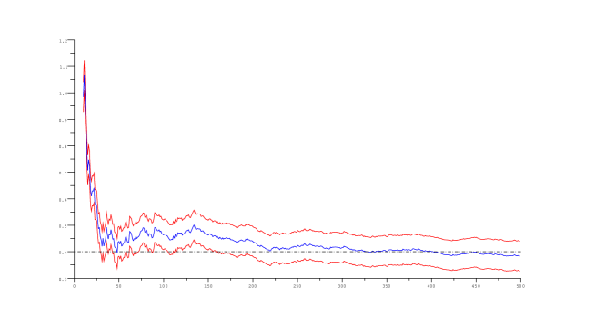
Figure 1: GPH estimator for ARFIMA(0,.4,0)

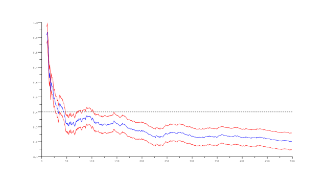
Figure 2: GPH estimator for ARFIMA(0,.4,0)+ noise

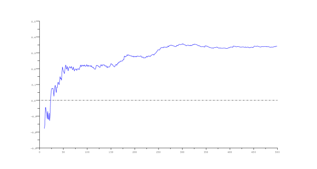
Figure 3: GPH “horror” plot

5 Technical results

Lemma 1

Let $\eta^{*}$ be a non decreasing slowly varying function on $(0,\pi]$ such that $\lim_{s\to 0}\eta^{*}(s)=0$. Let $\eta$ be a measurable function on $(0,\pi]$ such that $|\eta|\leq\eta^{*}$, and define $h(x)=-\int_{x}^{\pi}\frac{\eta(s)}{s}\,\mathrm{d}s$ and $h^{*}(x)=\int_{x}^{\pi}\frac{\eta^{*}(s)}{s}\,\mathrm{d}s$. Then, for any non decreasing sequence $m\leq n$,

$$\left|\sum_{k=1}^{m}\nu_{m}(k)h(x_{k})\right|\leq m\eta^{*}(x_{m})+O(\log^{2}(m)\eta^{*}(x_{m})+\log(m)h^{*}(x_{m})),$$ (12)

uniformly with respect to $|\eta|\leq\eta^{*}$.

Proof.  Since $\eta$ is slowly varying, the function $h$ is also slowly varying and satisfies $\lim_{x\to 0}\eta(x)/h(x)=0$. Then,

$$\sum_{k=1}^{m}h(x_{k}) =\frac{n}{2\pi}\int_{0}^{x_{m}}h(s)\,ds+\frac{n}{2\pi}\sum_{k=1}^{m}\int_{x_{k-1}}^{x_{k}}\{h(x_{k})-h(s)\}\,ds$$

$$=\frac{n}{2\pi}\int_{0}^{x_{m}}h(s)\,ds+\frac{n}{2\pi}\sum_{k=1}^{m}\int_{x_{k-1}}^{x_{k}}\int_{s}^{x_{k}}\frac{\eta(t)}{t}\,dt\,ds\;.$$

Thus, for $|\eta|\leq\eta^{*}$ and $\eta^{*}$ increasing,

$$\left|\sum_{k=1}^{m}h(x_{k})-\frac{n}{2\pi}\int_{0}^{x_{m}}h(s)\,ds\right| \leq\eta^{*}(x_{m})\frac{n}{2\pi}\sum_{k=1}^{m}\int_{x_{k-1}}^{x_{k}}\int_{s}^{x_{k}}\frac{dt}{t}\ ds$$

$$=\eta^{*}(x_{m})\left\{\sum_{k=1}^{m}\log(x_{k})-\frac{n}{2\pi}\int_{0}^{x_{m}}\log(s)\,ds\right\}$$

$$=\eta^{*}(x_{m})\left\{\sum_{k=1}^{m}\log(k)-m\log(m)+m\right\}$$

$$=O(\eta^{*}(x_{m})\log(m))\;.$$

By definition, it holds that $xh^{\prime}(x)=\eta(x)$. Integration by parts yield

$$\frac{n}{2\pi}\int_{0}^{x_{m}}h(s)\,ds=mh(x_{m})-\frac{n}{2\pi}\int_{0}^{x_{m}}\eta(s)\,\mathrm{d}s\;.$$ (13)

Thus,

$$\sum_{k=1}^{m}h(x_{k})=mh(x_{m})-\frac{n}{2\pi}\int_{0}^{x_{m}}\eta(s)\,\mathrm{d}s+O(\log(m)\eta^{*}(x_{m}))\;.$$ (14)

Similarly, we have:

$$\sum_{k=1}^{m}h(x_{k})\log(x)=mh(x_{m})\log(x_{m})-\frac{n}{2\pi}\int_{0}^{x_{m}}\{\eta(s)\log(s)+h(s)\}\,\mathrm{d}x\\ +O(\log(m)\{\log(x_{m})\eta^{*}(x_{m})+h^{*}(x_{m})\})\;.$$ (15)

By definition of $\nu_{m}(k)$, we have:

$$\nu_{m}(k) =\log(k)-\frac{1}{m}\sum_{j=1}^{m}\log(j)=\log(x_{k})-\log(x_{m})+1+O\left(\frac{\log(m)}{m}\right).$$

Hence, applying (13), (14) and (15), we obtain

$$\sum_{k=1}^{m} \nu_{m}(k)h(x_{k})$$

$$=\sum_{k=1}^{m}\log(x_{k})h(x_{k})-\{\log(x_{m})-1+O(\log(m)/m)\}\sum_{k=1}^{m}h(x_{k})$$

$$=\frac{n}{2\pi}\int_{0}^{x_{m}}\eta(s)\{\log(x_{m})-\log(s)\}\,\mathrm{d}s$$

$$\ \ \ \ \ \ \ \ \ \ \ \ \ \ \ \ \ \ \ \ \ \ \ \ \ \ \ \ \ \ +O(\log(m)\{\eta^{*}(x_{m})\log(x_{m})+h^{*}(x_{m})\})\;.$$

Finally, since $|\eta|\leq\eta^{*}$ and $\eta^{*}$ is non decreasing, we obtain

$$\frac{n}{2\pi}\left|\int_{0}^{x_{m}}\eta(s)\{\log(x_{m})-\log(s)\}\,ds\right|\\ \leq\frac{n}{2\pi}\eta^{*}(x_{m})\int_{0}^{x_{m}}\int_{s}^{x_{m}}\frac{1}{t}\,dt\,ds=m\eta^{*}(x_{m}).$$

This yields (12). ∎

Lemma 2

Let $\eta^{*}$ be a non decreasing slowly varying function such that $\lim_{x\to 0}\eta^{*}(x)=0$. Let $X$ be a Gaussian process with spectral density $f(x)=x^{-\alpha}L(x)$, where $\alpha\in[-\delta,\delta]$ and $L\in SV(\eta^{*})$. Let $\gamma=0,577216...$ denote Euler’s constant. Then, for all $n$ and all $k,j$ such that $0<x_{k},\,x_{j}\leq\pi/2$,

$$\left|\mathbb{E}[\log(\mathcal{E}_{k})]-\gamma\right|+\left|\mathbb{E}[\log^{2}(\mathcal{E}_{k})]-\frac{\pi^{2}}{6}\right|\leq C(\delta,\eta^{*})\log(1+k)k^{-1},$$

$$|\mathbb{E}[\log(\mathcal{E}_{k})-\gamma)(\log(\mathcal{E}_{j})-\gamma)]|\leq C(\delta,\eta^{*})\log^{2}(j)k^{-2}.$$

Proof of Lemma 2

It is well known (see for instance Hurvich et al. (1998), Moulines and Soulier (1999), Soulier (2001)) that the bounds of Lemma 2 are consequences of the covariance inequality for functions of Gaussian vectors of (Arcones, 1994, Lemma 1) and of the following bounds. For all $n$ and all $k,j$ such that $0<|x_{k}|\leq|x_{j}|\leq\pi/2$,

$$|\mathrm{cov}(d_{X,k},d_{X,j})|+|\mathrm{cov}(d_{X,k},\bar{d}_{X,j})-f(x_{k})\delta_{k,j}|\\ \leq C(\delta,\eta^{*})\sqrt{f(x_{k})f(x_{j})}\,\log(j)\,k^{-1}\;.$$

Such bounds have been obained when the spectral density is second order regularly varying. We prove these bounds under our assumptions that do not imply second order regular varition. Denote $D_{n}(x)=(2\pi n)^{-1/2}\sum_{t=1}^{n}\mathrm{e}^{-\mathrm{i}tx}$. Then

$$\mathrm{cov}(d_{X,k},d_{X,j})=\int_{-\pi}^{\pi}f(x)D_{n}(x_{k}-x)D_{n}(x_{j}+x)dx.$$

Recall that by definition of the class $SV(\eta^{*})$, there exists a function $\eta$ such that $|\eta|\leq\eta^{*}$ and $L(x)=L(\pi)\exp\{-\int_{x}^{\pi}s^{-1}\eta(s)\mathrm{d}s\}$. Since only ratio $L(x)/L(\pi)$ are involved in the bounds, without loss of generality, we can assume that $L(\pi)=1$. We first prove that for all $k$ such that $x_{k}\leq\pi/2$,

$$\left|\int_{-\pi}^{\pi}\left(\frac{f(x)}{f(x_{k})}-1\right)|D_{n}(x_{k}-x)|^{2}\,\mathrm{d}x\right|\leq C(\delta,\eta^{*})\log(k)k^{-1}\;.$$ (16)

Since $L\in SV(\eta^{*})$, the functions $x^{\epsilon}L(x)$ and $x^{\epsilon}L^{-1}(x)$ are bounded for any $\epsilon>0$ and

$$\sup_{x\in[0,\pi]}x^{\delta}(L(x)+L^{-1}(x))\leq C(\eta^{*},\delta)\;,$$ (17)

$$\sup_{\alpha\in[-1+\delta,1-\delta]}\int_{-\pi}^{\pi}f(x)\,\mathrm{d}x\leq C(\eta^{*},\delta)\ .$$ (18)

Since $\eta^{*}$ is increasing, for all $0<x<y\leq\pi/2$, it holds that

$$|f(x)-f(y)| =|x^{-\alpha}L(x)-y^{-\alpha}L(y)|$$

$$\leq\int_{x}^{y}|\alpha-\eta(s)|s^{-\alpha-1}L(s)\,\mathrm{d}s$$

$$\leq\int_{x}^{y}(1+\eta^{*}(\pi))s^{-\alpha-1}L(s)\,\mathrm{d}s\;.$$

Since $\alpha\in[-1+\delta,1-\delta]$, $x^{-\alpha-1}L(x)$ is decreasing. Hence

$$|f(x)-f(y)|\leq C(\eta^{*},\delta)x^{-1}f(x)(y-x)\;.$$ (19)

Define $F_{n}(x)=|D_{n}(x)|^{2}$ (the Fejer kernel). We have

$$\sup_{\pi/2\leq|x|\leq\pi}|F_{n}(x_{k}-x)|=O(n^{-1})\;,\ \ \ \ \int_{-\pi}^{\pi}F_{n}(x)\,\mathrm{d}x=1\;,$$ (20)

$$\int_{-\pi}^{\pi}D_{n}(y+x)D_{n}(z-x)\,\mathrm{d}x=(2\pi n)^{-1/2}D_{n}(y+z)\;.$$ (21)

From now on, $C$ will denote a generic constant which depends only on $\eta^{*}$, $\delta$ and numerical constants, and whose value may change upon each appearance. Applying (17), (18) and (20), we obtain

$$\int_{\pi/2\leq|x|\leq\pi}\left|f^{-1}(x_{k})f(x)-1\right|F_{n}(x-x_{k})\,\mathrm{d}x\leq Cn^{-1}(f^{-1}(x_{k})+1)\leq Ck^{-1}\;.$$

The integral over $[-\pi/2,\pi/2]$ is split into integrals over $[-\pi/2,-x_{k}/2]\cup[2x_{k},\pi/2]$, $[-x_{k}/2,x_{k}/2]$ and $[x_{k}/2,2x_{k}]$. If $x\in[-\pi/2,-x_{k}/2]\cup[2x_{k},\pi/2]$, then $F_{n}(x-x_{k})\leq Cn^{-1}x^{-2}$. Hence, applying Karamata’s Theorem (cf. (Bingham et al., 1989, Theorem 1.5.8)), we obtain:

$$\int_{-\pi/2}^{-x_{k}/2} +\int_{-\pi/2}^{-x_{k}/2}f(x)F_{n}(x)\,\mathrm{d}x$$

$$\leq Cn^{-1}\int_{x_{k}/2}^{\pi/2}x^{-\alpha-2}L(x)\,\mathrm{d}x\leq Cn^{-1}x_{k}^{-\alpha-1}L(x_{k})\leq Ck^{-1}f(x_{k})\;,$$

$$\int_{-\pi/2}^{-x_{k}/2} +\int_{-\pi/2}^{-x_{k}/2}F_{n}(x)\,\mathrm{d}x\leq Cn^{-1}\int_{x_{k}/2}^{\infty}x^{-2}\,\mathrm{d}x\leq Cn^{-1}x_{k}^{-1}\leq Ck^{-1}\;.$$

For $x\in[-x_{k}/2,x_{k}/2]$, $F_{n}(x_{k}-x)\leq n^{-1}x_{k}^{-2}$. Thus, applying again Karamata’s Theorem, we obtain:

$$\int_{-x_{k}/2}^{x_{k}/2}f(x)F_{n}(x-x_{k})\,\mathrm{d}x \leq Cn^{-1}x_{k}^{-2}\int_{-x_{k}/2}^{x_{k}/2}x^{-\alpha}L(x)\,\mathrm{d}x$$

$$\leq Cn^{-1}x_{k}^{-2}x_{k}^{-\alpha+1}L(x_{k})\leq Ck^{-1}f(x_{k})\;,$$

$$\int_{-x_{k}/2}^{x_{k}/2}F_{n}(x-x_{k})dx \leq Cn^{-1}x_{k}^{-1}\leq Ck^{-1}\;.$$

Applying (19) and the bound $\int_{-x_{k}/2}^{x_{k}}|x|F_{n}(x)|\,\mathrm{d}x\leq Cn^{-1}\log(k)$, we obtain:

$$\int_{x_{k}/2}^{2x_{k}}|f(x)-f(x_{k})|F_{n}(x-x_{k})\,\mathrm{d}x\\ \leq Cx_{k}^{-\alpha-1}L(x_{k}/2)\int_{x_{k}/2}^{2x_{k}}|x-x_{k}|F_{n}(x-x_{k})|\,\mathrm{d}x\leq Cf(x_{k})k^{-1}\log(k)\;.$$

This proves (16). We now prove that all $k,j$ such that $0<x_{k}\neq|x_{j}|\leq\pi/2$,

$$\left|\int_{-\pi}^{\pi}\left(\frac{f(x)}{f(x_{k})}-1\right)D_{n}(x_{k}-x)\overline{D_{n}(x_{j}-x)}\,\mathrm{d}x\right|\\ +\left|\int_{-\pi}^{\pi}\left(\frac{f(x)}{f(x_{k})}-1\right)D_{n}(x_{k}-x)D_{n}(x_{j}-x)\,\mathrm{d}x\right|\\ \leq C(\delta,\eta^{*})\log(k\vee|j|)(k\wedge|j|)^{-1}.$$ (22)

Define $E_{n,k,j}(x):=D_{n}(x_{k}-x)\overline{D_{n}(x_{j}-x)}$. Since $0\leq x_{k},x_{j}\leq\pi/2$, for $\pi/2\leq|x|\leq\pi$, we have $|E_{n,k,j}(x)|\leq Cn^{-1}$. Hence, as above,

$$\int_{\pi/2\leq|x|\leq\pi}|f^{-1}(x_{k})f(x)-1|\,\mathrm{d}x\leq Cn^{-1}(x_{k}^{\alpha}L^{-1}(x_{k})+1)\leq Ck^{-1}.$$

We first consider the case $k<j$ and we split the integral over $[-\pi/2,\pi/2]$ into integrals over $[-\pi/2,-x_{k}/2]\cup[2x_{j},\pi/2]$, $[-x_{k}/2,x_{k}/2]$, $[x_{k}/2,(x_{k}+x_{j})/2]$, $[(x_{k}+x_{j})/2,2x_{j}]$, denoted respectively $I_{1}$, $I_{2}$, $I_{3}$ and $I_{4}$.
$\bullet$ The bound for the integral over $[-\pi/2,-x_{k}/2]\cup[2x_{j},\pi/2]$ is obtained as above (in the case $k=j$) since $|E_{n,k,j}|\leq Cn^{-1}x^{-2}$. Hence $|I_{1}|\leq Ck^{-1}$.
$\bullet$ For $x\in[-x_{k}/2,x_{k}/2]$, $|E_{n,k,j}(x)|\leq Cn^{-1}x_{k}^{-2}$, hence we get the same bound: $|I_{2}|\leq Ck^{-1}$.
$\bullet$ To bound $I_{3}$, we note that on the interval $[x_{k}/2,(x_{k}+x_{j})/2]$,

$$|E_{n,k,j}(x)|\leq Cn^{1/2}(j-k)|D_{n}(x-x_{k})|,$$

and $n^{1/2}|x-x_{k}||D_{n}(x-x_{k}|$ is uniformly bounded. Hence, applying (19), we obtain

$$|I_{3}|\leq C(j-k)^{-1}x_{k}^{-1}x_{j}\leq Ck^{-1}.$$

$\bullet$ The bound for $I_{4}$ is obtained similarly: $|I_{4}|\leq Ck^{-1}\log(j)$.

$\bullet$ To obtain the bound in the case $x_{j}<x_{k}$, the interval $[-\pi,\pi]$ is split into $[-\pi,-\pi/2]\cup[\pi/2\pi]$ $[-\pi/2,-x_{k}/2]\cup[2x_{k},\pi/2]$, $[-x_{k}/2,x_{j}/2]$, $[x_{j}/2,(x_{k}+x_{j})/2]$ and $[(x_{k}+x_{j})/2,2x_{k}]$. The arguments are the same except on the interval $[-x_{k}/2,x_{j}/2]$ where a slight modification of the argument is necessary. On this interval, it still holds that $|E_{n,k,j}(x)|\leq n^{-1}x_{k}^{-2}$. Moreover, $x^{\delta}L(x)$ can be assumed increasing on $[0,x_{k}/2]$, and we obtain:

$$\int_{-x_{k}/2}^{x_{j}/2}x^{-\alpha}L(x)\,\mathrm{d}x\leq x_{k}^{\delta}L(x_{k})\int_{-x_{k}/2}^{x_{j}/2}x^{-\alpha-\delta}\,\mathrm{d}x\leq Cx_{k}^{-\alpha+1}L(x_{k})\;.$$

The rest of the argument remains unchanged.

$\bullet$ To obtain the bound in the case $x_{j}<0<x_{k}$, the interval $[-\pi,\pi]$ is split into $[-\pi,-\pi/2]\cup[\pi/2,\pi]$ $[-\pi/2,2x_{j}]\cup[2x_{k},\pi/2]$, $[2x_{j},-x_{k}/2]$, $[-x_{k}/2,x_{k}/2]$ and $[x_{k}/2,2x_{k}]$ and the same arguments are applied. ∎

References

- Arcones (1994) Miguel A. Arcones. Limit theorems for nonlinear functionals of a stationary Gaussian sequence of vectors. The Annals of Probability, 22(4):2242–2274, 1994.
- Bingham et al. (1989) Nick H. Bingham, Charles M. Goldie, and Jef L. Teugels. Regular variation, volume 27 of Encyclopedia of Mathematics and its Applications. Cambridge University Press, Cambridge, 1989.
- Drees (1998) Holger Drees. Optimal rates of convergence for estimates of the extreme value index. The Annals of Statistics, 26, 1998.
- Geweke and Porter-Hudak (1983) John Geweke and Susan Porter-Hudak. The estimation and application of long memory time series models. Journal of Time Series Analysis, 4(4):221–238, 1983.
- Giraitis et al. (1997) Liudas Giraitis, Peter M. Robinson, and Alexander Samarov. Rate optimal semiparametric estimation of the memory parameter of the Gaussian time series with long range dependence. Journal of Time Series Analysis, 18:49–61, 1997.
- Hall and Welsh (1984) Peter Hall and Alan H. Welsh. Best attainable rates of convergence for estimates of parameters of regular variation. The Annals of Statistics, 12(3):1079–1084, 1984.
- Hurvich and Ray (2003) Clifford M. Hurvich and Bonnie K. Ray. The local whittle estimator of long-memory stochastic volatility. Journal of Financial Econometrics, 1:445–470, 2003.
- Hurvich et al. (1998) Clifford M. Hurvich, Rohit Deo, and Julia Brodsky. The mean squared error of Geweke and Porter-Hudak’s estimator of the memory parameter of a long-memory time series. Journal of Time Series Analysis, 19, 1998.
- Hurvich et al. (2005) Clifford M. Hurvich, Eric Moulines, and Philippe Soulier. Estimating long memory in volatility. Econometrica, 73(4):1283–1328, 2005.
- Kuensch (1987) Hans R. Kuensch. Statistical aspects of self-similar processes. In Yu.A. Prohorov and V.V. Sazonov (eds), Proceedings of the first World Congres of the Bernoulli Society, volume 1, pages 67–74. Utrecht, VNU Science Press, 1987.
- Moulines and Soulier (1999) Eric Moulines and Philippe Soulier. Broadband log-periodogram regression of time series with long-range dependence. The Annals of Statistics, 27(4):1415–1439, 1999.
- Robinson (1995a) Peter M. Robinson. Gaussian semiparametric estimation of long range dependence. The Annals of Statistics, 23(5):1630–1661, 1995a.
- Robinson (1995b) Peter M. Robinson. Log-periodogram regression of time series with long range dependence. The Annals of Statistics, 23(3):1048–1072, 1995b.
- Soulier (2001) Philippe Soulier. Moment bounds and central limit theorem for functions of Gaussian vectors. Statistics & Probability Letters, 54(2):193–203, 2001.