The cost of being co-Büchi is nonlinear

Abstract

It is well known, and easy to see, that not each nondeterministic Büchi automaton on infinite words can be simulated by a nondeterministic co-Büchi automaton. We show that in the cases when such a simulation is possible, the number of states needed for it can grow nonlinearly. More precisely, we show a sequence of – as we believe, simple and elegant – languages which witness the existence of a nondeterministic Büchi automaton with $n$ states, which can be simulated by a nondeterministic co-Büchi automaton, but cannot be simulated by any nondeterministic co-Büchi automaton with less than $c*n^{7/6}$ states for some constant $c$. This improves on the best previously known lower bound of $3(n-1)/2$.

1 Introduction

1.1 Previous work

In 1962 Büchi was the first to introduce finite automata on infinite words. He needed them to solve some fundamental decision problems in mathematics and logic ([2], [6] [7]). They became a popular area of research due to their elegance and the tight relation between automata on infinite objects and monadic second-order logic. Nowadays, automata are seen as a very useful tool in verification and specification of nonterminating systems. This is why the complexity of problems concerning automata has recently been considered a hot topic (e. g. [5], [1]).

To serve different applications, different types of automata were introduced. In his proof of the decidability of the satisfiability of S1S, Büchi introduced nondeterministic automata on infinite words (NBW), which are a natural tool to model things that happen infinitely often. In a Büchi automaton, some of the states are accepting and a run on an infinite word is accepting if and only if it visits some accepting state infinitely often ([2]). Dually, a run of co-Büchi automaton (NCW) is accepting if and only if it visits non-accepting states only finitely often. There are also automata with more complicated accepting conditions – most well known of them are parity automata, Street automata, Rabin automata and Muller automata.

As in the case of finite automata on finite words, four basic types of transition relation can be considered: deterministic, nondeterministic, universal and alternating. In this paper, from now on, we only consider nondeterministic automata.

The problem of comparing the power of different types of automata is well studied and understood. For example it is easy to see that not every language that can be recognized by a Büchi automaton on infinite words (such languages are called $\omega$-regular languages) can be also recognized by a co-Büchi automaton. The most popular example of $\omega$-regular language that cannot be expressed by NCW is the language $L=\{w|w$ has infinitely many 0’s$\}$ over the alphabet $\{0,1\}$. On the other hand, it is not very hard to see that every language that can be recognized by a co-Büchi automaton is $\omega$-regular.

As we said, the problem of comparing the power of different types of automata is well studied. But we are quite far from knowing everything about the number of states needed to simulate an automaton of one type by an automaton of another type – see for example the survey [3] to learn about the open problems in this area.

In this paper we consider the problem of the cost of simulating a Büchi automaton on infinite words by a co-Büchi automaton (if such NCW exists), left open in [3]: given a number $n\in{\cal N}$, for what $f(n)$ can we be sure that every nondeterministic Büchi automaton with no more than $n$ states, which can be simulated by a co-Büchi automaton, can be simulated by a co-Büchi automaton with at most $f(n)$ states?

There is a large gap between the known upper bound and the known lower bound for such a translation. The best currently known translation goes via intermediate deterministic Street automaton, involving exponential blowup of the number of states ([8], [1]). More precisely, for NBW with $n$ states, we get NCW with $2^{O}(n\log n)$ states. For a long time the best known lower bound for $f$ was nothing more than the trivial bound $n$. In 2007 it was shown that there is an NBW with equivalent NCW such that there is no NCW equivalent to this NBW on the same structure ([4]). The first non-trivial (and the best currently known) lower bound is linear – the result of [1] is that, for each $n\in{\cal N}$, there exists a NBW with $n$ states such that there is a $NCW$ which recognizes the same language, but every such $NCW$ has at least $3(n-1)/2$ states.

There is a good reason why it is hard to show a lower bound for the above problem. The language (or rather, to be more precise, class of languages) used to show such a bound has to be hard enough to be expressed by a co-Büchi automaton, but on the other hand not too hard, because some (actually, most of) $\omega$-regular languages cannot be expressed by NCW at all. The idea given in the proof of $3(n-1)/2$ lower bound in [1], was to define a language which can be easily split into parts that can by recognized by a NBW but cannot by recognized by a NCW. The language they used was $L_{k}=\{w\in\{0,1\}^{\omega}|$ both $0$ and $1$ appear at least $k$ times in $w\}$. Let $L_{k}^{i}=\{w\in\{0,1\}^{\omega}|i$ appears infinitely often in $w$ and $(1-i)$ appear at least $k$ times in $w\}$, then it is easy to see that $L_{k}=L_{k}^{0}\cup L_{k}^{1}$, $L_{k}^{i}$ can be recognized by Büchi automata of size $k$ and $L_{k}^{i}$ cannot by recognized by any co-Büchi automaton. It is still, however, possible to built a NCW that recognizes $L_{k}$ with $3k+1$ states and indeed, as it was proved in [1], every NCW recognizing $L_{k}$ has at least $3k$ states.

1.2 Our contribution – a nonlinear lower bound

In this paper we give a strong improvement of the lower bound from [1]. We show that, for every integer $k$, there is a language $L_{k}$ such that $L_{k}$ can be recognized by an NBW with $\Theta(k^{2})$ states, whereas every NCW that recognizes this language has at least $\Theta(k^{7/3})$ states. Actually, the smallest NCW we know, which recognizes $L_{k}$, has $\Theta(k^{3})$ states, and we believe that this automaton is indeed minimal. In the terms of function $f$ from the above subsection this means that $f$ equals at least $cn^{7/6}$ for some $c$ (this is since $n$ is $\Theta(k^{2})$) and, if our conjecture concerning the size of a minimal automaton for $L_{k}$ is true, $f$ would equal at least $cn^{3/2}$ for some constant $c$.

The technical part of of this paper is organized as follows. In subsection 2.1 we give some basic definitions. In subsection 2.2 the definition of the language $L_{k}$ is presented. Also in this section we show how this language can be recognized by a Büchi automaton with $O(k^{2})$ states and how $L_{k}$ can be recognized by a co-Büchi automaton with $O(k^{3})$ states. The main theorem, saying that every co-Büchi automaton that recognizes $L_{k}$ has at least $\Theta(k^{7/3})$ states is formulated in the end of subsection 2.2 and the rest of the paper is devoted to its proof.

2 Technical Part

2.1 Preliminaries

A nondeterministic $\omega$-automaton is a quintuple $\langle\Sigma,Q,q_{0},\delta,\alpha\rangle$, where $\Sigma$ is an alphabet, $Q$ is a set of states, $q_{0}\in Q$ is an initial state, $\delta\subseteq Q\times\Sigma\times Q$ is a transition relation and $\alpha\subseteq Q$ is an accepting condition.

A run of $\omega$-automaton over a word $w=w_{1}w_{2}\dots$ is a sequence of states $q_{0}q_{1}q_{2}\dots$ such that for every $i\geq 0$, $q_{i}\in Q$ and $\langle q_{i},w_{i+1},q_{i+1}\rangle\in\delta$.

Depending on type of the automaton we we have different definitions of accepting run. For a Büchi automaton, a run is accepting, if it visits some state from accepting condition $\alpha$ infinitely often. In the case of a co-Büchi automaton, a run is accepting, if only states from the set $\alpha$ are visited infinitely often in this run. For a given nondeterministic $\omega$-automaton $\cal{A}$ and a given word $w$, we say that $\cal{A}$ accepts $w$ if there exists an accepting run of $\cal{A}$ on $w$. The words accepted by $\cal{A}$ form the language of $\cal{A}$, denoted by $L(\cal{A})$.

We say that a co-Büchi automaton ${\cal{A}}=\langle\Sigma,Q,q_{0},\delta,\alpha\rangle$ is in the normal form iff for each $\langle q,a,q^{\prime}\rangle\in\delta$ if $q$ is in $\alpha$, then also $q^{\prime}$ is in $\alpha$. Note that for a given NCW ${\cal{A}}=\langle\Sigma,Q,q_{0},\delta,\alpha\rangle$ the automaton ${\cal{A^{\prime}}}=\langle\Sigma,Q^{\prime},\langle q_{0},0\rangle,\delta^{\prime},\alpha\times\{1\}\rangle$, where $Q^{\prime}=Q\times\{0\}\cup\alpha\times\{1\}$ and $\delta^{\prime}=\{\langle\langle q,i\rangle,a,\langle q^{\prime},j\rangle\rangle\;|\;\langle q,a,q^{\prime}\rangle\in\delta\wedge i\leq j\wedge\langle q,i\rangle,\langle q^{\prime},j\rangle\in Q^{\prime}\}$ is in the normal form, recognizes the same language and has at most $2|Q|$ states.

For a given word $w=w_{1},w_{2},\dots$, let $w[i,j]=w_{i},w_{i+1},\dots,w_{j}$ and let $w[i,\infty]=w_{i},w_{i+1},\dots$.

An accepting run $q_{0},q_{1},\dots$ on a word $w=w_{1},w_{2},\dots$ of a co-Buchi automaton in the normal form is called shortest, if it reaches an accepting state as early as possible, that is if for each accepting run $p_{0},p_{1},\ldots$ of this automaton on $w$ it holds that if $p_{i}\in\alpha$ then also $q_{i}\in\alpha$.

2.2 Languages $L_{k}$ and their automata

Let $k\geq 64$ be a – fixed – natural number and let $\mathfrak{A}_{k}=\{1,2\ldots k\}$. The set $\Sigma_{k}=\{a,\bar{a}\;|\>a\in\mathfrak{A}_{2k}\}$ will be the alphabet of our language $L_{k}$.

Let us begin with the following informal interpretation of words over $\Sigma_{k}$. Each symbol $j\in\Sigma_{k}$ should be read as “agent $j$ makes a promise”. Each symbol $\bar{j}\in\Sigma_{k}$ should be read as “$j$ fulfills his promise”. The language $L_{k}$ consists (roughly speaking) of the words in which there is someone who at least $2k$ times fulfilled his promises, but there are also promises which were never fulfilled.

To be more formal:

Definition 1

For a word $w\in\Sigma_{k}^{\omega}$, where $w=w_{1}w_{2}\ldots$ and $i\in\cal N$, define the interpretation $h_{i}(w)$ as:

• $h_{i}(w)=\sharp$  if $w_{i}\in\mathfrak{A}_{2k}$ and $\bar{w_{i}}$ occurs in $w[i+1,\infty]$; (it is the fulfillment that counts, not a promise).

• $h_{i}(w)=0$ if $w_{i}\in\mathfrak{A}_{2k}$ and $\bar{w_{i}}$ does not occur in $w[i+1,\infty]$; (unfulfilled promises are read as 0).

• Suppose $w_{i}=\bar{s}$ for some $s\in\mathfrak{A}_{2k}$. Then $h_{i}(w)=s$ if there is $j<i$ such that $w_{j}=s$ and $\bar{s}$ does not occur in the word $w[j,i-1]$, and $h_{i}(w)=\sharp$ if there is no such $j$ (one first needs to make a promise, in order to fulfill it).

The interpretation $h(w)$ is now defined as the infinite word $h_{1}(w)h_{2}(w)\ldots$.

Now we are ready to formally define the language $L_{k}$:

Definition 2

$L_{k}$ is the set of such words $w\in\Sigma_{k}^{\omega}$ that:

• either there is at least one $0$ in $h(w)$ and there exists $s\in\mathfrak{A}_{2k}$ which occurs at least $2k$ times in $h(w)$,

• or there exists $i$ such that $h_{j}(w)=\sharp$ for all $j>i$.

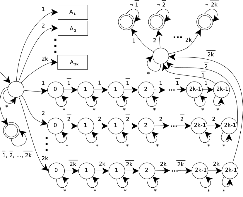
Figure 1: The $\omega$-automaton recognizing $L_{k}$ – all differences between NBW version and NCW version are in the body of $A_{i}$ (fig. 2). Label $\neg i$ stands (for better readability) for alternative of every label except $i$.

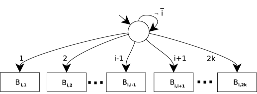
Figure 2: Automaton $A_{i}$ – the same for NBW and NCW, modulo the body of $B_{i,j}$ (fig. 3 for NBW and fig. 4 for NCW)

It is easy to see that each $w\in\Sigma_{k}^{\omega}$ satisfies at least one of the following three conditions: there is $s\in\mathfrak{A}_{2k}$ such that $h_{i}(w)=s$ for infinitely many numbers $i$, or there are infinitely many occurrences of $0$ in $h(w)$, or there is only a finite number of occurrences of symbols from $\mathfrak{A}_{2k}$ in $w$. Using this observation, we can represent $L_{k}$ in the following way:

$$L_{k} = \{viw\ |v\in\Sigma_{k}^{*}\wedge$$ (2)

$$( (i\in\mathfrak{A}_{2k}\wedge w\in(\Sigma_{k}\setminus\{\overline{i}\})^{\omega}\wedge\exists j\in\mathfrak{A}_{2k}\;\;h_{m}(viw)=j\text{ for infinitely many}$$

$$\text{ numbers }m)$$

$$\vee (i\in\mathfrak{A}_{2k}\wedge w\in(\Sigma_{k}\setminus\{\overline{i}\})^{\omega}\wedge\exists j\in\mathfrak{A}_{2k}\;\;h_{m}(viw)=j\text{ for at least }$$

$$2k\text{ numbers }m\text{ such that }m\leq|v|)$$

$$\vee (w\in\{\overline{1},\dots,\overline{2k}\}^{\omega}))\}$$ (3)

Figure 3: Automaton $B_{i,j}$ in the NBW case

Keeping in mind the above representation, it is easy to build a small NBW recognizing $L_{k}$ (see Figures 1, 2 and 3). The accepting state on the bottom left of Figure 1 checks if condition (3) is satisfied, and the other states (except of the states in the boxes $A_{i}$ and of the initial state) check if the condition (2) is satisfied. Reading the input $y$ the automaton first guesses the number $j$ from condition (2) and makes sure that $j$ occurs at least $2k$ times in $h(y)$. Then it guesses $i$ from condition (2), accepts, and remains in the accepting state forever, unless it spots $\bar{i}$. This part of the automaton works also correctly for the co-Büchi case.

The most interesting condition is (2). It is checked in the following way. At first, the automaton waits in the initial state until it spots $i$ from condition (2). Then, it goes to $A_{i}$, guesses $j$ and goes to the module $B_{i,j}$, which checks if $i$ does not occur any more, and if both $j$ and $\overline{j}$ occur infinitely often. This can be summarized as:

Theorem 2.1

Language $L_{k}$ can be recognized with a nondeterministic Büchi automaton with $\Theta(k^{2})$ states.

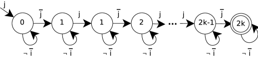
Figure 4: Automaton $B_{i,j}$ in the NCW case

Condition (2) cannot be checked by any NCW. However, it can be replaced by the condition

$$i\in\mathfrak{A}_{2k}\wedge w\in(\Sigma_{k}\setminus\{\overline{i}\})^{\omega}\wedge\exists j\in\mathfrak{A}_{2k}\;\;h_{m}(viw)=j\text{ for at least }2k\text{ numbers }m$$

which leads us to a NCW as on Figures 1, 2 and 4. In this case, automaton $B_{i,j}$ needs to count to $2k$, so it needs $\Theta(k)$ states. Therefore, the whole NCW automaton has $\Theta(k^{3})$ states. Actually, we believe that every NCW recognizing $L_{k}$ indeed needs $\Theta(k^{3})$ states.

Now we are ready to state our main theorem:

Theorem 2.2

Every NCW recognizing $L_{k}$ has at least $k\cdot\frac{k^{4/3}}{8}$ states.

The rest of this paper is devoted to the proof of this theorem. In subsection 2.3 we will define, for each co-Büchi automaton in the normal form, recognizing $L_{k}$ a family of $k$ disjoint sets of states, and in subsection 2.5 we will show that each such set has at least $\frac{k^{4/3}}{4}$ states. As we have seen in subsection 2.1, for a given NCW with $n$ states we can always build a NCW in the normal for with at most $2n$ states, which finally leads to $\frac{1}{2}\cdot k\cdot\frac{k^{4/3}}{4}$ lower bound.

2.3 The k disjoint sets of states

Let ${\cal A}=\langle\Sigma_{k},Q,q_{0},\delta,\alpha\rangle$ be an NCW in the normal form with $N$ states that recognizes $L_{k}$.

Let $w_{i,j}=i(j^{N}\overline{1},\overline{2},\dots,\overline{i-1},\overline{i+1},\dots,\overline{2k})^{\omega}$. For every $i\neq j$ let $q_{0}$, $q_{i,j}^{1}$, $q_{i,j}^{2}$, $q_{i,j}^{3},\dots$ be a fixed shortest accepting run of $\cal A$ on $w_{i,j}$.

Words $w_{i,j}$ will be the main tool in our attempt to fool the automaton if it has too few states so let us comment on their structure. First notice, that the $i$, the very first symbol of $w_{i,j}$, will turn into the only $0$ in $h(w)$ – this is, among other reasons, since for all $m\neq i$ the symbol $\overline{m}$ occurs infinitely many times in $w$. See also that if we replaced the blocks $j^{N}$ in the definition of $w_{i,j}$ by just a single $j$, then the word would still be in $L_{k}$ – since we do not count promises but fulfillments, the remaining $j$’s are almost redundant. It is only in the proof Lemma 4(ii) that we will need them. In the rest of the proof we will only be interested in one state of $A$ per each such block of symbols $j$. For this reason we define $block(l)=N+1+l(N+2k-1)$ as the function that points to the index of the state in run $q_{0},q_{i,j}^{1},q_{i,j}^{2},q_{i,j}^{3},\dots$ just after reading the $l$-th block $j^{N}$.

Let $Q_{i,j}=\{q_{i,j}^{block(c)}|c\in{\cal N}\}$.

Lemma 1

For every $i,j,m,l\in\mathfrak{A}_{2k}$ such that $m\neq i\neq j\neq l$ and $m\neq j$, the sets $Q_{i,m}$ and $Q_{j,l}$ are disjoint.

Proof

Suppose that there exist $i,j,m,l\in\mathfrak{A}_{2k}$, and $s,t\in{\cal N}$ such that $m\neq i\neq j\neq l$, $m\neq j$ and $q_{i,m}^{s}=q_{j,l}^{t}$. Let $v=w_{i,m}[0,block(s)].w_{j,l}[block(t)+1,\infty]$. This word is accepted by $\cal A$, because there exists an accepting run $q_{0}$, $q_{i,m}^{1}$, $\dots$ , $q_{i,m}^{block(s)},q_{j,l}^{block(t)+1},q_{j,l}^{block(t)+2},\dots$ of $\cal A$.

The only letters without the overline in $v$ are $i$, $m$ and $l$. However, the only overlined letter that does not occur infinitely often in $v$ is $\overline{j}$. This letter is different from $i$, $m$ and $l$ because of the assumptions we made. Therefore $0$ does not occur in $h(v)$ and $v\not\in L_{k}$.∎

We say that $l$ is huge if $l>k$ and that $l$ is small otherwise.

For every $i$ let $Q_{i}=\bigcup\{Q_{i,j}|j\text{ is small}\}$. A simple conclusion from Lemma 1 is that for each huge $i,j$ such that $i\neq j$ the sets $Q_{i}$ and $Q_{j}$ are disjoint. This implies, that Theorem 2.2 will be proved, once we prove the following lemma:

Lemma 2

For each huge $i\in\mathfrak{A}_{2k}$ the size of the set $Q_{i}$ is greater than $\frac{k^{4/3}}{4}$.

2.4 Combinatorial lemma

The $n\times m$ state matrix is a two-dimensional matrix with $n$ rows and $m$ columns. We say that $n\times m$ state matrix is $l$-painted if each of its cells is labeled with one of $l$ colors and the minimal distance between two cells in the same row and of the same color is at least $m$.

For a painted $n\times m$ state matrix, we say that an $M_{i,j}$ is a cell on the left border if $j=1$, and is on the right border if $j=m$. We say that $M_{i,j}$ is a successor of $M_{i^{\prime},j^{\prime}}$ if $i=i^{\prime}$ and $j=j^{\prime}+1$.

The path $w$ through a painted $n\times m$ state matrix $M$ is a sequence of cells $c_{1}$, $c_{2}$, $\dots$, $c_{z}$ such that $c_{1}$ is on the left border, $c_{z}$ is on the right border, and for each $s<z$ either $c_{s+1}$ is a successor of $c_{s}$ (we say that “there is a right move from $c_{s}$ to $c_{s+1}$”) or $c_{s}$ and $c_{s+1}$ are of the same color (we say that “there is a jump from $c_{s}$ to $c_{s+1}$”)

We say that a path $w$ is good, if there are no consecutive $k$ right moves in $w$, and no jump leads to (a cell in) a row that was already visited by this path. Notice that in particular a good path visits at most $k$ cells in any row.

Our main combinatorial tool will be:

Lemma 3

Let $M$ be an $\lfloor\frac{k^{4/3}}{4}\rfloor$-painted $k\times\lfloor\frac{k^{4/3}}{4}\rfloor$ state matrix. Then there exists a good path on $M$.

The proof of this lemma is left to subsection 2.6

2.5 From automaton to state matrix

We are now going to prove Lemma 2. Let a huge $i\in\mathfrak{A}_{2k}$ be fixed in this subsection and assume that $|Q_{i}|<\frac{k^{4/3}}{4}$. We will show that there exists a word $w$ such that $\cal A$ accepts $w$ and no agent fulfiles its promises at least $2k$ times in $w$.

Let $j$ be an small number from $\mathfrak{A}_{2k}$. Let us begin from some basic facts about $Q_{i,j}$:

Lemma 4

1. There exists a number $l$ such that for every $s<l$ the state $q_{i,j}^{block(s)}$ is not in $\alpha$ and for every $s\geq l$ the state $q_{i,j}^{block(s)}$ is in $\alpha$. Define $acc(i,j)=l$.

2. No accepting state from $Q_{i}$ can be reached on any run of $A$ before some agent fulfilled its promises $2k-1$ times. It also implies that $acc(i,j)\geq 2k-1$.

3. The states $q_{i,j}^{block(0)},q_{i,j}^{block(1)},\dots,q_{i,j}^{block(acc(i,j))}$ are pairwise different.

Proof

1. This is since $\cal A$ is in the normal form.

2. While reading a block of $N$ symbols $j$, the automaton is in $N+1$ states, so there is a state visited at least twice. If this state was accepting, then a pumping argument would be possible – we could simply replace the suffix of the word after this block with the word $j^{\omega}$ and the new word would still be accepted, despite the fact that it is not in $L_{k}$.

3. Suppose $q_{i,j}^{block(s)}$ and $q_{i,j}^{block(t)}$ are equal and non-accepting. For every $s<t\leq acc(i,j)$, the words $w_{i,j}[block(s)+1,\infty]$ and $w_{i,j}[block(t)+1,\infty]$ are identical. Then a pumping argument works again – we can find a shorter accepting run by pumping out the states $q_{i,j}^{block(s)},\dots,q_{i,j}^{block(t)-1}$. But this contradicts the assumption that our run is shortest.∎

We want to show that $|Q_{i}|\geq\frac{k^{4/3}}{4}$. If for any small $j$ there is $acc(i,j)\geq\frac{k^{4/3}}{4}-1$ then, thanks to Lemma 4(iii) we are done. So, for the rest of this subsection, we assume that $acc(i,j)<\frac{k^{4/3}}{4}-1$ for each small $j$.

We will now construct a $\lfloor\frac{k^{4/3}}{4}\rfloor$ - painted $k\times\lfloor\frac{k^{4/3}}{4}\rfloor$ state matrix $M$ in such a way, that its $m$’th row will, in a sense, represent the accepting run on the word $w_{i,m}$. More precisely, take a $k\times\lfloor\frac{k^{4/3}}{4}\rfloor$ matrix $M$ and call the cells $M_{m,j}$ of $M$, where $j\leq acc(i,m)$, real cells and call the cells $M_{m,j}$ of $M$ with $j>acc(i,m)$ ghosts. For a ghost cell $M_{m,j}$ and the smallest natural number $l$ such that $j-lk\leq acc(i,m)$ call the real cell $M_{(}m,j-lk)$ the host of $M_{m,j}$. Notice that each ghost has its host, since, by Lemma 4 (ii), $acc(i,m)\geq 2k-1$, which means that there are at least $k$ real cells in each row.

If $M_{m,j}$ is real then define its color as $q_{i,m}^{block(j-1)}$. If $M_{m,j}$ is a ghost then define its color as the color of its host. Now see that $M$ is indeed a $\lfloor\frac{k^{4/3}}{4}\rfloor$ - painted $k\times\lfloor\frac{k^{4/3}}{4}\rfloor$ state matrix – the condition concerning the shortest distance between cells of the same color in the same row of $M$ is now satisfied by Lemma 4 (iii) and the condition concerning the number of colors is satisfied, since we assume that $|Q_{i}|\leq\frac{k^{4/3}}{4}$.

By Lemma 3 we know that there is a good path in $M$. This means that Lemma 2 will be proved once we show:

Lemma 5

If there exists a good path in $M$, then there exists a word $w\not\in L_{k}$ such that $w$ is accepted by $\cal A$.

Proof

Suppose $r$ is a good path in $M$ and $c$ is the first ghost cell on $r$. Let $c^{\prime}$ be the direct predecessor of $c$ on $r$. If the move from $c^{\prime}$ to $c$ was a right move then define a new path $p$ as the prefix of $r$ ending with $c$. If the move from $c^{\prime}$ to $c$ was a jump, then suppose $c^{\prime\prime}$ is the host of $c$, and define $p$ as the following path: first take the prefix of $r$ ending with $c^{\prime}$. Then jump to $c^{\prime\prime}$ (it is possible, since the color of a ghost is the color of its host). Then make at most $k-1$ right moves to the last real cell in this row.

It is easy to see that $p$ satisfies all the conditions defining a good path, except that it does not reach the right border of $M$.

Let $p$ be a concatenation of words $p_{1}$,$p_{2}\ldots$,$p_{z}$, such that each move between $p_{x}$ and $p_{x+1}$ is a jump but there are no jumps inside any of $p_{x}$. This means that each $p_{x}$ is contained in some row of $M$, let $\beta(x)$ be a number of this row. This also means, since $p$ is (almost) a good path, that $|p_{x}|\leq k$ for each $x$.

Let $v_{i}=\overline{1},\overline{2},\dots,\overline{i-1},\overline{i+1},\dots$, $\overline{2k}$. Now define an infinite word $w$ as follows:

$$w=i\beta(1)^{N}(v_{i}\beta(1)^{N})^{|p_{1}|-1}(v_{i}\beta(2)^{N})^{|p_{2}|-1}\ldots(v_{i}\beta(z)^{N})^{|p_{z}|-1}\beta(z)^{\omega}$$

To see that $w\not\in L_{k}$ notice, that a symbol $s\in\mathfrak{A}_{2k}$ occurs in $h(w)$ only if $s=\beta(x)$ for some $x\in\{1,2\ldots z\}$ and that it occurs at most $|p_{x}|+1\leq k$ times in $w$. The fact that $A$ accepts $w$ follows from the construction of path $p$ and from Lemma 4 (ii).∎

2.6 Proof of the combinatorial lemma

Let $n=\lfloor\frac{k^{4/3}}{4}\rfloor$ and $M$ be an $n$-painted $k\times n$ state matrix. We split the matrix $M$ into matrices $M^{0},M^{1},...,M^{\lceil\frac{2n}{k}\rceil-1}$, each of them of $k$ rows and each of them (possibly except of the last one) of $\frac{k}{2}$ columns, such that $M^{i}$ contains columns $i\frac{k}{2}+1,i\frac{k}{2}+2\dots,min(i\frac{k}{2}+\frac{k}{2},n)$. The matrices $M^{0},M^{1},...,M^{\lceil\frac{2n}{k}\rceil-2}$ will be called multicolumns.

We are going to build a path $w=c_{1}c_{2}\ldots c_{z}$ through $M$ satisfying the following:

• if $w$ has a jump from $c_{j}$ to $c_{j+1}$ then both $c_{j}$ and $c_{j+1}$ belong to the same multicomumn;

• $w$ has exactly ${\lceil\frac{2n}{k}\rceil-1}$ jumps, one in each multicolumn;

• no jump on $w$ leads to a previously visited row of $M$.

Clearly, such a path will be a good path. This is since the width of each multicolumn is $\frac{k}{2}$, and each sequence of consecutive right moves on $w$ will be contained in two adjacent multicolumns (except of the last such sequence, which is contained in the last multicolumn and $M^{\lceil\frac{2n}{k}\rceil-1}$).

Let $s=\frac{k^{1/3}}{2}$. Since $\lceil s\rceil=\lceil\frac{2\cdot k^{4/3}/4}{k}\rceil\geq\lceil\frac{2n}{k}\rceil$, the number $\lceil s\rceil-1$ is not smaller than the number of jumps we want to make.

Now we concentrate on a single multicolumn $M^{i}$, which is a matrix with $k$ rows and with $\frac{k}{2}$ columns. We will call two rows of such a multicolumn brothers if at least one cell of one of those rows is of the same color as at least one cell of another (i.e. two rows are brothers if a path through $M^{i}$ can make a jump between them).

Suppose some of the rows of the multicolumn $M^{i}$ belong to some set $D^{i}$ of dirty rows. The rows which are not dirty will be called clean. A color will be called clean if it occurs in some of the clean rows. A row will be called poor if it has less than $\lceil s\rceil$ clean brothers. One needs to take care here – in the following procedure, while more rows will get dirty, more rows will also get poor:

Procedure (Contaminate a single multicolumn($D^{i}$,$M^{i}$) )
while there are clean poor rows (with respect to the current set $D^{i}$ of dirty rows) in $M^{i}$, select any clean poor row and all his brothers, and make them dirty (changing $D^{i}$ accordingly).
end of procedure

We would like to know how many new dirty rows can be produced as a result of an execution of the above procedure.

Each execution of the body of the while loop makes dirty at most $\lceil s\rceil$ rows and decreases the number of clean colors by at least $\frac{k}{2}$ – none of the colors of the selected clean poor row remains clean after the body of the while loop is executed. Since there are at most $n$ colors in the multicolumn (as $M$ is $n$-colored), the body of the while loop can be executed at most $\frac{n}{k/2}\leq\lceil s\rceil$ times, which means that at most $\lceil s\rceil^{2}$ new dirty rows can be produced.

Notice that after an execution of the procedure, none of the clean rows is poor.

Now we are ready for the next step:

Procedure (Contaminate all multicolumns)
         Let $D^{\lceil\frac{2n}{k}\rceil-1}=\emptyset$;
         for $i=\lceil\frac{2n}{k}\rceil-2$ down to 0
                  Let $D^{i}=D^{i+1}$;
                  Contaminate a single multicolumn($D^{i}$,$M^{i}$);
end of procedure

We used a convention here, that a set $D^{i}$ of rows is identified with the set of numbers of those rows. Thanks to that we could write the first line of the above procedure, saying “consider the dirty rows of $M^{i+1}$ to be also dirty in $M^{i}$”.

Suppose $D^{0},D^{1}\ldots D^{\lceil\frac{2n}{k}\rceil-2}$ are sets of dirty rows in multicolumns $M^{0}$,$M^{1}$, $\ldots$, $M^{\lceil\frac{2n}{k}\rceil-2}$ resulting from an execution of the procedure Contaminate all multicolumns. Notice, that for each $0\leq i\leq\lceil\frac{2n}{k}\rceil-2$ the inclusion $D^{i+1}\subseteq D^{i}$ holds. In other words, if a row is clean in $M^{i}$, then it is also clean in $M^{i+1}$.

The following lemma explains why clean rows are of interest for us:

Lemma 6

Suppose $w=c_{1}c_{2}\ldots c_{z}$ is a path through the matrix consisting of the first $i$ multicolumns of $M$ (or, in other words, of the first $\frac{ki}{2}$ columns of $M$). Suppose (i) $w$ has exactly one jump in each multicolumn, and each jump leads to a row which was not visited before, (ii) if there is a jump from $c_{j}$ to $c_{j+1}$ then both $c_{j}$ and $c_{j+1}$ belong to the same multicomumn. Suppose finally, that (iii) the cell where $w$ reaches the right border of the matrix, belongs to a clean row $r$. Then $w$ can be extended to a path through the matrix consisting of the first $i+1$ multicolumns of $M$, in such a way that this extended path will also satisfy conditions (i)-(iii).

Proof

The only thing that needs to be proved is that one can jump, in multicolumn $M^{i}$, from row $r$ to some clean row which was not visited before. Since, by assumption, $r$ was clean in $M^{i-1}$, it is also clean in $M^{i}$. Since there are no clean poor rows in $M^{i}$, we know that $r$ has at least $\lceil s\rceil$ clean brothers. At most $i$ of them were visited so far by the path, where of course $i\leq\lceil s\rceil-1$.∎

Now, starting from an empty path and a clean row in $M^{0}$ and using the above lemma $\lceil\frac{2n}{k}\rceil-2$ times we can construct a path $w$ as described in the beginning of this subsection and finish the proof of Lemma 3. The only lemma we still need for that is:

Lemma 7

$|D^{0}|<k$. In other words, there are clean rows in $M^{0}$.

Proof

Let $l=\lceil s\rceil-2$ be the index of the last multicolumn. The number of dirty rows in $D^{l-i}$ can be bounded by $(i+1)\cdot\lceil s\rceil^{2}$ because of observations about defined procedures. For $i=l$, we have $(\lceil s\rceil-1)\cdot\lceil s\rceil^{2}$, what is not greater then $s(s+1)^{2}=\frac{k^{1/3}}{2}(\frac{k^{1/3}}{2}+1)^{2}$ which is, finally, less then $k$, because $k\geq 8$.∎

References

- [1] B. Aminof and O. Kupferman and O. Lev. On the Relative Succinctness of Nondeterministic Büchi and co-Büchi Word Automata. In In Proc. of the 15th Int. Conf. on Logic for Programming, Artificial Intelligence, and Reasoning, LNCS 5330, pages 183–197. Springer, 2008.
- [2] J.R. Büchi. On a decision method in restricted second order arithmetic. In Proc. Int. Congress on Logic, Method, and Philosophy of Science. 1960, pages 1–12. Stanford University Press, 1962.
- [3] O. Kupferman. Tightening the exchange rate beteen automata. In Proc. 16th Annual Conf. of the European Association for Computer Science Logic, LNCS 4646, pages 7–22, 2007.
- [4] O. Kupferman, G. Morgenstern, and A. Murano. Typeness for -regular automata. In 2nd Int. Symp. on Automated Technology for Verification and Analysis, LNCS 3299, pages 324–338. Springer, 2004.
- [5] O. Kupferman, M. Vardi. Weak Alternating Automata Are Not That Weak. In Proceedings of the Fifth Israel Symposium on the theory of Computing Systems (ISTCS ’97) (June 17 - 19, 1997). ISTCS. IEEE Computer Society, Washington, DC, 147.
- [6] R. McNaughton. Testing and generating infinite sequences by a finite automaton. Information and Control, 9:521–530, 1966.
- [7] M.O. Rabin. Decidability of second order theories and automata on infinite trees. Transaction of the AMS, 141:1–35, 1969.
- [8] S. Safra. On the complexity of -automata. In Proc. 29th IEEE Symp. on Foundations of Computer Science, pages 319–327, 1988.