Entanglement for a bimodal cavity field interacting with a two-level atom

Abstract

Negativity has been adopted to investigate the entanglement in a system composed of a two-level atom and a two-mode cavity field. Effects of Kerr-like medium and the number of photon inside the cavity on the entanglement are studied. Our results show that atomic initial state must be superposed, so that the two cavity field modes can be entangled, moreover, we also conclude that the number of photon in the two cavity mode should be equal. The interaction between modes, namely, the Kerr effect, has a significant negative contribution. Note that the atom frequency and the cavity frequency have an indistinguishable effect, so a corresponding approximation has been made in this article. These results may be useful for quantum information in optics systems.

Keywords: Negativity; Kerr-like medium; Jaynes-Cummings model.

Quantum computation, one of the most fascinating applications of quantum mechanics, has the potential to outperform their classical counterparts in solving hard problems using much less time. There has been an ongoing effort to search for various physical systems that maybe propitious to implement quantum computation. Several prospective approaches for scalable quantum computation have been identified 1 ; 2 ; 3 ; 4 . Compared to other physical systems, the optic quantum can be easily realized in experiments. In quantum optics, the Jaynes-Cummings (JC) model is one of the exactly solvable models describing the interaction between a single-mode radiation field and a two-level atom. It has been realized experimentally in 1987 5 . There are many ongoing experimental and theoretical investigations on the various extensions of the JC model, such as a bimodal cavity field 6 ; 7 , two atoms 8 ; 9 , multilevel atoms 10 ; 11 , and so on. A two-level atom interacting with a two-mode cavity field is discussed here.

In view of the resource character of the entanglement, more attention has been paid to its quantification, such as the concurrence, the negativity, the relative entropy of entanglement etc. Entanglement between two qubits in arbitrary state has been quantified by concurrence 12 ; 13 ; 14 . It is generally considered that the two-atomic Wehrl entropy 15 can be used to quantify the entanglement in the JC model when these modes are initially prepared in the maximally entangled states 16 ; 17 . Here we use negativity as the measure and deal with the mixed state entanglement 18 . Many efforts have been put on the study of the two-mode JC model, but Kerr effect 19 ; 20 ; 21 ; 22 has not been considered, and this is the main motivation of the present paper. The scaled units are used in this work. The interaction between the field and atom are considered in an ideal and closed cavity, namely, the field damping and the radioactive damping 23 are ignored.

The system we considered here is an effective two-level atom with upper and lower states denoted by $|\uparrow>$ and $|\downarrow>$, respectively. The corresponding frequencies are $\omega_{a}$ and $\omega_{b}$, moreover, we denote $\omega_{\alpha}$ as the transition frequency between states $|\uparrow>$ and $|\downarrow>$. In the two-photon processes, some intermediate states $|i>$, i=c, d,$\cdots$ are involved, which are assumed to be coupled to $|\uparrow>$ and $|\downarrow>$ by dipole-allowed transition. Let $\omega_{i}$ denote the corresponding frequency of the atomic energy level $|i>$. There are two requirements: firstly, the atom interacts with the two cavity fields with frequencies $\omega_{1}$ and $\omega_{2}$, where $\omega_{1}$+ $\omega_{2}\cong\omega_{\alpha}$; secondly, $\omega_{a}-\omega_{i}$ and $\omega_{b}-\omega_{i}$ are off resonance of the one-photon linewidth with $\omega_{1}$ and $\omega_{2}$. If both are satisfied, then the intermediate states can be adiabatically eliminated 24 and the effective Hamiltonian of the system can be written in the rotating-wave approximation as 25 ; 26

$$H=\sum_{j=1}^{2}\omega_{j}a_{j}^{\dagger}a_{j}+\omega_{\alpha}\frac{\sigma_{z}}{2}+\chi(a_{1}^{{\dagger}2}a_{1}^{2}+a_{2}^{{\dagger}2}a_{2}^{2})+\lambda(a_{1}a_{2}\sigma_{+}+a_{1}^{{\dagger}}a_{2}^{{\dagger}}\sigma_{-}),$$ (1)

where $a_{j}^{{\dagger}}(a_{j})$ and $\omega_{j}$ denote the creation (annihilation) operator and frequency in the $j$th mode, the natural unit $\hbar=1$ is used throughout the paper. $\sigma_{\pm}=(\sigma_{x}\pm i\sigma_{y})/2$ is the raising and lowering operators, with $\sigma_{m}(m=x,y,z)$ is common Pauli spin operator. $\lambda$ is the coupling constant between the atom and the modes, known as the Rabi frequency. $\chi$ is the dispersive part of the third-order nonlinearity of the Kerr-like medium. Through out the investigation, we consider that $\omega_{1}+\omega_{2}=\omega_{\alpha}$ (i.e. the resonance case). After some study, it is found that the frequency of two modes have the same effect on negativity, so for simplicity, it is given that $\omega_{1}=\omega_{2}=\omega$ in the subsequent calculations.

We assume that the initial state of the system has the form of

$$|\Psi(0)\rangle=\cos\theta|n_{1},n_{2},\uparrow\rangle+\sin\theta|n_{1},n_{2},\downarrow\rangle,$$ (2)

where $n_{1}$ and $n_{2}$ are field quantum state in the Fock representation. Here different values of $\theta$ describe the states with different amplitudes. In view of the initial condition and Schrödinger equation, the wave function of the system at time $t$ can be obtained as

$$|\Psi(t)\rangle=a(t)|n_{1},n_{2},\uparrow\rangle+b(t)|n_{1},n_{2},\downarrow\rangle$$

$$\ \ \ \ \ \ \ \ \ +c(t)|n_{1}+1,n_{2}+1,\downarrow\rangle+d(t)|n_{1}-1,n_{2}-1,\uparrow\rangle,$$ (3)

under the condition $|a(t)|^{2}+|b(t)|^{2}+|c(t)|^{2}+|d(t)|^{2}=1$, and

$$a(t)=\frac{1}{2\xi_{1}}\{e^{-T(i\gamma_{1}+\xi_{1})}\cos\theta[i(e^{2T\xi_{1}}-1)\zeta(n_{1}+n_{2})+\xi_{1}(e^{2T\xi_{1}}+1)]\};$$

$$b(t)=\frac{1}{2\xi_{2}}\{e^{-T(i\gamma_{2}+\xi_{2})}\sin\theta[-i(e^{2T\xi_{2}}-1)\zeta(n_{1}+n_{2}-2)+\xi_{2}(e^{2T\xi_{2}}+1)]\};$$

$$c(t)=-\frac{1}{2\xi_{1}}[ie^{-T(i\gamma_{1}+\xi_{1})}\eta\cos\theta\sqrt{(1+n_{1})(1+n_{2})}];$$

$$d(t)=-\frac{1}{2\xi_{2}}[ie^{-T(i\gamma_{2}+\xi_{2})}\eta\sin\theta(e^{2T\xi_{2}}-1)\sqrt{n_{1}n_{2}}];$$

$$\xi_{1}=\sqrt{-\eta^{2}-\zeta^{2}n_{1}^{2}-n_{2}(\eta^{2}+\zeta^{2}n_{2}^{2})-n_{1}[\eta^{2}(1+n_{2})+2\zeta^{2}n_{2}]};$$

$$\xi_{2}=\sqrt{-\zeta^{2}n_{1}^{2}-\zeta^{2}(n_{2}-2)^{2}+n_{1}(4\zeta^{2}-n_{2}\eta^{2}-2\zeta^{2}n_{2})};$$

$$\gamma_{1}=1+n_{1}+n_{2}+\zeta(n_{1}^{2}+n_{2}^{2});$$

$$\gamma_{2}=-1+2\zeta+(1-2\zeta)n_{1}+\zeta n_{1}^{2}+n_{2}+\zeta(n_{2}-2)n_{2},$$ (4)

where $\eta=\lambda/\omega$, $\zeta=\chi/\omega$, and $T=\omega t$. From the above equations, the state density operator at time $t$, $\rho(t)=|\Psi(t)\rangle\langle\Psi(t)|$, can be easily derived.

If we know density matrix $\rho_{12}$ of a composite system composed of subsystem $1$ and $2$, the reduced density operator for subsystem $1$ is $\rho_{1}=Tr_{2}(\rho_{12})$. In our case, the density operator of two modes for a given atom state is $\rho_{f}(t)=Tr_{a}\rho(t)$ which can be found in the basis $\{|i,j\rangle,$ $i=n_{1}-1,$ $n_{1},$ $n_{1}+1$ and $j=n_{2}-1,$ $n_{2},$ $n_{2}+1\}$ as

$$\rho_{f}(t)=\left({{\begin{array}[]{*{20}c}\ \ \ {|d|^{2}\hfill}&{0\hfill}&{0\hfill}&{0\hfill}&{da^{*}\hfill}&{0\hfill}&{0\hfill}&{0\hfill}&{0\hfill\par}\\ \ \ \ {0\hfill}&{0\hfill}&{0\hfill}&{0\hfill}&{0\hfill}&{0\hfill}&{0\hfill}&{0\hfill}&{0\hfill}\\ \ \ \ {0\hfill}&{0\hfill}&{0\hfill}&{0\hfill}&{0\hfill}&{0\hfill}&{0\hfill}&{0\hfill}&{0\hfill}\\ \ \ \ {0\hfill}&{0\hfill}&{0\hfill}&{0\hfill}&{0\hfill}&{0\hfill}&{0\hfill}&{0\hfill}&{0\hfill}\\ \ \ \ {ad^{*}\hfill}&{0\hfill}&{0\hfill}&{0\hfill}&{|a|^{2}+|b|^{2}\hfill}&{0\hfill}&{0\hfill}&{0\hfill}&{bc^{*}\hfill}\\ \ \ \ {0\hfill}&{0\hfill}&{0\hfill}&{0\hfill}&{0\hfill}&{0\hfill}&{0\hfill}&{0\hfill}&{0\hfill}\\ \ \ \ {0\hfill}&{0\hfill}&{0\hfill}&{0\hfill}&{0\hfill}&{0\hfill}&{0\hfill}&{0\hfill}&{0\hfill}\\ \ \ \ {0\hfill}&{0\hfill}&{0\hfill}&{0\hfill}&{0\hfill}&{0\hfill}&{0\hfill}&{0\hfill}&{0\hfill}\\ \ \ \ {0\hfill}&{0\hfill}&{0\hfill}&{0\hfill}&{cb^{*}\hfill}&{0\hfill}&{0\hfill}&{0\hfill}&{|c|^{2}\hfill}\\ \end{array}}}\right),$$ (14)

which, generally speaking, is a mixed state. So we introduce negativity which is the usual measurement of entanglement for a mixed state and is defined as

$$N(\rho)\equiv\frac{\parallel\rho^{T_{A}}\parallel_{1}-1}{2},$$ (15)

where $\rho^{T_{A}}$ denotes the partial transpose of $\rho$ with respect to part $A$, and the trace norm of $\rho^{T_{A}}$ is equal to the sum of the absolute values of the eigenvalues of $\rho^{T_{A}}$. $N(\rho)>0$ corresponds to a entangled state and $N(\rho)=0$ corresponds to a separate one.

We perform the diagonalization on density matrix. From the calculation, one can find that the two cavity mode frequencies have a indistinguishable effect on the entanglement, and then the frequencies are supposed to be the same as mentioned above. When the angle $\theta$ is set to be zero, after a straightforward calculation it is found that the negativity is zero. This indicates that the two-level atom initial state is not a superposition state, and then the two-mode cavity field states will not be entangled during the time evolution process. The atom initial state has an important influence on the production of the entangled cavity mode state. Numerical results of entanglement measure are presented in Figure 1 to 4.

Figure 1 shows the negativity as a function of time $T$. A coherent superposition state is chosen as atomic initial state. Fig.1(a) is the case that the cavity is in a two-mode vacuum state. Negativity evolves with a period and the maximum value is 0.5 since the cavity systems are two qutrits. Changing the vacuum state to a more general state, Fig. 1(b) shows a novel feature. Negativity changes non-smoothly and the period is obviously smaller than that in Fig.1(a). The maximum is 0.4, does not reach 0.5. It can be easily understood since the noise of the system exists. When one mode is in a vacuum state and the other is in a non-zero photon state, the period and the amplitude in Fig. 1(c) decreases sharply compared with those of Figs. 1(a) and 1(b). This means that we must prepare almost the same photon number in the two cavity modes in order to get a higher entanglement and longer entanglement time. Comparing the figures in Fig.1, the vacuum state is more useful for the production of entanglement between the cavity modes.

In Fig. 2 (a-c), negativity is shown as a function of the coupling constant between the atom and the modes $\eta$, and Kerr medium is set as $\zeta=10$. In Fig. 2(a), the negativity vibrates periodically with a maximum amplitude 0.5 when the cavities are in vacuum states. In Fig. 2(b), the negativity first climbs from zero nearly linearly, and then increases quaveringly. In this case, two modes have the same photon number and are indistinguishable. For $\eta=0$, the atom does not interact with cavity modes, and the negativity is zero. Then one can conclude that the coupling strength between atom and modes decreases the classical noise effect, then the entanglement between the two-mode cavity field is enhanced accordingly. But it isn’t superior to the case in figure 2(a), in which the classical noise is absent. When one cavity is vacuum while the other is a common state, the entanglement increases slowly with the increasing coupling constant, and finally reaches a maximum value 0.5. These results can be seen from Fig. 2(c). So, when two cavity modes have the same state, especially the vacuum state, negativity can easily achieve the ideal value.

Negativity is plotted in Fig. 3 as a function of Kerr medium coefficient $\zeta$ and the angle $\theta$. When the Rabi frequency equals to the transition frequency($\eta=1$), although the number of photon in two cavity modes is the same, the maximum value can not reach 0.5. The negativity fluctuates periodically with $\theta$. When $\theta=\frac{n\pi}{4}$(n is odd), negativity has a maximum value. Coupling strength between two modes field have a negative contribution on entanglement. So the Kerr medium effect must be controlled in order to obtain anticipative entanglement.

In order to clearly show the effects of the initial state and evolve time on the entanglement producing, negativity as a function of angle $\theta$ and time $T$ is plotted in Fig. 4. It is found that negativity is periodic with a period $\pi/2$ for the different cavity field state. In Figs. 4(a) and 4(b), two cavity modes are indistinguishable. When Kerr medium effect increases, entanglement between the two cavity modes becomes weak, so that the maximum of negativity can not reach 0.5 in Fig. 4(a). Figure 4(b) shows that some small wave peaks emerge between two maximal peaks when the two cavity modes are both in states with same photon number, which can be attributed to the noise since the modes are not vacuum. This figure also supports the conclusion that the cavities’ photon number affect the entanglement between two cavity modes. When one mode changes to be vacuum, negativity decreases as shown in Fig. 4(c). We also should note that when the coefficient absolute value of the atomic initial superposition state equals to each other, the greatest mode entanglement can be obtained.

In conclusion, we have investigated the entanglement between two cavity modes. It shows that the entanglement is sensitive to the atom initial state. A superposition initial state of the atom is necessary to obtain an entangled state between the cavity modes. Also, the number of photon inside the cavity, Kerr medium and the coupling strength between cavity and atom all can greatly affect the cavity modes entanglement.

Acknowledgements

This work was supported by the National Natural Science Foundation of China (Grant No.10604053 , 2006CB932603, and 90305026) and BeiHang Lantian Project.

References

O. Mandel, M. Greiner, A. Widera, T. Rom, T. W. Hänsch,and I. Bloch, Nature (London) 425 (2003) 937.

J. J. Garcia-Ripoll, M. A. Martin-Delgado, and J. I. Cirac, Phys. Rev. Lett. 93 (2004) 250405.

B. E. Cane, Nature (London) 393 (1998) 133.

A. Blais, R. S. Huang, A. Wallraff, S. M. Girvin, and R. J. Schoelkopf, Phys. Rev. A. 69 (2004) 062320.

G. Rempe, H. Walther, and N. Klein, Phys. Rev. Lett. 57 (1987) 353.

A. Joshi, Phys. Rev. A 62 (2000) 043812.

M. Ikram, and F. Saif, Phys. Rev. A 66 (2002) 014304.

S. G. Clark, and A. S. Parkins, Phys. Rev. Lett. 90 (2003) 047905.

T. E. Tessier, I. H. Deutsch, and A. Delgada, Phys. Rev. A 68 (2003) 062316.

D. A. Cardimona, M. P. Sharma, and M. A. Ortega, J. Phys. B 22 (1989) 4029.

D. A. Cardimona, Phys. Rev. A 41 (1990) 5016.

W. K. Wootters, Phys. Rev. Lett. 80 (1998) 2245.

F. Verstraete, K. Audenaert, and B. D. Moor, Phys. Rev. A 64 (2001) 012316.

T. C. Wei, and K. Nemoto, Phys. Rev. A 67 (2003) 022110.

A. S. Obada, and K. S. Abdel, J. Phys A: Math, Gen. 37 (2004) 6573.

X. Ma, and W. Rhodes, Phys. Rev. A 41 (1990) 4625.

C. F. Lo, and R. Sollie, Phys. Rev. A 47 (1993) 733.

G. Vidal, and R. F. Werner, Phys. Rev. A 65 (2002) 032314.

V. Buzek, and I. Jex, Opt. Commun., 78 (1990) 425.

V. Buzek, I. Jex, J. Mod. Opt., 38 (1991) 987.

Y.Z. Lai, J. Q. Liang, Acta Physica Sinica, 46 (1997) 1710.

I. Jex and A. Orlowski, J. Mod. Opt., 41 (1994) 2301.

M. Scala, B. Militello, A. Messina, J. Piilo, and S. Maniscalco, Phys. Rev. A 75 (2007) 013811.

P. Alsing and M. S. Zubairy, J. Opt. Soc. Am. B4, (1987) 177.

S. C. Gou, Phys. Rev. A 40 (1989) 5116.

Faisal A. A. El-Orany, S. Abdel-Khalek, M. Abdel-Aty, and M. R. B. Wahiddin, ArXiv:quantum-ph/0703043vl.

Caption

Fig.1: Negativity as a function of time $T$, when $\theta=\pi/4$, $\eta=1$, $\zeta=0$. (a) $n_{1}=n_{2}=0$; (b) $n_{1}=n_{2}=100$; (c) $n_{1}=0$, $n_{2}=100$.

Fig.2: Negativity as a function of the coupling constant between the atom and the cavity $\eta$, when $T=1$, $\theta=\pi/4$, $\zeta=10$. (a) $n_{1}=n_{2}=0$; (b) $n_{1}=n_{2}=100$; (c) $n_{1}=0$, $n_{2}=100$.

Fig.3: Surface plot of negativity as a function of Kerr medium $\zeta$ and phase angle $\theta$, when $T=1$, $\eta=1$, $n_{1}=n_{2}=100$.

Fig.4: Surface plot of negativity as a function of time $T$ and phase angle $\theta$, when $\eta=1$, $\zeta=10$. (a) $n_{1}=n_{2}=0$; (b) $n_{1}=n_{2}=100$; (c) $n_{1}=0$, $n_{2}=100$.

Figure 1: Negativity as a function of time $T$, when $\theta=\pi/4$, $\eta=1$, $\zeta=0$. (a) $n_{1}=n_{2}=0$; (b) $n_{1}=n_{2}=100$; (c) $n_{1}=0$, $n_{2}=100$.

Figure 2: Negativity as a function of the coupling constant between the atom and the cavity $\eta$, when $T=1$, $\theta=\pi/4$, $\zeta=10$. (a) $n_{1}=n_{2}=0$; (b) $n_{1}=n_{2}=100$; (c) $n_{1}=0$, $n_{2}=100$.

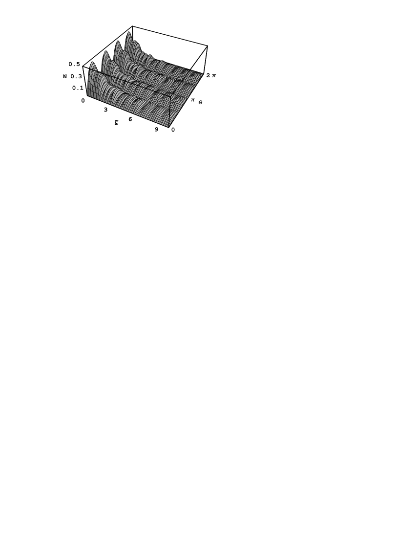
Figure 3: Surface plot of negativity as a function of Kerr medium $\zeta$ and phase angle $\theta$, when $T=1$, $\eta=1$, $n_{1}=n_{2}=100$.

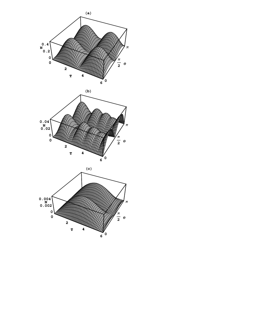
Figure 4: Surface plot of negativity as a function of time $T$ and phase angle $\theta$, when $\eta=1$, $\zeta=10$. (a) $n_{1}=n_{2}=0$; (b) $n_{1}=n_{2}=100$; (c) $n_{1}=0$, $n_{2}=100$.