Extension of the LTP temperature diagnostics to the LISA band: first results

Abstract

High-resolution temperature measurements are required in the LTP, i.e., 10 $\mu{\rm K}\,{\rm Hz}^{-1/2}$ from 1 mHz to 30 mHz. This has been already accomplished with thermistors and a suitable low noise electronics. However, the frequency range of interest for LISA goes down to 0.1 mHz. Investigations on the performance of temperature sensors and the associated electronics at frequencies around 0.1 mHz have been performed. Theoretical limits of the temperature measurement system and the practical on-ground limitations to test them are shown demonstrating that $1/f$ noise is not observed in thermistors even at frequencies around 0.1 mHz and amplitude levels of 10 $\mu$K Hz^-1/2.

Keywords: LISA, LISA Pathfinder, gravity wave detector, diagnostics, temperature measurements.

1 Introduction

The figure of merit of LISA related with its capability of detecting gravitational waves is the differential acceleration noise between the test masses of the satellites. This acceleration noise has been set to [1]

$$S_{\delta a,{\rm LISA}}^{1/2}(\omega)\leq 3\times 10^{-15}\,\left\{\left[1+\left(\frac{\omega/2\pi}{8\ {\rm mHz}}\right)^{\!\!4}\right]\!\left[1+\left(\frac{0.1\ {\rm mHz}}{\omega/2\pi}\right)\right]\right\}^{\!\frac{1}{2}}\ {\rm m}\,{\rm s}^{-2}\,{\rm Hz}^{-1/2}$$ (1)

in the frequency band between 0.1 mHz and 0.1 Hz.

LISA Pathfinder (LPF) is the pre-LISA mission in charge of demonstrating the capability of putting two test masses in free-fall at the levels needed for LISA. However, the LPF acceleration noise budget is reduced by one order of magnitude, both in amplitude and in frequency band [2], i.e.

$$S_{\delta a,{\rm LPF}}^{1/2}(\omega)\leq 3\!\times\!10^{-14}\,\left[1+\left(\frac{\omega/2\pi}{3\ {\rm mHz}}\right)^{\!\!2}\right]\,{\rm m}\,{\rm s}^{-2}\,{\rm Hz}^{-1/2}$$ (2)

for 1 mHz$\leq\omega/2\pi\leq 30$ mHz.

This acceleration noise is the result of various disturbances which limit the performance of the experiment [3]. The reades is referred to Lobo’s contribution to this volume for an overview of these disturbances. One of the noise sources is temperature fluctuations which translate into acceleration noise in the test masses by different mechanisms [4]. Those affecting directly the test masses are: (i) radiation pressure, (ii) radiometer effect and (iii) asymmetric outgassing; and the mechanisms disturbing the acceleration measurement, i.e., the interferometric subsystem are: (iv) temperature dependence of the index of refraction of optical components and (v) optical path length variations due to dilatation provoked by temperature changes [5]. This demands that temperature be monitored at different spots of the LTP. The main reasons are:

• to obtain information on the thermal behaviour of the LTP,

• to identify the fraction of noise in the test masses due to thermal effects,

• to validate whether or not the theoretical models related to thermal effects are accurate.

The role of the temperature diagnostics in LISA is still to be consolidated but, in principle, it will work at least as a noise cleaning tool, which will provide house-keeping data and will help to gravitational wave signal extraction.

The requirements for the temperature fluctuations in the LTP and LISA are [4]

$$S^{1/2}_{T,\ LTP}(\omega) \leq 100\,\mu{\rm K}\,{\rm Hz}^{-1/2},\hskip 8.5359pt1\,{\rm mHz}\leq\omega/2\pi\leq 30\,{\rm mHz}$$ (3)

$$S^{1/2}_{T,\ LISA}(\omega) \leq 10\,\mu{\rm K}\,{\rm Hz}^{-1/2},\hskip 8.5359pt0.1\,{\rm mHz}\leq\omega/2\pi\leq 100\,{\rm mHz}$$ (4)

The temperature measurement system (TMS) must be capable of measuring the expected temperature fluctuations within certain accuracy, for this reason the Noise Equivalent Temperature (NET) must be about one order of magnitude lower than the expected fluctuations [6], i.e.:

$$S^{1/2}_{T,\ LTP\ {\rm meas}}(\omega) \leq 10\,\mu{\rm K}\,{\rm Hz}^{-1/2},\hskip 8.5359pt1\,{\rm mHz}\leq\omega/2\pi\leq 30\,{\rm mHz}$$ (5)

$$S^{1/2}_{T,\ LISA\ {\rm meas}}(\omega) \leq 1\,\mu{\rm K}\,{\rm Hz}^{-1/2},\hskip 8.5359pt0.1\,{\rm mHz}\leq\omega/2\pi\leq 100\,{\rm mHz}$$ (6)

The TMS of the LTP has been already successfully tested and integrated in the Data Management Unit (DMU) of the LTP. Once we know the TMS is compliant with the requirements of the LTP [6, 7], the next natural step is to investigate the performance of the system at lower frequencies, i.e., extend the TMS of the LTP to the LISA band.

This article describes the noise investigations in the TMS of the LTP. The goal of this investigation is to detect whether or not the TMS designed for the LTP exhibits $1/f$ noise at frequencies lower than 1 mHz, specifically at frequencies around 0.1 mHz (LISA lowest frequency of interest). It is organised as follows: in section 2 a brief review of the results obtained with the TMS regarding the LTP requirements is shown. Section 3 details the problems related with the tests to assess the TMS performance in the LISA measurement bandwidth (MBW). Section 4 describes the active/passive temperature control designed to carry out successful tests at 0.1 mHz, and section 5 shows the results and conclusions from the experiments.

2 TMS requirement assessment for the LTP

The TMS implemented in the DMU of the LTP consists of a Negative Temperature Coefficient (NTC) thermistor (BetaTherm of nominal resistance 10 k$\Omega$) followed by a low-noise signal processing, fully detailed in [6]. The requirement of such system for the LTP is 10 $\mu{\rm K}\,{\rm Hz}^{-1/2}$ for $\omega/2\pi\geq 1$ mHz. In order to assess whether or not the system is compliant with the requirement we need to place the thermistors in a thermal environment more stable than the required NET, i.e., we must screen out laboratory temperature fluctuations to measure only the noise of the system. This implies the need to construct an insulator able to shield ambient temperature fluctuations about 5 orders of magnitude in the mili-hertz range. The concept of the insulator and the results obtained for a test campaign are shown in figure 1 where it is shown that the requirements for the LTP are fulfilled [4, 6].

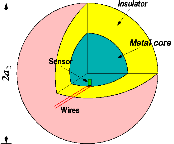
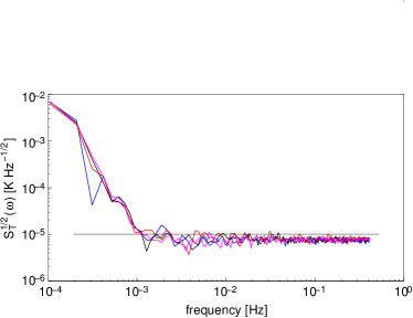
Figure 1: Left: Thermal insulator concept. A block of aluminium (0.2 m diameter) is surrounded by a polyurethane foam layer (0.6 m diameter). The attenuation of this jig at 1 mHz is enough to shield the ambient temperature fluctuations at the micro-Kelvin level. Right: Results from the LTP TMS flight model tests validation.

3 Extension to the LISA bandwidth: 0.1 mHz

Once the requirements for the LTP have been accomplished the next question, with an eye on LISA, is: do we have the same noise levels at 0.1 mHz? In principle, the electronic noise of the TMS should remain flat for all the frequencies due to the measurement method used [6], however, unexpected excess noise might appear at very low frequencies (0.1 mHz), specially, due to the semiconductor nature of the temperature sensor itself [8].

The tests in the submili-hertz region are considerably more complicated than the tests performed for the mili-hertz range. At frequencies down to 0.1 mHz the ambient temperature fluctuations become much larger and, in turn, the passive insulator attenuation appears to be quite poor, unless a prohibitively large insulator is built. The nominal ambient temperature fluctuations in the laboratory and the required temperature fluctuations inside the insulator are

$$S^{1/2}_{T,\ {\rm amb}}(0.1\,{\rm mHz}) \approx 1\ {\rm to}\ 10\ {\rm K}\,{\rm Hz}^{-1/2}$$ (7)

$$S^{1/2}_{T,\ {\rm ins}}(0.1\,{\rm mHz}) \approx 10\ \mu{\rm K}\,{\rm Hz}^{-1/2}$$ (8)

From equations (7) and (8) the needed attenuation at 0.1 mHz is readily calculated

$$|H_{\rm ins}(0.1{\rm mHz})|\leq 10^{-5}\ {\rm to}\ 10^{-6}$$ (9)

In order to obtain such an attenuation the needed passive insulator would consist in a aluminium sphere of 0.4 m diameter surrounded by a 2 m diameter polyurethane foam layer. However, the most discouraging reason to discard using a passive insulator is its time constant which is about 10 days. In consequence, temperature stabilisation down to 10 $\mu{\rm K}\,{\rm Hz}^{-1/2}$ at 0.1 mHz by using a mere passive insulator appears unreasonable.

3.1 Solution: differential measurements

A straight forward solution to avoid the need of a giant insulator is the use of differential temperature measurements instead of absolute temperature measurements. For the differential measurements we have that

$$S_{T_{1}}(\omega)=|H_{\rm ins}(\omega)|^{2}S_{T,{\rm amb}}(\omega)+n_{T_{1}}(\omega)$$ (10)

$$S_{T_{2}}(\omega)=|H_{\rm ins}(\omega)|^{2}S_{T,{\rm amb}}(\omega)+n_{T_{2}}(\omega)$$ (11)

where $n_{T_{1}}$ and $n_{T_{2}}$ are the noise of each of the thermistors plus electronic noise. Thus, the differential measurement fluctuations are

$$S_{\Delta T}(\omega)=n_{T_{1}}(\omega)+n_{T_{2}}(\omega)$$ (12)

Ideally, when differential measurements are made, only noise from the thermistors and the electronics is measured, since the common temperature fluctuations cancel out. Therefore, a very simple passive insulator would be enough. However, different non-idealities arise in the practical implementation which are discussed in the next section. Finally, we must keep in mind that the main concern about the potential $1/f$ noise in the submili-hertz range comes from the NTC thermistors which can be detected despite the differential measurements since we assume the $1/f$ noise of both thermistors is uncorrelated.

3.2 Real world limitations

Different non-idealities impede the straightforward tests of the TMS at very low frequency proposed in the previous section. The main limitations in the measurement that need to be overcome are:

• temperature coefficient (TC) of the electronics ($K_{FEE}$),

• cables connecting the thermistors to the electronics ($K_{\rm C}$),

• intrinsic differences between thermistors ($K_{NTC}$).

All these effects couple into the measurement and disturb the $1/f$ noise investigations. The apportioning of the these effects appears in the differential temperature measurements as (we have omitted the frequency dependent argument in the notation for simplicity)

$$S_{\Delta T}\approx n_{T_{1}}+n_{T_{2}}+K^{2}_{FEE}S_{T,\,{FEE}}+K^{2}_{\rm C}S_{T,\,{\rm amb}}+K^{2}_{NTC}S_{T,\,{\rm ins}}$$ (13)

where $S_{T,\,FEE}$, $S_{T,\ {\rm amb}}$ and $S_{T,\ {\rm ins}}$ stand for the temperature fluctuations in the electronics, in the laboratory and inside the insulator, respectively. The main objective is to determine $n_{T_{1}}+n_{T_{2}}$, hence, all the other contributions must be minimised. More specifically, we assign $\approx 5\mu{\rm K}\,{\rm Hz}^{-1/2}$ for each of the three disturbing terms.

The following sections detail these non-idealities and the solution adopted to overcome them.

3.2.1 Electronics temperature coefficient

The TC of the electronics implies that its temperature fluctuations appear in the temperature read-out as a fake temperature [6], i.e.,

$$S_{\Delta T}(\omega)=K^{2}_{FEE}S_{T,{FEE}}(\omega)$$ (14)

To determine the TC a high-stability resistor instead of a thermistor was connected to the FEE. The FEE was thermally excited by using a heater in order to estimate the TC when measuring the high-stability resistor. A scheme of the test set-up and the obtained measurements are shown in figure 2.

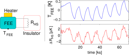
Figure 2: Left: test set-up scheme for the TC determination. One heater is used to excite thermally the FEE while its temperature and a high-stability resistor are measured. Top right: measured temperature of the FEE. Bottom right: high-stability resistance measurements in equivalent temperature.

From the measurements shown in figure 2 (right) the estimation of the parameter $K_{FEE}$ can be easily done. The value obtained is

$$\widehat{K}_{FEE}=13.5\ \mu{\rm K}/{\rm K}$$ (15)

This implies that in order to keep the effect of the TC below 5 $\mu$K Hz^-1/2 the FEE temperature fluctuations must be lower than 0.35 K Hz^-1/2 within the MBW which, in turn, means that the FEE must be thermostated since the ambient temperature fluctuations are around 1 K Hz^-1/2 at the 0.1 mHz range. The solution to this problem was solved by controlling the FEE temperature by means of a feedback control —see figure 7 (right).

3.2.2 Cables connecting thermistors to the FEE

Cables are a fair way for the ambient temperature fluctuations to appear in the thermistors’ measurements [4, 6]. Theoretically, differential measurements should fully reject the common mode ambient temperature, however, this is not the case due to mismatching between the cables and thermal resistance of both thermistors. This can be expressed as follows

$$S_{\Delta T}(\omega)=|H_{1}(\omega)-H_{2}(\omega)|^{2}S_{T,\ {\rm amb}}(\omega)$$ (16)

where $H_{1}$ and $H_{2}$ are the transfer functions relating the ambient temperature fluctuations to the thermistors’ ones. An estimation of $H_{1}-H_{2}$ was obtained by modeling the cables and the thermal contacts using a electrical analogy [9] —see figure 3.

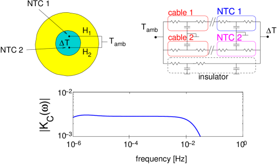
Figure 3: Common mode ambient temperature is not fully rejected due to mismatching between $H_{1}$ and $H_{2}$. These transfer functions include cables and thermal contact properties. Left: Lumped model for the $H_{1}-H_{2}$ transfer function. Right: $H_{1}-H_{2}$ transfer function. Cables are assumed identical for both sensors ($\ell$=0.25 m and 24 AWG) and thermal resistance are (measured): 95 K W^-1 and 100 K W^-1 for each of the thermistors.

The rejection of the ambient temperature is $\approx 3\times 10^{-3}$ at the frequencies of interest. This means that if ambient temperature fluctuations are about 1 K Hz^-1/2 at 0.1 mHz, the differential temperature measurement can result in about 3 mK Hz^-1/2, which is unacceptable considering that $\approx$5 $\mu$K Hz^-1/2 is the budgeted fluctuation for this effect. The solution adopted to reduce the common mode leakage is shown in figure 4 and consists of [10]:

• use of very thin cables (AWG32 instead of AWG24),

• use of longer cables (from $\ell$=0.25 m to $\ell$=2 m),

• attach cables to the aluminium block in order to dissipate the ambient temperature fluctuations prior to reach the thermistors: thermal trap.

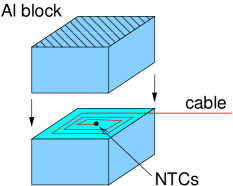
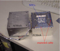
Figure 4: Left: Thermal trap concept. The ambient temperature fluctuations are attenuated in the aluminium block prior to reach the sensing head of the thermistor. Right: Physical implementation.

3.2.3 Intrinsic differences between thermistors

Once the problem of the leakage from the ambient temperature is solved, there is still another non-ideality: the inherent mismatch between each individual thermistor, i.e., even when two thermistor are measuring the same temperature, the differential temperature read-out is not zero due to differences in the response of each thermistor. The apportioning of this effect into the differential measurement is:

$$S_{\Delta T}(\omega)=|H_{1}(\omega)-H_{2}(\omega)|^{2}S_{T,\ {\rm ins}}(\omega)$$ (17)

where here $H_{1}-H_{2}$ is

$$H_{1}(\omega)-H_{2}(\omega)=\frac{q_{1}}{\sinh{aq_{1}}}-\frac{q_{2}}{\sinh{aq_{2}}}$$ (18)

with $a$ the radius of the NTC and

$$q_{j}=\frac{\rho_{j}c_{j}}{\kappa_{j}}i\omega$$ (19)

where $\rho_{j}$, $c_{j}$ and $\kappa_{j}$ are the density, the specific heat and the conductivity of the thermistors and their encapsulations, respectively. Equation (18) is difficult to evaluate due to the non-accurately known characteristics of the thermistors. However, it can be seen that equation (18) is, actually, a high-pass filter, i.e.

$$H_{1}(\omega)-H_{2}(\omega)\approx k_{NTC}i\omega$$ (20)

Experiments to estimate $k_{NTC}$ consisted of exciting thermally the aluminium block and measuring the absolute and the differential temperature. Figure 5 (left) shows the measurements that lead to the estimation of $\widehat{k}_{NTC}$=6 s. This effect implies that the temperature fluctuations of the insulator, $S_{T,{\rm ins}}$, must be limited to $\approx 5$ mK Hz^-1/2 at 0.1 mHz —see figure 5 (right)— which is not feasible for a passive insulator. In consequence, an active temperature controller together with the passive insulator —see section  4— was needed.

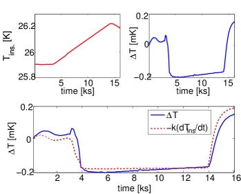
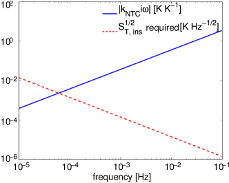
Figure 5: Left panel: the two top measurements correspond to the absolute temperature of the aluminium block (left) and the differential temperature measurement (right). The bottom plot shows the differential temperature measurement (solid trace) and the fitted one by derivation of the absolute temperature and adjusting the parameter to $k_{NTC}$=6 s (dashed trace). Right: solid trace is the transfer function relating absolute and differential temperature measurements. The dashed trace stands for the required temperature stability of the aluminium block to not disturb the tests.

4 Active/passive temperature controller

In order to keep the temperature fluctuations of the insulator at the required levels, a passive insulator plus an active temperature control based on a feedback-feedforward (FB-FF) scheme have been used. The former attenuates the temperature fluctuations above the mili-hertz region while the latter is useful to shield ambient temperature fluctuations at the submili-hertz region. Since the ambient temperature can be measured, the FB-FF control system can be implemented if good knowledge of the transfer functions involved in the control is provided [11]. The control system works as follows: a reference temperature for the aluminium block, $T_{\rm ref}$ (a few degrees over the ambient temperature), is set; then the control tries to maintain this temperature by dissipating power through a heater attached to the aluminium block. The applied power dissipated is calculated by a computer using the data coming from the ambient temperature (feedforward) and from the aluminium block temperature (feedback). The needed power is converted into a voltage which is supplied by a programmable power supply to the heater. The block diagram of the control system is given in figure 6 and its implementation scheme is shown in figure 7 (right).

Figure 6: Feedback-feedforward control temperature system block diagram. See text for details.

The closed-loop response is (in the $s$-domain, we omit the $s$ dependence argument in the rest of the paper for notation simplicity)

$$T_{\rm ins} = \frac{G_{\rm C}G_{\rm P}}{1+G_{\rm C}G_{\rm P}}T_{\rm ref}+\frac{H_{\rm ins}-G_{\rm C}G_{\rm P}G_{\rm F}}{1+G_{\rm C}G_{\rm P}}T_{\rm amb}+$$ (21)

$$+\frac{G_{\rm P}}{1+G_{\rm C}G_{\rm P}}n_{\rm act}+\frac{G_{\rm C}G_{\rm P}}{1+G_{\rm C}G_{\rm P}}n_{\rm sens}$$

where:

• $G_{\rm P}$ is the heater transfer function, i.e., the transfer function that relates the power dissipated in the heater and the increase of the temperature of the aluminium block,

• $H_{\rm ins}$ is the passive insulator transfer function, i.e., the attenuation of the ambient temperature fluctuations provided by the passive insulator,

• $G_{\rm C}$ is the controller transfer function, in our case a mere constant,

• $G_{\rm F}$ is the feedforward filter. In order to null the term multiplying the ambient temperature in equation (21) this filter must be

  $$G_{\rm F}=\frac{1}{G_{\rm C}}\frac{H_{\rm ins}}{G_{\rm P}}$$ (22)

  where all the transfer functions in the rhs of the equation are known. This filter is implemented digitally as a 11th order filter,

• $T_{\rm ref}$, $T_{\rm ins}$ and $T_{\rm amb}$ are the set point temperature for the aluminium block, the measured temperature of the aluminium block and the laboratory temperature, respectively,

• $n_{\rm act}$ and $n_{\rm sens}$ are the noise introduced by the programmable power supply and the noise of the absolute temperature sensor. Both are low enough not to disturb the test purposes.

Our main concern is to screen the ambient temperature fluctuations down to $\approx$5 mK Hz^-1/2 at 0.1 mHz —see figure 5 (right, dashed trace). In consequence, the figure of merit of the control loop is the transfer function relating the ambient temperature and the aluminium block temperature, i.e.,

$$T_{\rm ins}=\frac{H_{\rm ins}-G_{\rm C}G_{\rm P}G_{\rm F}}{1+G_{\rm C}G_{\rm P}}T_{\rm amb}$$ (23)

This transfer function is plotted in figure 7 (left) for different values of $G_{\rm C}$ where we realise that a value of $\approx 30$ is needed for $G_{\rm C}$ in order to obtain the required attenuation at the submili-hertz region (higher gains lead to an oscillating temperature response). Ideally, the solid traces in figure 7 (left) should all be zero, however, the digital implementation of the feedforward filter is only an approximation of the desired one, therefore, the differences between the approximated and the desired filter lead to a non-zero numerator in equation (23).

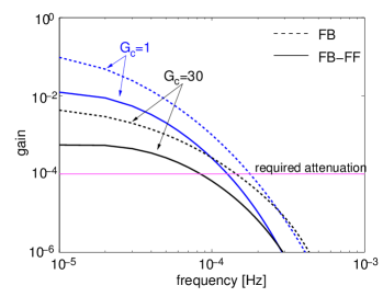
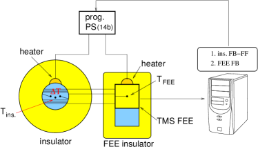
Figure 7: Left: Ambient temperature fluctuations screening. Solid traces represent the FB-FF for different gains, and dashed traces are plotted for comparison when using a FB scheme. Right: Control system implementation scheme. $G_{\rm C}$ was set to 30.

5 Results and conclusions

The results obtained are shown in figure 8. The solid trace labeled as “$\Delta T$” is the one standing for the differential measurement noise levels which does not exhibit any $1/f$ noise at the level of $\approx 10$ $\mu$K Hz^-1/2 down to 0.1 mHz. We can ascribe all this noise to the TMS itself (thermistors and electronics) since the required temperature fluctuations of the aluminium block (“$T_{\rm ins}$” trace) and the FEE temperature fluctuations (“$T_{FEE}$” trace) are within the required not to affect the measurement. We have added an extra measurement (trace at the bottom of the plot) which stands for the floor noise of the TMS when channels are not multiplexed. The noise of the TMS increases when measuring more than one channel due to the aliasing by a factor $\sqrt{N}$, with $N$ the numbers of channels [6]. The tests described here were performed acquiring 4 channels plus the control system. This implies lower sampling frequency which translates in extra noise in all the MBW due to aliasing.

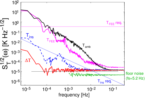
Figure 8: Tests results. “$T_{\rm amb}$” trace: ambient temperature fluctuations. “$T_{FEE}$” trace stands for the temperature fluctuations of the FEE while the “$T_{FEE}$ req.” trace represents its required stability. “$T_{\rm ins}$” trace stands for the aluminium temperature fluctuations, the “$T_{\rm ins}$ req.“ trace represents its required stability. ”$\Delta T$“ trace: differential measurement temperature fluctuations where we realise that exceed noise is not present down to 0.1 mHz. ”floor noise“ trace: independent measurement when acquiring only one channel. The rest of measurements were done acquiring 4 channels.

The conclusions of the noise investigations can be summarised:

• $1/f$ noise is not present in the thermistors and the associated electronics designed for the LTP, i.e., the noise remains flat down to 0.1 mHz with an amplitude level of $\approx 10$ $\mu$K Hz^-1/2,

• the floor noise when measuring a single channel goes down to $\approx$4 $\mu$K Hz^-1/2, at least, in the mili-hertz region,

• noise can be still further reduced by slight modifications in the electronics to reach noise levels close to 1 $\mu$K Hz^-1/2.

The above points mean that the thermal environment of the LTP can be measured with a limiting noise of $\approx$10 $\mu$K Hz^-1/2 down to 0.1 mHz. In views of LISA, the TMS can be slightly modified to reduce the NET to the $\mu$K Hz^-1/2 level.

References

References

- [1] The LISA International Science Team 2008 ESA-NASA, report no. LISA-ScRD-Iss5-Rev1
- [2] Vitale S 2005 Science Requirements and Top-level Architecture Definition for the LISA Technology Package (LTP) on Board LISA Pathfinder (SMART-2), report no. LTPA-UTN-ScRD-Iss003-Rev1
- [3] Araújo H et al 2007 Journal of Physics: Conference Series 66 012003
- [4] Lobo A, Nofrarias M, Ramos-Castro J and Sanjuán J 2006 Class Quantum Grav 23 5177
- [5] Nofrarias M et al 2007 Class Quantum Grav 24 5103
- [6] Sanjuán J, Lobo A, Nofrarias M, Ramos-Castro J and Riu P 2007 Rev Sci Instr 78 104904
- [7] Sanjuán J 2008 Noise performance TR for the FM Thermal Diagnostic Subsystem, report no. S2-IEEC-TR-3068
- [8] Pallàs R and Webster JG 2000 Sensors and signal conditioning (New York)
- [9] Incropera FP and DeWitt DP 1990 Fundamentals of heat and mass transfer (New York)
- [10] Dratler J 1974 Rev Sci Instr 45 1435
- [11] Phillips CL, Royce DH 1996 Feedback control systems (New Jersey)