Ageing in bosonic particle-reaction models with long-range transport

Xavier Durang and Malte Henkel

Département de Physique de la Matière et des Matériaux,

Institut Jean Lamour, CNRS – Nancy Université – UPVM,

B.P. 70239, F – 54506 Vandœuvre lès Nancy Cedex, France

Ageing in systems without detailed balance is studied in bosonic contact and pair-contact processes with Lévy diffusion. In the ageing regime, the dynamical scaling of the two-time correlation function and two-time response function is found and analysed. Exact results for non-equilibrium exponents and scaling functions are derived. The behaviour of the fluctuation-dissipation ratio is analysed. A passage time from the quasi-stationary regime to the ageing regime is defined, in qualitative agreement with kinetic spherical models and $p$-spin spherical glasses.

PACS: 05.20.-y, 05.40.Fb, 64.60.Ht, 64.70.qj

1 Introduction

One of the paradigmatic example of non-equilibrium critical behaviour is furnished by ageing systems. A common way to realise physical ageing is to move a system rapidly out of equilibrium by ‘quenching’ some thermodynamic parameter into a coexistence region of its phase diagramme such that there exist several competing thermodynamical states. Alternatively, one may quench a system exactly onto a critical point of its stationary state, which is the case we shall study in this paper. From a phenomenological point of view, physical ageing may by characterised by the three properties of (i) slow, i.e. non-exponential dynamics, (ii) breaking of time-translation-invariance and (iii) dynamical scaling.

Although physical ageing was first recognised and studied in glassy systems, starting from Struik’s classical experiments [44, 45], the analysis of many aspects of ageing is more simple in non-glassy systems without disorder or frustrations. Typical examples of this kind are simple ferromagnets, the dynamics of which can be characterised in terms of a single time-dependent length scale $L(t)\sim t^{1/z}$, which defines the dynamic exponent, see [11, 12] for reviews. Their ageing behaviour is conveniently studied through the two-time correlation and response functions of the time-dependent order-parameter $\phi(t)$, for which ones expects the scaling behaviour

$$C(t,s) = \langle\phi(t)\phi(s)\rangle-\langle\phi(t)\rangle\langle\phi(s)\rangle\>=\>s^{-b}f_{C}(t/s)$$ (1.1)

$$R(t,s) = \left.\frac{\delta\langle\phi(t)\rangle}{\delta h(s)}\right|_{h=0}\>=\>s^{-1-a}f_{R}(t/s)$$ (1.2)

where $h(s)$ is an external magnetic field conjugate to the order-parameter, and $t,s$ are the observation and waiting times, respectively. This scaling behaviour should be valid in the ageing regime $t,s\gg\tau_{micro}$ and $t-s\gg\tau_{micro}$ where $\tau_{micro}$ is a microscopic reference time. From the asymptotic behaviour $f_{C,R}(y)\sim y^{-\lambda_{C,R}/z}$ of the scaling functions as $y\to\infty$ one may define the autocorrelation and autoresponse exponents $\lambda_{C}$ and $\lambda_{R}$, respectively. The exponents $a,b$ are known as ageing exponents and can be expressed in terms of $z$ and static critical exponents. For reviews, see e.g. [11, 14, 21, 12, 25].

In this paper, we are interested in systems where the underlying dynamics does not satisfy detailed balance such that the stationary state is no longer an equilibrium state. Recently, it was shown that the same kind of non-equilibrium scaling behaviour (1.1,1.2) as described above for ageing ferromagnets applies to this kind of systems, as exemplified for the critical contact process [19, 41, 8] and the critical non-equilibrium kinetic Ising model [36]. However, in contrast to the non-equilibrium critical dynamics of ferromagnets, the ageing exponents $a$ and $b$ need no longer to be equal, which for the contact process can be understood as a consequence of its model-specific rapidity-reversal-symmetry [8]. Furthermore, there are exactly solvable models such as the so-called ‘bosonic’ contact and pair-contact processes [28, 37, 38] for which the ageing behaviour could be analysed in full detail and the non-equilibrium exponents and scaling functions be calculated exactly [5]. The critical behaviour of the ‘bosonic’ models is different from the more usually studied ‘fermionic’ ones since, although the average total number of particles is conserved at criticality, for long times the particles may condense onto a single site which mimics the inhomogeneous growth of bacteria colonies and had originally led to the formulation of the BCPD [46, 28] and BPCPD. All these models show ageing only when brought to the critical point(s) of the stationary states, see [24] for a recent review. They also have in common that transport of single particles is only through the ‘diffusive’ hopping to nearest-neighbour sites. We wish to investigate the consequences when that local, nearest neighbour transport of single particles is replaced by long-range Lévy flights, leading to superdiffusive behaviour. There are several motivations for such an undertaking:

1. Lévy flights [43, 35] generalise the usually considered local (brownian) random walks in that they lead to a generalised central limit theorem for the sum of a large number of independent random variables. Heuristically, it appears reasonable to consider the ‘particles’ which make up the basic dynamics of non-equilibrium systems as coarse-grained variables which arise from summing over many more microscopic degrees of freedom. It may hence appear natural that the effects of long-range jumps between distant sites should be taken into consideration. This might become relevant for the description of traces particles in turbulent flows or the spreading of epidemics, see [34] and refs there in.

2. When studying the ordinary contact process with Lévy flights, it has been shown that the critical behaviour of the stationary state, as well as the relaxation behaviour, is modified [27, 31, 16, 2, 26].

The models under study are defined as follows. Each site of an infinite $d$-dimensional hyper-cubic lattice may contain an arbitrary positive number of particles. Particles on the same site can undergo the reactions

$$mA \longrightarrow (m+k)A\hskip 56.9055pt\mbox{\rm with rate $\mu$}$$

$$mA \longrightarrow (m-\ell)A\hskip 56.9055pt\mbox{\rm with rate $\lambda$}$$ (1.3)

Furthermore, single particles can hop to another site at distance $|\boldsymbol{r}|$, with a rate

$$D({\mathbb{r}})=\frac{D}{(2\pi)^{d}}\int_{-\infty}^{\infty}\!{\rm d}^{d}{\mathbb{q}}\>e^{\left({\rm i}{\mathbb{q}}\cdot{\mathbb{r}}-c\|{\mathbb{q}}\|^{\eta}\right)}$$ (1.4)

where $0<\eta<2$ is a control parameter and $c$ is a non-universal dimensionful constant. The case $m=1$ (and with $k=\ell=1$) is called the bosonic contact process with Lévy flight (BCPL) and the case $m=2$ is called the bosonic pair-contact process with Lévy flight (BPCPL).

In section 2, we write down the closed set of equations of motion for the correlation and response functions. In section 3, we discuss the phase diagram, exponents and scaling functions for both models. In section 4, we verify that the exact scaling functions found for the bosonic contact process can be understood from the theory of local scale-invariance. A discussion of local scale-invariance for bosonic pair-contact process with Lévy diffusion will be presented in a sequel paper. In section 5, we study the passage from the quasi-stationary regime to the ageing regime and identify the passage exponent $\zeta$ which characterises the relevant time-scale $\tau_{p}(s)\sim s^{\zeta}$ [47], for the first time in a critical system. In section 6, we present our conclusions. Finally, we derive in appendix A a relation for the physical interpretation of the two-time correlators, list in appendix B the scaling functions for the space-time correlators and responses and present in appendix C the analysis of the passage time in the critical spherical model.

2 Equations of motion

Following [37], the master equation is written in the quantum hamiltonian/Liouvillian formulation (for reviews, see [42, 26]) as $\partial_{t}|P(t)\rangle=-H|P(t)\rangle$ where $P(t)$ is the time-dependent state vector and the hamiltonian can be expressed in terms of annihilation and creation operators $a({\mathbb{x}})$ and $a^{\dagger}({\mathbb{x}})$. We also define the particle number operator as $n({\mathbb{x}})=a^{\dagger}({\mathbb{x}})a({\mathbb{x}})$. The Hamiltonian reads

$$\begin{split}H=&-\sum_{{\mathbb{r}}\neq{\mathbb{0}}}\sum_{{\mathbb{x}}}D({\mathbb{r}})[a({\mathbb{x}})a^{\dagger}({\mathbb{x}}+{\mathbb{r}})-n({\mathbb{x}})]\\ &-\lambda\sum_{{\mathbb{x}}}[a^{\dagger}({\mathbb{x}})^{m-\ell}a({\mathbb{x}})^{m}-\prod_{i=1}^{m}(n({\mathbb{x}})-i+1)]\\ &-\mu\sum_{{\mathbb{x}}}[a^{\dagger}({\mathbb{x}})^{m+k}a({\mathbb{x}})^{m}-\prod_{i=1}^{m}(n({\mathbb{x}})-i+1)]-\sum_{{\mathbb{x}}}h({\mathbb{x}})a^{\dagger}({\mathbb{x}})\end{split}$$ (2.1)

For the computation of the response function, we also added an external field which describes the spontaneous creation of a single particle with a site-dependent rate $h=h({\mathbb{x}})$ on the site ${\mathbb{x}}$.

Single-time observables $g(t,{\mathbb{x}})$ can be obtained from the time-independent quantities by switching to the Heisenberg picture. The differential equations for the desired quantities can be obtained by using the usual Heisenberg equation of motion $\partial_{t}g=\left[g,H\right]$. The space-time dependent particle density $\rho(t,{\mathbb{x}})=\langle a^{\dagger}(t,{\mathbb{x}})a(t,{\mathbb{x}})\rangle=\langle a(t,{\mathbb{x}})\rangle$ satisfies

$$\begin{split}\frac{\partial}{\partial t}\langle a(t,{\mathbb{x}})\rangle=&\sum_{{\mathbb{r}}\neq{\mathbb{0}}}D({\mathbb{r}})[\langle a(t,{\mathbb{x}}+{\mathbb{r}})\rangle-\langle a(t,{\mathbb{x}})\rangle]\\ &-\lambda\ell\langle a(t,{\mathbb{x}})^{m}\rangle+\mu k\langle a({t,\mathbb{x}})^{m}\rangle+h({t,\mathbb{x}})\end{split}$$ (2.2)

For the bosonic contact process BCPL, this equation closes for arbitrary values of the rates. However, for the bosonic pair-contact process BPCPL, we only find a closed set of equations along the critical line defined as

$$\sigma=\frac{\mu k-\lambda\ell}{D}\stackrel{{\scriptstyle!}}{{=}}0$$ (2.3)

As we shall see later, along the critical line the space-integrated particle density

$$\rho_{0}:=\int\!{\rm d}\boldsymbol{x}\>\rho(t,\boldsymbol{x})=\int\!{\rm d}\boldsymbol{x}\>\langle a(t,\boldsymbol{x})\rangle$$ (2.4)

is conserved, although the microscopic process can change the total number of particles in the system. All this is completely analogous to what was already known for the BCPD and BPCPD.

Throughout this paper, we are interested in the correlation and response functions

$$C(t;\boldsymbol{r}) = \langle a(t,\boldsymbol{x})a(t,\boldsymbol{x}+\boldsymbol{r})\rangle-\rho_{0}^{2}$$

$$C(t,s;\boldsymbol{r}) = \langle a(t,\boldsymbol{x})a(s,\boldsymbol{x}+\boldsymbol{r})\rangle-\rho_{0}^{2}$$ (2.5)

$$R(t,s;\boldsymbol{r}) = \left.\frac{\delta\langle a(t,\boldsymbol{x}+\boldsymbol{r})\rangle}{\delta h(s,\boldsymbol{x})}\right|_{h=0}$$

In these notations, we already anticipate spatial translation-invariance. The single-time correlator is determined from the following equations of motion

$$\begin{split}\frac{\partial}{\partial t}\langle a(t,{\mathbb{x}})a(t,{\mathbb{x}})\rangle=&\,2\sum_{{\mathbb{r}}\neq{\mathbb{0}}}D({\mathbb{r}})[\langle a({t,\mathbb{x}})a({t,\mathbb{x}}+{\mathbb{r}})\rangle-\langle a(t,{\mathbb{x}})^{2}\rangle]\\ &+\lambda\ell[(1+\ell-2m)\langle a(t,{\mathbb{x}})^{m}\rangle-2\langle a(t,{\mathbb{x}})^{m+1}\rangle]\\ &-\mu k[(1-k-2m)\langle a(t,{\mathbb{x}})^{m}\rangle-2\langle a(t,{\mathbb{x}})^{m+1}\rangle]\end{split}$$ (2.6)

and for ${\mathbb{x}}\neq{\mathbb{y}}$

$$\begin{split}\frac{\partial}{\partial t}\langle a(t,{\mathbb{x}})a(t,{\mathbb{y}})\rangle=&\sum_{{\mathbb{r}}\neq{\mathbb{0}}}D({\mathbb{r}})[\langle a(t,{\mathbb{x}})a(t,{\mathbb{y}}+{\mathbb{r}})\rangle+\langle a(t,{\mathbb{x}}+{\mathbb{r}})a(t,{\mathbb{y}})\rangle-\langle a(,t{\mathbb{x}})a(,t{\mathbb{y}})\rangle]\\ &-\lambda\ell[\langle a(t,{\mathbb{x}})a(t,{\mathbb{y}})^{m}\rangle-\langle a(t,{\mathbb{x}})^{m}a(t,{\mathbb{y}})\rangle]\\ \\ &+\mu k[\langle a(t,{\mathbb{x}})a(t,{\mathbb{y}})^{m}\rangle-\langle a(t,{\mathbb{x}})^{m}a(t,{\mathbb{y}})\rangle]\end{split}$$ (2.7)

In particular, these equations close along the critical line (2.3). The equation of motion of the two-time correlator reads

$$\begin{split}\frac{\partial}{\partial t}\langle a(t,{\mathbb{x}})a({s,\mathbb{y}})\rangle=&\sum_{{\mathbb{n}}\neq{\mathbb{0}}}D({\mathbb{n}})[\langle a(t,{\mathbb{x}}+{\mathbb{n}})a(s,{\mathbb{y}})\rangle-\langle a(t,{\mathbb{x}})a(s,{\mathbb{y}})\rangle]\\ &-\lambda\ell\langle a(t,{\mathbb{x}})^{m}a(s,{\mathbb{y}})\rangle+\mu k\langle a(t,{\mathbb{x}})^{m}a(s,{\mathbb{y}})\rangle\end{split}$$ (2.8)

together with the initial condition $\lim_{t\to s}\langle a(t,\boldsymbol{x})a(s,\boldsymbol{y})\rangle=\langle a(t,\boldsymbol{x})a(t,\boldsymbol{y})\rangle$.

The relationship of these correlators with the average density and its variance are given for diffusive transport by $\langle n(t,\boldsymbol{x})\rangle=\langle a(t,\boldsymbol{x})\rangle$ and $\langle n(t,\boldsymbol{x})^{2}\rangle=\langle a(t,\boldsymbol{x})^{2}\rangle+\langle a(t,\boldsymbol{x})\rangle$ [37] and more generally by [4], using also the definitions (2.5)

$$\langle n(t,\boldsymbol{x})n(s,\boldsymbol{x}+\boldsymbol{r})\rangle-\rho_{0}^{2}=C(t,s;\boldsymbol{r})+\rho_{0}R(t-s,\boldsymbol{r})$$ (2.9)

In appendix A, we generalise the proof of these relations to the case at hand. We shall show there that the second term in (2.9) is merely generating corrections to the leading scaling behaviour so that for our purposes, $C(t,s;\boldsymbol{r})$ can be interpreted as a connected density-density correlator.

We begin the analysis of the equations of motion with the particle-density. For the BCPL, as well as for the BPCPL with $\sigma=0$, one can Fourier-transform eq. (2.2), with the result

$$\frac{\partial}{\partial t}\langle\widetilde{a}(t,{\mathbb{q}})\rangle=-\frac{1}{2}\underbrace{\sum_{{\mathbb{n}}\neq{\mathbb{0}}}\frac{D({\mathbb{n}})}{D}(1-e^{i{\mathbb{q}}\cdot{\mathbb{n}}})}_{=:\,\omega(\boldsymbol{q})}\;\;\langle\widetilde{a}(t,{\mathbb{q}})\rangle+\frac{\sigma}{2}\langle\widetilde{a}(t,{\mathbb{q}})\rangle+\widetilde{h}(t,{\mathbb{q}})$$ (2.10)

which defines the dispersion relation $\omega(\boldsymbol{q})$. If we can perform a continuum limit

$$\omega({\mathbb{q}})=1-e^{-c\|{\mathbb{q}}\|^{\eta}}\underset{{\mathbb{q}}\rightarrow{\mathbb{0}}}{\approx}c\|{\mathbb{q}}\|^{\eta}$$ (2.11)

from which we read off the expected dynamical exponent $z=\eta$.

Similarly, we calculate the response function by applying its definition (2.5) to the equation of motion (2.2). This becomes in Fourier space (again, one must set $\sigma=0$ for the BPCPL)

$$\frac{\partial}{\partial t}\widetilde{R}(t,s;{\mathbb{q}})=-\frac{1}{2}\omega({\mathbb{q}})\widetilde{R}(t,s;{\mathbb{q}})+\frac{\sigma}{2}\widetilde{R}({t,s;\mathbb{q}})+\delta(t-s)$$ (2.12)

Consequently, the real-space response function reads

$$R({t,s;\mathbb{r}})=\frac{1}{(2\pi)^{d}}\underbrace{\int_{B}{\rm d}^{d}{\mathbb{q}}\>e^{i{\mathbb{q}}\cdot{\mathbb{r}}}\>e^{-\frac{1}{2}\omega({\mathbb{q}})(t-s)}}_{=:b({\frac{t-s}{2},\mathbb{r}})}\;\exp\left({\frac{\sigma(t-s)}{2}}\right)\Theta(t-s)$$ (2.13)

where $B$ is the Brillouin zone and the $\Theta$-function expresses causality. In particular, for long times the autoresponse becomes for $t>s$

$$R({t,s;\mathbb{0}})\simeq e^{\frac{\sigma}{2}(t-s)}\left(\frac{t-s}{2}\right)^{-d/\eta}\frac{1}{(2\pi)^{d}}\int_{0}^{\infty}{\rm d}^{d}{\mathbb{q}}\;e^{-\|{\mathbb{q}}\|^{\eta}c}=\frac{2^{1-d}}{\pi^{d/2}}\frac{\Gamma\left(d/\eta\right)}{\eta\Gamma\left(d/2\right)}e^{\frac{\sigma}{2}(t-s)}\left(c\frac{t-s}{2}\right)^{-d/\eta}$$ (2.14)

For the correlation function, we shall assume that spatial translation-invariance holds and use the non-connected correlator $F(t,s;\mathbb{r}):=\langle a(t,{\mathbb{x}})a(s,{\mathbb{x}}+{\mathbb{r}})\rangle$ and also introduce the control parameter

$$\alpha=\frac{\mu k(k+\ell)}{2D}$$ (2.15)

As initial conditions, we shall use throughout the Poissonian distribution $F(0,0;{\mathbb{r}})=\rho_{0}^{2}$. Generalising slightly the calculations performed earlier for the BCPD and BPCPD [37, 5], we find for the BCPL the connected correlation function (on the critical line $\sigma=0$)

$$C(t,s;{\mathbb{r}})=\alpha\rho_{0}\int_{0}^{s}{\rm d}\tau\>b(\frac{t+s}{2}-\tau,{\mathbb{r}})\simeq\alpha\rho_{0}\int_{0}^{s}{\rm d}\tau\>\int_{B}\frac{{\rm d}^{d}{\mathbb{q}}}{(2\pi)^{d}}\exp\left({-c\|{\mathbb{q}}\|^{\eta}\left(\frac{t+s}{2}-\tau\right)}-{\rm i}\boldsymbol{r}\cdot\boldsymbol{q}\right)$$ (2.16)

where the long-time limit $t,s\gg t_{\rm micro}$ and $t-s\gg t_{\rm micro}$ was also taken. See appendix B for the computational details. For the bosonic pair-contact process BPCPL, we first consider the non-connected single-time correlation function $F(t,\boldsymbol{r})$ which satisfies the equation

$$\begin{split}F(t,{\mathbb{r}})&=\rho_{0}^{2}+\alpha\int_{0}^{t}{\rm d}\tau\>F(\tau,{\mathbb{0}})\int_{B}\frac{{\rm d}^{d}{\mathbb{q}}}{(2\pi)^{d}}e^{-\omega({\mathbb{q}})\left(t-\tau\right)}e^{{\rm i}{\mathbb{q}}\cdot{\mathbb{r}}}\\ &=\rho_{0}^{2}+\alpha\int_{0}^{t}{\rm d}\tau\>F(\tau,{\mathbb{0}})\>b(t-\tau,{\mathbb{r}})\end{split}$$ (2.17)

For ${\mathbb{r}}=0$, this is a Volterra integral equation for $F({t,\mathbb{0}})$ which may be solved by Laplace transformation as in ([37], [5]). The $F(t,{\mathbb{r}})$ is then directly obtained from (2.17). Having found this, the two-time correlator is given by

$$F(t,s,\boldsymbol{r})=\rho_{0}^{2}+\alpha\int_{0}^{s}{\rm d}\tau F(\tau,\boldsymbol{0})b\left(\frac{t+s}{2}-\tau,\boldsymbol{r}\right)$$ (2.18)

The results of eqs. (2.16,2.17,2.18) will form the basis of the subsequent analysis. The essential difference with respect to the BCPD and BPCPD is the different form of the dispersion $\omega(\boldsymbol{q})$.

3 Exact solution

3.1 Phase diagramme

Since the total number of particles is conserved on average, information on the critical behaviour comes by analysing the variance $\langle n(t,\boldsymbol{r})^{2}\rangle$. The resulting phase diagramme is presented in figure 1. There are two distinct phases separated by the critical line eq. (2.3), namely (i) an absorbing phase for $\lambda>\mu$ with a vanishing particle-density in the steady-state, and (ii) an active phase for $\lambda<\mu$, where the particle-density diverges for large times. Along the critical line, the total mean particle-density is constant. The behaviour of the model along the critical line, described by varying the control parameter $\alpha$ eq. (2.15) is as follows:

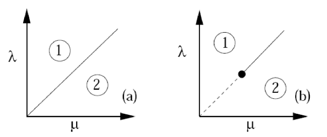
Figure 1: Schematic phase-diagrammes for $d\neq 0$ of (a) the BCPL and the BPCPL in $d\leq\eta$ and (b) the BPCPL in $d>\eta$. The absorbing region $1$ for $\lambda>\mu$, where the particle-density vanishes at large time, is separated by the critical line eq. (2.3) from an active region for $\lambda<\mu$, where the particle-density diverges at large times. Along the critical line, the average time-dependent particle-density remains constant.

• For the bosonic contact process BCPL, one has the same critical behaviour for all values of $\alpha$. On the other hand, the value of the space dimension $d$ is very important. If $d\leq\eta$, one has clustering: for long times, the particles are on average redistributed such as only a few, spontaneously selected, lattice sites contain particles while the others become essentially empty. For $d>\eta$, the long-time particle-density is spatially homogeneous.

  We can interpreted this result by using a generalised Polya theorem [39], which states that for $d<\eta$ the Lévy random walk is recurrent and hence cannot homogenise the system. On the other hand, when $d>\eta$, there is a non-zero probability that a Lévy random walk does not return to its starting point. This is enough to make the system spatially homogeneous.

• For the bosonic pair-contact process BPCPL, when $d<\eta$, there is always clustering. On the other hand, for $d>\eta$, there is a multi-critical point at $\alpha=\alpha_{C}$ such that the system is homogeneous for $\alpha<\alpha_{C}$ and that one has clustering for $\alpha>\alpha_{C}$. The critical point of this clustering transition is given by

  $$\alpha_{C}=\left(2\int_{B}\frac{{\rm d}^{d}\boldsymbol{q}}{(2\pi)^{d}}(2\omega(\boldsymbol{q}))^{-1}\right)^{-1}$$ (3.1)

  From this expression, one sees that $\alpha_{C}\to\infty$ if $d\to\eta$ [21, 6].

3.2 Ageing exponents and scaling functions

Using the explicit expressions from section 2, we can perform the long-time limit and by comparing with the scaling forms eqs. (1.1,1.2) we can proceed to extract the non-equilibrium critical exponents, which are listed in table 1 and then the scaling functions which, up to a normalisation factor, are given in table 2. For the details of the calculation, see appendix B.

	Bosonic	Bosonic pair-contact process
	contact process	$\alpha<\alpha_{C}$	$\alpha=\alpha_{C}$
$a$	$\frac{d}{\eta}-1$	$\frac{d}{\eta}-1$	$\frac{d}{\eta}-1$
$b$	$\frac{d}{\eta}-1$	$\frac{d}{\eta}-1$	$0$	if	$\eta<d<2\eta$
			$\frac{d}{\eta}-2$	if	$d>2\eta$
$\lambda_{R}$	$d$	$d$	$d$
$\lambda_{C}$	$d$	$d$	$d$
$z$	$\eta$	$\eta$	$\eta$

Table 1: Ageing exponents of the critical BCPL and BPCPL in different regimes. The results for the BCPL hold true for any dimension $d$, while for the BPCPL they only apply if $d>\eta$.

			$f_{R}(y)$	$f_{C}(y)$
Bosonic contact process			$(y-1)^{-d/\eta}$	$(y-1)^{-d/\eta+1}-(y+1)^{-d/\eta+1}$
Bosonic	$\alpha<\alpha_{C}$	$d>\eta$	$(y-1)^{-d/\eta}$	$(y-1)^{-d/\eta+1}-(y+1)^{-d/\eta+1}$
pair contact	$\alpha=\alpha_{C}$	$\eta<d<2\eta$	$(y-1)^{-d/\eta}$	$(y+1)^{-d/\eta}\;_{2}F_{1}\left(\frac{d}{\eta},\frac{d}{\eta};\frac{d}{\eta}+1;\frac{2}{y+1}\right)$
process		$d>2\eta$	$(y-1)^{-d/\eta}$	$2(d-2\eta)(y-1)^{1-d/\eta}$
				$-\eta(y-1)^{2-d/\eta}+\eta(y+1)^{2-d/\eta}$

Table 2: Scaling functions of the autoresponse and autocorrelation function of the critical bosonic contact and pair-contact processes. They are given up to a multiplicative factor.

Some comments are in order.

• If $d>\eta$ and if furthermore $\alpha<\alpha_{C}$ in the BPCPL, the anticipated dynamical scaling (1.1,1.2) holds true for both the BCPL and the BPCPL. Furthermore, since the exponents and the form of the scaling functions agree, the two models are in the same universality class.

• For $d<\eta$, we still find a dynamical scaling behaviour in the BCPL. We observe that the exponents $a=b$ now become negative. This reflects the eventual condensation of the particles which means that the fluctuations diverge for large times.

  For the BPCPL however, for $d<\eta$ or more generally $\alpha>\alpha_{C}$, no dynamical scaling is found. Rather, the variance diverges exponentially with time. The notion of ageing as defined in the introduction no longer applies here.

• Finally, for the BPCPL with $d>\eta$ and at the tricritical point $\alpha=\alpha_{C}$, the dynamical scaling (1.1,1.2) holds true. The values of the non-equilibrium exponents are distinct from those of the universality class discussed above and in particular, we note that $a\neq b$ although still $\lambda_{C}=\lambda_{R}$. In this respect, the absence of detailed balance has led in this case to an ageing behaviour intrinsically different from the non-equilibrium dynamics of a ferromagnet (where $a=b$ as well as $\lambda_{C}=\lambda_{R}$ always hold true).

• The response function $R=R(t-s;\boldsymbol{r})$ has a particularly simple form which actually obeys time-translation-invariance. However, since time-translation-invariance is not satisfied for the two-time correlators, the notion of ageing is still applicable.

If we identify the upper critical dimension as $d^{*}=\eta$, we see that our results can be mapped onto those [5] of the BCPD and BPCPD if one replaces $d/\eta=d/d^{*}\mapsto d/2$.

4 Local scale-invariance

We now inquire whether the forms of the scaling functions derived in the previous section can be understood from some larger dynamical symmetry than mere dynamical scaling.

Indeed, for simple ferromagnets undergoing phase-ordering kinetics after a quench from a totally disordered initial state to the ordered phase with a temperature $T<T_{c}$, an extension of dynamical scaling [11] to a local group of time-dependent scale-transformation related to a subgroup of the Schrödinger group (without time translations) has been found [23, 25]. In particular, it has been understood how to use the necessarily projective representations of non-semisimple groups as the Schrödinger group in order to analyse the dynamical symmetries of the stochastic Langevin equations underlying these phenomena [40]. The essential tool in this kind of analysis are the celebrated Bargmann superselection rules [3]. Then both response as well as correlation functions can be explicitly calculated and the results have been successfully tested in numerous models, see [25] for a review. Since the Schrödinger group and its subgroups only apply to physical situations where the dynamical exponent $z=2$, a generalisation to arbitrary values of $z$ must be sought.

4.1 Background

In this section, we shall use the BCPL with $z=\eta<2$ as an analytically treatable test case for such a possible extension. In order to do so, we shall first reformulate the problem as a non-equilibrium field-theory using the Janssen-de Dominicis theory [15, 30, 29]. Starting from the master equation with the reaction rates eqs. (1,1.4), the creation and annihilation operators become related in the continuum limit to the order-parameter field and a conjugate response field

$$\phi(t,{\mathbb{r}}) :=a(t,{\mathbb{r}})-\rho_{0}$$ (4.1)

$$\widetilde{\phi}(t,{\mathbb{r}}) :=a^{\dagger}(t,{\mathbb{r}})-1$$ (4.2)

such that $\langle\phi(t,{\mathbb{r}})\rangle=\langle\widetilde{\phi}(t,{\mathbb{r}})\rangle=0$. The action associated to the critical BCPL reads

$${\cal J}[\phi,\widetilde{\phi}]=\int\!{\rm d}{\mathbb{R}}\int\!{\rm d}u\;\left[\widetilde{\phi}(2{\cal M}\partial_{u}-\Delta^{\eta/2})\phi-\mu\widetilde{\phi}^{2}(\phi+\rho_{0})\right]={\cal J}_{0}[\phi,\widetilde{\phi}]+{\cal J}_{b}[\phi,\widetilde{\phi}]$$ (4.3)

where we have suppressed the arguments of $\phi(u,{\mathbb{R}})$ and $\widetilde{\phi}(u,{\mathbb{R}})$ under the integrals. The dimensionful ‘mass’ $\cal M$ is related to a generalised diffusion constant. The action is decomposed into two parts: a so-called ‘deterministic’ (noiseless) part

$${\cal J}_{0}[\phi,\widetilde{\phi}]=\int\!{\rm d}{\mathbb{R}}\int\!{\rm d}u\;\left[\widetilde{\phi}(2{\cal M}\partial_{u}-\Delta^{\eta/2})\phi\right]$$ (4.4)

and a ‘noise’ part

$${\cal J}_{b}[\phi,\widetilde{\phi}]=-\int\!{\rm d}{\mathbb{R}}\int\!{\rm d}u\;\left[\mu\widetilde{\phi}^{2}(\phi+\rho_{0})\right]$$ (4.5)

Here the non-integral power of the Laplacian has to be interpreted as a fractional derivative [4, 9]. In this formalism, correlators and response functions are found as follows:

$$C(t_{1},\ldots,t_{n};\boldsymbol{r}_{1},\ldots\boldsymbol{r}_{n}) = \langle\phi_{1}(t_{1},{\mathbb{r}}_{1})\ldots\phi_{n}(t_{n},{\mathbb{r}}_{n})\rangle$$

$$R(t,s;\boldsymbol{r},\boldsymbol{r}^{\prime}) = \langle\phi(t,{\mathbb{r}})\widetilde{\phi}(s,{\mathbb{r}}^{\prime})\rangle$$ (4.6)

where the average of any observable $A$ is given by the functional integral $\langle A\rangle=\int\!\mathcal{D}\phi\mathcal{D}\widetilde{\phi}\>A[\phi,\widetilde{\phi}]e^{-{\cal J}[\phi,\tilde{\phi}]}$. As we have shown earlier for the case $z=2$ [40], one considers first the ‘deterministic’ part of the action, obtained from the variation of ${\cal J}_{0}$ with respect to $\widetilde{\phi}$. The associated equation of motion

$${\cal S}\phi=\left(2{\cal M}\partial_{t}-\Delta^{\eta/2}\right)\phi=0$$ (4.7)

has a dynamical symmetry under the infinitesimal generators of local scale-transformations [4, 9]

$$X_{-1}:=-\partial_{t}$$ time-translation

$$X_{0}:=-t\partial_{t}-\frac{1}{\eta}(\boldsymbol{r}\cdot\partial_{\boldsymbol{r}})-\frac{\boldsymbol{x}}{\eta}$$ dilatation

$$X_{1}:=-t^{2}\partial_{t}-\frac{2(x+\xi)}{\eta}t-\frac{2{\cal M}}{\eta^{2}}r^{2}\nabla^{2-\eta}_{\boldsymbol{r}}-\frac{2}{\eta}t(\boldsymbol{r}\cdot\partial_{\boldsymbol{r}})$$ generalised Schrödinger

$$-2\gamma(2-\eta)(\boldsymbol{r}\cdot\partial_{\boldsymbol{r}})\nabla^{-\eta}_{\boldsymbol{r}}-\gamma(2-\eta)(d-\eta)\nabla^{-\eta}_{\boldsymbol{r}}$$       transformation

$$Y^{(i)}_{-1/\eta}:=-\partial_{r_{i}}$$ space rotation

$$Y^{(i)}_{-1/\eta+1}:=-t\partial_{r_{i}}-\frac{2{\cal M}}{\eta}r_{i}\nabla^{2-\eta}_{\boldsymbol{r}}-\gamma\eta(2-\eta)\partial_{r_{i}}\nabla^{-\eta}_{\boldsymbol{r}}$$ generalised Galilei

      transformation

$$R^{(i,j)}:=-R^{(j,i)}\>=\>r_{i}\partial_{r_{j}}-r_{j}\partial_{r_{i}}$$ rotation

with $i,j=1,\ldots,d$, $\gamma$ is a dimensionful constant and $x,\xi$ are scaling dimensions. The fractional derivatives $\nabla_{\boldsymbol{r}}^{\alpha}$ with $\alpha\in\mathbb{R}$ are defined in [4, 9]. From the commutation relations [4, 9]

$${}\left[X_{n},X_{n^{\prime}}\right] = (n-n^{\prime})X_{n+n^{\prime}}$$

$${}\left[X_{n},Y_{m}^{(i)}\right] = \left(\frac{n}{\eta}-m\right)Y_{n+m}^{(i)}$$

$${}\left[Y_{m}^{(i)},R^{(i,j)}\right] = Y_{m}^{(j)}$$ (4.9)

$${}\left[X_{n},R^{(i,j)}\right]\>=\>0 \left[Y_{m}^{(k)},R^{(i,j)}\right]\>=\>0\;\;\mbox{\rm~{}~{}if $k\neq i,j$}$$ ;

it is clear that the explicitly specified generators span the complete algebraic structure. Furthermore $[{\cal S},{\cal X}]=0$ with all generators $\cal X$ of the above list (4.1), with only two exceptions, namely

$${}\left[{\cal S},X_{0}\right] = -{\cal S}$$

$${}\left[{\cal S},X_{1}\right] = -2t{\cal S}-\frac{2{\cal M}}{\eta}\left(2(x+\xi)-(\eta-2+d)-\frac{\gamma}{2{\cal M}}\eta^{2}(2-\eta)\right)$$ (4.10)

Hence the infinitesimal generators (4.1) map a solution of the ‘deterministic’ equation ${\cal S}\phi=0$ onto another solution, provided $\phi$ the scaling dimensions $x,\xi$ of $\phi$ satisfy the condition

$$x+\xi=\frac{\eta-2+d}{2}+\frac{\eta^{2}\gamma}{{4\cal M}}(2-\eta)$$ (4.11)

In order to be able to analyse the full theory, we first define the so-called ‘deterministic averages’ $\langle A\rangle_{0}:=\int\!\mathcal{D}\phi\mathcal{D}\widetilde{\phi}\>A[\phi,\widetilde{\phi}]e^{-{\cal J}_{0}[\phi,\tilde{\phi}]}$ [40]. Consideration of the iterated commutators of the generators $Y_{m}^{(i)}$ then shows that these deterministic averages obey generalised Bargmann superselection rules [4, 9]

$$\left\langle\underbrace{\phi\,.\,.\,.\phi}_{n}\underbrace{\widetilde{\phi}\,.\,.\,.\widetilde{\phi}}_{m}\right\rangle_{0}=0,\hskip 28.45274pt\mbox{unless}\;n=m$$ (4.12)

Now all building blocks are provided that we can adapt the treatment given earlier for $z=2$ [40] to the present case.

4.2 Application to the BCPL

1. In order to compute a response function, one treats the ‘noise’ part ${\cal J}_{b}$ of the action as a perturbation. Using the relations (4.6) and (4.12), we have

   $$R(t,s;{\mathbb{r}},{\mathbb{r}^{\prime}}) = \left\langle\phi(t,{\mathbb{r}})\widetilde{\phi}(s,{\mathbb{r}^{\prime}})e^{-{\cal J}_{b}[\phi,\widetilde{\phi}]}\right\rangle_{0}$$ (4.13)

   $$= \left\langle\phi(t,{\mathbb{r}})\widetilde{\phi}(s,{\mathbb{r}^{\prime}})\right\rangle_{0}$$

   $$= R(t,s)\int_{\mathbb{R}^{d}}\frac{{\rm d}{\mathbb{k}}}{(2\pi)^{d}}\boldsymbol{k}^{\beta_{R}}\mbox{exp}\left(\frac{{\rm i}({\mathbb{r}}-{\mathbb{r}^{\prime}})\cdot{\mathbb{k}}}{(t-s)^{1/z}}-\alpha_{R}|{\mathbb{k}}|^{z}\right)$$

   $$=: R(t,s){\cal F}^{(\alpha_{R},\beta_{R})}\left(\frac{{\mathbb{r}}-{\mathbb{r}^{\prime}}}{(t-s)^{1/z}}\right)$$

   and where we used the explicit form as determined from the covariance of the ’noiseless’ response function. This shows that the response function does not depend explicitly on the noise and may be found directly from the symmetries (4.1) of the ‘deterministic’ part alone. In particular, the form of the autoresponse function $R(t,s)=R(t,s;\boldsymbol{r},\boldsymbol{r})$ is determined by its covariance under the generator $X_{1}$ and reads

   $$R(t,s)=s^{-a-1}\left(\frac{t}{s}\right)^{1+a^{\prime}-\lambda_{R}/z}\left(\frac{t}{s}-1\right)^{-1-a^{\prime}}$$ (4.14)

   This result is in agreement with the scaling form (table 2) derived in section 3 with the exponents $a^{\prime}=a=d/\eta-1$, $\lambda_{R}=d$.

2. We have for the space-time correlator, generalising the treatment of [6] to $z=\eta<2$, and following [6, 9]

   $$C(t,s;\boldsymbol{r},\boldsymbol{r^{\prime}})=\left\langle\phi(t,\boldsymbol{r})\phi(s,\boldsymbol{r^{\prime}})e^{-{\cal J}_{b}[\phi,\widetilde{\phi}]}\right\rangle_{0}$$ (4.15)

   Expanding exponentials and using the Bargmann superselection rule, we find that the correlator is the sum of two terms $C_{1}(t,s;\boldsymbol{r},\boldsymbol{r^{\prime}})$ and $C_{2}(t,s;\boldsymbol{r},\boldsymbol{r^{\prime}})$

   $$C_{1}(t,s;\boldsymbol{r},\boldsymbol{r^{\prime}})=-2\mu\rho_{0}\int{\rm d}\boldsymbol{R}\int{\rm d}u\left\langle\phi(t,\boldsymbol{r})\phi(s,\boldsymbol{r^{\prime}})\widetilde{\phi^{2}}(u,\boldsymbol{R})\right\rangle_{0}$$ (4.16)

   and

   $$C_{2}(t,s;\boldsymbol{r},\boldsymbol{r^{\prime}})=\mu^{2}\int{\rm d}\boldsymbol{R}{\rm d}\boldsymbol{R^{\prime}}\int{\rm d}u{\rm d}u^{\prime}\langle\phi(t,\boldsymbol{r})\phi(s,\boldsymbol{r^{\prime}})\Upsilon(u,\boldsymbol{R})\Upsilon(u^{\prime},\boldsymbol{R^{\prime}})\rangle_{0}$$ (4.17)

   where $\Upsilon:=\widetilde{\phi^{2}}\phi$ is a composite field with a scaling dimension $x_{\Upsilon}=2\widetilde{x}+x$. Furthermore, both terms of the correlator can be factorised as a product of response function [4] such that

   $$C_{1}(t,s;\boldsymbol{r},\boldsymbol{r^{\prime}})=-2\mu\rho_{0}\int{\rm d}\boldsymbol{R}\int{\rm d}u\;\langle\phi(t,\boldsymbol{r})\widetilde{\phi}(u,\boldsymbol{R})\rangle_{0}\cdot\langle\phi(s,\boldsymbol{r^{\prime}})\widetilde{\phi}(u,\boldsymbol{R})\rangle_{0}$$ (4.18)

   $$= -2\mu\rho_{0}s^{-1-2a}\int_{0}^{1}{\rm d}u\int_{\mathbb{R}^{d}}{\rm d}^{d}\boldsymbol{R}\;u^{-3-3a+\lambda_{R}/\eta}\left(\frac{t}{su}-1\right)^{-1-a}\left(\frac{1}{u}-1\right)^{-1-a}$$

   $$\times\left(\frac{t}{su}\right)^{1+a-\lambda_{R}/\eta}{\cal F}^{(\alpha_{1},\beta_{1})}\left(\frac{(\boldsymbol{r}-\boldsymbol{R})}{s^{1/\eta}(1-u)^{1/\eta}}\right){\cal F}^{(\alpha_{2},\beta_{2})}\left(\frac{(\boldsymbol{r^{\prime}}-\boldsymbol{R})}{s^{1/\eta}(t/s-u)^{1/\eta}}\right)$$

   and

   $$C_{2}(t,s;\boldsymbol{r},\boldsymbol{r^{\prime}})=2\mu^{2}\int{\rm d}\boldsymbol{R}\int{\rm d}u\;\langle\phi(t,\boldsymbol{r})\Upsilon(u,\boldsymbol{R})\rangle_{0}\cdot\langle\phi(s,\boldsymbol{r^{\prime}})\Upsilon(u,\boldsymbol{R})\rangle_{0}$$

   $$= s^{1+\frac{4(x+\widetilde{x})}{\eta}}2\mu^{2}\int_{0}^{1}{\rm d}u\int_{\mathbb{R}^{d}}{\rm d}^{d}\boldsymbol{R}\;u^{\frac{4(x+\widetilde{x})}{\eta}}\left(\frac{t}{su}-1\right)^{-2((2\xi+x)+(2\xi_{\Upsilon}+x_{\Upsilon}))/\eta}$$

   $$\times\left(\frac{1}{u}-1\right)^{-2((2\xi+x)+(2\xi_{\Upsilon}+x_{\Upsilon}))/\eta}\left(\frac{t}{su}\right)^{2(2\xi_{\Upsilon}+x_{\Upsilon}-x)/\eta}$$

   $$\times\left(\frac{t}{su}\right)^{1+a-\lambda_{R}/\eta}{\cal F}^{(\alpha_{1},\beta_{1})}\left(\frac{(\boldsymbol{r}-\boldsymbol{R})}{s^{1/\eta}(1-u)^{1/\eta}}\right){\cal F}^{(\alpha_{2},\beta_{2})}\left(\frac{(\boldsymbol{r^{\prime}}-\boldsymbol{R})}{s^{1/\eta}(t/s-u)^{1/\eta}}\right)$$

   Using $a=\frac{x+\widetilde{x}}{\eta}-1$, a dimensional analysis shows that

   $$C_{n}(t,s;\boldsymbol{r},\boldsymbol{r^{\prime}})=s^{1-2nd/\eta}F_{n}(t/s,\boldsymbol{r}s^{-1/\eta},\boldsymbol{r}^{\prime}s^{-1/\eta})$$ (4.20)

   with $n=1,2$ and $F_{n}$ are scaling functions. It follows that in the scaling regime $s\rightarrow\infty$ (with the other scaling variables fixed) the term $C_{2}$ is negligible. It remains to see that $C_{1}$ is compatible with the expressions given in Table 2. Using the identity [4],

   $$\int_{\mathbb{R}^{d}}{\rm d}\boldsymbol{R}{\rm d}\boldsymbol{R^{\prime}}\;{\cal F}^{(\alpha_{1},\beta_{1})}\left(c\boldsymbol{R}+\boldsymbol{a}\right){\cal F}^{(\alpha_{2},\beta_{2})}\left(d\boldsymbol{R}+\boldsymbol{b}\right)g(\boldsymbol{R},\boldsymbol{R^{\prime}})$$ (4.21)

   $$= \int_{\mathbb{R}^{d}}\frac{{\rm d}^{d}\boldsymbol{k}}{(2\pi)^{d}}\int_{\mathbb{R}^{d}}\frac{{\rm d}^{d}\boldsymbol{q}}{(2\pi)^{d}}e^{{\rm i}\boldsymbol{a}\cdot\boldsymbol{k}+{\rm i}\boldsymbol{b}\cdot\boldsymbol{q}}\widetilde{g}(c\boldsymbol{k},d\boldsymbol{q})|\boldsymbol{k}|^{\beta_{1}}|\boldsymbol{q}|^{\beta_{2}}\exp(-\alpha_{1}|\boldsymbol{k}|^{\eta})\exp(-\alpha_{2}|\boldsymbol{q}|^{\eta})$$

   To recover the expression given in eq (4.18), we require $g(\boldsymbol{R},\boldsymbol{R^{\prime}})=\delta(\boldsymbol{R}-\boldsymbol{R^{\prime}})$ and its Fourier transform reads $(2\pi)^{d}\delta(\boldsymbol{k}+\boldsymbol{q})$ . Then, we can easily find, with $\beta_{1}=\beta_{2}=\beta$ and $\alpha_{1}=\alpha_{2}$,

   $$C_{1}(t,s;\boldsymbol{r},\boldsymbol{r^{\prime}}) = -2\mu\rho_{0}s\int_{0}^{1}{\rm d}u\;u^{-2-2a+2\lambda_{R}/\eta}(t/s-u)^{-1-a+\lambda_{R}/\eta}(1-u)^{-1-a+d/\eta}$$ (4.22)

   $$\times\int_{\mathbb{R}^{d}}\frac{{\rm d}^{d}\boldsymbol{k}}{(2\pi)^{d}}|k|^{2\beta}e^{{\rm i}(\boldsymbol{r}-\boldsymbol{r^{\prime}})\cdot\boldsymbol{k}-2\alpha_{1}|\boldsymbol{k}|^{\eta}(t+s-2us)}$$

   Since $a=d/\eta-1$ and $\lambda_{R}=d$, the full space-time correlator reads

   $$C_{1}(t,s;\boldsymbol{r},\boldsymbol{r^{\prime}})=-2\mu\rho_{0}\int_{0}^{s}{\rm d}u\int_{\mathbb{R}^{d}}\frac{{\rm d}^{d}\boldsymbol{k}}{(2\pi)^{d}}|\boldsymbol{k}|^{\beta}e^{-2\alpha_{1}|\boldsymbol{k}|^{\eta}(t+s-2u)}e^{{\rm i}(\boldsymbol{r}-\boldsymbol{r^{\prime}})\cdot\boldsymbol{k}}$$ (4.23)

   where we identify $\beta=0$, $\alpha_{1}=\frac{{\rm i}^{\eta}}{2\cal M}=\frac{c}{2}>0$ and ${\cal M}=\frac{{\rm i}^{\eta}}{c}$ to match to the expression (2.16).

Therefore, although the field-theory of BCPL is not free, the structure of its ’deterministic’ part eq (4.7) is simple enough to explain the exact results as a manifestation of the local-scale-invariance.

5 Passage time towards the ageing regime

In the previous section, we have analysed the scaling behaviour of the BCPL and BPCPL. Now, we analyse how from an initial state this scaling regime may be reached. Since the BCPL and the BPCPL with $\alpha<\alpha_{C}$ are in the same universality class, we shall limit ourselves in what follows to the BCPL or even to the BCPD. Our analysis generalises the previous study of Zippold et al. [47], who examined this question for the low-temperature spherical model and the spherical spin glass, in that we look at the critical case.

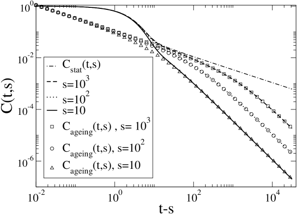
Figure 2: Autocorrelator $C(t,s)$ of the critical $3D$ BCPD ($\eta=2$) as a function of $t-s$, for several values of $s$. Full lines: complete autocorrelator. Dash-dotted line: stationary correlator eq. (5.2). Symbols: scaling contribution $C_{\rm ageing}(t,s)=s^{-b}f_{C}(t/s)$.

For a qualitative overview, we show in figure 2, the autocorrelation function $C(t,s)$ as a function of time separation $t-s$. For small time-separations, the autocorrelator remains close to the quasi-stationary, time-translationally-invariant form implied by the Poissonian initial conditions, before crossing over to the scaling regime with ageing behaviour when $t-s$ becomes large. In order to be able to define a precise measure of this cross-over, we consider the following relative error

$$\delta C(t,s)=\left|\frac{C(t,s)-C_{stat}(t,s)}{C_{ageing}(t,s)-C_{stat}(t,s)}\right|$$ (5.1)

where $C_{stat}(t,s)$ is the quasi-stationary correlation function

$$C_{stat}(t,s)=\alpha\rho_{0}\int_{\frac{t-s}{2}}^{\infty}\!{\rm d}\tau\int_{0}^{\pi}\!{\rm d}q\,q^{d-1}\,\exp\left(\omega(q)\,\tau\right)$$ (5.2)

and $C_{ageing}(t,s)=s^{-b}f_{C}(t/s)$ is the autocorrelator in the ageing regime, see eq. (2.16). Since $0\leq\delta C(t,s)\leq 1$, we arbitrarily consider the system to be in the stationary regime when $\delta C(t,s)<10\%$ and to be in the ageing regime when $\delta C(t,s)>90\%$. In figure 3, this relative error is plotted as a function of the separation time for different values of $s$. We observe that the passage from the quasi-stationary regime to the ageing regime occurs at relatively well-defined transition-times.

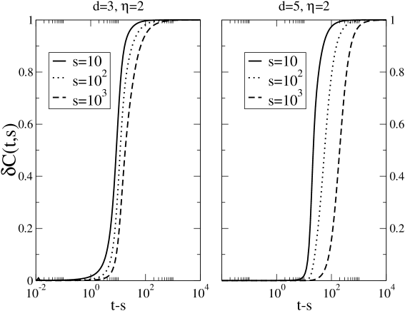
Figure 3: Relative error $\delta C(t,s)$ as a function of time separation $t-s$ for different values of the waiting time $s$ in the BCPD. Left panel: $d=3$, right panel: $d=5$.

Two transition times will be defined:

1. the system leaves the quasi-stationary regime at the time scale $\tau_{\rm stat}(s)$ which is defined by

   $$\delta C(\tau_{\rm stat}(s)+s,s)=0.1$$

2. the system enters the ageing regime at the time scale $\tau_{\rm ageing}(s)$ which is defined by

   $$\delta C(\tau_{\rm ageing}(s)+s,s)=0.9$$

These transition times are shown as a function of the waiting time $s$ for several dimensions in figure 4. We find for sufficiently large $s$ the asymptotic behaviour

$$\tau_{ageing}(t,s)=A\,s^{\zeta}$$ (5.3)

where $A$ depends on dimension and the passage exponent $\zeta<1$. In principle, $\zeta$ should depend on both the dimension $d$ and the Lévy parameter $\eta$. However, as illustrated in figure 5, $\zeta$ apparently depends merely on the ratio $d/\eta$. Indeed, we obtain a neat collapse of the entire curves $\tau_{\rm ageing}(s)$ for different values of $d$ and $\eta$, but with the same value of $d/\eta$. Therefore, it is enough to look at models with a fixed ratio of $d/\eta$ and for that reason most of our calculations were performed for the BCPD.

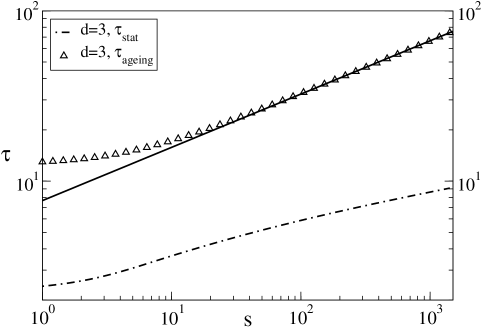
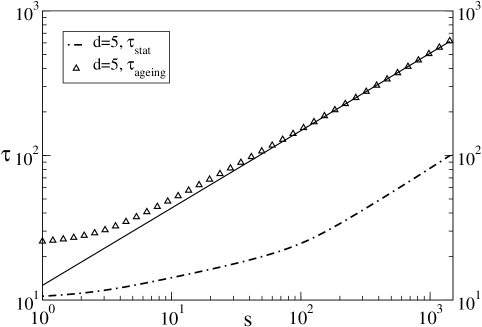
Figure 4: Transition times $\tau_{\rm stat}(s)$ (lower curves) and $\tau_{\rm ageing}(s)$ (upper curves) as a function of $s$ of the BCPD, in $3D$ (left panel) and in $5D$ (right panel). The full lines give the linear fits: $\tau_{\rm ageing}(s)=7.7\cdot s^{0.31}$ for $d=3$ and $\tau_{\rm ageing}(s)=12.6\cdot s^{0.53}$ for $d=5$.

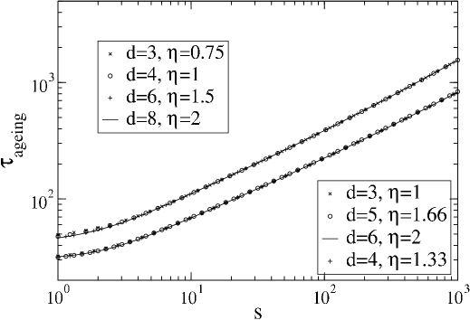
Figure 5: Dependence of the transition time $\tau_{\rm ageing}(s)$ on the ratio $d/\eta$. The upper set of curves corresponds to $d/\eta=4$ and the lower one corresponds to $d/\eta=3$.

The dependence of $\zeta$ on the dimension $d$ is shown for $\eta=2$ in figure 6 and in table 3. Analogously to the study of Zippold et al. [47] for spherical ferromagnets and spherical spin glasses quenched to $T<T_{c}$, our results for the critical passage exponent indicate that $\zeta<1$. In table 3 we list some known values of $\zeta$ (the values for the critical spherical ferromagnet are obtained in appendix C). In conclusion, we find that the same qualitative behaviour for the passage time between the quasi-stationary and the ageing regime, $\tau_{\rm ageing}(s)\sim s^{\zeta}$ with $0<\zeta<1$ apparently holds true both for critical as well as for non-critical systems. This form of the passage time is one of the ingredients for the derivation of admissible scaling forms of the two-time autocorrelator, which gives $C(t,s)=C_{\rm st}(t-s)+C_{\rm age}(t,s)$, where [1]

$$C_{\rm age}(t,s)={\cal C}\left(\frac{h(t)}{h(s)}\right)\;\;,\;\;h(t)=h_{0}\exp\left[\frac{1}{A}\frac{t^{1-\mu}-1}{1-\mu}\right]$$ (5.4)

where $\cal C$ is a scaling function, $\mu$ is a free parameter related to $\zeta$ and $h_{0}$ and $A$ are normalisation constants. However, while for quenches for $T<T_{c}$ the available evidence suggests that $\zeta$ should decrease with $d$, see table 3 [47], we find the opposite tendency for critical quenches, see figure 6 and table 3.

model		condition	$d$	$\zeta$	Ref.
XY		$T=0$	$1$	$2/3$	[22]
spherical		$T<T_{c}$	$>2$	$4/(d+2)$	[47]
$p$-spin spherical glass	$p=2$	$T<T_{c}$	–	$4/5$	[47]
	$p=3$	$T<T_{c}$	–	$\approx 0.68$	[32]
BCPD		$\lambda=\mu$	$3$	$0.31(1)$
			3.5	0.40(1)
			4	0.47(1)
			5	0.53(1)
			6	0.58(1)
spherical		$T=T_{c}$	$3$	$0.33(1)$
			$5$	$0.40(1)$

Table 3: Values of the passage exponent $\zeta$ defined in eq. (5.3) for several models, either in the coexistence phase or at criticality.

Figure 6: Exponent $\zeta$ against dimension $d$ for the BCPD (where $\eta=2$ was used). If $d$ is replaced by $\eta d/2$, the results are also valid of the BCPL.

The passage towards the ageing regime can still be understood heuristically in a different way. At equilibrium, the fluctuation-dissipation theorem (FDT) describes the expected size of the fluctuations, given the response to an external perturbation. If the FDT is broken in ageing phenomena, the inverse fluctuation-dissipation ratio (FDR) describes by how much this expectation is larger than the actually found result, for a given value of the temperature $T$ [33]. Since for the BCPL, the ageing exponents $a=b$ are equal, we can define an analogue of a fluctuation-dissipation ratio

$$X(t,s)=\frac{\frac{\partial C}{\partial s}(s,s)}{R(s,s)}\,\frac{R(t,s)}{\frac{\partial C}{\partial s}(t,s)}$$ (5.5)

but where now the initial FDR plays the role the temperature in system with an equilibrium stationary state. From our exact solution of the BCPL, we find, in the ageing regime

$$X_{\rm ageing}(t,s)=\frac{1}{1+\left(\frac{t-s}{t+s}\right)^{d/\eta}}$$ (5.6)

In figure 7, we show $X(t,s)$ and $X_{\rm ageing}(t,s)$ as a function of the time separation $t-s$ for different waiting times $s$. We can distinguish three different regimes:

1. a quasi-stationary regime with microscopic relaxation for $t-s\ll\tau_{\rm stat}(s)$

2. a non-analytic transition regime for $\tau_{\rm stat}(s)\ll t-s\ll\tau_{\rm ageing}(s)$

3. the ageing regime when $t-s\gg\tau_{\rm ageing}(s)$.

The bold circles in figure 7 indicate the transitions between these regimes. We see that the FDR is still very close to unity when the quasi-stationary regime is left and not too far from its limit value $X_{\infty}=\frac{1}{2}$ upon entering the ageing regime.

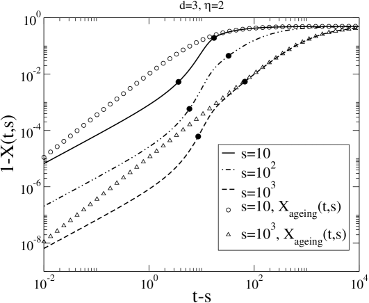
Figure 7: Fluctuation-dissipation ratio $X(t,s)$ (full lines) and the ageing limit $X_{\rm ageing}(t,s)$ (symbols) as a function of the time separation $t-s$ for different value of $s$ in the $3D$ BCPD.

6 Conclusions

In analysing the non-equilibrium dynamical scaling of two ‘bosonic’ particle-reaction models with Lévy-flight transport of individual particles, characterised by the parameter $\eta$, instead of diffusive transport, we have obtained the following results:

1. We have defined the ‘bosonic’ contact and pair-contact processes BCPL and BPCPL. Because of the absence of a ‘fermionic’ constraint limiting the number of particles per site, the models are exactly solvable, either in the full parameter space as the BCPL or along the critical line as the BPCPL. Since the global particle number is conserved on the critical line, information on the nature of the phase transition comes from analysing the variance of the particle distribution. This shows that the BCPL and BPCPL may give rise to a condensation of the particles on essentially a single lattice site.

2. Starting from an initial condition far from the stationary state, the two-time correlation and response functions obey the same kind of dynamical scaling and ageing, see eq. (1.1,1.2) as already found in other systems without detailed balance. The explicit results for the non-equilibrium exponents and the scaling functions are given in tables 1 and 2 for arbitrary values $0<\eta<2$.

   For $\eta=2$ our results include those of the diffusive case (models BCPD and BPCPD [28, 37, 5]) as special cases.

3. We have used these explicit results to test a formulation of local scale-invariance for a dynamical exponent $z=\eta<2$. Extensions of global dynamical scaling to a more local form in non-equilibrium systems must be capable of treating the dynamical symmetries of stochastic Langevin equations, which is done by attempting to perturb around the noiseless, ‘deterministic’ part of the model, which in the case of the BCPL studied here takes the simple Markovian form $\bigl{(}2{\cal M}\partial_{t}-\Delta^{\eta/2}\bigr{)}\phi=0$, where $\cal M$ is a dimensionful constant. Local scale-invariance shows how generalised Bargmann superselection rules can be derived for arbitrary values of the dynamical exponent such that the perturbation series naturally truncates. Our analysis shows how the procedure may be extended to systems without detailed balance and in this sense generalises earlier studies performed on long-ranged ferromagnets [7, 18].

4. Finally, we used the exact solution to follow precisely the passage between the quasi-stationary regime and the late-time ageing regime. In analogy with earlier studies on this passage in non-critical systems [47, 22], our results suggest that the passage time depends on the waiting time $s$ also for critical ferromagnets, as well as for systems without detailed balances, as $\tau_{\rm ageing}(s)\sim s^{\zeta}$, with $0<\zeta<1$.

All in all, the explicit study of the exactly solvable BCPL and BPCPL processes has permitted us to control and to confirm several assumptions, usually admitted in studies of non-equilibrium dynamical scaling, and hence to extend their range of applicability.

Appendix A. Proof of eq. (2.9)

We generalise Baumann’s proof [4], valid for diffusive motion of single particles, to the case of long-range jumps. We work in the quantum hamiltonian/Liouvillian formalism. By the property $\langle s|a^{\dagger}(x)=\langle s|$, we can verify that along the critical line

$$\partial_{t}\langle s|a(\boldsymbol{x})=\langle s|[a(\boldsymbol{x}),H]=\sum_{\mathbb{n}\neq 0}\langle s|D(\boldsymbol{n})\left((a(\boldsymbol{x}+\boldsymbol{n})-a(\boldsymbol{x})\right)$$ (A1)

The Fourier transform is defined as $\langle s|\widetilde{a}({\mathbb{k}})=\sum_{\mathbb{x}}e^{-{\rm i}{\mathbb{k}.x}}\langle s|a({\mathbb{x}})$, therefore

$$\langle s|\widetilde{a}(t,{\mathbb{k}})=\exp\left(-\frac{1}{2}\omega({\mathbb{k}})(t-s)\right)\langle s|\widetilde{a}(s,{\mathbb{k}})$$ (A2)

where $\omega({\mathbb{k}})$ is the dispersion relation. Using Fourier’s theorem $\langle s|a({\mathbb{x}})=(2\pi)^{-d}\int_{B}d{\mathbb{k}}\;e^{-i{\mathbb{k}.x}}\langle s|\tilde{a}({\mathbb{k}x})$, we have for all times $s\leq t$

$$\begin{split}\langle s|a(t,{\mathbb{x}})&=\sum_{\mathbb{y}}\int_{B}\frac{{\rm d}{\mathbb{k}}}{(2\pi)^{d}}\;e^{{\rm i}\boldsymbol{k}\cdot(\boldsymbol{x}-\boldsymbol{y})}\exp\left(-\frac{1}{2}\omega({\mathbb{k}})(t-s)\right)\langle s|a(s,\mathbb{y})\\ &=\sum_{\mathbb{y}}R(t-s;\boldsymbol{x}-\boldsymbol{y})\langle s|a(s,{\mathbb{y}})\end{split}$$ (A3)

where we have used the expression (2.13) of the response function. Next, we apply (A3) to the two-point correlation function

$$F(t,s;{\mathbb{r}})=\langle a(t,{\mathbb{x}})a(s,\mathbb{x}+\boldsymbol{r})\rangle=\sum_{\mathbb{y}}R(t-s;\mathbb{x}-\boldsymbol{y})F(s,\mathbb{r}+\boldsymbol{x}-\boldsymbol{y})$$ (A4)

We also calculate the density-density correlator and we find

$$\begin{split}\langle n(t,{\mathbb{x}})n(s,\mathbb{x}+\boldsymbol{r})\rangle&=\langle a^{\dagger}(t,{\mathbb{x}})a(t,{\mathbb{x}})a^{\dagger}(s,\mathbb{x}+\boldsymbol{r})a(s,\mathbb{x}+\boldsymbol{r})\rangle\\ &=\sum_{\mathbb{y}}R(t-s;\mathbb{x}-\boldsymbol{y})\langle a(t,{\mathbb{x}})a^{\dagger}(s,\mathbb{x+r})a(s,\mathbb{x+r})\rangle\\ &=\sum_{\mathbb{y}}R(t-s;\mathbb{x}-\boldsymbol{y})F(s,\mathbb{r}+\boldsymbol{x}-\boldsymbol{y})+R(t-s;{\mathbb{r}})\rho_{0}\\ &=F(t,s;\boldsymbol{r})+R(t-s;{\mathbb{r}})\rho_{0}\end{split}$$ (A5)

where we have used the time-dependent commutator of $a$ and $a^{\dagger}$ and also applied (A4). Going back to the definition (2.5) the assertion (2.9) follows.

Finally, using the scaling forms (1.1,1.2) together with the exponents of table 1, we explicitly see that the second term in eq. (2.9) becomes negligible compared to the first one in all cases.

Appendix B. Analysis of the correlators

We discuss those aspects in the calculation of the correlators which go beyond the local BCPD and BPCPD models [37, 5]. First, we reconsider the Green’s function $b(t,\boldsymbol{r})$, see eq. (2.11). In the ageing regime ($t,s\gg 1$ et $t-s\gg 1$), only small values of ${\mathbb{q}}$ will contribute. Therefore,

$$b(t,{\mathbb{r}})=\frac{1}{(2\pi)^{d}}\int_{B}\!{\rm d}^{d}{\mathbb{q}}\>e^{\left({\rm i}{\mathbb{q}}\cdot{\mathbb{r}}-\omega({\mathbb{q}})t\right)}\underset{t\rightarrow\infty}{=}\frac{t^{-d/\eta}}{(2\pi)^{d}}\int_{\mathbb{R}^{d}}\!{\rm d}^{d}{\mathbb{q}}\>e^{\left({\rm i}{\mathbb{q}}\cdot{\mathbb{r}}t^{-1/\eta}-\|{\mathbb{q}}\|^{\eta}c\right)}$$ (B1)

From this, we identify the scaling variable ${\mathbb{\xi}}={\mathbb{r}}t^{-1/\eta}$ and read off the dynamical exponent $z=\eta$.

For the explicit calculation of the correlator in the BCPL, we merely have to evaluate eq. (2.16). For the autocorrelator, we find

• Case $d=\eta$:

  $$C(t,s;{\mathbb{0}})=\alpha\rho_{0}B_{0}\int_{\frac{t-s}{2}}^{\frac{t+s}{2}}{\rm d}\tau\>\tau=\alpha\rho_{0}B_{0}\textrm{ ln}\left(\frac{t/s+1}{t/s-1}\right)=f_{C}(t/s)$$ (B2)

  where $B_{0}=\frac{2^{1-d}\Gamma(d/\eta)}{\eta c^{d/\eta}\pi^{d/2}\Gamma(d/2)}$ and we read off the exponents $b=0$ and $\lambda_{C}=d$.

• Case $d\neq\eta$:

  $$C(t,s;\boldsymbol{0}) = \frac{\alpha\rho_{0}B_{0}}{1-d/\eta}\left(\left(\frac{t+s}{2}\right)^{1-d/\eta}-\left(\frac{t-s}{2}\right)^{1-d/\eta}\right)$$ (B3)

  $$\simeq \frac{\alpha\rho_{0}B_{0}}{2^{-d/\eta}}\>s^{1-d/\eta}\left(\frac{t}{s}\right)^{-d/\eta}$$

  and in the second line we looked at the asymptotic form if $t/s\to\infty$. We read off the exponent $b=-1+d/\eta$ and $\lambda_{C}=d$.

The space-time-dependent scaling functions can be found similarly. We merely quote the result:

$$C(t,s;\boldsymbol{r})=\alpha\rho_{0}B_{0}\left(C_{-1}\left(\frac{\boldsymbol{r}}{\left(\frac{t-s}{2}\right)^{1/\eta}}\right)\left(\frac{t-s}{2}\right)^{1-d/\eta}-C_{-1}\left(\frac{\boldsymbol{r}}{\left(\frac{t+s}{2}\right)^{1/\eta}}\right)\left(\frac{t+s}{2}\right)^{1-d/\eta}\right)$$ (B4)

where the function $C_{-1}$ reads

$$C_{-1}(\boldsymbol{r}t^{-1/\eta})=t^{d/\eta}B_{0}^{-1}\int_{\mathbb{R}^{d}}{\rm d}^{d}\boldsymbol{q}\;\;e^{{\rm i}\boldsymbol{q}\cdot\boldsymbol{r}}\;e^{-|\boldsymbol{q}|^{\eta}t}\left(c|q|^{\eta}\right)^{-1}$$ (B5)

For the BPCPL, using Laplace transform on eq (2.17) and applying a similar analysis than in [21], we evaluate $F(t,\boldsymbol{0})$ in the different cases and then use the eq (2.18) to compute the connected correlator. The most interesting cases are $\alpha\leq\alpha_{C}$ and $d>\eta$

1. $\alpha<\alpha_{C}$ and $d>\eta$: here, $F(t,\boldsymbol{0})=\frac{\alpha_{C}\rho_{0}^{2}}{\alpha_{C}-\alpha}$ and the scaling function reads

   $$f_{C}(y)=\frac{\alpha\alpha_{C}\rho_{0}^{2}B_{0}}{(\alpha-\alpha_{C})\left(\frac{2d}{\eta}-2\right)2^{-d/\eta}}\left[(y+1)^{1-d/\eta}-(y-1)^{1-d/\eta}\right]$$ (B6)

2. $\alpha=\alpha_{C}$:
   For $\eta<d<2\eta$, $F(t,\boldsymbol{0})=\frac{\rho_{0}^{2}}{\alpha_{C}B_{0}|\Gamma(1-d/\eta)|\Gamma(d/\eta)}t^{d/\eta-1}$ and the scaling function is given by

   $$f_{C}(y)=\frac{\rho_{0}^{2}}{|\Gamma(1-d/\eta)|\Gamma(d/\eta)d/\eta}\left(\frac{y+1}{2}\right)^{-d/\eta}\;_{2}F_{1}\left(\frac{d}{\eta},\frac{d}{\eta};\frac{d}{\eta}+1;\frac{2}{y+1}\right)$$ (B7)

   For $d>2\eta$

   $$\begin{split}f_{C}(y)=\frac{\rho_{0}^{2}B_{0}\eta}{A_{2}2^{-d/\eta+2}(d-\eta)\left(d-2\eta\right)}\left[2(d-2\eta)\left(y-1\right)^{1-d/\eta}-\eta(y-1)^{2-d/\eta}+\eta(y+1)^{2-d/\eta}\right]\end{split}$$ (B8)

   where $A_{2}=\left(2\int_{B}\frac{{\rm d}^{d}\boldsymbol{q}}{(2\pi)^{d}}(2\omega(\boldsymbol{q}))^{-2}\right)^{-1}$.

3. $\alpha>\alpha_{C}$ or $d<\eta$: $F(t,\boldsymbol{0})$ shows an exponential behaviour and we do not have scaling behaviour in these cases.

The space-time-dependent scaling functions can be found from eq (2.18).

1. $\alpha<\alpha_{C}$ and $d>\eta$:

   $$C(t,s;\boldsymbol{r})=\alpha\rho_{0}B_{0}\left(C_{-1}\left(\frac{\boldsymbol{r}}{\left(\frac{t-s}{2}\right)^{1/\eta}}\right)\left(\frac{t-s}{2}\right)^{1-d/\eta}-C_{-1}\left(\frac{\boldsymbol{r}}{\left(\frac{t+s}{2}\right)^{1/\eta}}\right)\left(\frac{t+s}{2}\right)^{1-d/\eta}\right)$$ (B9)

2. $\alpha=\alpha_{C}$:
   For $\eta<d<2\eta$

   $$C(t,s;\boldsymbol{r})=\frac{\rho_{0}^{2}}{|\Gamma(1-d/\eta)|\Gamma(d/\eta)}\left(\frac{\frac{t}{s}+1}{2}\right)^{-d/\eta}\sum_{n=0}^{\infty}\frac{C_{n}\left(\boldsymbol{r}\left(\frac{t+s}{2}\right)^{-1/\eta}\right)\left(\frac{\frac{t}{s}+1}{2}\right)^{n}}{n!(n+d/\eta)}$$ (B10)

   where $C_{n}$ is defined as

   $$C_{n}(\boldsymbol{r}t^{-1/\eta})=t^{d/\eta}B_{0}^{-1}\int_{\mathbb{R}^{d}}{\rm d}^{d}\boldsymbol{q}\;\;e^{{\rm i}\boldsymbol{q}\cdot\boldsymbol{r}}\;e^{-|\boldsymbol{q}|^{\eta}t}\left(c|q|^{\eta}\right)^{n}$$ (B11)

   For $d>2\eta$

   $$C(t,s;\boldsymbol{r})=\frac{\rho_{0}^{2}}{4A_{2}}B_{0}s^{2-d/\eta}\left(\frac{\frac{t}{s}+1}{2}\right)^{-d/\eta}\sum_{n=0}^{\infty}\frac{C_{n}\left(\boldsymbol{r}\left(\frac{t+s}{2}\right)^{-1/\eta}\right)\left(\frac{\frac{t}{s}+1}{2}\right)^{n}}{n!(n+2)}$$ (B12)

Appendix C. Critical spherical model

We analyse the passage towards the ageing regime in the critical spherical model. As introduced by Berlin and Kac [10], its spins $S_{\boldsymbol{x}}\in\mathbb{R}$ are real variables on a hypercubic lattice $\Lambda$ in $d$ dimensions which obey the so-called spherical constraint

$$\sum_{\boldsymbol{x}\in\Lambda}S^{2}_{\boldsymbol{x}}=\cal{N}$$ (C1)

where $\cal{N}$ is the total number of spins. The dynamics is given by the stochastic Langevin equation

$$\partial_{t}S(t,\boldsymbol{r})=\nabla_{\boldsymbol{r}}^{2}S(t,\boldsymbol{r})+\frac{1}{2}\left(\frac{{\rm d}}{{\rm d}t}\ln g(t)\right)S(t,\boldsymbol{r})+\eta(t,\boldsymbol{r})$$ (C2)

where $\eta(t,\boldsymbol{r})$ is a centred gaussian noise such that $\langle\eta(t,\boldsymbol{r})\eta(t^{\prime},\boldsymbol{r^{\prime}})\rangle=2T_{c}\delta(t-t^{\prime})\delta(\boldsymbol{r}-\boldsymbol{r^{\prime}})$ and $g(t)$ acts as a Lagrange multiplier to enforce the spherical constraint, see below. We only quote from the well-known solution [20] those results we need. The autocorrelation reads (we use an infinite-temperature initial state throughout)

$$C(t,s)=\langle S(t,\boldsymbol{r})S(s,\boldsymbol{r})\rangle=\frac{1}{\sqrt{g(t)g(s)}}\left(f\left(\frac{t+s}{2}\right)+2T_{c}\int_{0}^{s}{\rm d}t^{\prime}f\left(\frac{t+s}{2}-t^{\prime}\right)g(t^{\prime})\right)\\$$ (C3)

where $g(t)$ is given as the solution of the Volterra integral equation

$$g(t)=f(t)+2T_{c}\int_{0}^{t}{\rm d}t^{\prime}f(t-t^{\prime})g(t^{\prime})$$ (C4)

and $f(t)$ reads for short-range interactions ($I_{0}$ is a modified Bessel function)

$$f(t)=\int_{B}\frac{{\rm d}\boldsymbol{q}}{(2\pi)^{d}}e^{-2\omega(\boldsymbol{q})t}=\left(e^{-4t}I_{0}(4t)\right)^{d}$$ (C5)

Finally, the critical temperature $T_{c}$ is given by

$$T_{c}(d)=\left(2\int_{0}^{\infty}{\rm d}t\left(e^{-4t}I_{0}(4t)\right)^{d}\right)^{-1}$$ (C6)

We also recall the scaling functions of the autocorrelator in the ageing regime [20, 21]

$$f_{C}(y) = T_{c}\frac{4(4\pi)^{-d/2}}{(d-2)(y+1)}y^{1-d/4}(y-1)^{1-d/2}\hskip 85.35826pt2<d<4,$$

$$f_{C}(y) = T_{c}\frac{2(4\pi)^{-d/2}}{d-2}\left((y-1)^{1-d/2}-(y+1)^{1-d/2}\right)\hskip 51.21504ptd>4$$ (C7)

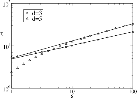
Figure 8: Passage time towards the ageing regime in the spherical model at $T=T_{c}$,as a function of the waiting time $s$, for different values of the dimension $d$. The full lines give the linear fits: $\tau_{\rm ageing}(s)=4.9\cdot s^{0.32}$ for $d=3$ and $\tau_{\rm ageing}(s)=5.2\cdot s^{0.40}$ for $d=5$.

As in the main text, we define the passage times between the quasi-stationary and the ageing regimes. In figure 8, we show $\tau_{\rm ageing}(s)\sim s^{\zeta}$ as a function of $s$. The full curves indicate the numerical solution of the Volterra integral equation (C4) whereas the symbols were obtained from the asymptotic forms (C7). Hence $\tau_{\rm ageing}(s)$ shows the same kind of qualitative behaviour as the BCPL and the resulting values of $\zeta$ are included in table 3.

Acknowledgements XD acknowledges the support by the Centre National de la Recherche Scientifique (CNRS) through grant no. 101160. We thank S.B. Dutta for useful discussions.

References

- [1] A. Andreanov and A. Lefèvre, Europhys. Lett. 76, 919 (2006).
- [2] A.C. Barato and H. Hinrichsen, J. Stat. Mech. P02020 (2009).
- [3] V. Bargmann, Ann. of Math. 56, 1 (1954).
- [4] F. Baumann, Vieillissement et comportement d’échelle dynamique hors équilibre, thèse Nancy & Erlangen (2007)
- [5] F. Baumann, M. Henkel, M. Pleimling and J. Richert, J. Phys. A: Math. Gen. 38, 6623 (2005).
- [6] F. Baumann, S. Stoimenov and M. Henkel, J. Phys. A: Math. Gen. 39, 4095 (2006).
- [7] F. Baumann, S.B. Dutta and M. Henkel, J. Phys. A: Math. Gen. 39, 4095 (2006).
- [8] F. Baumann and A. Gambassi, J. Stat. Mech. P01002 (2007).
- [9] F. Baumann and M. Henkel, en préparation.
- [10] T.H. Berlin and M. Kac, Phys. Rev. 86, 821 (1952)
- [11] A.J. Bray, Adv. Phys. 43, 357 (1994).
- [12] P. Calabrese and A. Gambassi, J. Phys. A: Math. Gen. 38, R133 (2005).
- [13] C. Chamon, L.F. Cugliandolo and H. Yoshino, J. Stat. Mech. P01006 (2006).
- [14] L.F. Cugliandolo, in Slow Relaxation and non equilibrium dynamics in condensed matter, Les Houches Session 77 July 2002, J-L Barrat, J Dalibard, J Kurchan, M V Feigel’man eds (Springer, 2003); also available at cond-mat/0210312.
- [15] C. de Dominicis, J. Physique Colloque 37, 247 (1976).
- [16] O. Deloubrière and F. van Wijland, Phys. Rev. E65, 0461041 (2002).
- [17] M. Doi, J. Phys. A: Math. Gen. 9, 1465 and 1479 (1976).
- [18] S.B. Dutta, J. Phys. A: Math. Theor. 41, 395002, (2008).
- [19] T. Enss, M. Henkel, A. Picone and U. Schollwöck, J. Phys. A: Math. Gen. 37, 10479 (2004).
- [20] C. Godrèche and J.M. Luck, J. Phys. A: Math. Gen. 33, 9141 (2000).
- [21] C. Godrèche and J.M. Luck, J. Phys.: Condens. Matter 14, 1589 (2002).
- [22] C. Godrèche, F. Krzakala and F. Ricci-Tersenghi, J. Stat. Mech. P04007 (2004)
- [23] M. Henkel, Nucl. Phys. B641, 405 (2002).
- [24] M. Henkel, J. Phys.: Condens. Matter 19, 065101 (2007).
- [25] M. Henkel and F. Baumann, J. Stat. Mech. P07015 (2007).
- [26] M. Henkel, H. Hinrichsen and S. Lübeck, Non-equilibrium phase transitions, vol. 1, Springer (Heidelberg 2008).
- [27] H. Hinrichsen and M. Howard, Eur. Phys. J. B7, 635 (1999).
- [28] B. Houchmandzadeh, Phys. Rev. E66, 052902 (2002).
- [29] M. Howard and U.C. Täuber, J. Phys. A: Math. Gen. 30, 7721 (1997).
- [30] H.-K. Janssen, in G. Györgyi et al. (eds) From Phase transitions to Chaos, World Scientific (Singapour 1992), p. 68.
- [31] H.-K. Janssen, K. Oerding, F. van Wijland and H. Hilhorst, Eur. Phys. J. B7, 137 (1999).
- [32] B. Kim and A. Latz, Europhys. Lett. 53, 660 (2001)
- [33] J. Kurchan, Aspects théoriques du vieillissement, in P. Lemoine (éd) Viellissement des métaux, céramiques et matériaux granulaires, EDP Sciences (Les Ulis 2001), p. 1
- [34] I. Lubashevsky, R. Friedrich and A. Heuer arXiv:0905.4472
- [35] R. Metzler and J.Klafter, Phys.Rep 339, 1 (2000)
- [36] G. Ódor, J. Stat. Mech. L11002 (2006).
- [37] M. Paessens and G.M. Schütz, J. Phys. A: Math. Gen. 37, 4709 (2004).
- [38] M. Paessens, cond-mat/0406598.
- [39] W. Paul and J. Baschnagel, Stochastic processes: from physics to finance, Springer (Heidelberg 1999).
- [40] A. Picone and M. Henkel, Nucl. Phys. B688, 217 (2004).
- [41] J.J. Ramasco, M. Henkel, M.A. Santos et C.A. da Silva Santos, J. Phys. A: Math. Gen. 37 10497 (2004).
- [42] G.M. Schütz, in C. Domb and J. Lebowitz (eds) Phase Transitions and Critical Phenomena, Vol. 19, London (Academic 2000), p. 1.
- [43] M.F. Shlesinger, G.M. Zaslavsky and U. Frisch (éd), Lévy flights and related topics in physics, Springer (Heidelberg 1995).
- [44] L.C.E. Struik, Physical ageing in amorphous polymers and other materials, Elsevier (Amsterdam 1978).
- [45] E. Vincent, in M. Henkel, M. Pleimling and R. Sanctuary (eds) Ageing and the glass transition, Springer (Heidelberg 2007), p. 7.
- [46] W.R. Young, A.J. Roberts and G. Stuhne, Nature 412, 328 (2001).
- [47] W. Zippold, R. Kühn and H. Horner, Eur. Phys. J. B13, 531 (2000).