Variational wave functions for frustrated magnetic models

Variational wave functions containing electronic pairing and suppressed charge fluctuations (i.e., projected BCS states) have been proposed as the paradigm for disordered magnetic systems (including spin liquids). Here we discuss the general properties of these states in one and two dimensions, and show that different quantum phases may be described with high accuracy by the same class of variational wave functions, including dimerized and magnetically ordered states. In particular, phases with magnetic order may be obtained from a straightforward generalization containing both antiferromagnetic and superconducting order parameters, as well as suitable spin Jastrow correlations. In summary, projected wave functions represent an extremely flexible tool for understanding the physics of low-dimensional magnetic systems.

0.1 Introduction

The variational approach is a widely used tool to investigate the low-energy properties of quantum systems with several active degrees of freedom, including electrons and ions. The basic idea is to construct fully quantum many-body states by a physically motivated ansatz. The resulting wave function should be simple enough to allow efficient calculations even for large sizes. Most of the variational calculations are traditionally based upon mean-field approximations, where the many-body wave function is constructed by using independent single-particle states. In this respect, even the BCS theory of superconductivity belongs in this category bcs . Although these mean-field approaches have been instrumental in understanding and describing weakly correlated systems, they have proved inadequate whenever the electron-electron interaction dominates the kinetic energy. The generalization of variational states in this regime is not straightforward, and represents an open problem in the modern theory of Condensed Matter. Probably the most celebrated case is the wave function proposed by Laughlin to describe the fractional quantum Hall effect as an incompressible quantum fluid with fractional excitations laughlin . One important example in which electron correlations prevent the use of simple, mean-field approaches is provided by the so-called resonating valence-bond (RVB) state. This intriguing phase, which was conjectured many years ago by Fazekas and Anderson fazekas , has no magnetic order, no broken lattice symmetries, and remains disordered even at zero temperature. It is now commonly accepted that these spin-liquid states may be stabilized in quantum antiferromagnets with competing (frustrating) interactions misguich .

Here we present one possible approach to the definition of accurate variational wave functions which take into account quite readily both strong electron correlations and the frustrated nature of the lattice. The price to pay when considering these effects is that calculations cannot be performed analytically, and more sophisticated numerical methods, such as the quantum Monte Carlo technique, are required.

Let us begin by considering a simple, frustrated spin model, in which the combined effects of a small spin value, reduced dimensionality, and the presence of competing interactions could lead to non-magnetic phases. We consider what is known as the $J_{1}{-}J_{2}$ frustrated Heisenberg model on a chain or a square lattice,

$${\cal H}=J_{1}\sum_{n.n.}{\bf S}_{R}\cdot{\bf S}_{R^{\prime}}+J_{2}\sum_{n.n.n.}{\bf{S}}_{R}\cdot{\bf{S}}_{R^{\prime}},$$ (1)

where $J_{1}$ and $J_{2}$ are the (positive) nearest-neighbor ($n.n.$) and next-nearest-neighbor ($n.n.n.$) couplings, and ${\bf S}_{R}=(S^{x}_{R},S^{y}_{R},S^{z}_{R})$ are $S=1/2$ operators; periodic boundary conditions are assumed. Besides the purely theoretical interest, this model is also known to describe the relevant antiferromagnetic interactions in a variety of quasi-one-dimensional castilla and quasi-two-dimensional systems carretta ; carretta2 .

In one dimension, the phase diagram of the $J_{1}{-}J_{2}$ model has been well established by analytical studies and by Density Matrix Renormalization Group (DMRG) calculations white . For small values of the ratio $J_{2}/J_{1}$, the system is in a Luttinger spin-fluid phase with a gapless spectrum, no broken symmetry, and power-law spin correlations. By increasing the value of the second-neighbor coupling, a gapped phase is stabilized castilla ; white . The value of the critical point has been determined with high accuracy as $(J_{2}/J_{1})_{c}=0.241167\pm 0.000005$ eggert . The gapped ground state is two-fold degenerate and spontaneously dimerized, and at $J_{2}/J_{1}=0.5$ is expressed by the exact Majumdar-Ghosh wave function majumdar1 ; majumdar2 . Interestingly, for $J_{2}/J_{1}>0.5$, incommensurate but short-range spin correlations have been found, whereas the dimer-dimer correlations are always commensurate white .

By contrast, the phase diagram of the two dimensional $J_{1}{-}J_{2}$ model is the subject of much debate. For $J_{2}/J_{1}\ll 0.5$, an antiferromagnetic Néel order with magnetic wave vector $Q=(\pi,\pi)$ is expected. In the opposite limit, $J_{2}/J_{1}\gg 0.5$, the ground state is a collinear antiferromagnetic phase where the spins are aligned ferromagnetically in one direction and antiferromagnetically in the other [$Q=(\pi,0)$ or $Q=(0,\pi)$]. The nature of the ground state in the regime of strong frustration, i.e., for $J_{2}/J_{1}\sim 0.5$, remains an open problem, and there is no general consensus on its characterization. Since the work of Chandra and Doucot doucot , it has been suggested that a non-magnetic phase should be present around $J_{2}/J_{1}=0.5$. Unfortunately, exact diagonalization calculations are limited to small clusters which cannot provide definitive answers to this very delicate problem dagotto ; singh ; schulz . By using series-expansion methods gelfand ; singh2 ; kotov ; sushkov and field-theoretical approaches read , it has been argued that a valence-bond solid, with columnar dimer order and spontaneous symmetry-breaking, could be stabilized. More recently, it has been shown that a clear enhancement of plaquette-plaquette correlations is found by introducing a further, third-nearest-neighbor superexchange term $J_{3}$, thus suggesting a possible plaquette valence-bond crystal mambrini .

The primary obstacle to the characterization of the phase diagram in two dimensions is that the lack of exact results is accompanied, in the frustrated case, by difficulties in applying standard stochastic numerical techniques. Quantum Monte Carlo methods can be applied straightforwardly only to spin-1/2 Hamiltonians of the form (1), with strong restrictions on the couplings (e.g., $J_{1}\geq 0$ and $J_{2}\leq 0$ or $J_{1}\leq 0$ and $J_{2}\leq 0$) in order to avoid a numerical instability known as the sign problem. This is because, in general, quantum Monte Carlo methods do not suffer from numerical instabilities only when it is possible to work with a basis in the Hilbert space where the off-diagonal matrix elements of the Hamiltonian are all non-positive. As an example, in a quantum antiferromagnet with $J_{1}\geq 0$ and $J_{2}=0$ on a bipartite lattice, after the unitary transformation

$${\cal U}^{\dagger}=\exp{\Big{[}-i\pi\sum_{R\in{\rm B}}S_{R}^{z}\Big{]}}$$ (2)

(${\rm B}$ being one of the two sublattices), the transformed Hamiltonian has non-positive off-diagonal matrix elements in the basis $|x\rangle$ whose states are specified by the value of $S_{R}^{z}$ on each site, and $\sum_{R}S_{R}^{z}=S$ lieb . This implies that the ground state of $\cal{U}\cal{H}\cal{U}^{\dagger}$, $|\tilde{\Psi}_{0}\rangle=\sum_{x}\tilde{\Psi}_{0}(x)|x\rangle$, has all-positive amplitudes, $\tilde{\Psi}_{0}(x)>0$, meaning that there exists a purely bosonic representation of the ground state. This property leads to the well-known Marshall-Peierls sign rule lieb ; marshall for the phases of the ground state of ${\cal H}$, ${\rm sign}\{\Psi_{0}(x)\}=(-1)^{N_{\uparrow}(x)}$, where $N_{\uparrow}(x)$ is the number of up spins on one of the two sublattices. The Marshall-Peierls sign rule holds for the unfrustrated Heisenberg model and even for the $J_{1}{-}J_{2}$ chain at the Majumdar-Ghosh point. However, in the regime of strong frustration, the Marshall-Peierls sign rule is violated dramatically richter , and, because no analogous sign rule appears to exist, the ground-state wave function has non-trivial phases. This property turns out to be a crucial ingredient of frustration.

In this respect, a very useful way to investigate the highly frustrated regime is to consider variational wave functions, whose accuracy can be assessed by employing stable (but approximate) Monte Carlo techniques such as the fixed-node approach ceperley . Variational wave functions can be very flexible, allowing the description of magnetically ordered, dimerized, and spin-liquid states. In particular, it is possible to construct variational states with non-trivial signs for the investigation of the strongly frustrated regime.

In the following, we will describe in detail the case in which the variational wave function is constructed by projecting fermionic mean-field states anderson2 . Variational calculations can be treated easily by using standard Monte Carlo techniques. This is in contrast to variational states based on a bosonic representation, which are very difficult to handle whenever the ground state has non-trivial phases liang . Indeed, variational Monte Carlo calculations based on bosonic wave functions suffer from the sign problem in the presence of frustration sindzingre , and stable numerical simulations can be performed only in special cases, for example in bipartite lattices when the valence bonds only connect opposite sublattices liang . Another advantage of the fermionic representation is that the mean-field Hamiltonian allows one to have a simple and straightforward representation also for the low-lying excited states (see the discussion in section 0.6.1, and also Ref. becca for a frustrated model on a three-leg ladder).

0.2 Symmetries of the wave function: general properties

We define the class of projected-BCS (pBCS) wave functions on an $N$-site lattice, starting from the ground state of a suitable translationally invariant BCS Hamiltonian

$${\cal H}_{BCS} = \sum_{R,R^{\prime}\sigma}(t_{R-R^{\prime}}-\mu\,\delta_{R-R^{\prime}})\,c^{\dagger}_{R,\sigma}c_{R^{\prime},\sigma}-\sum_{R,R^{\prime}}\Delta_{R-R^{\prime}}\,c^{\dagger}_{R,\uparrow}c^{\dagger}_{R^{\prime},\downarrow}+H.c.$$ (3)

$$= \sum_{k\sigma}(\epsilon_{k}-\mu)\,c^{\dagger}_{k,\sigma}c_{k,\sigma}-\sum_{k}\Delta_{k}c^{\dagger}_{k,\uparrow}c^{\dagger}_{-k,\downarrow}+H.c.,$$

where $c^{\dagger}_{R,\sigma}$ ($c_{R,\sigma}$) creates (destroys) an electron at site $R$ with spin $\sigma$, the bare electron band $\epsilon_{k}$ is a real and even function of $k$, and $\Delta_{k}$ is also taken to be even to describe singlet electron pairing. In order to obtain a class of non-magnetic, translationally invariant, and singlet wave functions for spin-1/2 models, the ground state $|BCS\rangle$ of Hamiltonian (3) is projected onto the physical Hilbert space of singly-occupied sites by the Gutzwiller operator $P_{G}=\prod_{R}(n_{R,\uparrow}-n_{R,\downarrow})^{2}$, $n_{R,\sigma}$ being the local density. Thus

$$|pBCS\rangle=P_{G}\,|BCS\rangle=P_{G}\prod_{k}(u_{k}+v_{k}c^{\dagger}_{k,\uparrow}c^{\dagger}_{-k,\downarrow})|0\rangle,$$ (4)

where the product is over all the $N$ wave vectors in the Brillouin zone. The diagonalization of Hamiltonian (3) gives explicitly

$$u_{k}=\sqrt{\frac{E_{k}+\epsilon_{k}}{2E_{k}}}\qquad\qquad v_{k}=\frac{\Delta_{k}}{|\Delta_{k}|}\sqrt{\frac{E_{k}-\epsilon_{k}}{2E_{k}}}\qquad\qquad E_{k}=\sqrt{\epsilon_{k}^{2}+|\Delta_{k}|^{2}},$$

while the BCS pairing function $f_{k}$ is given by

$$f_{k}=\frac{v_{k}}{u_{k}}=\frac{\Delta_{k}}{\epsilon_{k}+E_{k}}.$$ (5)

The first feature we wish to discuss is the redundancy implied by the electronic representation of a spin state, by which is meant the extra symmetries which appear when we write a spin state as the Gutzwiller projection of a fermionic state. This property is reflected in turn in the presence of a local gauge symmetry of the fermionic problem affleck ; rice ; wen . Indeed, the original spin Hamiltonian (1) is invariant under the local SU(2) gauge transformations

$$\Sigma^{z}_{\phi}:\left(\begin{array}[]{c}c^{\dagger}_{\uparrow}\cr c_{\downarrow}\end{array}\right)\to e^{i\phi{\bf\sigma}_{z}}\left(\begin{array}[]{c}c^{\dagger}_{\uparrow}\cr c_{\downarrow}\end{array}\right)=\left(\begin{array}[]{cc}e^{i\phi}&0\cr 0&e^{-i\phi}\end{array}\right)\left(\begin{array}[]{c}c^{\dagger}_{\uparrow}\cr c_{\downarrow}\end{array}\right),$$ (14)

$$\Sigma^{x}_{\theta}:\left(\begin{array}[]{c}c^{\dagger}_{\uparrow}\cr c_{\downarrow}\end{array}\right)\to e^{i\theta{\bf\sigma}_{x}}\left(\begin{array}[]{c}c^{\dagger}_{\uparrow}\cr c_{\downarrow}\end{array}\right)=\left(\begin{array}[]{cc}\cos\theta&i\sin\theta\cr i\sin\theta&\cos\theta\end{array}\right)\left(\begin{array}[]{c}c^{\dagger}_{\uparrow}\cr c_{\downarrow}\end{array}\right).$$ (23)

A third transformation can be expressed in terms of the previous ones,

$$\Sigma^{y}_{\psi}:\left(\begin{array}[]{c}c^{\dagger}_{\uparrow}\cr c_{\downarrow}\end{array}\right)\to e^{i\psi{\bf\sigma}_{y}}\left(\begin{array}[]{c}c^{\dagger}_{\uparrow}\cr c_{\downarrow}\end{array}\right)=e^{-i\pi{\bf\sigma}_{z}/4}e^{i\psi{\bf\sigma}_{x}}e^{i\pi{\bf\sigma}_{z}/4}\left(\begin{array}[]{c}c^{\dagger}_{\uparrow}\cr c_{\downarrow}\end{array}\right),$$ (24)

where ${\bf\sigma}_{x}$, ${\bf\sigma}_{y}$, and ${\bf\sigma}_{z}$ are the Pauli matrices. As a consequence, all the different fermionic states connected by a local SU(2) transformation generated by (14) and (23) with site-dependent parameters give rise to the same spin state after Gutzwiller projection,

$$P_{G}\,\prod_{R}\Sigma^{z}_{\phi_{R}}\Sigma^{x}_{\theta_{R}}\,|BCS\rangle=e^{i\Phi}P_{G}\,|BCS\rangle,$$ (25)

where $\Phi$ is an overall phase. Clearly, the local gauge transformations defined previously change the BCS Hamiltonian, breaking in general the translational invariance. In the following, we will restrict our considerations to the class of transformations which preserve the translational symmetry of the lattice in the BCS Hamiltonian, i.e., the subgroup of global symmetries corresponding to site-independent angles $(\phi,\theta)$. By applying the transformations (14) and (23), the BCS Hamiltonian retains its form with modified couplings

$$t_{R-R^{\prime}} \to t_{R-R^{\prime}}$$ (26)

$$\Delta_{R-R^{\prime}} \to \Delta_{R-R^{\prime}}e^{2i\phi}$$ (27)

for $\Sigma^{z}_{\phi}$, while the transformation $\Sigma^{x}_{\theta}$ gives

$$t_{R-R^{\prime}} \to \cos 2\theta\,t_{R-R^{\prime}}+i\sin\theta\cos\theta\,(\Delta_{R-R^{\prime}}-\Delta^{*}_{R-R^{\prime}})$$ (28)

$$= \cos 2\theta\,t_{R-R^{\prime}}-\sin 2\theta\,{\rm Im}\Delta_{R-R^{\prime}}$$

$$\Delta_{R-R^{\prime}} \to (\cos^{2}\theta\,\Delta_{R-R^{\prime}}+\sin^{2}\theta\,\Delta^{*}_{R-R^{\prime}})+i\sin 2\theta\,t_{R-R^{\prime}}$$ (29)

$$= {\rm Re}\Delta_{R-R^{\prime}}+i\left(\cos 2\theta\,{\rm Im}\Delta_{R-R^{\prime}}+\sin 2\theta\,t_{R-R^{\prime}}\right).$$

These relations are linear in $t_{R-R^{\prime}}$ and $\Delta_{R-R^{\prime}}$, and therefore hold equally for the Fourier components $\epsilon_{k}$ and $\Delta_{k}$. We note that, because $\Delta_{r}$ is an even function, the real (imaginary) part of its Fourier transform $\Delta_{k}$ is equal to the Fourier transform of the real (imaginary) part of $\Delta_{r}$. It is easy to see that these two transformations generate the full rotation group on the vector whose components are $(\epsilon_{k},\,{\rm Re}\Delta_{k},\,{\rm Im}\Delta_{k})$. As a consequence, the length $E_{k}$ of this vector is conserved by the full group.

In summary, there is an infinite number of different translationally invariant BCS Hamiltonians that, after projection, give the same spin state. Choosing a specific representation does not affect the physics of the state, but changes the pairing function $f_{k}$ of Eq. (5) before projection. Within this class of states, the only scalar under rotations is the BCS energy spectrum $E_{k}$. Clearly, the projection operator will modify the excitation spectrum associated with the BCS wave function. Nevertheless, its invariance with respect to SU(2) transformations suggests that $E_{k}$ may reflect the nature of the physical excitation spectrum.

Remarkably, in one dimension it is easy to prove that such a class of wave functions is able to represent faithfully both the physics of Luttinger liquids, appropriate for the nearest-neighbor Heisenberg model, and the gapped spin-Peierls state, which is stabilized for sufficiently strong frustration. In fact, it is known haldane that the simple choice of nearest-neighbor hopping ($\epsilon_{k}=-2t\,\cos k$, $\mu=0$) and vanishing gap function $\Delta_{k}$ reproduces the exact solution of the Haldane-Shastry model (with a gapless $E_{k}$), while choosing a next-nearest neighbor hopping ($\epsilon_{k}=-2t\,\cos 2k$, $\mu=0$) and a sizable nearest-neighbor pairing ($\Delta_{k}=4\sqrt{2}t\,\cos k$) recovers the Majumdar-Ghosh state (with a gapped $E_{k}$) majumdar1 ; majumdar2 .

0.3 Symmetries in the two-dimensional case

We now specialize to the two-dimensional square lattice and investigate whether it is possible to exploit further the redundancy in the fermionic representation of a spin state in order to define a pairing function which breaks some spatial symmetry of the lattice but which, after projection, still gives a wave function with all of the correct quantum numbers. We will show that, if suitable conditions are satisfied, a fully symmetric projected BCS state is obtained from a BCS Hamiltonian with fewer symmetries than the original spin problem. For this purpose, it is convenient to introduce a set of unitary operators related to the symmetries of the model.

• Spatial symmetries: for example, ${\cal R}_{x}(x,y)=(x,-y)$ and ${\cal R}_{xy}(x,y)=(y,x)$. We define the transformation law of creation operators as ${\cal R}c^{\dagger}_{X,\sigma}{\cal R}^{-1}=c^{\dagger}_{{\cal R}(X),\sigma}$, and the action of the symmmetry operator on the vacuum is ${\cal R}_{x}|0\rangle={\cal R}_{xy}|0\rangle=|0\rangle$. Note that these operators map each sublattice onto itself.

• Particle-hole symmetry: $P_{h}c^{\dagger}_{X,\sigma}P_{h}^{-1}=i\,(-1)^{X}c_{X,-\sigma}$, where the action of the $P_{h}$ operator on the vacuum is $P_{h}|0\rangle=\prod_{X}c^{\dagger}_{X,\uparrow}c^{\dagger}_{X,\downarrow}|0\rangle$.

• Gauge transformation: $G\,c^{\dagger}_{X,\sigma}G^{-1}=i\,c^{\dagger}_{X,\sigma}$ with $G\,|0\rangle=|0\rangle$.

Clearly, ${\cal R}_{x}$ and ${\cal R}_{xy}$ are symmetries of the physical problem (e.g., the Heisenberg model). $G$ is a symmetry because the physical Hamiltonian has a definite number of electrons, while $P_{h}$ leaves invariant every configuration where each site is singly occupied if the total magnetization vanishes ($N_{\downarrow}=N_{\uparrow}=n$). With the definition adopted, $P_{h}$ acts only to multiply every spin state by the phase factor $(-1)^{N_{\downarrow}}$. Thus all of the operators defined above commute both with the Heisenberg Hamiltonian and, because reflections do not interchange the two sublattices, with each other. The ground state of the Heisenberg model on a finite lattice, if it is unique, must be a simultaneous eigenstate of all the symmetry operators. We will establish the sufficient conditions which guarantee that the projected BCS state is indeed an eigenstate of all of these symmetries.

Let us consider a hopping term which only connects sites in opposite sublattices, whence $\epsilon_{k+Q}=-\epsilon_{k}$, and a gap function with contributions from different symmetries ($s$, $d_{x^{2}-y^{2}}$, and $d_{xy}$), $\Delta=\Delta^{s}+\Delta^{x^{2}-y^{2}}+\Delta^{xy}$. Further, we consider a case in which $\Delta^{s}$ and $\Delta^{x^{2}-y^{2}}$ couple opposite sublattices, while $\Delta^{xy}$ is restricted to the same sublattice. In this case, the BCS Hamiltonian ${\cal H}_{BCS}={\cal H}(t,\Delta^{s},\Delta^{x^{2}-y^{2}},\Delta^{xy})$ transforms under the different unitary operators acording to

$${\cal R}_{x}{\cal H}(t,\Delta^{s},\Delta^{x^{2}-y^{2}},\Delta^{xy}){\cal R}_{x}^{-1} = {\cal H}(t,\Delta^{s},\Delta^{x^{2}-y^{2}},-\Delta^{xy}),$$

$${\cal R}_{xy}{\cal H}(t,\Delta^{s},\Delta^{x^{2}-y^{2}},\Delta^{xy}){\cal R}_{xy}^{-1} = {\cal H}(t,\Delta^{s},-\Delta^{x^{2}-y^{2}},\Delta^{xy}),$$

$$P_{h}{\cal H}(t,\Delta^{s},\Delta^{x^{2}-y^{2}},\Delta^{xy})P_{h}^{-1} = {\cal H}(t,{\Delta^{s}}^{*},{\Delta^{x^{2}-y^{2}}}^{*},-{\Delta^{xy}}^{*}),$$

$$G{\cal H}(t,\Delta^{s},\Delta^{x^{2}-y^{2}},\Delta^{xy})G^{-1} = {\cal H}(t,-\Delta^{s},-\Delta^{x^{2}-y^{2}},-\Delta^{xy}).$$

From these transformations it is straightforward to define suitable composite symmetry operators which leave the BCS Hamiltonian invariant. For illustration, in the case where $\Delta$ is real, one may select ${\cal R}_{x}P_{h}$ and ${\cal R}_{xy}$ if $\Delta^{x^{2}-y^{2}}=0$ or ${\cal R}_{x}P_{h}$ and ${\cal R}_{xy}P_{h}G$ if $\Delta^{s}=0$. It is not possible to set both $\Delta^{x^{2}-y^{2}}$ and $\Delta^{s}$ simultaneously different from zero and still obtain a state with all the symmetries of the original problem. The eigenstates $|BCS\rangle$ of Eq. (3) will in general be simultaneous eigenstates of these two composite symmetry operators with given quantum numbers, for example $\alpha_{x}$ and $\alpha_{xy}$. The effect of projection over these states is

$$\alpha_{x}\,P_{G}|BCS\rangle = P_{G}{\cal R}_{x}P_{h}|BCS\rangle={\cal R}_{x}P_{h}P_{G}|BCS\rangle$$ (30)

$$= (-1)^{n}{\cal R}_{x}P_{G}|BCS\rangle,$$

where we have used that both ${\cal R}_{x}$ and $P_{h}$ commute with the projector. Analogously, when a term $\Delta_{x^{2}-y^{2}}$ is present,

$$\alpha_{xy}\,P_{G}|BCS\rangle = P_{G}{\cal R}_{xy}P_{h}G|BCS\rangle={\cal R}_{xy}P_{h}GP_{G}|BCS\rangle$$ (31)

$$= {\cal R}_{xy}P_{G}|BCS\rangle.$$

These equations show that the projected BCS state with both $s$ and $d_{xy}$, or $d_{x^{2}-y^{2}}$ and $d_{xy}$, contributions to the gap has definite symmetry under reflections, in addition to being translationally invariant. The corresponding eigenvalues, for $n=N/2$ even, coincide with the eigenvalues of the modified symmetry operators ${\cal R}_{x}P_{h}$ and ${\cal R}_{xy}P_{h}G$ on the pure BCS state.

In the previous discussion of quantum numbers, it was assumed that $u_{k}$ and $v_{k}$ are well defined for every wave vector $k$. However, this condition is in general violated: singular $k$-points are present whenever both the band structure $\epsilon_{k}$ and the gap function $\Delta_{k}$ vanish, as for example with $\mu=0$, nearest-neighbor hopping and $d_{x^{2}-y^{2}}$ pairing at $k=(\pm\frac{\pi}{2},\pm\frac{\pi}{2})$. However, on finite lattices, this occurrence can be avoided by the choice of suitable boundary conditions. In fact we are free to impose either periodic or antiperiodic boundary conditions on the fermionic BCS Hamiltonian (3), while maintaining all the symmetries of the original lattice. In our studies we have selected lattices and boundary conditions which do not result in singular $k$-points. We note that the quantum numbers of the projected state do depend in general on the choice of boundary conditions in the fermionic BCS Hamiltonian.

0.3.1 The Marshall-Peierls sign rule

Another interesting property of the class of pBCS wave functions is related to the possibility of satisfying the Marshall-Peierls sign rule by means of a suitable choice of the gap function. In particular, we will restrict our considerations to the class of projected wave functions specified in Eq. (4) when both $t_{R-R^{\prime}}$ and $\Delta_{R-R^{\prime}}$ are real and couple sites in opposing sublattices. We begin with the BCS Hamiltonian (3) and perform a particle-hole transformation on the down spins alone, $d^{\dagger}_{R,\uparrow}=c^{\dagger}_{R,\uparrow}$ and $d^{\dagger}_{R,\downarrow}=e^{iQ\cdot R}c_{R,\downarrow}$, with $Q=(\pi,\pi)$, followed by the canonical transformation (spin rotation) $a_{+}(k)=(d_{k,\uparrow}+id_{k,\downarrow})/\sqrt{2}$ and $a_{-}(k)=-i(d_{k,\uparrow}-id_{k,\downarrow})/\sqrt{2}$. The BCS Hamiltonian then acquires the form

$${\cal H}_{BCS}=\sum_{k}\left[h_{+}(k)+h_{-}(k)\right],$$ (32)

where $h_{\pm}(k)=\epsilon_{k}a_{\pm}^{\dagger}(k)a_{\pm}(k)\pm i\Delta_{k}a_{\pm}^{\dagger}(k)a_{\pm}(k+Q)$, and we have used the symmetry $\Delta_{k}=-\Delta_{k+Q}$. Due to the anticommutation rules of the operators $a_{\pm}(k)$, the ground state of ${\cal H}_{BCS}$ can be written as a tensor product of free states of $\pm$ fermions. Moreover, if $\sum_{R}\Psi(R_{1}\cdots R_{n})a_{+}^{\dagger}(R_{1})\cdots a_{+}^{\dagger}(R_{n})|0\rangle$ is the ground state of $\sum_{k}h_{+}(k)$, then $\sum_{R}\Psi^{*}(R_{1}\cdots R_{n})a_{-}^{\dagger}(R_{1})\cdots a_{-}^{\dagger}(R_{n})|0\rangle$ is the ground state of $\sum_{k}h_{-}(k)$. Here we have chosen an arbitrary ordering of the lattice sites. The ground state of ${\cal H}_{BCS}$ is therefore

$$\sum_{R,R^{\prime}}\Psi(R_{1}\cdots R_{n})\Psi^{*}(R^{\prime}_{1}\cdots R^{\prime}_{n})a^{\dagger}_{+}(R_{1})\cdots a^{\dagger}_{+}(R_{n})a^{\dagger}_{-}(R^{\prime}_{1})\cdots a^{\dagger}_{-}(R^{\prime}_{n})|0\rangle.$$ (33)

If this state is expressed in terms of the original electron operators we obtain, up to a factor of proportionality,

$$\sum_{R,R^{\prime}}\Psi(R_{1}\cdots R_{n})\Psi^{*}(R^{\prime}_{1}\cdots R^{\prime}_{n})\left[c^{\dagger}_{R_{1},\uparrow}-ie^{iQ\cdot R_{1}}c_{R_{1},\downarrow}\right]\cdots$$

$$\left[c^{\dagger}_{R^{\prime}_{1},\uparrow}+ie^{iQ\cdot R^{\prime}_{1}}c_{R^{\prime}_{1},\downarrow}\right]\cdots c^{\dagger}_{1,\downarrow}\cdots c^{\dagger}_{N,\downarrow}|0\rangle.$$ (34)

In projecting over the state of fixed particle number equal to the number of sites, we must take the same number of creation and annihilation operators in the $N$ factors of the product. The suppression of doubly occupied sites mandated by the Gutzwiller projector is effected by creating an up spin on sites where a down spin has already been annihilated. The only terms which survive are then those with $\{R\}=\{R^{\prime}\}$, namely

$$\sum_{R}|\Psi(R_{1}\cdots R_{n})|^{2}e^{i\sum_{j}Q\cdot R_{j}}c^{\dagger}_{R_{1},\uparrow}c_{R_{1},\downarrow}\cdots c^{\dagger}_{R_{n},\uparrow}c_{R_{n},\downarrow}\cdots c^{\dagger}_{1,\downarrow}\cdots c^{\dagger}_{N,\downarrow}|0\rangle.$$ (35)

Finally, by moving the down-spin creation operators to the left, one may order the operators according to the specified ordering of the sites in the lattice, independently of the spin, without introducing any further phase factors. On this basis, the resulting wave function has exactly the Marshall-Peierls sign.

0.3.2 Spin correlations

Finally, we would like to calculate the form of the long-range decay of the spin correlations in a BCS state. Here, we will show only that the pure BCS state before projection is characterized by correlations which maintain the symmetries of the lattice even when the BCS Hamiltonian breaks the reflection symmetries due to the presence of both $\Delta^{x^{2}-y^{2}}$ and $\Delta^{xy}$ couplings. Because the BCS state (4) is a translationally invariant singlet, it is sufficient to calculate the longitudinal correlations $\langle S^{z}_{r}S^{z}_{0}\rangle$. A straightforward application of Wick’s theorem leads (for $r\neq 0$) to

$$\langle S^{z}_{r}S^{z}_{0}\rangle \propto -\left[g^{2}(r)+h^{2}(r)\right],$$ (36)

$$g(r) = \int d^{2}k\,{\epsilon_{k}\over E_{k}}\,e^{ik\cdot r},$$ (37)

$$h(r) = \int d^{2}k\,{\Delta_{k}\over E_{k}}\,e^{ik\cdot r}.$$ (38)

Note that when the gap function $\Delta_{k}$ has both $d_{x^{2}-y^{2}}$ and $d_{xy}$ contributions, the correlation function apparently breaks rotational invariance. Equation (36) can be written equivalently in Fourier space as

$$S(q)=\langle S^{z}_{q}S^{z}_{-q}\rangle\,\propto\int d^{2}k\,{\epsilon_{k}\epsilon_{k+q}+\Delta_{k}\Delta_{k+q}\over\sqrt{\Big{[}\epsilon_{k}^{2}+\Delta_{k}^{2}\Big{]}\,\,\left[\epsilon_{k+q}^{2}+\Delta_{k+q}^{2}\right]}}.$$ (39)

Now the effect of an $x$-reflection ${\cal R}_{x}$ on the wave vector $q$ can be deduced by setting $\Delta_{k}=\Delta^{x^{2}-y^{2}}_{k}+\Delta^{xy}_{k}$ and changing the dummy integration variable $k\to{\cal R}_{x}\,(k+Q)$, whence $\Delta_{k+Q}=-\Delta^{x^{2}-y^{2}}_{k}+\Delta^{xy}_{k}$ and $\Delta_{R_{x}k}=\Delta^{x^{2}-y^{2}}_{k}-\Delta^{xy}_{k}$. The net result of these transformations is simply $S({\cal R}_{x}q)=S(q)$, demonstrating that the spin correlations of a BCS state are isotropic, even if the gap function breaks rotational invariance before Gutzwiller projection.

The explicit evaluation of the long-range decay of $g(r)$ for a $d_{x^{2}-y^{2}}$ gap shows that spin correlations in a BCS state (i.e., before projection) display a power-law decay due to the presence of gapless modes: $\langle S^{z}_{r}S^{z}_{0}\rangle\sim 1/r^{4}$ for sites on opposite sublattices, while $\langle S^{z}_{r}S^{z}_{0}\rangle$ vanishes for sites on the same sublattice. A similar result is also expected in the presence of a finite $\Delta^{xy}_{k}$, because gapless modes are present also in this case.

0.4 Connection with the bosonic representation

We turn now to a detailed discussion of the relation between the fermionic anderson2 and bosonic liang representations of the RVB wave function. Recently, bosonic RVB wave functions have been reconsidered by Beach and Sandvik lou ; sandvik ; sandvik2 ; beach . In particular, it has been possible to improve the earlier results of Ref. liang , either by assuming some asymptotic form of the bond distribution beach or by unconstrained numerical methods lou . This wave function has been demonstrated to be extremely accurate for the unfrustrated model with $J_{2}=0$ liang ; lou .

In the fermionic representation, we have

$$|pBCS\rangle=P_{G}\exp\left[\sum_{R<R^{\prime}}f_{R,R^{\prime}}(c^{\dagger}_{R,\uparrow}c^{\dagger}_{R^{\prime},\downarrow}+c^{\dagger}_{R^{\prime},\uparrow}c^{\dagger}_{R,\downarrow})\right]|0\rangle,$$ (40)

where $P_{G}$ projects onto the physical subspace with one electron per site and $f_{R,R^{\prime}}$ is the pairing function, given by the Fourier transform of Eq. (5). The constraint $R<R^{\prime}$ implies the definition of an (arbitrary) ordering of the lattice sites: here and in the following, we will refer to the lexicographical order. For simplicity, let us denote the singlet operator as $\Theta_{R,R^{\prime}}=(c^{\dagger}_{R,\uparrow}c^{\dagger}_{R^{\prime},\downarrow}+c^{\dagger}_{R^{\prime},\uparrow}c^{\dagger}_{R,\downarrow})$. Once the Gutzwiller projector is taken into account, we have that

$$|pBCS\rangle=\sum_{R_{1}<\dots<R_{n}}\,\sum_{P(R^{\prime})}f_{R_{1},R^{\prime}_{1}}\dots f_{R_{n},R^{\prime}_{n}}\Theta_{R_{1},R^{\prime}_{1}}\dots\Theta_{R_{n},R^{\prime}_{n}}|0\rangle,$$ (41)

where $n=N/2$ and $P(R^{\prime})$ represents the permutations of the $n$ sites $R^{\prime}_{k}$ not belonging to the set $\{R\}$, satisfying $R_{k}<R^{\prime}_{k}$ for every $k$. The sum defines all the $(N-1)!!$ partitions of the $N$ sites into pairs.

On the other hand, the bosonic RVB wave function may be expressed in terms of the spin-lowering operator, $S^{-}_{R}$, as

$$|RVB\rangle=\sum_{R_{1}<\dots<R_{n}}\,\sum_{P(R^{\prime})}f^{bos}_{R_{1},R^{\prime}_{1}}\dots f^{bos}_{R_{n},R^{\prime}_{n}}(S^{-}_{R^{\prime}_{1}}-S^{-}_{R_{1}})\dots(S^{-}_{R^{\prime}_{n}}-S^{-}_{R_{n}})|F\rangle,$$ (42)

where the sum has the same restrictions as before and $|F\rangle$ is the (fully polarized) ferromagnetic state. In the bosonic representation, a valence-bond singlet is antisymmetric on interchanging the two sites and, therefore, a direction must be specified. The condition $R_{k}<R^{\prime}_{k}$ fixes the phase (i.e., the sign) of the RVB wave function. In order to make contact between the two representations, we express $|F\rangle$ and $S^{-}_{R}$ in terms of fermionic operators, namely $|F\rangle=c^{\dagger}_{1,\uparrow}\dots c^{\dagger}_{N,\uparrow}|0\rangle$ and $S^{-}_{R}=c^{\dagger}_{R,\downarrow}c_{R,\uparrow}$. Then

$$|RVB\rangle=\sum_{R_{1}<\dots<R_{n}}\,\sum_{P(R^{\prime})}\,\epsilon_{\{R,R^{\prime}\}}f^{bos}_{R_{1},R^{\prime}_{1}}\dots f^{bos}_{R_{n},R^{\prime}_{n}}\Theta_{R_{1},R^{\prime}_{1}}\dots\Theta_{R_{n},R^{\prime}_{n}}|0\rangle,$$ (43)

where $\epsilon_{\{R,R^{\prime}\}}=\pm 1$ is a configuration-dependent sign arising from the reordering of the fermionic operators $(1,\dots N)\to(R_{1},R^{\prime}_{1}\dots R_{n},R^{\prime}_{n})$. The two representations are therefore equivalent only if

$$\epsilon_{\{R,R^{\prime}\}}\,f_{R_{1},R^{\prime}_{1}}\dots f_{R_{n},R^{\prime}_{n}}=f^{bos}_{R_{1},R^{\prime}_{1}}\dots f^{bos}_{R_{n},R^{\prime}_{n}}$$ (44)

for all the valence-bond configurations. In general, for a given $f^{bos}_{R,R^{\prime}}$, this condition cannot be satisfied by any choice of $f_{R,R^{\prime}}$. Remarkably, this is however possible for the short-range RVB state sutherland ; chakraborty , where only nearest-neighbor sites are coupled by $f^{bos}_{R_{k},R^{\prime}_{k}}=1$. Indeed, by using the Kasteleyn theorems kasteleyn , it is possible to prove that Eq. (44) can be fulfilled on all planar graphs (for example in short-range RVB states on lattices with open boundary conditions). In fact, the left-hand side of Eq. (44) is a generic term in the Pfaffian of the matrix

$$M(R,R^{\prime})=\cases{\;\;f_{R,R^{\prime}}&for $R<R^{\prime}$,\cr-f_{R^{\prime},R}&for $R>R^{\prime}$.}$$ (45)

As a consequence, following the arguments of Kasteleyn, it is always possible to orient all the bonds in such a way that in all cycles of the transition graph the number of bonds oriented in either directions is odd kasteleyn . Notice that the latter way to orient the bonds will in general be different from the one used in Eq. (42). Thus we define $f_{R,R^{\prime}}=1$ (with $R<R^{\prime}$) if the bond is oriented from $R$ to $R^{\prime}$, and $f_{R,R^{\prime}}=-1$ otherwise. In summary, in order to define the fermionic pairing function $f_{R,R^{\prime}}$ once we know the oriented planar graph, it is necessary to:

• label the sites according to their lexicographical order,

• orient the bonds in order to meet the Kasteleyn prescription, and

• take $f_{R,R^{\prime}}=1$ for the bond oriented from $R$ to $R^{\prime}$, and $f_{R,R^{\prime}}=-1$ otherwise.

This construction is strictly valid only for planar graphs, namely for graphs without intersecting singlets, implying that open boundary conditions must be taken. In this case it is known that a unique short-range RVB state can be constructed. Periodic boundary conditions imply the existence of four degenerate states, which are obtained by inserting a cut (changing the sign of the pairing function on all bonds intersected) that wraps once around the system, in the $x$, $y$ or both directions chakraborty . These different states have the same bulk properties and, despite the fact that it would be possible to obtain a precise correspondence between bosonic and fermionic states, their physical properties can be obtained by considering a single (bosonic or fermionic) wave function.

0.5 Antiferromagnetic order

In the preceding sections we have considered the mean-field Hamiltonian (3) containing only hopping and pairing terms. In this case, even by considering the local SU(2) symmetries described above, it is not possible to generate a magnetic order parameter. The most natural way to introduce an antiferromagnetic order is by adding to the BCS Hamiltonian of Eq. (3) a magnetic field

$${\cal H}_{BCS+AF}={\cal H}_{BCS}+{\cal H}_{AF}.$$ (46)

Usually, the antiferromagnetic mean-field order parameter is chosen is chosen to lie along the $z$-direction gros ,

$${\cal H}_{AF}=\Delta_{AF}\sum_{R}e^{iQ\cdot R}(c_{R,\uparrow}^{\dagger}c_{R,\uparrow}-c_{R,\downarrow}^{\dagger}c_{R,\downarrow}),$$ (47)

where $Q$ is the antiferromagnetic wave vector (e.g., $Q=(\pi,\pi)$ for the Néel state). However, in this case, the Gutzwiller-projected wave function obtained from the ground state of Eq. (46) overestimates the correct magnetic order parameter (see section 0.6.2), because important quantum fluctuations are neglected. A more appropriate description which serves to mitigate this problem is obtained by the introduction of a spin Jastrow factor ${\cal J}$ which generates fluctuations in the direction orthogonal to that of the mean-field order parameter manousakis ; franjio . Therefore, we take a staggered magnetic field $\Delta_{AF}$ along the $x$ axis,

$${\cal H}_{AF}=\Delta_{AF}\sum_{R}e^{iQ\cdot R}(c_{R,\uparrow}^{\dagger}c_{R,\downarrow}+c_{R,\downarrow}^{\dagger}c_{R,\uparrow}),$$ (48)

and consider a long-range spin Jastrow factor ${\cal J}$

$${\cal J}=\exp\left(\frac{1}{2}\sum_{R,R^{\prime}}v_{R-R^{\prime}}S^{z}_{R}S^{z}_{R^{\prime}}\right),$$ (49)

$v_{R-R^{\prime}}$ being variational parameters to be optimized by minimizing the energy. The Jastrow term is very simple to compute by employing a random walk in the configuration space $|x\rangle=c_{R_{1},\sigma_{1}}^{\dagger}\dots c_{R_{N},\sigma_{N}}^{\dagger}|0\rangle$ defined by the electron positions and their spin components along the $z$ quantization axis, because it represents only a classical weight acting on the configuration. Finally, the variational ansatz is given by

$$|pBCS+AF\rangle={\cal J}P_{S_{z}=0}P_{G}|BCS+AF\rangle,$$ (50)

where $P_{S_{z}=0}$ is the projector onto the $S_{z}=0$ sector and $|BCS+AF\rangle$ is the ground state of the Hamiltonian (46). It should be emphasized that this wave function breaks the spin symmetry, and thus, like a magnetically ordered state, it is not a singlet. Nevertheless, after projection onto the subspace with $S^{z}_{tot}=0$, the wave function has $\langle S^{x}_{R}\rangle=\langle S^{y}_{R}\rangle=\langle S^{z}_{R}\rangle=0$. Furthermore, the correlation functions $\langle S^{x}_{R}S^{x}_{R^{\prime}}\rangle$ and $\langle S^{y}_{R}S^{y}_{R^{\prime}}\rangle$ have the same behavior, and hence the staggered magnetization lies in the $x{-}y$ plane manousakis .

The mean-field Hamiltonian (46) is quadratic in the fermionic operators and can be diagonalized readily in real space. Its ground state has the general form

$$|BCS+AF\rangle=\exp\left(\frac{1}{2}\sum_{R,R^{\prime},\sigma,\sigma^{\prime}}f^{\sigma,\sigma^{\prime}}_{R,R^{\prime}}c_{R,\sigma}^{\dagger}c_{R^{\prime},\sigma^{\prime}}^{\dagger}\right)|0\rangle,$$ (51)

where the pairing function $f^{\sigma,\sigma^{\prime}}_{R,R^{\prime}}$ is an antisymmetric $2N\times 2N$ matrix. We note that in the case of the standard BCS Hamiltonian, with $\Delta_{AF}=0$ or even with $\Delta_{AF}$ along $z$, $f^{\uparrow,\uparrow}_{R,R^{\prime}}=f^{\downarrow,\downarrow}_{R,R^{\prime}}=0$, whereas in the presence of a magnetic field in the $x{-}y$ plane the pairing function acquires non-zero contributions also in this triplet channel. The technical difficulty when dealing with such a state is that, given a generic configuration with a definite $z$-component of the spin, $|x\rangle=c_{R_{1},\sigma_{1}}^{\dagger}\dots c_{R_{N},\sigma_{N}}^{\dagger}|0\rangle$, one has

$$\langle x|BCS+AF\rangle=Pf[{\bf F}],$$ (52)

where $Pf[{\bf F}]$ is the Pfaffian of the pairing function

$${\bf F}\,=\,\left(\begin{array}[]{cc}\Big{[}f(\uparrow,R_{\alpha};\uparrow,R_{\beta})\Big{]}&\Big{[}f(\uparrow,R_{\alpha};\downarrow,R^{\prime}_{\beta})\Big{]}\cr\Big{[}f(\downarrow,R^{\prime}_{\alpha};\uparrow,R_{\beta})\Big{]}&\Big{[}f(\downarrow,R^{\prime}_{\alpha};\downarrow,R^{\prime}_{\beta})\Big{]}\end{array}\right),$$ (53)

in which the matrix ${\bf F}$ has been written in terms of $N\times N$ blocks and $R_{\alpha}$ and $R^{\prime}_{\alpha}$ are respectively the positions of the up and down spins in the configuration $|x\rangle$ bouchaud .

0.6 Numerical Results

In this section, we report numerical results obtained by the variational Monte Carlo method for the one- and two-dimensional lattices. The variational parameters contained in the BCS and BCS+AF mean-field Hamiltonians of Eqs. (3) and (46), as well as the ones contained in the spin Jastrow factor, (49), can be obtained by the optimization technique described in Ref. sorella .

0.6.1 One-dimensional lattice

Figure 1: Left panels: comparison between exact (empty circles) and variational (full dots) results for the spin structure factor $S(q)$ on a chain with $30$ sites. Right panel: variational results for the spin structure factor $S(q)$ for $122$ sites and $J_{2}/J_{1}\geq 0.5$. Inset: position of the maximum of $S(q)$, indicated by $\theta$, as a function of the ratio $J_{2}/J_{1}$ (full dots). For comparison, the DMRG results of Ref. white are also shown (empty triangles).

We begin by considering the one-dimensional case, where the high level of accuracy of the pBCS wave function can be verified by comparison with Lanczos and DMRG results. We consider the Hamiltonian (1) on a chain with $N$ sites and periodic boundary conditions, and first discuss in some detail the parametrization of the wave function. For $J_{2}=0$, a very good variational state is obtained simply by projecting the free-electron Slater determinant, where $\epsilon_{k}=-2t\cos k$ gros2 . Then, in one dimension, the nearest-neighbor BCS pairing $\Delta_{1}$ is irrelevant, and, in order to improve the variational energy, a third-neighbor BCS pairing $\Delta_{3}$ must be considered in addition; a second-neighbor pairing term $\Delta_{2}$, like the chemical potential, violates the Marshall-Peierls sign rule, which must hold at $J_{2}=0$, and thus is not considered. To give some indication of the accuracy of the wave function, we note that for $N=30$, the energy per site of the projected Fermi sea is $E/J_{1}=-0.443060(5)$, while by optimizing $\Delta_{1}$ and $\Delta_{3}$ one obtains $E/J_{1}=-0.443934(5)$, the exact result being $E_{0}/J_{1}=-0.444065$.

When both the chemical potential and $\Delta_{2}$ vanish, the particle-hole transformation $P_{h}$ (section 0.3) is a symmetry of the BCS Hamiltonian. In finite chains, the BCS ground state is unique only if the appropriate boundary conditions are adopted in ${\cal H}_{BCS}$: if, for example, $N=4l+2$ with integer $l$, periodic boundary conditions (PBC) should be used, while the imposition of antiperiodic boundary conditions (APBC) causes four zero-energy modes to appear in the single-particle spectrum. By filling these energy levels, we can form six orthogonal BCS ground states in the $S_{z}=0$ subspace, which, in the thermodynamic limit, are degenerate with the ground state of the BCS Hamiltonian with PBC. However, two of these states have the wrong particle-hole quantum number and are therefore annihilated by the Gutzwiller projector. If the remaining four BCS states (three singlets and one triplet) are still orthogonal after projection, one may infer either the presence of a gapless excitation spectrum or of a ground-state degeneracy. We have built these five projected states (one with PBC and four with APBC) for a $N=30$ chain and variational parameters appropriate for $J_{2}=0$. Two of them belong to the symmetry subspace of the ground state and represent the same physical wave function (their overlap is $|\langle\Psi_{1}|\Psi_{2}\rangle|=0.999$), two of them are singlets with momentum $\pi$ relative to ground state and again show an extremely large overlap ($|\langle\Psi_{3}|\Psi_{4}\rangle|=0.921$), and the remaining state is a triplet with momentum $\pi$ relative to the ground state. Therefore only three independent states can be obtained by this procedure. It is remarkable that by optimizing the parameters for the ground state, and without any additional adjustable parameters, these three variational states have overlap higher than $98.7\%$ with the exact eigenstates of the Heisenberg Hamiltonian in the lowest levels of the conformal tower of states affleck2 , thereby reproducing with high accuracy the ground state and the lowest singlet and triplet modes.

By increasing the frustrating interaction, the parameters $\Delta_{1}$ and $\Delta_{3}$ (both real) grow until a divergence at $J_{2}/J_{1}\sim 0.15$. For larger values of $J_{2}/J_{1}$, the band structure changes: here $\epsilon_{k}=-2t^{\prime}\cos 2k-\mu$ and a non-vanishing BCS pairing is found, leading to a finite gap in the BCS spectrum, $E_{k}=\sqrt{\epsilon_{k}^{2}+\Delta_{k}^{2}}$. In this regime, although the variational wave function is translationally invariant, it shows a long-range order in the dimer-dimer correlations (see below). Similar behavior has been also discussed in Ref. sorella2 for a complex wave function on ladders with an odd number of legs. The variational parameters appropriate for this regime correspond to a gapped BCS single-particle spectrum for both PBC and APBC, and then only two states can be constructed. However, the symmetry subspace of the variational wave function depends on the choice of boundary conditions, implying a ground-state degeneracy. In a chain of $N=30$ sites and for $J_{2}/J_{1}=0.4$, we found that the two singlets which collapse in the thermodynamic limit (due to the broken translational symmetry) have overlaps higher than $99\%$ with the two pBCS wave functions corresponding to the same variational parameters and different boundary conditions. This shows that the pBCS class of wave functions is able to describe valence-bond crystals and broken-symmetry states. By increasing further the ratio $J_{2}/J_{1}$, beyond $0.5$ we found that, while the bare dispersion is again $\epsilon_{k}=-2t\cos k$, $\Delta_{2}$ acquires a finite value (together with $\Delta_{1}$ and $\Delta_{3}$), showing both dimerization and short-range incommensurate spin correlations.

The primary drawback of the variational scenario is that the critical point for the transition from the gapless fluid to the dimerized state is predicted around $J_{2}/J_{1}\sim 0.15$ (where the best singlet variational state is the fully projected Fermi sea), considerably smaller than the known critical point $J_{2}/J_{1}\sim 0.241$. This estimate does not change appreciably on considering further parameters in the BCS Hamiltonian (3), probably because the variational wave function does not describe adequately the backscattering term which is responsible for the transition parola . In order to improve this aspect, it is necessary to include the spin Jastrow factor of Eq. (49) (without the mean-field magnetic parameter $\Delta_{AF}$). In this way, although the variational state is no longer a singlet, the value of the square of the total spin $\langle S^{2}\rangle$ remains very small (less than $0.002$ and $0.02$ for $30$ and $122$ sites, respectively) and no long-range magnetic order is generated. The Jastrow factor is particularly important in the gapless regime: despite the fact that the gain in energy with respect to the singlet state is less than $10^{-4}J_{1}$ (specifically, for $J_{2}=0$ we obtain $E/J_{1}=-0.444010(5)$), this correction is able to shift the transition, always marked by the divergence of the BCS pairings, to $J_{2}/J_{1}\sim 0.21$, a value much closer to the exact result. A finite value of the chemical potential is generated for $0.22<J_{2}/J_{1}<0.5$.

Figure 2: Left panels: dimer-dimer correlations as a function of distance for exact (empty circles) and variational (full dots) calculations on a chain of $30$ sites. Right panel: dimer order parameter of Eq. (56) as a function of the ratio $J_{2}/J_{1}$ for $N=30$, $50$, and $150$; the extrapolation to the $N\to\infty$ limit is also shown, together with the DMRG results of Ref. white .

Let us now investigate the physical properties of the variational wave function by evaluating some relevant correlation functions. The spin structure factor is defined as

$$S(q)=\frac{1}{N}\sum_{R,R^{\prime}}e^{iq(R-R^{\prime})}\langle S_{R}^{z}S_{R^{\prime}}^{z}\rangle.$$ (54)

While true long-range magnetic order cannot be established in one-dimensional systems, for $J_{2}/J_{1}\ll 1$ the ground state is quasi-ordered, by which is meant that it sustains zero-energy excitations and $S(q)$ displays a logarithmic divergence at $q=\pi$. In Fig. 1, we show the comparison of the spin structure factor for an exact calculation on $N=30$ and for the variational wave function. Remarkably, the variational results deliver a very good description of $S(q)$ in all the different regimes: for small $J_{2}/J_{1}$, where the spin fluctuations are commensurate and there is a quasi-long-range order, for $0.21<J_{2}/J_{1}<0.5$, where the spin fluctuations are still commensurate but short-range, and for $J_{2}/J_{1}>0.5$, where they are incommensurate and the maximum of $S(q)$ moves from $q=\pi$ at $J_{2}/J_{1}=0.5$ to $q=\pi/2$ for $J_{2}/J_{1}\to\infty$. Indeed, it is known that the quantum case is rather different from its classical counterpart white : while the latter shows a spiral state for $J_{2}/J_{1}>0.25$, with a pitch angle $\theta$ given by $\cos\theta=-J_{1}/4J_{2}$, the former maintains commensurate fluctuations at least up to the Majumdar-Ghosh point. The behavior of $S(q)$ for a large lattice with $122$ sites and $J_{2}/J_{1}>0.5$ is shown in Fig. 1, where we find good agreement with previous numerical results based upon the DMRG technique white .

In the one-dimensional $J_{1}{-}J_{2}$ model, there is clear evidence for a Berezinskii-Kosterlitz-Thouless transition on increasing the ratio $J_{2}/J_{1}$ from a gapless Luttinger liquid to a dimerized state that breaks the translational symmetry. In order to investigate the possible occurrence of a dimerized phase, we analyze the dimer-dimer correlation functions of the ground state,

$$\Theta(R-R^{\prime})=\langle S_{R}^{z}S_{R+x}^{z}S_{R^{\prime}}^{z}S_{R^{\prime}+x}^{z}\rangle-\langle S_{R}^{z}S_{R+x}^{z}\rangle\langle S_{R^{\prime}}^{z}S_{R^{\prime}+x}^{z}\rangle.$$ (55)

While this definition considers only the $z$ component of the spin operators, in the presence of a broken spatial symmetry the transverse components must also remain finite at large distances, displaying also a characteristic alternation. By contrast, in the gapless regime, the dimer correlations decay to zero at large distances. The differing behavior of these correlations is easy to recognize, with oscillatory power-law decay in the Luttinger regime and constant-amplitude oscillations in the dimerized phase. Figure 2 illustrates the comparison of the dimer-dimer correlations (55) between the exact and the variational results on a chain with $30$ sites. Also for this quantity we obtain very good agreement for all values of the frustrating superexchange $J_{2}$, both in the gapless and in the dimerized regions. Following Ref. white , it is possible by finite-size scaling to obtain an estimate of the dimer order parameter from the long-distance behavior of the dimer-dimer correlations,

$$d^{2}=9\lim_{|R|\to\infty}|(\Theta(R-x)-2\Theta(R)+\Theta(R+x)|,$$ (56)

where the factor $9$ is required to take into account the fact that in Eq. (55) we considered only the $z$ component of the spin operators. In Fig. 2, we present the values of the dimer order parameter as a function of $J_{2}/J_{1}$ for three different sizes of the chain, and also the extrapolation in the thermodynamic limit, where the agreement with the DMRG results of Ref. white is remarkable.

0.6.2 Two-dimensional lattice

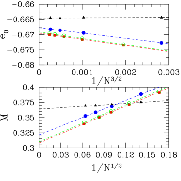
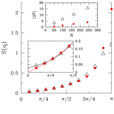
Figure 3: Upper left panel: energy per site as a function of cluster size $N$, showing exact results (full squares), variational results obtained by considering Eqs. (46) and (48) with the spin Jastrow factor (49) (full circles), and variational results obtained with Eqs. (46) and (47) (full triangles). The results obtained by optimizing the pairing function $f_{R,R^{\prime}}^{bos}$ of the bosonic representation, described in section 0.4, are also shown (empty circles) sandvik4 . Lower left panel: staggered magnetization with the same notation as in the upper panel. Right panel: static structure factor $S(q)$ for a cluster with $N=242$ (tilted by $45^{\circ}$): variational results for the state of Eqs. (46) and (48) with a long-range Jastrow factor (full dots) and for the wave function of Eqs. (46) and (47) with a nearest-neighbor Jastrow factor (empty triangles). Lower inset: detail at small momenta. Upper inset: square of total spin $\langle S^{2}\rangle$ as a function of $N$ for the two states, using the same symbols.

We move now to consider the two-dimensional case, starting with the unfrustrated model ($J_{2}=0$), for which exact results can be obtained by Monte Carlo methods reger ; sandvik3 ; calandra . In the thermodynamic limit, the ground state is antiferromagnetically ordered with a staggered magnetization reduced to approximately $60\%$ of its classical value, namely $M\simeq 0.307$ sandvik3 ; calandra . This quantity can be obtained both from the spin-spin correlations at the largest distances and from the spin structure factor $S(q)$ at $q=(\pi,\pi)$. In the following, we will consider the former definition and will calculate the isotropic correlations $\langle{\bf S}_{R}\cdot{\bf S}_{R^{\prime}}\rangle$, because this quantity is known to have smaller finite-size effects reger ; sandvik3 . For the unfrustrated case, the best wave function has $\epsilon_{k}=-2t(\cos k_{x}+\cos k_{y})$ and a pairing function with $d_{x^{2}-y^{2}}$ symmetry, $\Delta^{x^{2}-y^{2}}_{k}=\Delta_{1}(\cos k_{x}-\cos k_{y})$ (possibly also with higher harmonics connecting opposite sublattices). The quantity $\Delta_{AF}$ in Eq. (48) has a finite value and the spin Jastrow factor (49) has an important role.

Figure 3 shows the comparison of the variational calculations with the exact results, which are available for rather large system sizes. In the unfrustrated case, the bosonic representation is considerably better than the fermionic one: the accuracy in the energy is around $0.06\%$ and the sublattice magnetization is also very close to the exact value lou ; sandvik4 . However, the fermionic state defined by Eqs. (46) and (48), in combination with the spin Jastrow factor, also provides a very good approximation to the exact results (energy per site and staggered magnetization), whereas the wave function defined by Eqs. (46) and (47) is rather inaccurate. It should be emphasized that when the Jastrow factor is included, the slopes of the finite-size scaling functions are also remarkably similar to the exact ones, both for the energy per site $e_{0}$ and for the magnetization $M$. This implies that the pBCS wave function provides an accurate estimate of the spin velocity $c$, of the transverse susceptibility $\chi_{\perp}$, and as a consequence of the spin stiffness, $\rho_{s}=c^{2}\chi_{\perp}$. By contrast, the wave function without the Jastrow factor leads to a vanishing spin velocity. We note that in this case the staggered magnetization $M\simeq 0.365$ is also overestimated in the thermodynamic limit.

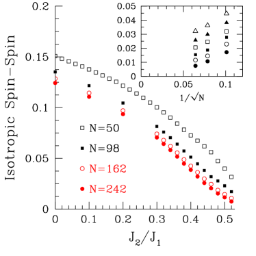
Figure 4: Left panel: spin-spin correlations at the largest distances as a function of the ratio $J_{2}/J_{1}$ for different cluster sizes $N$. Inset: finite-size scaling for $J_{2}/J_{1}=0.42$ (empty triangles), $0.44$ (full triangles), $0.46$ (empty squares), $0.48$ (full squares), $0.50$ (empty circles), and $0.52$ (full circles). Right panel: spin-spin correlations at the largest distances for $J_{2}/J_{1}>0.7$.

The functional form of the Jastrow factor at long ranges, which can be obtained by minimizing the energy, is necessary to reproduce correctly the small-$q$ behavior of the spin-structure factor $S(q)$, mimicking the Goldstone modes typical of a broken continuous symmetry manousakis . Indeed, it is clear from Fig. 3 that only with a long-range spin Jastrow factor it is possible to obtain $S(q)\sim|q|$ for small momenta, consistent with a gapless spin spectrum. By contrast, with a short-range spin Jastrow factor (for example with a nearest-neighbor term), $S(q)\sim{\rm const}$ for small $q$, which is clearly not correct manousakis . Finally, it should be emphasized that the combined effects of the magnetic order parameter $\Delta_{AF}$ and the spin Jastrow factor give rise to an almost singlet wave function, strongly reducing the value of $\langle S^{2}\rangle$ compared to the case without a long-range Jastrow term (see Fig. 3).

On increasing the value of the frustrating superexchange $J_{2}$, the Monte Carlo method is no longer numerically exact because of the sign problem, whereas the variational approach remains easy to apply. In Fig. 4, we present the results for the spin-spin correlations at the maximum accessible distances for $J_{2}/J_{1}\leq 0.52$. It is interesting to note that when $J_{2}/J_{1}>0.4$, a sizable energy gain may be obtained by adding a finite pairing connecting pairs on the same sublattice with $d_{xy}$ symmetry, namely $\Delta_{k}=\Delta^{x^{2}-y^{2}}_{k}+\Delta^{xy}_{k}$ capriotti . The mean-field order parameter $\Delta_{AF}$ remains finite up to $J_{2}/J_{1}\sim 0.5$, whereas for $J_{2}/J_{1}>0.5$ it goes to zero in the thermodynamic limit. Because the Jastrow factor is not expected to destroy the long-range magnetic order, the variational technique predicts that antiferromagnetism survives up to higher frustration ratios than expected doucot , similar to the outcome of a Schwinger boson calculation mila . The magnetization also remains finite, albeit very small, up to $J_{2}/J_{1}=0.5$ (see Fig. 4). We remark here that by using the bosonic RVB state, Beach argued that the Marshall-Peierls sign rule may hold over a rather large range of frustration, namely up to $J_{2}/J_{1}=0.418$, also implying a finite staggered magnetic moment beach . In this approach, if one assumes a continuous transition from the ordered to the disordered phase, the critical value is found to be $J_{2}/J_{1}=0.447$, larger than the value of Ref. doucot and much closer to our variational prediction. We note in this context that recent results obtained by coupled cluster methods are also similar, i.e., $J_{2}/J_{1}\sim 0.45$ for a continuous phase transition between a Néel ordered state and a quantum paramagnet darradi .

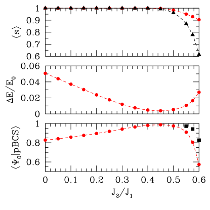
Figure 5: Comparison between exact and variational results on a $6\times 6$ lattice. The pBCS wave function has $\Delta_{AF}=0$ and no Jastrow factor. Upper panel: average sign $\langle s\rangle$ of Eq. (57) (full circles); the Marshall-Peierls sign, $\langle s\rangle_{MA}=\sum_{x}|\langle x|\Psi_{0}\rangle|^{2}{\rm sign}\left\{\langle x|\Psi_{0}\rangle(-1)^{N_{\uparrow}(x)}\right\}$, is also shown (full triangles). Middle panel: accuracy of the ground-state energy, $\Delta E/E_{0}=(E_{0}-E_{pBCS})/E_{0}$, where $E_{0}$ and $E_{pBCS}$ are the exact and the variational energies, respectively. Lower panel: overlap between the exact $|\Psi_{0}\rangle$ and variational $|pBCS\rangle$ states (full circles). The norm of the projection of the variational state onto the subspace spanned by the two lowest-energy states in the same symmetry sector is also shown (full squares) close to the first-order transition to the collinear state.

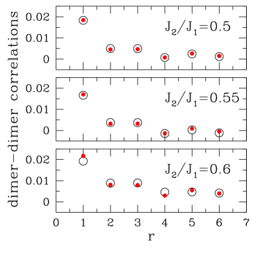
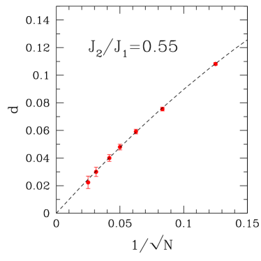
Figure 6: Left panels: dimer-dimer correlations as a function of the Manhattan distance for exact (empty circles) and variational (full dots) calculations on a $6\times 6$ cluster. Right panel: finite-size scaling of the dimer order parameter for $J_{2}/J_{1}=0.55$.

Table 1: Energies per site for a $6\times 6$ lattice. $E_{pBCS}$ obtained from the pBCS wave function (with $\Delta_{AF}=0$ and no Jastrow factor), $E_{LR-RVB}$ from the long-range bosonic RVB state, optimizing just one parameter using the master-equation method beach2 , and $E_{SR-RVB}$ obtained by diagonalizing the $J_{1}{-}J_{2}$ model in the nearest-neighbor valence-bond basis mambrini2 . The exact results $E_{0}$ are also reported.

$J_{2}/J_{1}$	$E_{SR-RVB}$	$E_{LR-RVB}$	$E_{pBCS}$	$E_{0}$
0.30	-0.54982	-0.5629(5)	-0.55569(2)	-0.56246
0.35	-0.53615	-0.5454(5)	-0.54134(1)	-0.54548
0.40	-0.52261	-0.5289(5)	-0.52717(1)	-0.52974
0.45	-0.50927		-0.51365(1)	-0.51566
0.50	-0.49622		-0.50107(1)	-0.50381
0.55	-0.48364		-0.48991(1)	-0.49518
0.60	-0.47191		-0.47983(2)	-0.49324

In the regime of large $J_{2}/J_{1}$ (i.e., $J_{2}/J_{1}>0.65$), collinear order with pitch vectors $Q=(0,\pi)$ and $Q=(\pi,0)$ is expected. The pBCS wave function is also able to describe this phase through a different choice for the bare electron dispersion, namely $\epsilon_{k}=-2t^{\prime}[\cos(k_{x}+k_{y})+\cos(k_{x}-k_{y})]$ and $\Delta_{k}=\Delta_{1}\cos k_{x}+\Delta_{2}[\cos(k_{x}+k_{y})-\cos(k_{x}-k_{y})]$, with $\Delta_{1}\to 0$ for $J_{1}/J_{2}\to 0$. Further, the antiferromagnetic wave vector $Q$ in Eq. (48) is $Q=(\pi,0)$. The variational wave function breaks the reflection symmetry of the lattice and, in finite systems, its energy can be lowered by projecting the state onto a subspace of definite symmetry. The results for the spin-spin correlations are shown in Fig. 4. By decreasing the value of $J_{2}/J_{1}$, we find clear evidence of a first-order phase transition, in agreement with previous calculations using different approaches singh2 ; sushkov .

For $0.5<J_{2}/J_{1}<0.65$, the best variational wave function has no magnetic order ($\Delta_{AF}=0$ and no Jastrow factor) and the BCS Hamiltonian has $\epsilon_{k}=-2t(\cos k_{x}+\cos k_{y})$ and $\Delta_{k}=\Delta^{x^{2}-y^{2}}_{k}+\Delta^{xy}_{k}$, where $\Delta^{x^{2}-y^{2}}_{k}$ connects pairs on opposite sublattices while $\Delta^{xy}_{k}$ is for same sublattice. With this specific electron pairing, the signs of the wave function are different from those predicted by the Marshall-Peierls rule and are much more similar to the exact ones. We define

$$\langle s\rangle=\sum_{x}|\langle x|pBCS\rangle|^{2}{\rm sign}\left\{\langle x|pBCS\rangle\langle x|\Psi_{0}\rangle\right\},$$ (57)

where $|pBCS\rangle$ and $|\Psi_{0}\rangle$ are the variational and the exact states, respectively. This quantity is shown in Fig. 5, together with the Marshall-Peierls sign, for a $6\times 6$ lattice. The variational energy, the very large overlap with the exact ground state, and the dimer-dimer correlations shown in Figs. 5 and 6, all reflect the extremely high accuracy of this state in the strongly frustrated regime. On small clusters, the overlap between the variational wave function and the ground state deteriorates for $J_{2}/J_{1}>0.55$. This may be a consequence of the proximity to the first order transition, which marks the onset of collinear magnetic order, and implies a mixing of the two finite-size ground states corresponding to the coexisting phases.

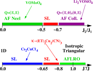
Figure 7: Upper panel: phase diagram of the $J_{1}{-}J_{2}$ model on the square lattice, as deduced from the variational approach. Lower panel: phase diagram of the anisotropic triangular lattice from Ref. yunoki . The approximate locations of some relevant materials are indicated by the arrows.

In Table 1, we report the comparison between the energies of the non-magnetic pBCS wave function and two bosonic RVB states. The first is obtained by a full diagonalization of the $J_{1}{-}J_{2}$ model in the nearest-neighbor valence-bond basis, namely by optimizing all the amplitudes of the independent valence-bond configurations without assuming the particular factorized form of Eq. (42) mambrini2 . Although this wave function contains a very large number of free parameters, its energy is always higher than that obtained from the pBCS state, showing the importance of having long-range valence bonds. A further drawback of this approach is that it is not possible to perform calculations on large system sizes, the upper limit being $N\sim 40$. The second RVB state is obtained by considering long-range valence bonds, with their amplitudes given by Eq. (42) and optimized by using the master-equation scheme beach2 . While this wave function is almost exact in the weakly frustrated regime, its accuracy deteriorates on raising the frustrating interaction, and for $J_{2}/J_{1}>0.425$ the minus-sign problem precludes the possibility of reliable results. On the other hand, the pBCS state (without antiferromagnetic order or the Jastrow term) becomes more and more accurate on approaching the disordered region. Remarkably, for $J_{2}/J_{1}=0.4$, the energy per site in the thermodynamic limit obtained with the long-range bosonic wave function is $E/J_{1}=-0.5208(2)$, which is very close to and only slightly higher than that obtained from the fermionic representation, $E/J_{1}=-0.5219(1)$.

In the disordered phase, the pBCS wave function does not break any lattice symmetries (section 0.3) and does not show any tendency towards a dimerization. Indeed, the dimer order parameter $d$ (calculated from the correlations at the longest distances) vanishes in the thermodynamic limit, as shown in Fig. 6, implying a true spin-liquid phase in this regime of frustration. This fact is in agreement with DMRG calculations on ladders with odd numbers of legs, suggesting a vanishing spin gap for all values of $J_{2}/J_{1}$ capriotti2 , in sharp contrast to the dimerized phase, which has a finite triplet gap.

Taking together all of the above results, it is possible to draw the (zero-temperature) phase diagram generated by the variational approach, and this is shown in Fig. 7.

We conclude by considering the important issue of the low-energy spectrum. In two dimensions, it has been argued that the ground state of a spin-1/2 system is either degenerate or it sustains gapless excitations hastings , in analogy to the one-dimensional case lsm . In Ref. ivanov , it has been shown that the wave function with both $d_{x^{2}-y^{2}}$ and $d_{xy}$ parameters could have topological order. In fact, by changing the boundary conditions of the BCS Hamiltonian, it should be possible to obtain four different projected states which in the thermodynamic limit are degenerate and orthogonal but, however, not connected by any local spin operator. In this respect, it has been argued more recently that a topological degeneracy may be related to the signs of the wave function and cannot be obtained for states satisfying the Marshall-Peierls rule li .

In the spin-liquid regime, the simultaneous presence of $\Delta^{x^{2}-y^{2}}_{k}$ and $\Delta^{xy}_{k}$ could shift the gapless modes of the unprojected BCS spectrum $E_{k}$ from $(\pm\pi/2,\pm\pi/2)$ to incommensurate $k$-points along the Fermi surface determined by $\epsilon_{k}=0$. However, we have demonstrated recently that a particular $\Delta^{xy}_{k}$ pairing, $\Delta^{xy}_{k}\propto\sin(2k_{x})\sin(2k_{y})$, may be imposed, in order to fix the nodes at the commensurate points $(\pm\pi/2,\pm\pi/2)$, without paying an additional energy penalty. Once $E_{k}$ is connected to the true spin excitations, a gapless spectrum is also expected. At present, within a pure variational technique, it is not possible to assess the possibility of incommensurate, gapless spin excitations being present. An even more challenging problem is to understand if the topological states could survive at all in the presence of a gapless spectrum.

0.7 Other frustrated lattices

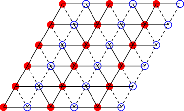
Figure 8: Nearest-neighbor pairing function consistent with the sign convention of the short-range RVB state in the triangular lattice: solid (dashed) lines represent positive (negative) values. Note that the unit cell contains two sites, indicated by empty and full circles.

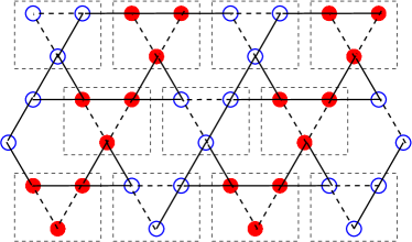
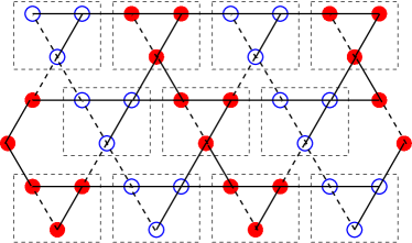
Figure 9: Left panel: signs of the real hopping terms $\chi_{R,R^{\prime}}$ of the U(1) Dirac spin liquid on the kagome lattice [Eq. (59)] palee . Solid (dashed) lines represent positive (negative) values. The unit cell contains six sites (three empty and three full circles inside the boxes). Right panel: nearest-neighbor pairing function consistent with the sign convention of the short-range RVB state in the kagome lattice: solid (dashed) lines represent positive (negative) values. The unit cell also contains six sites in this case.

In this last section, we provide a brief overview of related variational studies performed for other lattice structures. In particular, we discuss in some detail the symmetries of the variational wave function on the anisotropic triangular lattice, considered in Ref. yunoki . In this case, one-dimensional chains with antiferromagnetic interaction $J$ are coupled together by a superexchange $J^{\prime}$, such that by varying the ratio $J^{\prime}/J$, the system interpolates between decoupled chains ($J^{\prime}=0$) and the isotropic triangular lattice ($J^{\prime}=J$); the square lattice can also be described in the limit of $J=0$. The case with $J^{\prime}<J$ may be relevant for describing the low-temperature behavior of ${\rm Cs_{2}CuCl_{4}}$ coldea , whereas $J^{\prime}\sim J$ may be pertinent to the insulating regime of some organic materials, such as $\kappa-{\rm(ET)_{2}Cu_{2}(CN)_{3}}$ kanoda .

In Ref. yunoki , it has been shown that very accurate variational wave functions can be constructed, providing evidence in favor of two different spin-liquid phases, a gapped one close to the isotropic point and a gapless one close to the one-dimensional regime, see Fig. 7. We focus our attention on the isotropic point. In this case, a natural variational ansatz is the bosonic short-range RVB state of Eq. (42) sindzingre . Exact numerical calculations for the $6\times 6$ isotropic model have shown that the overlap between the short-range RVB wave function and the ground state is very large, $|\langle RVB|\Psi_{0}\rangle|^{2}=0.891$, and also that the average sign $\langle s\rangle=\sum_{x}|\langle x|\Psi_{0}\rangle|^{2}{\rm sign}\left\{\langle x|\Psi_{0}\rangle\langle x|RVB\rangle\right\}=0.971$ yunoki is very close to its maximal value, $\langle s\rangle=1$. We note that both the values of the overlap and of the average sign are much better than those obtained by a wave function that describes a magnetically ordered state, despite the smaller number of variational parameters capriottitri . Although the short-range RVB state is a very good variational ansatz, the bosonic representation of this state is rather difficult to handle in large clusters. Its systematic improvement by the inclusion of long-range valence bonds leads to a very severe sign problem, even at the variational level sindzingre . In this respect, following the rules discussed in section 0.4, it is possible to obtain a fermionic representation of the short-range RVB state. The signs of the pairing function $f_{R,R^{\prime}}$ are given in Fig. 8 for open boundary conditions. Remarkably, this particular pattern leads to a $2\times 1$ unit cell, which cannot be eliminated by using local SU(2) transformations of the type discussed in section 0.2. The variational RVB wave function is obtained by projecting the ground state of the BCS Hamiltonian, with a particular choice of the couplings: the only nonzero parameters are the chemical potential $\mu$ and the nearest-neighbor singlet gap $\Delta_{R,R^{\prime}}$, in the limit $-\mu\gg|\Delta_{R,R^{\prime}}|$ (so that the pairing function is proportional to the superconducting gap). The amplitude of the gap $|\Delta_{R,R^{\prime}}|=\Delta$ is uniform, while the appropriate phases are shown in Fig. 8. The BCS Hamiltonian is defined on a $2\times 1$ unit cell and, therefore, is not translationally invariant. Despite the fact that it is invariant under an elementary translation ${\cal T}_{2}$ in the $\tau_{2}=(1/2,\sqrt{3}/2)$ direction, it is not invariant under an elementary translation ${\cal T}_{1}$ in the $\tau_{1}=(1,0)$ direction. Nevertheless, this symmetry is recovered after the projection $P_{G}$, making $|pBCS\rangle$ translationally invariant. Indeed, one can combine the translation operation ${\cal T}_{1}$ with the SU(2) gauge transformation

$$c^{{\dagger}}_{R,\sigma}\to-c^{{\dagger}}_{R,\sigma}$$ (58)

for $R=m_{1}\tau_{1}+m_{2}\tau_{2}$ with $m_{2}$ odd. Under the composite application of the transformations ${\cal T}_{1}$ and (58), the projected BCS wave function does not change. Because the gauge transformation acts as an identity in the physical Hilbert space with singly occupied sites, $|pBCS\rangle$ is translationally invariant.

Table 2: Variational energy estimated in the thermodynamic limit for the antiferromagnetic Heisenberg model on the isotropic triangular lattice ($J^{\prime}=J$).

wave function	$E/J$
short-range RVB	$-0.5123(1)$
RVB with $\mu=0$	$-0.5291(1)$
best RVB yunoki	$-0.5357(1)$
BCS+Néel weber	$-0.532(1)$

Through this more convenient representation of the short-range RVB state by the pBCS wave function, it is possible to calculate various physical quantities using the standard variational Monte Carlo method. One example is the very accurate estimate of the variational energy per site in the thermodynamic limit, $E/J=-0.5123(1)$ yunoki . Another important advantage of the fermionic representation is that it is easy to improve the variational ansatz in a systematic way. The variational energy can be improved significantly by simply changing the chemical potential $\mu$ from a large negative value to zero, see Table 2. We note that in this case $|pBCS\rangle$ is equivalent to a Gutzwiller-projected free fermion state with nearest-neighbor hoppings defined in a $2\times 1$ unit cell, because, through the SU(2) transformation of Eq (24), the off-diagonal pairing terms are transformed into kinetic terms. Further, the BCS Hamiltonian may be extended readily to include long-range valence bonds by the simple addition of nonzero $\Delta_{R,R^{\prime}}$ or $t_{R,R^{\prime}}$ terms. It is interesting to note that, within this approach, it is possible to obtain a variational energy $E/J=-0.5357(1)$ lower than that obtained by starting from a magnetically ordered state and considered in Ref. weber , see Table 2.

Finally, projected states have been also used to describe the ground state of the Heisenberg Hamiltonian on the kagome lattice palee ; palee2 . In this case, different possibilities for the mean-field Hamiltonian have been considered, with no BCS pairing but with non-trivial fluxes through the triangles and the hexagons of which the kagome structure is composed. In particular, the best variational state in this class can be found by taking

$${\cal H}_{MF}=-\sum_{\langle R,R^{\prime}\rangle,\sigma}\chi_{R,R^{\prime}}c^{\dagger}_{R,\sigma}c_{R^{\prime},\sigma}+H.c.,$$ (59)

with all the hoppings $\chi_{R,R^{\prime}}$ having the same magnitude and producing a zero flux through the triangles and $\pi$ flux through the hexagons. One may fix a particular gauge in which all $\chi_{R,R^{\prime}}$ are real, see Fig. 9. In this gauge, the mean-field spectrum has Dirac nodes at $k=(0,\pm\pi/\sqrt{3})$, and the variational state describes a U(1) Dirac spin liquid. Remarkably, this state should be stable against dimerization (i.e., it has a lower energy than simple valence-bond solids), in contrast to mean-field results hastings2 . Another competing mean-field state hastings2 , which is obtained by giving the fermions chiral masses and is characterized by a broken time-reversal symmetry (with $\theta$ flux through triangles and $\pi-\theta$ flux through hexagons), is also found to have a higher energy than the pure spin-liquid state. In this context, it would be valuable to compare the wave function proposed in Ref. palee with the systematic improvement of the short-range RVB state which has a simple fermionic representation (see Fig. 9).

0.8 Conclusions

In summary, we have shown that projected wave functions containing both electronic pairing and magnetism provide an extremely powerful tool to study highly frustrated magnetic materials. In particular, these pBCS states may describe all known phases in one-dimensional systems, giving very accurate descriptions when compared to state-of-the-art DMRG calculations. Most importantly, variational wave functions may be easily generalized to treat higher dimensional systems: here we have presented in detail the case of the two-dimensional $J_{1}{-}J_{2}$ model, as well as some examples of other frustrated lattices which have been considered in the recent past.

The great advantage of this variational approach in comparison with other methods, such as DMRG, is that it can offer a transparent description of the ground-state wave function. Furthermore, the possibility of giving a physical interpretation of the unprojected BCS spectrum $E_{k}$, which is expected to be directly related to the true spin excitations, is very appealing. We demonstrated that this correspondence works very well in one dimension, both for gapless and for dimerized phases. In two dimensions, the situation is more complicated and we close by expressing the hope that future investigations may shed further light one the fascinating world of the low-energy properties of disordered magnetic systems.

References

- (1) J.R. Schrieffer, “Theory of Superconductivity”, Addison Wesley (1964).
- (2) R.B. Laughlin, Phys. Rev. Lett. 50, 1395 (1983).
- (3) P.W. Anderson, Mater. Res. Bull 8, 153 (1973); P. Fazekas and P.W. Anderson, Philos. Mag. 30, 423 (1974).
- (4) For a review see G. Misguich and C. Lhuillier, in “Frustrated Spin Models”, Ed. H. T. Diep, World Scientific, New Jersey (2004); see also G. Misguich in this volume.
- (5) G. Castilla, S. Chakravarty, and V.J. Emery, Phys. Rev. Lett. 75, 1823 (1995).
- (6) R. Melzi, P. Carretta, A. Lascialfari, M. Mambrini, M. Troyer, P. Millet, and F. Mila, Phys. Rev. Lett. 85, 1318 (2000).
- (7) P. Carretta, N. Papinutto, C. B. Azzoni, M. C. Mozzati, E. Pavarini, S. Gonthier, and P. Millet, Phys. Rev. B 66, 094420 (2002).
- (8) S.R. White and I. Affleck, Phys. Rev. B 54, 9862 (1996).
- (9) S. Eggert, Phys. Rev. B 54, 9612 (1996).
- (10) C.K. Majumdar and D.K. Ghosh, J. Math. Phys. 10, 1388, (1969).
- (11) C.K. Majumdar and D.K. Ghosh, J. Math. Phys. 10, 1399 (1969).
- (12) P. Chandra and B. Doucot, Phys. Rev. B 38, 9335 (1988).
- (13) E. Dagotto and A. Moreo, Phys. Rev. Lett. 63, 2148 (1989).
- (14) R.R.P. Singh and R. Narayanan, Phys. Rev. Lett. 65, 1072 (1990).
- (15) J. Schulz, T.A. Ziman, and D. Poilblanc, J. Phys. I 6, 675 (1996).
- (16) M.P. Gelfand, R.R.P. Singh, and D.A. Huse, Phys. Rev. B 40, 10801 (1989).
- (17) R.R.P. Singh, Z. Weihong, C.J. Hamer, and J. Oitmaa, Phys. Rev. B 60, 7278 (1999).
- (18) V.N. Kotov, J. Oitmaa, O.P. Sushkov, and Z. Weihong, Phil. Mag. B 80, 1483 (2000).
- (19) O.P. Sushkov, J. Oitmaa, and Z. Weihong, Phys. Rev. B 63, 104420 (2001).
- (20) N. Read and S. Sachdev, Phys. Rev. Lett. 62, 1694 (1989).
- (21) M. Mambrini, A. Lauchli, D. Poilblanc, and F. Mila, Phys. Rev. B 74, 144422 (2006).
- (22) E. Lieb and D. Mattis, J. Math. Phys. 3, 749 (1962).
- (23) W. Marshall, Proc. R. Soc. London Ser. A 232, 48 (1955).
- (24) J. Richter, N.B. Ivanov, and K. Retzlaff, Europhys. Lett. 25, 545 (1994).
- (25) D.F.B. ten Haaf, H.J.M. van Bemmel, J.M.J. van Leeuwen, W. van Saarloos, and D.M. Ceperley, Phys. Rev. B 51, 13039 (1995).
- (26) P.W. Anderson, Science 235, 1196 (1987).
- (27) S. Liang, B. Doucot, and P.W. Anderson, Phys. Rev. Lett. 61, 365 (1988).
- (28) P. Sindzingre, P. Lecheminant, and C. Lhuillier, Phys. Rev. B 50, 3108 (1994).
- (29) F. Becca, L. Capriotti, A. Parola, and S. Sorella, Phys. Rev. B 76, 060401 (2007).
- (30) I. Affleck, Z. Zou, T. Hsu, and P.W. Anderson, Phys. Rev. B 38, 745 (1988).
- (31) F.-C. Zhang, C. Gros, T.M. Rice, and H. Shiba, Supercond. Sci. Technol. 36, 1 (1988).
- (32) X.-G. Wen, Phys. Rev. B 65, 165113 (2002).
- (33) F.D.M. Haldane, Phys. Rev. Lett. 60, 635 (1988).
- (34) J. Lou and A.W. Sandvik, Phys. Rev. B 76, 104432 (2007).
- (35) K.S.D. Beach and A.W. Sandvik, Nucl. Phys. B 750, 142 (2006).
- (36) A.W. Sandvik and K.S.D. Beach, arXiv:0704.1469.
- (37) K.S.D. Beach, arXiv:0709.3297.
- (38) B. Sutherland, Phys. Rev. B 37, 3786 (1988).
- (39) N. Read and B. Chakraborty, Phys. Rev. B 40, 7133 (1989).
- (40) P.W. Kasteleyn, J. Math. Phys. 4, 287 (1963).
- (41) C. Gros, Phys. Rev. B 42, 6835 (1990).
- (42) E. Manousakis, Rev. Mod. Phys. 63, 1 (1991).
- (43) F. Franjic and S. Sorella, Prog. Theor. Phys. 97, 399 (1997).
- (44) J.P. Bouchaud, A. Georges, and C. Lhuillier, J. Phys. (Paris) 49, 553 (1988).
- (45) S. Sorella, Phys. Rev. B 71, 241103 (2005).
- (46) C. Gros, Ann. of Phys. 189, 53 (1989).
- (47) I. Affleck, D. Gepner, H.J. Schulz, and T. Ziman, J. Phys. A 22, 511 (1989).
- (48) S. Sorella, L. Capriotti, F. Becca, and A. Parola, Phys. Rev. Lett. 91, 257005 (2003).
- (49) A. Parola, S. Sorella, F. Becca, and L. Capriotti, condmat/0502170.
- (50) J.D. Reger and A.P. Young, Phys. Rev. B 37, 5978 (1988).
- (51) A.W. Sandvik, Phys. Rev. B 56, 11678 (1997).
- (52) M. Calandra Buonaura and S. Sorella, Phys. Rev. B 57, 11446 (1998).
- (53) A.W. Sandvik, private communication.
- (54) L. Capriotti, F. Becca, A. Parola, and S. Sorella, Phys. Rev. Lett. 87, 097201 (2001).
- (55) F. Mila, D. Poilblanc, and C. Bruder, Phys. Rev. B 43, 7891 (1991).
- (56) R. Darradi, O. Derzhko, R. Zinke, J. Schulenburg, S.E. Krueger, and J. Richter, arXiv:0806.3825.
- (57) M. Mambrini, private communication.
- (58) K.S.D. Beach, private communication.
- (59) L. Capriotti, unpublished.
- (60) M.B. Hastings, Phys. Rev. B 69, 104431 (2004).
- (61) E.H. Lieb, T.D. Schultz, and D.C. Mattis, Ann. Phys. (N.Y.) 16, 407 (1961).
- (62) D.A. Ivanov and T. Senthil, Phys. Rev. B 66, 115111 (2002).
- (63) T. Li and H.-Y. Yang, Phys. Rev. B 75, 172502 (2007).
- (64) S. Yunoki and S. Sorella, Phys. Rev. B 74, 014408 (2006).
- (65) R. Coldea, D.A. Tennant, A.M. Tsvelik, and Z. Tylczynski, Phys. Rev. Lett. 86, 1335 (2001).
- (66) Y. Shimizu, K. Miyagawa, K. Kanoda, M. Maesato, and G. Saito, Phys. Rev. Lett. 91, 107001 (2003).
- (67) L. Capriotti, A.E. Trumper, and S. Sorella, Phys. Rev. Lett. 82, 3899 (1999).
- (68) C. Weber, A. Laeuchli, F. Mila, and T. Giamarchi, Phys. Rev. B 73, 014519 (2006).
- (69) Y. Ran, M. Hermele, P.A. Lee, and X.-G. Wen, Phys. Rev. Lett. 98, 117205 (2007).
- (70) M. Hermele, Y. Ran, P.A. Lee, and X.-G. Wen, Phys. Rev. B 77, 224413 (2008).
- (71) M.B. Hastings, Phys. Rev. B 63, 014413 (2000).