Is there evidence for field restructuring or decay in accreting magnetic white dwarfs?

Abstract

The evolution of the magnetic field of an accreting magnetic white dwarf with an initially dipolar field at the surface has been studied for non-spherical accretion under simplifying assumptions. Accretion on to the polar regions tends to advect the field toward the stellar equator which is then buried. This tendency is countered by Ohmic diffusion and magneto-hydrodynamic instabilities. It is argued that if matter is accreted at a rate of $\dot{M}_{\rm crit}\sim 10^{16}$ g s^-1 and the total mass accreted exceeds a critical value $\Delta M_{\rm crit}\sim 0.1-0.2M_{\odot}$, the field may be expected to be restructured, and the polar field to be reduced reaching a minimum value of $\sim 10^{3}$ G (the “bottom field”) independently of the initial field strength. Below this critical accretion rate, the field diffuses faster than it can be advected, and accretion has little effect on field strength and structure.

In polars, where the magnetic field strength ($\sim 10^{7}-10^{8}$ G) is strong enough to lock the magnetic white dwarf into synchronous rotation with the orbit and a disc does not form, magnetic braking is severely curtailed as the stellar wind from the secondary becomes trapped in the combined magnetosphere of the two stars. The mass transfer rate in such systems is typically $\mbox{$\,\stackrel{{\scriptstyle\scriptstyle<}}{{\scriptstyle\sim}}\,$}10^{16}$ g s^-1, and field restructuring is not expected. In systems with fields not strong enough to achieve synchronism and where accretion occurs via a truncated disc (the intermediate polars), normal magnetic braking may be expected. The mass transfer rates are then typically $\mbox{$\,\stackrel{{\scriptstyle\scriptstyle>}}{{\scriptstyle\sim}}\,$}10^{16}$ g s^-1 above the $2-3$ hour Cataclysmic Variable period gap, and thus a significant reduction of the polar field strength could occur if such a system accumulates the required critical mass $M_{\rm crit}$. However, due to mass loss during nova eruptions, only a small fraction of such systems (those that first come into contact at long orbital periods) may accumulate sufficient mass to reach the bottom field configuration. We argue that the observed properties of the Magnetic Cataclysmic Variables (MCVs) can generally be explained by a model where the field is at most only partially restructured due to accretion. If there are systems that have reached the bottom field, they may be found among the dwarf novae, and be expected to exhibit quasi periodic oscillations.

1 Introduction

In the Magnetic Cataclysmic Variables (MCVs) which comprise some $25$% of the Cataclysmic Variables (CVs), there is direct or indirect evidence for a magnetic field that influences the accretion flow on to the white dwarf. MCVs tend to fall into two distinct classes: the AM Herculis-type variables (or polars) and the intermediate polars (IPs) (see Warner 1995 for a comprehensive review; Patterson 1994; Wood et al. 2000; Wickramasinghe and Ferrario 2000, hereafter WF00).

In the vast majority of the polars, the magnetic field of the white dwarf is strong enough to magnetically lock it into synchronous rotation with the orbital period through magnetic interaction with the secondary star. Thus, in polars the spin period $P_{\rm s}$ equals the orbital period $P_{\rm orb}$. Only a handful of polars are slightly asynchronous ($P_{s}/P_{\rm orb}\sim 0.99$), likely due to recent nova events during which synchronism was broken. In polars, accretion occurs directly on to the magnetic white dwarf (MWD) without the formation of an accretion disc. The magnetic fields in polars are well determined through the observation of cyclotron and Zeeman features, and are found to be in the range $7-230$ MG (WF00).

The IPs are characterised by the presence of asynchronously rotating white dwarfs with $P_{s}/P_{\rm orb}\sim 0.01-0.9$. In these systems, accretion occurs via a truncated accretion disc and magnetically confined accretion curtains (e.g. Ferrario & Wickramasinghe 1993; Ferrario, Wickramasinghe & King 1993). A direct field measurement is only available for one IP: V405 Aurigae for which low-resolution circular spectropolarimetry has revealed the presence of cyclotron harmonics corresponding to a field of 31.5 MG (Piirola et al. 2008) which is in the range of fields found in the polars. However, as a class, IPs tend to be at the lower end ($\sim 5-20$ MG) of the field distribution in polars, as it is inferred by the circular polarization survey of IPs conducted by Butters et al. (2009). Fields estimated on the assumption that the white dwarf is in spin equilibrium with an accretion disc generally confirms this expectation (e.g. Norton, Wynn & Somerscales 2004). The field distributions of the polar and the IPs with fields determined either directly (in the case of polars), or with the assumption of spin equilibrium and/or broadband circular polarization measurements (in the case of IPs) are shown in Figure 1.

Figure 1: Magnetic field distribution of the polars (solid histogram), and the intermediate polars (shaded histogram). The IP magnetic fields are calculated by assuming that these systems are at their equilibrium spin period (Norton et al. 2004), so the fields are not measured directly like in polars. The dashed histogram shows the distribution of fields in the high field isolated magnetic white dwarfs.

There are some parallels and differences with the observed properties of the isolated Magnetic White Dwarfs (MWDs) which fall into two disjoint groups: the high field magnetic white dwarfs (HFMWDs) with fields in the range $10^{6}-10^{9}$ G, and the low field magnetic white dwarfs (LFMWDs) with fields $<10^{5}$ G (see WF00 and Wickramasinghe & Ferrario 2009 for a comprehensive review). The HFMWDs comprise some $12-15$% of all WDs detected in volume-limited surveys, while the LFMWDs form a group that is at least as numerous. The field distribution of the isolated HFMWDs is compared with that of the MCVs and is also shown in Figure 1. Although it is this group that is most likely to be associated with the MCVs, we note that there are distinct differences in the two distributions. The peak of the distribution for isolated HFMWDs occurs at $\sim\times 10^{7}$ G compared to $3\times 10^{7}$ for the MCVs. Furthermore, very high magnetic field systems ($10^{8}-10^{9}$)are not as well represented among the MCVs.

The magnetic properties of the isolated LFMWDs are less well established due to current limitations of measuring fields $\mbox{$\,\stackrel{{\scriptstyle\scriptstyle<}}{{\scriptstyle\sim}}\,$}10^{3}$ G. It is possible that all WDs are magnetic at some level and thus belong to the LFMWD group or it could be that most stars are essentially non magnetic. The LFMWDs are likely to be associated with the vast majority of the CVs that shows no direct evidence for coherent pulsations at the spin period of the white dwarf as expected if there is no magnetically channeled accretion on to the surface of the white dwarf. On the other hand, the study of Quasi-Periodic Oscillations (QPO) has indicated the possible presence of weak magnetic fields in some dwarf novae (e.g. Warner & Woudt 2002, 2008; Warner & Pretorius 2008).

The differences between the observed field distributions of the HFMWDs and MCVs may be due to observational selection effects or be caused by accretion which affects the surface magnetic field of the white dwarf. Isolated HFMWDs show no evidence of field decay on the time scale of the age of the galactic disc and these conclusions are generally consistent with theoretical estimates of time scales for free Ohmic decay of the dipolar mode. On the other hand, Cumming (2002, 2003, 2004) calculated the Ohmic decay modes for spherically accreting white dwarfs with a liquid interior allowing for compressional heating, and found Ohmic decay time scales of several billion years, comparable to the orbital evolutionary time scales of typical CVs. These calculations appear to suggest that field decay may play a role in our understanding of the observed properties of MCVs. However, it is unclear whether the assumption of spherical accretion is applicable to polars and IPs where accretion occurs via funnels onto magnetic polar caps.

In this paper, we ask the question whether the observations of IPs and Polars can be used to distinguish between the following three possibilities; (i) accretion induces a a net decrease in polar field strength and changes the field structure, (ii) accretion screens the field during phases of accretion but the field subsequently re-emerges to almost the original value when accretion ceases, or (iii) that accretion has little or no effect on the field strength and structure. Our study is based on a model of non-spherical accretion on to an initially dipolar magnetic field which was first developed for accreting neutron stars. Here, we extend these calculations to conditions appropriate to accreting white dwarfs. The model predicts that the magnetic polar cap widens as material is accreted with the field being advected towards the equatorial regions by the ensuing hydromagnetic flow (e.g., Romani 1990; Konar & Choudhury 2004; Payne & Melatos 2004; Zhang & Kojima 2006, hereafter ZK06). In the idealised case where Ohmic diffusion or MHD instabilities are assumed unimportant, the polar field reaches an asymptotic value (the so-called “bottom field”) as the equatorial field becomes fully submerged by the advected matter. One of the interpretations of the observed properties of neutron stars in the Low Mass X-ray Binaries (LMXBs) and the binary millisecond pulsars (BMSPs) is that such a bottom field has indeed been reached at a value of $\sim 10^{8}$ G (Wijnands & van der Klis 1998).

The paper is organized as follows. We describe the basic model in section 2.1, where we present and discuss the equations and solutions for the evolution of the polar field of the white dwarf in the case where diffusive effects or MHD instabilities are considered unimportant. The expected time scales for Ohmic diffusion and advection for conditions appropriate to accreting white dwarfs are discussed in section 2.2. The application to the MCVs is presented in section 3 where we discuss the various accretion regimes and the possible evidence for field restructuring and decline. Finally, our main conclusions are summarized in section 4.

2 The basic field advection model

2.1 Advection of polar magnetic zone

ZK06 developed a simple analytical model which encapsulates the basic physics of non-spherical accretion onto a magnetised neutron star with a centred dipolar field. On this model, as matter accretes along dipolar field lines onto the polar cap regions, the accreted matter moves both downwards into the deeper layers of the star, and in a perpendicular direction dragging the field lines with the flow towards the equatorial regions. The net effect is an increase in the width of the polar cap region which yields a decrease in the polar field strength $B$.

Following ZK06, we assume that as accretion proceeds, and the polar field $B$ decreases, the magnetospheric radius $R_{\rm M}$ continues to be given by the standard expression (Ghosh & Lamb 1979) for a dipolar magnetic field

$$R_{\rm M}=\phi R_{\rm A}=1.2\times 10^{11}({\rm cm})\phi\dot{M}^{-2/7}_{\rm 16}B_{7}^{4/7}R_{9}^{12/7}m^{-1/7}\,\,\,$$ (1)

where $R_{\rm A}$ is the spherical Alfven radius, and $\phi$ is a parameter which is estimated to be $\sim 0.5$ for disc accretion, but is model dependent (e.g. Li & Wang 1999). Further, $m=M/M_{\odot}$ is the white dwarf mass $M$ in units of solar masses, $R_{9}$ is the white dwarf radius in units of $10^{9}$ cm, $\dot{M}_{16}$ and $B_{7}$ are the accretion rate in units of $10^{16}$ g s^-1 and field in units of $10^{7}$ G, respectively. The bottom field $B_{\rm f}$ is reached when the magnetospheric radius $R_{\rm M}=R$, that is,

$$B_{{\rm f}}=2.8\times 10^{3}\,(G)\,\dot{M}_{16}^{1/2}m^{1/4}R^{-5/4}_{9}\phi^{-7/4}\,.$$ (2)

In the ZK06 model, the approach to the bottom field state is described by assuming that the motion that drags and restructures the field occurs in the regions of the star that are built up by accreted matter. It is further assumed that when the mass of this layer exceeds a critical value $\Delta M_{\rm crit}$, the accreted matter becomes incorporated into the interior of the star, and does not partake in further restructuring of the field. These assumptions, combined with the equations of continuity and magnetic flux conservation, lead to the following equation for the polar field $B$ in terms of the initial polar field $B_{o}$ before accretion, and the amount of mass $\Delta M$ accreted

$$B=\frac{B_{{\rm f}}}{\{1-\left[C/\exp(y)-1\right]^{2}\}^{7/4}}\,,$$ (3)

where $y=\displaystyle{\frac{2\xi\Delta M}{7\Delta M_{\rm crit}}}$, $\Delta{\rm M}=\dot{M}t$, $C=1+\sqrt{1-x_{0}}$ and $x_{0}=\left(\displaystyle{\frac{B_{{\rm f}}}{B_{o}}}\right)^{4/7}=\displaystyle{\frac{R}{{\rm R_{M0}}}}$, where ${\rm R_{M0}}$ is the initial magnetospheric radius. The parameter $\xi$ allows for slippage of field lines across matter with $\xi=1$ corresponding to the ideal case of flux freezing.

Following ZK06, and by analogy with neutron stars, we assume that $\Delta M_{\rm crit}$ is determined by the condition that the density at the base of the accreted layer equals the mean density of the white dwarf $\rho_{\rm m}=2\times 10^{5}(M/0.6M_{\odot})R_{9}^{-3}$ (g s${}^{-1})$. Hydrostatic balance gives the pressure beneath a layer of mass $\Delta M$ to be

$$P = \frac{\Delta{\rm M}~{}g}{4\pi R^{2}}$$

$$= 2.1\times 10^{21}(\mbox{erg~{}cm${}^{-3}$})\left(\frac{\Delta{\rm M}}{0.1M_{\odot}}\right){}\left(\frac{M}{M_{\odot}}\right)R_{9}^{-4}\;,$$

where $g=GM/R^{2}$ is the acceleration due to gravity and it is assumed that the pressure is that of a degenerate electron gas with an equation of state (Shapiro & Teukolsky 1983)

$$P=K\rho^{5/3}=6.8\times 10^{20}~{}(\mbox{erg~{}cm${}^{-3}$})\rho_{5}^{5/3}\;,$$

where $\rho_{5}=\rho/10^{5}(g/cm^{3})$. The mass density beneath this layer is

$$\rho = \left(\frac{\Delta{\rm M}~{}g}{4\pi R^{2}{\rm K}}\right)^{3/5}$$

$$= 2\times 10^{5}\left(\mbox{erg~{}cm${}^{-3}$}\right)\left(\frac{\Delta{\rm M}}{0.1M_{\odot}}\right)^{3/5}\,\left(\frac{M}{M_{\odot}}\right)^{3/5}R_{9}^{-12/5}$$

and its thickness is

$$H = \left(\frac{\Delta{\rm M}}{4\pi R^{2}}\right)^{2/5}\,\mbox{K}~{}g^{-3/5}$$

$$= 0.85\times 10^{8}(\mbox{cm})\left(\frac{\Delta{\rm M}}{0.1M_{\odot}}\right)^{2/5}\,\left(\frac{M}{M_{\odot}}\right)^{-3/5}R_{9}^{2/5}$$

The average density of a white dwarf of mass $M=0.6M_{\odot}$ is $\rho=2\times 10^{5}$ g cm^-3 so that with our assumption we have $\Delta M_{\rm crit}\sim 0.1M_{\odot}$. This attained at a depth $H/R\sim 0.1$ below the white dwarf surface.

2.2 Advection vs Ohmic diffusion

In the previous section, we discussed non-spherical accretion in the advective limit with the parameter $\xi$ allowing for the possibility of inefficient coupling of matter on to field lines in a global sense. However, we expect that Ohmic diffusion and MHD instabilities will act to counter the advection of the field differently in different regions of the star (e.g. equatorial and polar) so that the use of a global parameter $\xi$ is too simplistic.

Generally, MHD magnetic field evolution is described by the induction equation which includes the contributions of two primary terms, MHD flow and magnetic diffusivity. The relative importance of these terms can be measured by the magnetic Reynolds number $\cal{R}_{\rm em}$ which is the ratio of the Ohmic diffusion time to the flow characteristic time which can be estimated from

$${\cal R}_{\rm em}=\frac{t_{\rm diff}}{t_{\rm acc}}=\frac{VL}{\eta}$$ (7)

where $V$ is the flow velocity, $L$ is the length-scale over which the field changes, $\eta=c^{2}/4\pi\sigma$ is the magnetic diffusivity, and $\sigma$ the electrical conductivity. In our case, we can take the flow velocity to be the velocity with which the radius of the star shrinks as the mass of the star increases as a consequence of the mass-radius relationship of white dwarfs (e.g. Shapiro & Teukolsky 1983),

$$v_{\rm acc}=\frac{\dot{M}}{4\pi R^{2}\rho}=8\times 10^{-10}(\mbox{cm~{}s${}^{-1}$})\dot{M}_{\rm 16}R_{9}^{-2}\rho_{6}^{-1}\;,$$ (8)

where $\rho_{6}=\rho/10^{6}(g/cm^{3})$. Cumming (2002) has argued that accreting WDs should have liquid interiors, with the electrical conductivity set by collisions between the degenerate electrons and the non-degenerate ions. For a non-relativistic degenerate gas, and for a composition appropriate to CO white dwarfs, approximately (e.g. Yakovlev & Urpin 1980; Itoh et al. 1983; Schatz et al. 1999), $\sigma=6.4\times 10^{20}\ ({\rm s^{-1}})\rho_{6}$. The magnetic Reynolds number then becomes

$${\cal R}_{\rm em}=\frac{\sigma\dot{M}L}{c^{2}R^{2}\rho}={\bf 7.1}\dot{M}_{\rm 16}R_{9}^{-1}\frac{L}{R}\;.$$ (9)

For the polar field, diffusion occurs laterally across the surface, so an appropriate length scale is $L\sim R$. For ${\cal R}_{\rm em}\gg 1$ (${\cal R}_{\rm em}\ll 1$), the accretion flow (Ohmic diffusion) will dominate the field evolution process. Thus, for accretion rates above a critical rate of about

$$\dot{M}_{\rm br}(p)=1.4\times 10^{15}{\rm(g~{}s}^{-1})R_{9}\;,$$ (10)

advection will dominate over diffusion and the bottom-field state will be reached when a critical mass mass $\Delta M_{\rm crit}/\xi$ is accreted. For significantly lower accretion rates ($\dot{M}\ll\dot{M}_{\rm br}(p)$), the field will diffuse back towards the pole faster than it will be advected towards the equator, and accretion will have a minimal effect on the polar field strength.

On the other hand, for the equatorial field it would be appropriate to take a length scale $L=H$, the thickness of the region that partakes in the dragging of field lines (the electric current zone). With $H\sim 0.1R$, we find that the equatorial field will be effectively buried above a critical accretion rate of $\dot{M}_{\rm br}(eq)=1.4\times 10^{16}({\rm g~{}s}^{-1})$ or, more generally, setting $L=H$ and using equation 2.1,

$$\dot{M}_{\rm br}(eq)=2.4\times 10^{16}(\mbox{g~{}s}^{-1})R_{9}^{7/5}\left(\frac{M}{M_{\odot}}\right)^{3/5}\left(\frac{\Delta M}{0.1M_{\odot}}\right)^{-2/5}$$ (11)

Above this rate, we expect a bottom field to be reached when a critical mass $\Delta M_{\rm crit}/\xi$ is accreted. Somewhat below this rate, the field will diffuse outwards faster than it will sink into the equatorial region, and we may expect the field to be only temporarily enhanced in the equatorial zone.

It is also instructive to consider separately the time scales for accretion and Ohmic decay. The former is given by

$$t_{\rm acc} = \frac{\Delta{\rm M}}{\dot{M}}$$

$$= 6.3\times 10^{8}(\mbox{yr})\left(\frac{\Delta{\rm M}}{0.1M_{\odot}}\right)~{}\left(\frac{\dot{M}}{10^{16}\mbox{g~{}s${}^{-1}$}}\right)\;.$$

If we consider diffusion out of a region of length scale $L$, we obtain

$$t_{\rm diff}={\cal R}_{\rm em}t_{\rm acc}=3\times 10^{10}(\mbox{yr})\left(\frac{L}{R}\right)^{2}\rho_{5}R_{9}^{2}$$

For $L\sim R$, the Ohmic decay time scale of the dipolar component of the field is $t_{\rm diff}(p)\sim 3\times 10^{10}$ yr. On the other hand, for the equatorial field, $L\sim 0.1R$ and the decay time scale is $\sim 3\times 10^{8}$ yr. More generally, the Ohmic diffusion time-scale across an accreted mass $\Delta M$ in the equatorial zone is

$$t_{\rm diff}(eq) = \!4\pi\sigma H^{2}/c^{2}$$

$$= \!4.4\times 10^{8}(\mbox{yr})\left(\frac{\Delta{\rm M}}{0.1M_{\odot}}\right)^{7/5}\!\!\!\left(\frac{M}{M_{\odot}}\right)^{-3/5}\!\!\!R_{9}^{-8/5}.$$

3 Application to Magnetic Cataclysmic Variables

In the strongly advective limit - that is at high enough accretion rates where Ohmic diffusion cannot counter the advection of the field, we may expect the properties of accreting white dwarfs to fall into the following broad regimes. For these estimates, we assume that initially, the field is strong enough to satisfy the condition $x_{0}\ll 1$ (or $R\ll R_{\rm M0}$), and also set $\xi=1$.

• Low values of the accreted mass ($\mathbf{\Delta{\rm M}<0.001M_{\odot}}$)

  If $\Delta{\rm M}<\Delta M_{b}\ll\Delta M_{crit}$ (with $x_{0}\ll 1$) ,the solution to equation (3) is given approximately by

  $$B=\frac{B_{o}}{(1+\displaystyle{\frac{4\Delta{\rm M}}{7\Delta M_{b}}})^{7/4}}\,,$$ (14)

  where $\Delta M_{b}=0.5x_{0}\Delta M_{crit}=0.5(R/{\rm R_{M0}})\Delta M_{crit}$. For a high field white dwarf in an MCV ($B_{o}\sim 10^{8}$ G and $B_{{\rm f}}\sim 10^{3}$ G), we expect the above approximate solution for $\Delta M<\Delta M_{b}\sim 10^{-3}M_{\odot}$.

• Intermediate values of the accreted mass ($\mathbf{\Delta{\rm M}\sim 0.01M_{\odot}}$)

  If the accreted mass satisfies the condition $\Delta M_{b}\ll\Delta{\rm M}\ll\Delta M_{crit}$, then we have the following approximation from equation (3).

  $$B=0.8B_{{\rm f}}\left(\frac{\Delta M_{crit}}{\Delta{\rm M}}\right)^{7/4}\,.$$ (15)

  Therefore, equation (15) implies that the influence of the initial magnetic field on the magnetic evolution has little effect at this stage, while the WD magnetic field is scaled by its bottom field $B_{{\rm f}}$.

• High values of the accreted mass ($\mathbf{\Delta{\rm M}\sim 0.1M_{\odot}}$)

  The bottom field $B_{{\rm f}}$ is reached when the accreted mass approaches $\Delta{\rm M}_{f}$ given by

  $$\Delta{\rm M}_{f}=3.5{}\log(C)\Delta M_{crit}\simeq 0.25(M_{\odot})\left(\frac{\Delta M_{crit}}{0.1M_{\odot}}\right)\;$$ (16)

  Further accretion has no effect on the value of this field.

To summarise, the results of calculations of the evolution of the WD magnetic field with accreted mass are plotted in Figure 2. These show that the polar field decreases as the accreted mass increases, and saturates once $\sim 0.1M_{\odot}$ has been accreted and a bottom field of $3\times 10^{3}$ G has been reached. The solution is influenced by the initial field only when the total accreted mass is less than $\sim 0.01M_{\odot}$. Beyond this point, the final (bottom) field depends almost exclusively on the accreted mass, and the bottom field value of $3\times 10^{3}$ G is independent of the initial field.

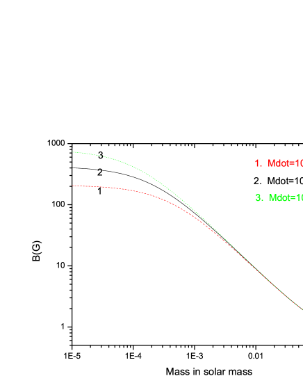
Figure 2: The magnetic field versus accreted mass diagram with various initial field strengths from $B_{o}=10^{6}$ G to $B_{o}=10^{8}$ G as labeled in the figure, where the mass accretion rate is set to be $10^{16}g/cm^{3}$.

ZK06 have argued that as the bottom field is reached, the stellar field lines are redistributed such that, before becoming buried, the surface equatorial field will approach $B_{\rm eq}\longrightarrow B+(R/H)(B_{\rm 0}-B)$ and the polar field will reduce to $B\ll B_{\rm 0}$ yielding $B_{\rm eq}\longrightarrow(R/H)B_{\rm 0}\sim 10B_{\rm 0}$ if we take $H\sim 0.1R$. This means that in an MCV where the field has been significantly affected by accretion, a complicated field structure may be expected.

3.1 Is there evidence for field evolution in MCVs?

In order to assess whether the above solutions could be applicable to the MCVs, we must consider the current ideas on the orbital evolution of CVs and MCVs. CVs are envisioned to evolve to lower orbital periods following first contact (initial Roche lobe overflow after common envelope evolution). The loss of orbital angular momentum is driven either by magnetic braking (MB) by the wind that emanates from the secondary, and/or by gravitational radiation (GR). A typical system that first comes into contact (say with $P_{\rm orb}\sim 8$ hr) will evolve to $P_{\rm orb}\sim 3$ hr driven mainly by MB, at which point the secondary star becomes fully convective. According to the canonical model, MB is drastically reduced at this point, and the star, which is by now out of thermal equilibrium, shrinks within its Roche lobe and mass transfer ceases. . The orbit continues to shrink due to the loss of angular momentum by GR. Mass transfer re-commences when $P_{\rm orb}\sim 2$ hr and the system continues to evolve to shorter periods until the period minimum is reached (see Warner 1995 for a review). Thus, the period range $P_{\rm orb}\sim 2-3$ hr, in which there is an apparent lack of CVs, is referred to as the “CV period gap”. The evidence for a period gap is not as strong in the polars (e.g. Webbink & Wickramasinghe 2002 and references therein).

As a first approximation, one can assume that the secular evolution of a CV is driven by a mean mass transfer rate which is determined by the loss of angular momentum by MB and GR. The mass transfer rate will then depend mainly on the orbital period of the system. However, there are significant uncertainties in formulating a MB law that is applicable to secondary stars of the masses found in CVs. Theoretical studies of the orbital evolution of CVs have shown that mass transfer rates of $\sim 7-12\times 10^{16}$ (g/s) are required at the upper end of the period gap if the observed width of the period gap is to be reproduced (e.g. McDermott & Taam 1989; Hameury, King & Lasota 1991). From the different MB laws that have been considered that satisfy this requirement, we estimate that a CV that first comes into contact with a secondary mass $M_{2}=0.5M_{\odot}$ and a primary mass $M_{1}=0.7M_{\odot}$ ($P_{\rm orb}\sim 5$ hr), $\dot{M}_{\rm MB}\sim\mbox{a few}\times 10^{17}$ g s^-1. On the other hand, $\dot{M}_{\rm GR}\sim\mbox{a few}\times 10^{15}$ g s^-1 for typical systems in the period range $P_{\rm orb}\sim 3-8$ hr. Also relevant to the following discussion is the time scale to cross the $2-3$ hr period gap without mass transfer which can be estimated to be $t_{\rm gap}\sim 4\times 10^{8}$ yr.

The lack of a pronounced period gap in polars has led to the suggestion that these systems evolve much more slowly due to a drastic reduction in the rate of MB. The reduction is attributed to the trapping of the stellar wind in the combined magnetosphere of the two stars in synchronized systems (Li & Wickramasinghe 1998). As a consequence, the secondary remains in near thermal equlibrium during its orbital evolution, and when the field is strong enough to severely curtail MB, no period gap is formed (see Webbink & Wickramasinghe 2002 for results of detailed calculations). As a good first approximation, we can assume that the orbital evolution of most polars is driven by angular momentum loss at a rate that is closer to the GR rate than to the standard MB rate. The mass transfer rate due to GR is typically of a few $\sim 10^{15}$ g s^-1 at $P_{\rm orb}\sim 3$ hr which more than an order of magnitude smaller than the MB rate at the same period.

A disc system such as an IP, will transfer matter at a rate $\sim 10^{17}$ g s^-1, that is well  bf within the regime where an advective solution may be appropriate. Such a system will accrete a mass $\Delta M\mbox{$\,\stackrel{{\scriptstyle\scriptstyle>}}{{\scriptstyle\sim}}\,$}0.2M_{\odot}$ by the time it reaches the period gap, if its initial period of contact is $\mbox{$\,\stackrel{{\scriptstyle\scriptstyle>}}{{\scriptstyle\sim}}\,$}5$ hr and mass transfer is conservative. Thus, a bottom-field state could be reached. On the other hand, a typical polar will accrete at a reduced rate of $10^{15}$ g s^-1 and no field evolution or decrease in polar field strength will be expected, even though it may eventually accumulate a similar amount of mass.

However, it is by no means clear whether mass will accumulate on the white dwarf during the secular evolution of a CV at the mass transfer rates estimated above. The orbital evolution is expected to be punctuated by nova explosions on time scales of $\sim 10^{4}-10^{5}$ yr during which possibly most of the accreted mass will be ejected from the white dwarf (Townsley & Bildsten 2004). If this is the case, the bottom-field state may not be achieved even in systems that accrete via a disc at a high rate.

In cases where significant field restructuring has occurred, we expect to observe MWDs in CVs with enhanced equatorial field strengths relative to what is expected for a centred dipole configuration. This may be reflected in the presence of dominant higher order moments in the observed surface field distributions. Detailed observations of white dwarfs in MCVs have enabled field structures to be determined only for a handful of systems. Although there is evidence for non-dipolar field structures in many polars, and for the presence of dominant multipolar components in some cases (e.g. Beuermann et al. 2007; Reinsch et al. 2005), such large field variations across the stellar surface are clearly not observed. Thus, if accretion-induced field restructuring has occurred in polars, it must be at a very modest level. Unfortunately, we have no knowledge of field structure in disc systems, including the IPs where we may expect the largest re-structuring/decline of the polar field.

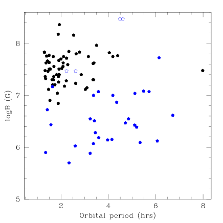
Figure 3: Magnetic field versus orbital period diagram for the polars (filled circles) and IPs (filled triangles). The empty triangles represent IPs which are very close to synchronism. Note that the IP magnetic fields are not directly measured, but simply inferred (values from Norton et al. 2004).

We show in Figure 3 the observed distribution of magnetic field strengths in MCVs as a function of orbital period. If we focus on polars, and assume that they typically evolve from long orbital periods through the period gap as MCVs, there is no evidence for an evolution from high fields to low fields. Indeed, if at all, the evidence appears to be in the opposite direction.

If we look at the entire class of MCVs (IPs and Polars), we note that the ratio of the number of polars to IPs is much higher below the gap as compared to above the gap. This has often been interpreted as evidence in support of the hypothesis that IPs above the period gap may evolve into AM Hers below the period gap. It is indeed the case that the time-scale to cross the period gap is similar to the diffusion time scale $t_{\rm diff}(eq)$ for an accreted mass $\Delta M\sim\Delta M_{\rm crit}\sim 0.2M_{\odot}$ (see section 2.2). This suggests that a submerged equatorial field in a system that has evolved as an IP above the period gap may diffuse outwards during the period gap when accretion ceases. For $\Delta M\ll\Delta M_{\rm crit}$, as a first approximation, we may simply assume that accretion screens the field (Cumming 2005). We may then expect the field to re-emerge to near its original value in the period gap. On the other hand, when $\Delta M\sim\Delta M_{\rm crit}$, the screening approximation will no longer be appropriate, and we may expect the field to re-emerge with a significantly decreased polar field strength. The apparent increase in the ratio of AM Hers to IPs as one crosses the period gap could partly be due to screening above the period gap. However, the dominant effect may be the greater ease with which systems can lock into synchronism below the gap due to the combination of a lower mass transfer rates and a shorter orbital period (Wu & Wickramasnghe 1991).

It is possible that systems that evolve from sufficiently long orbital periods may accrete sufficient mass even in the presence of nova eruptions to reach a bottom-field state. Therefore, this depends on the efficiency with which mass is ejected in a nova explosion which remains uncertain. We predict that if such systems exist, they will form a sub-class of CVs with discs with distinctive homogeneous properties. Their polar field strengths would be expected to be $B_{\rm f}\sim 3\times 10^{3}$ G and they should have strongly non-dipolar magnetic field structures.

Their spin frequency should be a fraction $\psi$ of the Keplerian spin frequency at the magnetospheric radius $R_{\rm M}\sim R$:

$$\nu_{s}=0.03(Hz)\left(\frac{\psi}{0.5}\right)~{}A,\qquad P=33~{}({\rm s})\left(\frac{0.5}{\psi}\right)\left(\frac{1}{A}\right)$$ (17)

where

$$A=\left(\frac{M}{M_{\odot}}\right)^{1/2}\left(\frac{R}{10^{9}{\rm cm}}\right)^{-3/2}$$

Observations of Low Mass X-ray Binaries (LMXBs) have shown that the maximum spin frequency of a neutron star is 619 Hz, which is roughly half the measured maximum kHz QPO frequency 1330 Hz, that is conventionally ascribed to the Keplerian frequency (van der Klis 2000; 2006). By analogy, we may assume $\psi\sim 0.5$ which suggests that systems that reach the bottom-field state should have spin periods of $\sim 30$ s which is close to the fastest spin periods observed in CVs. We show in Figure 4 the relation between accreted mass and spin period for different values of the initial magnetic field $B_{0}$ at a fixed mass accretion rate of $10^{16}$ g s^-1.

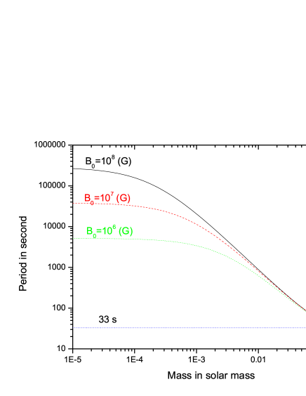
Figure 4: The spin period of WD versus accreted mass diagram with various initial field conditions, where the mass accretion rate is set to be $10^{16}$ g cm^-3.

Magnetic fields are expected to play a role in explaining QPO behaviour in the accreting neutron stars in Low Mass X-ray Binaries (LMXBs). In many respects, the properties of the QPOs observed in the dwarf novae parallel what is seen in neutron stars in the LMXBs (see the review by Warner & Woudt 2008 and references therein) and so it may be tempting to identify the dwarf novae (DN) that exhibit QPO oscillations with MCVs that have reached the bottom-field state.

It should be noted that only $25$% of CVs are magnetic and, if at all, only a small fraction of these systems could have reached the bottom-field state. Thus, one should expect that the vast majority of the DN are likely to be systems that are born with low fields ($\mbox{$\,\stackrel{{\scriptstyle\scriptstyle<}}{{\scriptstyle\sim}}\,$}10^{3}$  G) and a distribution similar to that inferred for the low field isolated magnetic white dwarfs (see next section).

3.2 The field distributions of MCVs and isolated magnetic white dwarfs

As noted in the introduction and illustrated in Figure 1, there are distinct differences in the field distribution of MCVs and of isolated HFMWDs. The peak of the distribution for MCVs occurs at $3\times 10^{7}$ compared to $\sim 10^{7}$ G for the HFMWDs. Generally, compared to the HFMWDs, there is a dearth of low field systems and the very high field systems are not as well represented among the MCVs. The lack of high field systems may be simply related to the extreme reduction that is expected in MB, and hence in the mass transfer rate in such systems which will make them faint and thus much more difficult to detect (e.g. Li, Wu & Wickramasinghe 1994). The apparent lack of low-field MCVs, however, is harder to explain.

In assessing the statistics, we note that there are currently about 40% of polars with no field determinations. It is possible that observations will reveal that most of these systems have magnetic fields between $\sim 2-20$ MG. If we assume that this is the case, and that the fields are distributed as a Gaussian in the logarithm with a mean $\langle\log\rangle B=6.8$ and a standard deviation $\sigma_{\log B}=0.25$, we obtain the results shown in the bottom panel of Figure 5. The distribution of magnetic fields in MCVs and HFMWDs then become similar, and a strong case cannot be made for field decay. On this scenario, it has to be assumed that most systems that are observed as IPs above the period gap will synchronize in the period gap and be seen as polars below the gap thus explaining the observed reduction in the ratio of IPs to polars below the gap.

On the other hand, if observations show that the 40% of polars with no field determinations have fields similar to those measured in the remaining 60% of polars, then the reduction in the ratio of IPs to polars below the gap can be attributed to effects of accretion on the field.

Figure 5: Top panel: the magnetic field distribution of the HFMWDS. Middle panel: the magnetic field distribution of the MCVs. Here the field strength of most IPs has been inferred on the assumption that the white dwarf is in spin equilibrium with an accretion disc. Bottom panel: the magnetic field distribution of the MCVs obtained by assuming that 40% of polars with no field determinations have magnetic fields between $\sim 2-20$ MG (see text).

The magnetic properties of the isolated LFMWDs and their incidence are less well established, due to current limitations of measuring fields $\mbox{$\,\stackrel{{\scriptstyle\scriptstyle<}}{{\scriptstyle\sim}}\,$}10^{3}$ G. Thus, it is possible that either all WDs are magnetic at some level or that most WDs are essentially non magnetic. In any case, the LFMWDs are likely to be associated with the vast majority of the CVs that show no direct evidence for coherent pulsations at the spin period of the white dwarf as would be expected if there were magnetically channelled accretion on to the surface of the white dwarf . Unfortunately, we have no direct evidence of the field strengths of the white dwarfs in such CVs with discs (e.g. in dwarf novae).

4 Summary and conclusions

The anomalously low fields that have been deduced for the neutron stars in the majority of LMXBs ($10^{8}-10^{10}$ G) compared to the magnetic fields in the isolated radio pulsars ($10^{11}-10^{14}$ G) is seen as strong evidence for accretion-induced field decay (e.g. Manchester 2006). In these disc accretors, the competition between the advection of the field from polar to equatorial regions, and the tendency of the field to re-emerge by Ohmic diffusion results in a net reduction of the field at least during phases of accretion. On the other hand, if the LMXBs do evolve into the BMSPs as is generally assumed (but see Hurley et al. 2009; Ferrario & Wickramasinghe 2007), one can also conclude that the field does not re-emerge when accretion ceases, at least not on the time scale of the typical age ($\sim\mbox{a few}10^{9}$ yr) of a BMSP. The latter conclusion would imply that accretion does not simply lead to a screening of the magnetic field which subsequently re-emerges to near its original value, but would yield a change in the current forming regions, and thus to field decay.

We have investigated whether a similar process may be in operation in accreting MWDs in the CVs. In particular, we have asked whether there is evidence for the existence of group of systems that have reached a bottom field among the CVs.

We have argued that the mass transfer rates that determine the secular evolution of CVs is different for systems that evolve as polars or as IPs. Based on our simplified model for the evolution of the field due to advection, and estimates of times scales of Ohmic diffusion, we conclude as follows.

1. In the advection dominated regime, we expect that as matter accretes on to the polar caps, the field lines will be dragged from the polar caps towards the equator. The bottom-field state is reached when $\sim 0.2M_{\odot}$ is accreted and the equatorial field becomes buried below the white dwarf surface. Systems that enter a bottom-field state will have no memory of initial conditions (initial field and spin period) and are expected to form a homogeneous group with $B_{\rm f}\sim 3\times 10^{3}$ G, and $P\sim 30$ s.

2. The advection dominated solution is expected to be applicable only for accretion rates above a critical value $\dot{M}_{\rm crit}\sim 10^{16}g/s$. Below this rate, the field will diffuse outwards faster than it is advected. The polars, with typical secular mass transfer rates of a few times $10^{15}$ g s^-1, are therefore not expected to exhibit significant field restructuring and reduction in polar field strength. This is consistent with the general lack of evidence for field evolution with orbital period in polars.

3. The advection dominated solution is expected to be applicable to the IPs above the period gap, which typically have accretion rates of $\sim 10^{17}$ g s^-1. Systems that first come into contact at $P_{\rm orb}5$ hr will accrete $\Delta M0.2M_{\odot}$ as they reach the upper end of the period gap ($P_{\rm orb}\sim 3$ hr) if mass transfer is conservative. However, when nova eruptions are taken into consideration, the mass that is built up by accretion may be significantly smaller. We may therefore expect only a small proportion of IPs, if any, to reach the bottom-field state.

4. If there are MCVs that have reached the bottom-field state, they are likely to be found among the dwarf novae that exhibit QPOs. They may be expected to have very peculiar field structures dominated by strong equatorial field enhancements. However, this prediction cannot be easily verified, since we have little information on the field structures of white dwarfs in disc accreting systems.

   We conclude by noting that there are two major differences between LMXBs and CVs that make field restructuring and /or decay more likely in the LMXBs. Due to vastly different magnetic moments of the neutron stars (typically lower by a factor $\sim 10^{6}$), there are no magnetically phase locked systems similar to the polars. Thus, while the majority of the CVs that are recognised to be magnetic are the strong field polars, which we have argued are unlikely to exhibit accretion induced field restructuring due to their intrinsically lower mass accretion rates, all the LMXBs (which include both high and low field neutron stars) are disc systems with intrinsically higher mass transfer rates, and are therefore more likely to exhibit field restructuring and /or decay. A second major difference is that thermonuclear runaways similar to nova explosions in CVs are not expected to result in mass loss from neutron stars, because of their deep gravitational potential, so that the critical mass is likely to be achieved more easily during LMXB evolution.

References

- (1) Beuermann K., Euchner F., Reinsch K. et al., 2007, 463, 647
- (2) Butters O.W., Katajainen S., Norton A.J., Lehto H.J., Piirola V., 2009, A&A, in press, arXiv:0901.3516
- (3) Cumming A. 2002, MNRAS, 333, 589 (C02)
- (4) Cumming A. 2003, in proceedings of the conference ”White Dwarfs”, held at Napoli, Italy, Edited by D. de Martino, R. Silvotti, J.-E. Solheim, and R. Kalytis, Kluwer Academic Publishers, NATO Science Series II, Vol. 105, p. 183
- (5) Cumming A. 2004, in “Magnetic Cataclysmic Variables”, ASP Conference Proceedings, San Francisco: Astronomical Society of the Pacific, 2004., 315, 58
- (6) Cumming A. 2005, in “Binary Radio Pulsars”, ASP Conference Series, Eds: F. A. Rasio & I. H. Stairs, San Francisco: Astronomical Society of the Pacific, 328, 311
- (7) Morin, J., et al., 2008, MNRAS, 390, 567
- (8) Ferrario L., Wickramasinghe, D. T., 1993, MNRAS, 265, 605
- (9) Ferrario L., Wickramasinghe D. T. & King, 1993, MNRAS, 260, 149
- (10) Ferrario L., Wickramasinghe D. T., 2007, MNRAS, 375, 1009
- (11) Ghosh P., Lamb F.K., 1979, ApJ, 232, 259; 234, 296
- (12) Hurley J.R., Wickramasinghe, D.T., Ferrario L., Tout C.A., Kiel P., 2009, MNRAS, submitted
- (13) Itoh N., Mitake S., Iyetomi H., Ichimaru S., 1983, ApJ , 273, 774
- (14) Hameury, J. M., King, A. R., Lasota, J.-P., 1991, A&A, 248, 525
- (15) Konar, S., & Choudhury, A. 2004, MNRAS , 348, 661
- (16) Li X. D., & Wang Z.R. 1999, ApJ , 513, 845
- (17) Li J., Wu K., Wickramasinghe D. T. 1994, MNRAS, 270, 769
- (18) Li J., Wickramasinghe D. T., 1998, MNRAS , 300, 718
- (19) Manchester, R.N. 2006, Advances in Space Research 38, 2709
- (20) McDermott P. N., Taam, Ronald E., 1989, ApJ, 342, 1019
- (21) Morin J., Donati J.-F., Forveille T., et al., 2008, MNRAS, 384, 77
- (22) Norton A. J., Wynn G.A., Somerscales R.V., 2004, ApJ, 614, 349
- (23) Patterson J., 1994, PASP , 106, 209
- (24) Payne, D., & Melatos, A. 2004, MNRAS , 351, 569
- (25) Reinsch K., Euchner F., Beuermann K., et al., 2005, in Proceedings of ASP Conference, The Astrophysics of Cataclysmic Variables and Related Objects, Edited by J.M. Hameury and J.P. Lasota, San Francisco, ASP, Vol. 330, p.177,
- (26) Romani R. W., 1990, Nature , 347, 741
- (27) Shapiro S.L., & Teukolsky S.A. 1983, in “Black Holes, White Dwarfs and Neutron Stars”. Wiley, New York
- (28) Schatz H., Bildsten L., Cumming A., Wiescher M., 1999, ApJ , 524, 1014
- (29) Townsley D. M., Bildsten L., 2004, ApJ , 600, 390
- (30) van der Klis, M. 2000, ARA&A, 38, 717
- (31) van der Klis, M. 2006, “A review of rapid X-ray variability in X-ray binaries”, in Compact stellar X-ray sources, eds. W.H.G. Lewin & M. van der Klis, Cambridge University Press, p.39
- (32) Warner B., 1995, Cataclysmic Variable Stars (Cambridge: Cambridge University Press)
- (33) Warner B., Woudt, P. A. 2002, MNRAS, 335, 84
- (34) Warner B., Woudt P. A. 2008, in “Cool discs, hot flows: The varying faces of accreting compact objects”, AIP Conf. Series, Vol. 1054, p 101
- (35) Warner, B., Pretorius M.L. 2008, MNRAS, 383, 1469
- (36) Webbink R. F., Wickramasinghe, D. T., 2002, 335, 1
- (37) Wickramasinghe D. T., Ferrario L., 1988, ApJ, 334, 412
- (38) Wickramasinghe D. T., Ferrario L., 2000, PASP , 112, 873 (WF00)
- (39) Wickramasinghe D.T., Ferrario L. 2009, Astrophysics & Space Science Library, Springer-Verlag: Dordrecht, in press
- (40) Wijnands, R., & van der Klis, M. 1998, Nature, 394, 344 249, 460
- (41) Wood, M. A. et al. 2000, Baltic Astronomy, 9, 210
- (42) Wu K., Wickramasinghe D. T., 1991, MNRAS , 252, 386
- (43) Yakovlev D. G., Urpin V. A., 1980, Soviet Astron, 24, 303
- (44) Zhang, C. M. & Kojima, Y., 2006, MNRAS, 366, 137 (ZK06)