High-field instability of field-induced triplon Bose-Einstein condensate

Abstract

We study properties of magnetic field-induced Bose-Einstein condensate of triplons as a function of temperature and the field within the Hartree-Fock-Bogoliubov approach including the anomalous density. We show that the magnetization is continuous across the transition, in agreement with the experiment. In sufficiently strong fields the condensate becomes unstable due to triplon-triplon repulsion. As a result, the system is characterized by two critical magnetic fields: one producing the condensate and the other destroying it. We show that nonparabolic triplon dispersion arising due to the gapped bare spectrum and the crystal structure has a strong influence on the phase diagram.

Bose-Einstein condensation (BEC), a macroscopic quantum phenomenon, occurs in various systems of bosons, including, in addition to atoms, quasiparticles in systems out of equilibrium such as excitons and polaritons (for example,Snoke07 ). Theory predicts that quantum spin excitations in solids, being Bose-quasiparticles, can at certain conditions build the condensate, and magnetic ordering in various sysems can be understood in terms of the BEC of these excitations.Matsuda ; Tachiki ; Batyev ; Affleck ; Giamarchi99 The first experimental observation Nikuni00 of magnetic field-induced BEC of triplons, that is the spin $S=1$ quasiparticles, in antiferromagnetic TlCuCl₃ produced a diverse research field. Crisan05 ; Stone07 ; Ruegg07 ; Yamada08 ; Amore08 ; Aczel09 ; Paduan09 ; Laflorencie09 ; Demidov08 ; Giamarchi08 In this compound, the triplon branches with $S_{z}=-1,0,1$, are separated from the ground state by a relatively small gap $\Delta$. For this reason, the Zeeman interaction in a modest external magnetic field $H_{\rm ext}$ can close the gap for the $S_{z}=-1$ states. In contrast to atomic gases, where the total particle number is constant, for triplons it is proportional to magnetization $M(T,H_{\rm ext})$ induced by $H_{\rm ext}$. The density of triplons rapidly increases with the field, and they undergo the BEC leading to a magnetic ordering. This field-induced BEC, which occurs at the scale on the order of few K, has been observed in a variety of quantum antiferromagnets.Giamarchi08

The condensate properties crucially depend on interaction of the particles.Huangbook For the atomic BEC at $T=0$ the interatomic repulsion can lead to the condensate instability when the concentration becomes large enough.Rakhimov08 Another general feature clearly seen in the triplon BEC is the dependence of its physics on the bare dispersion of the quasiparticles $\varepsilon_{\bf k}$. The non-parabolic bare dispersion of triplons Misguich04 leads to a non-trivial dependence of the transition temperature $T_{\rm c}$ on the concentration $\rho\sim M(T,H_{\rm ext})$ and, hence, on $H_{\rm ext}$. The bare dispersion, being itself $H_{\rm ext}$-independent, determines the interplay of kinetic and potential energy of a macroscopic system, and, therefore, plays a crucial role in the BEC properties. The effects of the bare dispersion are clearly seen experimentally as the $\rho$-dependence $T_{\rm c}\sim\rho^{\phi(\rho)}$. The exponent ${\phi(\rho)}$ approaches $2/3$ at low concentrations (low $T_{c}$),Yamada08 as predicted for the parabolic $\varepsilon_{\bf k}$, while at $T>2.5$ K, ${\phi(\rho)}$ is close to 0.5.

Here we establish theoretical phase diagram of the field-induced triplon BEC based on the Hartree-Fock-Bogoliubov (HFB) approximation taking into account also a nonparabolic dispersion and determine the fields $H_{\rm ext}^{(1)}$ and $H_{\rm ext}^{(2)}>H_{\rm ext}^{(1)}$, corresponding to the BEC onset and to the instability. A problem in the current theoretical description of the transition at $H_{\rm ext}^{(1)}$ is its predicted discontinuity. We show that this result is an artefact of the conventional Hartree-Fock-Popov (HFP) approximation, neglecting the anomalous density terms. When the anomalous density is taken into account, the theory correctly predicts the continuous transition. For this reason, the HFB method is more appropriate to study the BEC than the HFP one. We find here the stability region of the triplon BEC in the $T-H_{\rm ext}$ plane and prove that its boundaries strongly depend on the dispersion $\varepsilon_{\bf k}$. Results on triplons and on cold atoms can be compared to foster the understanding of the similarities and differences of their BEC.

The triplons form a non-ideal Bose gas Batyev ; Nikuni00 ; Misguich04 with contact repulsive interaction described by the Hamiltonian:

$$\begin{array}[]{l}\hat{H}=\displaystyle\int dV\Big{\{}\psi^{\dagger}({\bf r}){\cal K}\psi({\bf r})+\displaystyle\frac{g}{2}[\psi^{\dagger}({\bf r})\psi({\bf r})]^{2}\Big{\}},\end{array}$$ (1)

where ${\cal K}$ is the kinetic energy operator and $g$ is the coupling constant, and we adopt the units $k_{B}=1$, $\hbar=1$, and $V=1$ for the crystal volume. Below the critical temperature $T_{\rm c}$ the global gauge symmetry becomes broken as realized by the Bogoliubov shift in the field operator: $\psi({\bf r})=v+\widetilde{\psi}({\bf r})$. Here the condensate order parameter $v$ and $\widetilde{\psi}({\bf r})$ define the density of condensed and uncondensed particles, respectively: $\displaystyle{\rho_{0}}=v^{2}$, $\displaystyle{\rho_{1}}=\langle{\widetilde{\psi}}^{\dagger}({\bf r})\widetilde{\psi}({\bf r})\rangle.$ The grand canonical Hamiltonian is: $\hat{H}_{G}=\hat{H}-\mu\rho$, where $\mu$ is the chemical potential and the total density $\rho=\rho_{0}+\rho_{1}$ is uniquely determined by $H_{\rm ext}$. The density $\rho$ is considered as a dimensionless quantity. After the Bogoliubov shift one presents the grand Hamiltonian $\hat{H}_{G}$ in terms of second quantization operators as $\hat{H}_{G}=H_{0}+H_{1}+H_{2}+H_{3}+H_{4}$ with:Andersen04

$$H_{0}=-\mu\displaystyle{\rho_{0}}+\displaystyle\frac{g\rho_{0}^{2}}{2},$$ (2)

$$H_{2}={\displaystyle\sum}_{\bf k}^{\prime}\left[\left(\varepsilon_{\bf k}-\mu+2g\displaystyle{\rho_{0}}\right){a}^{\dagger}_{\bf k}a_{\bf k}+\displaystyle\frac{g\displaystyle{\rho_{0}}}{2}\left(a_{\bf k}a_{\bf-k}+{\rm h.c.}\right)\right],$$

$$H_{4}=\displaystyle\frac{g}{2}{\sum}_{\bf k,p,q}^{\prime}{a}^{\dagger}_{\bf k}{a}^{\dagger}_{\bf p}a_{\bf q}a_{\bf k+p-q},$$

where the prime shows that zero momentum states are excluded. Similarly defined linear ($H_{1}$) and cubic ($H_{3}$) terms having zero mean-field approximation (MFA) expectation values are omitted.

Now we implement the HFB approximation yukalov ; Andersen04 :

$${a}^{\dagger}_{\bf k}{a}^{\dagger}_{\bf p}a_{\bf q}a_{\bf m}\rightarrow 4{a}^{\dagger}_{\bf k}a_{\bf m}\langle{a}^{\dagger}_{\bf p}a_{\bf q}\rangle+a_{\bf q}a_{\bf m}\langle{a}^{\dagger}_{\bf k}{a}^{\dagger}_{\bf p}\rangle+{a}^{\dagger}_{\bf k}{a}^{\dagger}_{\bf p}\langle a_{\bf q}a_{\bf m}\rangle-2\rho_{1}^{2}-\sigma_{1}^{2},$$ (3)

where $\langle{a}^{\dagger}_{\bf k}a_{\bf p}\rangle=\delta_{{\bf k},{\bf p}}n_{\bf k}$, $\langle a_{\bf k}a_{\bf p}\rangle=\delta_{{\bf k},{-\bf p}}\sigma_{\bf k}$, $n_{\bf k}$ and $\sigma_{\bf k}$ are related to the normal $\displaystyle{\rho_{1}}=\displaystyle\sum_{\bf k}n_{\bf k}$ and anomalous $\displaystyle{\sigma_{1}}=\displaystyle\sum_{\bf k}\sigma_{\bf k}$ densities. The grand Hamiltonian in this approximation involves only zero $\widetilde{H}_{0}$ and second order $\widetilde{H}_{2}$ contributions in $a_{\bf k},{a}^{\dagger}_{\bf k}$:

$$\begin{array}[]{l}\widetilde{H}_{0}=-\mu\displaystyle{\rho_{0}}+\displaystyle\frac{g}{2}\left[\rho_{0}^{2}-2\rho_{1}^{2}-\sigma_{1}^{2}\right],\\ \widetilde{H}_{2}={\displaystyle\sum}_{\bf k}^{\prime}\left[\omega_{\bf k}{a}^{\dagger}_{\bf k}a_{\bf k}+\displaystyle\frac{X_{1}}{4}\left(a_{\bf k}a_{\bf-k}+{\rm h.c.}\right)\right],\end{array}$$ (4)

where $\omega_{\bf k}=\varepsilon_{\bf k}-\mu+2g\rho$ and

$$X_{1}=2g(\displaystyle{\rho_{0}}+\displaystyle{\sigma_{1}}).$$ (5)

It follows from (4) that for $T>T_{\rm c}$ the $\widetilde{H}_{2}$ term is diagonal and hence, the triplon density is given by the same formula as in the widely used HFP approximation

$$\rho(T>T_{\rm c})=\displaystyle\sum_{\bf k}\displaystyle\frac{1}{e^{\omega_{\bf k}}/T-1}\equiv\displaystyle\sum_{\bf k}\displaystyle\frac{1}{e^{(\varepsilon_{\bf k}-\mu_{\rm eff})/T}-1},$$ (6)

where $\mu_{\rm eff}=\mu-2g\rho$. In the BEC regime one performs Bogoliubov transformation

$$a_{\bf k}=u_{\bf k}b_{\bf k}+v_{\bf k}{b}^{\dagger}_{\bf-k},\quad{a}^{\dagger}_{\bf k}=u_{\bf k}{b}^{\dagger}_{\bf k}+v_{\bf k}b_{\bf-k},$$ (7)

with $[b_{\bf k},{b}^{\dagger}_{\bf p}]=\delta_{{\bf k},{\bf p}}$, $\langle{b}^{\dagger}_{\bf k}{b}^{\dagger}_{\bf-k}\rangle=\langle b_{\bf k}b_{\bf-k}\rangle=0.$ As a result, the grand Hamiltonian is transformed to the Bogoluibov form:

$$\begin{array}[]{l}H=\widetilde{H}_{0}+\displaystyle\sum_{\bf k}E_{\bf k}{b}^{\dagger}_{\bf k}b_{\bf k}+\displaystyle\frac{1}{2}\displaystyle\sum_{\bf k}(E_{\bf k}-\omega_{\bf k}),\end{array}$$ (8)

where $\langle{b}^{\dagger}_{\bf k}b_{\bf k}\rangle=n_{B}(E_{\bf k},T)=1/[\exp(E_{\bf k}/T)-1]$ with the phonon Goldstone mode dispersion $E_{\bf k}^{2}=\omega_{\bf k}^{2}-X_{1}^{2}/4$. At small momenta, this mode is a collective excitation of the condensate carrying spin $S_{z}=-1$, while at large momenta it becomes the bare triplon mode.

In accordance with Hugenholtz-Pines theorem Dickhoffbook at small $k$ the phonon dispersion is linear: $E_{\bf k}\sim ck+O(k^{2})$, where $c$ can be interpreted as the speed of sound. This is achieved by setting $\omega_{\bf k}-X_{1}/2=\varepsilon_{\bf k}$, that is, by:

$$\mu-g\displaystyle{\rho_{0}}-2g\displaystyle{\rho_{1}}+g\displaystyle{\sigma_{1}}=0.$$ (9)

This choice yields $E_{\bf k}=\sqrt{\varepsilon_{\bf k}(\varepsilon_{\bf k}+X_{1})}$ with $c=\sqrt{X_{1}/2m}$, where $m$ is the triplon effective mass. It can be shown Andersen04 ; Rakhimov08 that $X_{1}$ is related to the normal and anomalous self energies as $\Sigma_{\rm n}=X_{1}/2+\mu$ and $\Sigma_{\rm a}=X_{1}/2$, respectively. The quantity $X_{1}$ plays a special role in our analysis: when $X_{1}>0$, the condensate is stable, otherwise it decays due to triplon-triplon interaction. booknikinu ; Ma71 ; Chung08 Below we find $X_{1}$ in the $T-H_{\rm ext}$ plane and determine the stable BEC region by the condition $X_{1}\geq 0$.

Using the explicit $u_{\bf k}=\sqrt{(\omega_{\bf k}+E_{\bf k})/2E_{\bf k}}$ and $v_{\bf k}=\sqrt{(\omega_{\bf k}-E_{\bf k})/2E_{\bf k}}$, one obtains:

$$\rho_{1}=\displaystyle\sum_{\bf k}\langle{a}^{\dagger}_{\bf k}a_{\bf k}\rangle=\displaystyle\sum_{\bf k}\left(\displaystyle\frac{\omega_{\bf k}W_{\bf k}}{E_{\bf k}}-\displaystyle\frac{1}{2}\right),$$

$$\sigma_{1}=\displaystyle\sum_{\bf k}\langle a_{\bf k}a_{\bf-k}\rangle=2\displaystyle\sum_{\bf k}u_{\bf k}v_{\bf k}W_{\bf k}=-\displaystyle\frac{X_{1}}{2}\displaystyle\sum_{\bf k}\displaystyle\frac{W_{\bf k}}{E_{\bf k}},$$ (10)

where $W_{\bf k}=n_{B}(E_{\bf k},T)+1/2$. Near the transition, $T\rightarrow T_{\rm c}$ the condensate fraction vanishes: $\rho_{0}\rightarrow 0$, and Eq.(5) yields $X_{1}=0$. In the triplon BEC, the critical density $\rho_{c}$ corresponds to $\mu_{\rm eff}=0$, i.e. $\rho_{c}=\mu/2g$. Therefore, at a given chemical potential $\mu=\widetilde{g}\mu_{B}H_{\rm ext}-\Delta$, where $\widetilde{g}$ is the electron Landé-factor, $T_{\rm c}$ is determined by: $\Sigma_{\bf k}n_{B}(\varepsilon_{\bf k},T_{\rm c})={\mu}/{2g}.$

To perform MFA calculations one starts by solving Eqs.(5) and (9) with $\rho_{1}$ and $\sigma_{1}$ given by Eq.(10). In contrast to the BEC of atomic gases, in the triplon problem, the chemical potential is the input parameter, whereas the densities are the output ones. Bearing this in mind, we rewrite Eqs.(5) and (9) as:

$$X_{1}=2\mu+4g(\displaystyle{\sigma_{1}}-\rho_{1}),\qquad\rho_{0}=\displaystyle\frac{X_{1}}{2g}-\sigma_{1}.$$ (11)

Using dimensional regularization at $T=0$, we can find from (10) more explicit expressions for the densities

$$\begin{array}[]{l}\rho_{1}=\rho_{1}(T=0)+\displaystyle\int\displaystyle\frac{d^{3}k}{(2\pi)^{3}}n_{B}(E_{\bf k},T)\displaystyle\frac{\varepsilon_{\bf k}+X_{1}/2}{E_{\bf k}},\\ \sigma_{1}=\sigma_{1}(T=0)-\displaystyle\int\displaystyle\frac{d^{3}k}{(2\pi)^{3}}n_{B}(E_{\bf k},T)\displaystyle\frac{{X_{1}}/{2}}{E_{\bf k}},\end{array}$$ (12)

where $\sigma_{1}(T=0)=3\rho_{1}(T=0)=\sqrt{2}(mX_{1})^{3/2}/4\pi^{2}$, as shown in Ref.[yukalov, ]. By setting in all above formulas $\sigma_{1}=0$, one arrives at the HFP approximation, Nikuni00 ; Misguich04 and particularly

$$X_{1}^{\rm[HFP]}=2\mu-4g\rho_{1},\qquad\rho_{0}=\displaystyle\frac{X_{1}^{\rm[HFP]}}{2g}.$$ (13)

The above Eqs.(11)-(13) can be applied for any realistic $\varepsilon_{\bf k}$. It is instructive to note that for the parabolic dispersion $\varepsilon_{\bf k}={\bf k}^{2}/2m$, the BEC can be fully described by only two parameters $\eta\equiv\mu m^{3}g^{2}$ and $t\equiv T/T_{\rm c}$ with $T_{\rm c}={\widetilde{c}}\left({\mu}/{g}\right)^{2/3}/{m}$, $\widetilde{c}=\pi\left({\sqrt{2}}/{g_{3/2}(1)}\right)^{2/3}=2.0867$, where $g_{3/2}(z)$ is the Bose function.Huangbook The parameter $\eta$ is an analogue of the gas parameter Huangbook of atomic BEC.

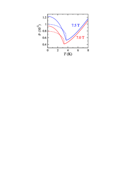
Figure 1: (Color online). Comparison of the HFB (solid) and the HFP (dashed lines) results for the triplon density. The HFB approach shows a continuous behavior, which fully agrees with the experimental data Yamada08 ; Amore08 while the HFP approach leads to the discontinuity. The corresponding $H_{\rm ext}$ are marked near the plots.

Since the MFA (both HFB and HFP) calculations are based on Eqs.(11), (12), a question about the existence of positive solutions for $X_{1}$ arises. To analyze qualitatively the existence of the physical solutions, we consider $T=0$ case. Here, the HFP Eq.(13) is simplified by substitution $Z_{\rm HFP}\equiv X_{1}^{\rm[HFP]}/2\mu$ to $1=Z_{\rm HFP}+{2Z_{\rm HFP}^{3/2}\sqrt{\eta}}/{3\pi^{2}}$ and has physical solutions $Z_{\rm HFP}>0$ for any $\eta>0$. This remains valid for all $t\leq 1$ at any concentration $\rho$. However, in the HFB approximation the situation is different: even at $t\leq 1$, the physical solutions of Eq.(11) can disappear if $\eta$ exceeds a critical value $\eta_{c}$. For example, at $T=0$, Eq. (11) for $Z\equiv X_{1}/2\mu$ simplifies as

$$1=Z-\displaystyle\frac{4Z^{3/2}\sqrt{\eta}}{3\pi^{2}}.$$ (14)

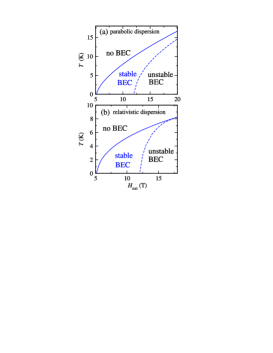
Figure 2: (Color online). Phase diagram for the parabolic (a) and relativistic (b) triplon dispersion in the HFB approximation.

When $\eta$ exceeds $\eta_{c}=\pi^{4}/12$, the rhs in Eq.(14) is less than 1 for any $Z\geq 0$, therefore, it has no positive solutions, and, as a result, $X_{1}$ acquires an imaginary part. Bearing in mind that $\eta=\mu m^{3}g^{2}=(\mu_{B}\widetilde{g}H_{\rm ext}-\Delta)m^{3}g^{2}$, one concludes that even at $T=0$, if the $H_{\rm ext}$ is strong enough the speed of sound $c=\sqrt{Z\mu/m}$ becomes complex and, hence, the BEC is unstable.

To calculate $\rho$ and $X_{1}$ one needs the bare $\varepsilon_{\bf k}$. Misguich and Oshikawa Misguich04 demonstrated that only with the exact $\varepsilon_{\bf k}$ one can explain the overall $\rho_{c}-T_{\rm c}$ - dependence. Here we apply a similar approach, using a simpler, ”relativistic” $\varepsilon_{\bf k}=\sqrt{\Delta^{2}+J^{2}k^{2}/4}-\Delta$, generic for systems with gapped spectrum. This choice leads to $\rho_{c}\sim T_{\rm c}^{2}$ at higher and $\rho_{c}\sim T_{\rm c}^{3/2}$ at lower $T$s, respectively.Sherman03 ; Grether07 Here the effective exchange $J=2\sqrt{\Delta/m}$ is chosen to match the parabolic and the relativistic $\varepsilon_{\bf k}$ at small $k$.

In numerical calculations we used parameters by Yamada et al. Yamada08 for TlCuCl₃: $m=0.0204$ K^-1, (i.e. $m=0.261\times 10^{-25}$ g), unit cell size $0.79$ nm, $\Delta=7.1$ K, $g=313$ K and $\widetilde{g}=2.06$. We neglect a weak renormalization of the model parameters by temperature-dependent many-body effects, which can slightly shift the stability region boundary, since we consider the regime of low $T$ and $\rho$. This assumption yields a perfect agreement of theory and experiment Misguich04 in a similar range of $T$ and $\rho$. We begin with the comparison of the HFB and HFP approaches for the density $\rho$ in a constant $H_{\rm ext}$. Fig.1 shows a continuous plot of $\rho(T,H_{\rm ext})$ obtained with the HFB approach,Sirker04 in full agreement with the experiment Yamada08 ; Amore08 and in contrast to the HFP approximation. In Fig.2 we present the phase diagram obtained in the HFB for the parabolic and the relativistic $\varepsilon_{\bf k}$. Solid curves in these figures present $T_{\rm c}$ vs $H_{\rm ext}$ obtained from $\Sigma_{\bf k}n_{B}(\varepsilon_{\bf k},T_{\rm c})={\mu}/{2g}.$ The dashed lines present the BEC stability boundary: there is no $X_{1}>0$ solutions to the gap equations in the regions below these lines. Therefore, the HFB approach predicts the existence of a stable (the region between solid and dashed lines) and unstable BEC zones (the region below the dashed line). As expected, at low $T$ and small $H_{\rm ext}$ the stability region in Figs. 2(a) and 2(b) is the same for both $\varepsilon_{\bf k}$. In general, the relativistic dispersion leads to a narrower stability zone than the parabolic one. Note that magnetization measurements on TlCuCl₃ have been done for $H_{\rm ext}$ between 5.1 and 9 T.Yamada08 ; Amore08 It would be interesting to experimentally study its behavior at higher $H_{\rm ext}$ to explore the instability region.Tanaka01 A direct access to the dispersion and damping of the phonon-like mode in TlCuCl₃ can be achieved in the inelastic neutron scattering measurements.Ruegg

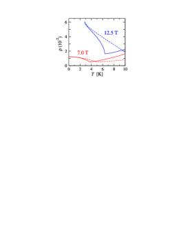
Figure 3: (Color online). Triplon density as a function of $T$ for relativistic (solid) and parabolic (dashed lines) dispersion in the HFB approximation for $H_{\rm ext}$ marked near the plots. The plot for $H=12.5$ T (upper curves) shows two anomalies, one of them caused by the instability.

Density $\rho$ as a function of temperature is presented in Fig.3 for two $H_{\rm ext}$. At relatively weak fields, e.g. $H_{\rm ext}=7.0$ T the magnetization exhibits only one anomaly at $T=T_{\rm c}$ while at stronger one $H_{\rm ext}=12.5$ T, two anomalies are present. The minimum at the solid line at 6.2 K is the onset of the BEC, while the anomaly at $T$ slightly less than 3 K is due to the condensate decay. Similar physical behavior can be seen in Fig.4, which shows the BEC fraction $\rho_{0}/\rho\times 100\%$. This fraction is rather large ($\sim 95\%$ for $H_{\rm ext}=7.5$ T at $T=0$) and rapidly decreases with increasing the temperature. In both Figs.3 and 4 the curves for $H_{\rm ext}=12.5$ T start at $T\approx 3$ K since the BEC is unstable below this $T$. However, Fig.4 shows that even close to this point the condensate fraction is approximately $70\%$, and, therefore, in the instability zone the condensate can exist for a short time Schilling09 determined by the imaginary part of the self energy $X_{1}$. This regime will be considered in an extended paper.

In summary, we have theoretically established the phase diagram of the field-induced triplon BEC in quantum antiferromagnets in the $T-H_{\rm ext}$ plane for a model relevant for the TlCuCl₃ compound. Our approach is based on the HFB approximation taking into account the anomalous density in the condensate phase. We have shown that (i) at the BEC transition the magnetization remains continuous demonstrating a minimum, in agreement with the experiment, (ii) in high magnetic fields the condensate becomes unstable due to the triplon-triplon repulsion, resulting in interaction of quasiparticles, and found the stability boundaries. The non-parabolic dispersion of triplons determined by the crystal structure has the crucial effect on the phase diagram by changing the boundaries $H_{\rm ext}^{(1)}$ and $H_{\rm ext}^{(2)}$ and making the stability region smaller.

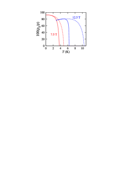
Figure 4: (Color online). Condensate density fraction for relativistic (solid line) and parabolic (dashed line) $\varepsilon_{\bf k}$ in the HFB approximation for $H_{\rm ext}$ marked near the plots.

We acknowledge support of the Volkswagen Foundation (AR) and the University of the Basque Country UPV-EHU Grant GIU07/40 (EYS). AR acknowledges support from Korea Science and Engineering Foundation for visiting fellowship to Yonsei University. We are grateful to H. Kleinert, A. Pelster, and O. Tchernyshyov for valuable discussions.

References

- (1)
- (2) R. Balili et al., Science 316, 1007 (2007), C. W. Lai et al., Nature 417, 47 (2002), J. Keeling, Phys. Rev. B 74, 155325 (2006)
- (3) T. Matsubara and H. Matsuda, Prog. Theor. Phys. 16, 569 (1956); H. Matsuda and T. Tsuneto, ibid 46, 411 (1970);
- (4) M. Tachiki and T. Yamada, J. Phys. Soc. Jpn. 28, 1413 (1970)
- (5) E.G. Batyev and S.L. Braginskii, JETP 60, 781 (1984); E.G. Batyev, ibid 62, 173 (1985)
- (6) I. Affleck, Phys.Rev B 43, 3215 (1991)
- (7) T. Giamarchi and A. M. Tsvelik, Phys. Rev. B 59, 11398 (1999)
- (8) T. Nikuni et al., Phys. Rev. Lett. 84, 5868 (2000)
- (9) M. Crisan et al., Phys. Rev. B 72, 184414 (2005)
- (10) M. B. Stone et al., New J. Phys. 9, 31 (2007)
- (11) Ch. C. Rüegg et al., Phys. Rev. Lett. 98, 017202 (2007)
- (12) F. Yamada et al., J. Phys. Soc. Jpn. 77 013701 (2008)
- (13) R. Dell’Amore, A. Schilling, and K. Krämer Phys. Rev. B 79 014438 (2009); R. Dell’Amore, A. Schilling, and K. Krämer, Phys. Rev. B 78 224403 (2008)
- (14) A. A. Aczel et al., Phys. Rev. B 79, 100409(R) (2009)
- (15) A. Paduan-Filho et al., Phys. Rev. Lett. 102, 077204 (2009)
- (16) N. Laflorencie and F. Mila, Phys. Rev. Lett. 102, 060602 (2009)
- (17) For the BEC in magnetic systems under external pumping: V. E. Demidov et al., Phys. Rev. Lett. 100, 047205 (2008), for theory: Yu. D. Kalafati and V. L. Safonov, JETP Lett. 50, 149 (1989); I. S. Tupitsyn, P. C. Stamp, and A. L. Burin, Phys. Rev. Lett. 100, 257202 (2008); A. I. Bugrij and V. M. Loktev, Low Temp. Phys. 33, 37 (2007).
- (18) T. Giamarchi, C. Rüegg, and O. Tchernyshyov, Nature Physics 4, 198 (2008)
- (19) Kerson Huang, Statistical Mechanics Wiley (1987)
- (20) A. Rakhimov et al., Phys. Rev. A 77, 033626 (2008)
- (21) G. Misguich and M. Oshikawa, J. Phys. Soc. Jpn. 73, 3429 (2004)
- (22) J. O. Andersen, Rev. Mod. Phys. 76, 599 (2004)
- (23) V. I. Yukalov and H. Kleinert, Phys. Rev. A73, 063612, (2006); V.I. Yukalov, Ann. Phys. 323 461 (2008)
- (24) W. H. Dickhoff and D. Van Neck, Many-Body Theory Exposed World Scientific (2005)
- (25) A. Griffin, T. Nikuni and E. Zaremba, Bose-Condensed Gases at Finite Temperatures Cambridge University Press (2009)
- (26) S.-K. Ma, H. Gould, and V. K. Wong, Phys. Rev. A 3, 1453 (1971)
- (27) M.-C. Chung and A. B. Bhattacherjee, New Journ. of Phys. 11, 123012 (2009)
- (28) E. Ya. Sherman et al., Phys. Rev. Lett. 91, 057201 (2003)
- (29) Theory of the BEC in the ideal relativistic Bose gas was developed in M. Grether, M. de Llano, and George A. Baker, Jr., Phys. Rev. Lett. 99, 200406 (2007)
- (30) The continuity can be achieved in the HFP approach with a strong Dzyaloshinskii-Moriya interaction: J. Sirker, A. Weiße, O.P. Sushkov, Europhys. Lett. 68, 275 (2004)
- (31) Neutron scattering experiments by H. Tanaka et al., J. Phys. Soc. Jpn. 70, 939 (2001) explored up to 12 T at K, lower than calculated . To observe unambiguously the effects of instability, experiment has to be performed deeply in the instability region.
- (32) Ch. Rüegg et al., Nature 423, 62 (2003)
- (33) For other aspects of the BEC lifetime see A. Schilling, arXiv:0908.3033v1